A goodness-of-fit test for bivariate extreme-value copulas - arXiv

arX

iv:1

102.

2078

v1 [

mat

h.ST

] 1

0 Fe

b 20

11

Bernoulli 17(1), 2011, 253–275DOI: 10.3150/10-BEJ279

A goodness-of-fit test for bivariate

extreme-value copulas

CHRISTIAN GENEST1, IVAN KOJADINOVIC2, JOHANNANESLEHOVA3 and JUN YAN4

1Departement de mathematiques et de statistique, Universite Laval, 1045, avenue de la Medecine,Quebec, Canada G1V 0A6. E-mail: [email protected] de mathematiques et applications, UMR CNRS 5142, Universite de Pau et des Paysde l’Adour, Boıte postale 1155, 64013 Pau cedex, France. E-mail: [email protected] of Mathematics and Statistics, McGill University, 805, rue Sherbrooke Ouest,Montreal (Quebec), Canada H3A 2K6. E-mail: [email protected] of Statistics, University of Connecticut, 215 Glenbrook Road, Storrs, CT 06269,USA. E-mail: [email protected]

It is often reasonable to assume that the dependence structure of a bivariate continuous dis-tribution belongs to the class of extreme-value copulas. The latter are characterized by theirPickands dependence function. In this paper, a procedure is proposed for testing whether thisfunction belongs to a given parametric family. The test is based on a Cramer–von Mises statisticmeasuring the distance between an estimate of the parametric Pickands dependence functionand either one of two nonparametric estimators thereof studied by Genest and Segers [Ann.Statist. 37 (2009) 2990–3022]. As the limiting distribution of the test statistic depends on un-known parameters, it must be estimated via a parametric bootstrap procedure, the validity ofwhich is established. Monte Carlo simulations are used to assess the power of the test and anextension to dependence structures that are left-tail decreasing in both variables is considered.

Keywords: extreme-value copula; goodness of fit; parametric bootstrap; Pickands dependencefunction; rank-based inference

1. Introduction

Let X and Y be continuous random variables with cumulative distribution functions Fand G, respectively. Following Sklar [36], the joint behavior of the pair (X,Y ) can becharacterized at every (x, y) ∈R2 by the relation

H(x, y) = Pr(X ≤ x,Y ≤ y) =C{F (x),G(y)} (1)

through a unique copula C that captures the dependence between X and Y .

This is an electronic reprint of the original article published by the ISI/BS in Bernoulli,2011, Vol. 17, No. 1, 253–275. This reprint differs from the original in pagination andtypographic detail.

1350-7265 c© 2011 ISI/BS

254 Genest, Kojadinovic, Neslehova and Yan

When H is known, its marginal distributions can easily be retrieved from it. The copulacan also be readily identified as it is simply the joint distribution of the pair (U,V ) =(F (X),G(Y )). In practice, however, H is often unknown, and the relation between Xand Y must be modeled from data.A copula model for H assumes that equation (1) holds for some F , G and C from

specific parametric classes. This approach was used, for example, by Frees and Valdez[11] and Klugman and Parsa [25] to analyze data from the Insurance Services Office,Inc. on the indemnity payment (X) and allocated loss adjustment expense (Y ) for 1500general liability claims randomly chosen from late settlement lags. Based on their workand subsequent analysis by other authors, it is reasonable to assume that for these data,F is inverse paralogistic, G is Pareto and C is a Gumbel–Hougaard extreme-value copula.Extreme-value copulas characterize the limiting dependence structure of suitably nor-

malized componentwise maxima. They are of special interest in insurance [7], finance[6, 29] and hydrology [34], where the occurrence of joint extremes is a risk managementconcern.Pickands [31] showed that if C is a bivariate extreme-value copula, then

C(u, v) = exp

[

log(uv)A

{

log(v)

log(uv)

}]

(2)

for all u, v ∈ (0,1) and a mapping A : [0,1]→ [1/2,1], referred to as the Pickands depen-dence function, which is convex and such that max(t,1− t) ≤A(t) ≤ 1 for all t ∈ [0,1].For instance, an extreme-value copula is said to belong to the Gumbel–Hougaard familyif there exists θ ∈ [1,∞) such that for all t ∈ [0,1], we have

A(t) = {tθ + (1− t)θ}1/θ. (3)

A test that a copula C is of the form (2) was developed by Ghoudi et al. [20]; it wasrecently refined by Ben Ghorbal et al. [1]. Under the assumption that C is an extreme-value copula, it may be of interest to check whether its Pickands dependence function Abelongs to a specific parametric class, say A= {Aθ : θ ∈ O}, where O is an open subsetof Rp for some integer p.The purpose of this paper is to examine how the hypothesis H0 :A ∈ A can be tested

with a random sample (X1, Y1), . . . , (Xn, Yn) from H . As for all goodness-of-fit testsreviewed by Berg [2] and Genest et al. [18], the proposed procedure is based on pseudo-observations (U1, V1), . . . , (Un, Vn) from copula C, defined, for i ∈ {1, . . . , n}, by

Ui = Fn(Xi), Vi =Gn(Yi), (4)

where Fn and Gn are rescaled empirical counterparts of F and G, respectively, given by

Fn(x) =1

n+ 1

n∑

i=1

1(Xi ≤ x), Gn(y) =1

n+ 1

n∑

i=1

1(Yi ≤ y)

Goodness-of-fit testing for extreme-value copulas 255

for all x, y ∈ R. This approach is justified because, as copulas themselves, the pairs(U1, V1), . . . , (Un, Vn) of normalized ranks are invariant under strictly increasing transfor-mations of X and Y . As shown by Kim et al. [24], it also leads to efficient and robustestimators.The proposed test is described in Section 2 and its asymptotic null distribution is given

in Section 3, where a parametric bootstrap is proposed for the calculation of P -values. InSection 4, the distributional result is extended to alternatives that are left-tail decreasingin both variables. This is instrumental in studying the consistency and power of the test,which are considered in Sections 5 and 6, respectively. The paper concludes with anillustrative example. Technical proofs are grouped in a series of appendices.All procedures discussed herein are implemented in the R package copula [38] available

via the Comprehensive R Archive Network at http://cran.r-project.org.

2. Proposed goodness-of-fit test

Let (X1, Y1), . . . , (Xn, Yn) be a random sample from some unknown continuous bivariatedistribution H whose underlying copula is of the form (2) with Pickands dependencefunction A. In order to test the hypothesis

H0 :A ∈A= {Aθ : θ ∈O},

a natural way to proceed is to compare a nonparametric estimator An ofA to a parametricestimator Aθn . Several measures of distance can be used for this purpose, but the Cramer–von Mises statistic

Sn =

∫ 1

0

n|An(t)−Aθn(t)|2 dt (5)

generally leads to more powerful tests than, say, the Kolmogorov–Smirnov statistic [18].The choices of Aθn and An are discussed next.

2.1. Parametric estimation of A

Under H0, Aθ may be estimated by Aθn using a consistent estimate θn of θ. Such anestimate can be derived from the pairs (U1, V1), . . . , (Un, Vn) via the maximum pseudo-likelihood method considered by Genest et al. [14] and Shih and Louis [35].To illustrate this approach in a concrete case, let Aθ be the generator of the Gumbel–

Hougaard copula defined in (3). For all u, v ∈ (0,1), write

Cθ(u, v) = exp

[

log(uv)Aθ

{

log(v)

log(uv)

}]

= exp[−{| log(u)|θ + | log(v)|θ}1/θ].

256 Genest, Kojadinovic, Neslehova and Yan

As Aθ is twice differentiable on (0,1), the copula Cθ has a density given by cθ(u, v) =∂2Cθ(u, v)/∂u∂v everywhere on (0,1)2. The maximum pseudo-likelihood estimator θn isthen the value θ ∈O = (1,∞) at which the function

ℓ(θ) =n∑

i=1

log{cθ(Ui, Vi)}

reaches its global maximum. An advantage of this method is that it can be used evenwhen the parameter space O is multidimensional.When θ is real-valued, a simpler technique which also yields a consistent estimator is

based on the inversion of Kendall’s tau. As shown by Ghoudi et al. [20], the relation

τ(C) =−1 + 4

∫∫ 1

0

C(u, v) dC(u, v) =

∫ 1

0

t(1− t)

A(t)dA′(t)

is valid for any extreme-value copula C. When A ∈ A, τ is a function of θ and a rank-based moment estimate of the latter is obtained by solving the equation τn = τ(θ) forθ, where τn is the sample value of Kendall’s tau. In the Gumbel–Hougaard model, forinstance, we find τ(θ) = 1− 1/θ and hence θn =max{1,1/(1− τn)}.When O ⊂ R, we can also obtain consistent, rank-based estimates of θ by exploiting

its one-to-one relationship with other nonparametric measures of dependence such asSpearman’s rho, that is,

ρ(C) =−3 + 12

∫∫ 1

0

uvdC(u, v) =−1 +

∫ 1

0

1

{A(t)}2 dt.

2.2. Nonparametric estimation of A

Nonparametric estimators of A are proposed by Genest and Segers [19]. For i ∈ {1, . . . , n},set ξi(0) =− log(Ui), ξi(1) =− log(Vi) and

ξi(t) =min

{− log(Ui)

1− t,− log(Vi)

t

}

for all t ∈ (0,1), where Ui and Vi are as in equation (4). Also, let

APn(t) = 1

/

{

1

n

n∑

i=1

ξi(t)

}

, ACFGn (t) = exp

[

−γ − 1

n

n∑

i=1

log{ξi(t)}]

,

where γ =−∫∞

0 log(x)e−x dx≈ 0.577 is Euler’s constant.The functions AP

n and ACFGn are rank-based versions of the estimators of A introduced

by Pickands [31] and Caperaa et al. [4], respectively. As noted by Genest and Segers [19],these estimators can be altered to meet the end-point conditions AP

n(0) =ACFGn (0) = 1

and APn(1) =ACFG

n (1) = 1. However, this makes no difference asymptotically.

Goodness-of-fit testing for extreme-value copulas 257

Both APn and ACFG

n can be expressed as functionals of the empirical copula, which maybe defined for all u, v ∈ [0,1] by

Cn(u, v) =1

n

n∑

i=1

1(Ui ≤ u,Vi ≤ v).

To be specific, the following relations hold for all t ∈ [0,1]:

APn(t) = 1

/

∫ 1

0

Cn(x1−t, xt)

dx

x,

ACFGn (t) = exp

{

−γ +

∫ 1

0

{Cn(x1−t, xt)− 1(x > e−1)} dx

x log(x)

}

.

It was shown by Ruschendorf [33] that under weak regularity conditions, the process√n(Cn−C) converges in law to a Gaussian limit C, that is,

√n(Cn−C) C as n→∞.

We may thus expect APn and ACFG

n to be consistent and asymptotically Gaussian. Thisis shown by Genest and Segers [19], provided that A is twice continuously differentiable.Their Theorem 3.2 states that

APn =

√n(AP

n −A) AP, A

CFGn =

√n(ACFG

n −A) ACFG

as n→∞ in C[0,1], where, for all t ∈ [0,1],

AP(t) = −A2(t)

∫ 1

0

C(x1−t, xt)dx

x,

ACFG(t) = A(t)

∫ 1

0

C(x1−t, xt)dx

x log(x).

Remark. Observe that, in principle, the statistics SPn and SCFG

n could be extendedto arbitrary dimension d≥ 3 because d-variate extreme-value copulas are characterizedby (d− 1)-place Pickands dependence functions [10]. At present, however, multivariateanalogs of the rank-based estimators AP

n and ACFGn are unavailable. To see how the

estimation can proceed in the d-variate case when the marginal distributions are known,refer to [39] or [21].

3. Asymptotic null distribution of the test statistic

The asymptotic distribution of the goodness-of-fit statistic Sn depends on the joint be-havior of Θn =

√n(θn − θ) and either AP

n or ACFGn under H0. Suppose that the class

A= {Aθ : θ ∈O} satisfies the following conditions:

(A) the parameter space O is an open subset of Rp;(B) for every θ ∈O, Aθ is twice continuously differentiable on (0,1);

258 Genest, Kojadinovic, Neslehova and Yan

(C) the gradient Aθ(t) of Aθ(t) with respect to θ satisfies

limǫ↓0

sup‖θ∗−θ‖<ǫ

supt∈[0,1]

‖Aθ∗(t)− Aθ(t)‖→ 0, (6)

where ‖ · ‖ denotes the ℓ2-norm.

As is proved in Appendix A, the process An,θn =√n(An−Aθn) is then asymptotically

Gaussian, both when An =APn and An =ACFG

n .

Proposition 1. Assume H0 holds, that is, C is an extreme-value copula with Pickandsdependence function A = Aθ0 for some θ0 ∈ O. Further, assume that A = {Aθ : θ ∈ O}meets conditions (A)–(C).

(a) If (APn ,Θn) converges to a Gaussian limit (AP,Θ), then An,θn AP − A⊤

θ0Θ as

n→∞ in C[0,1].(b) If (ACFG

n ,Θn) converges to a Gaussian limit (ACFG,Θ), then An,θn ACFG −A⊤

θ0Θ as n→∞ in C[0,1].

The weak convergence of the statistic Sn defined in (5) follows immediately fromProposition 1 and the continuous mapping theorem (see, e.g., [37], Theorem 1.3.6). Asthe limit depends on the unknown parameter value θ0, we must resort to resamplingtechniques to carry out the test. The following parametric bootstrap procedure can beused to this end. Its validity depends on regularity conditions adapted from [17]. Theseconditions, listed in Appendix B, can be verified for many families of extreme-valuecopulas.Parametric bootstrap procedure

(1) Compute An from the pairs (U1, V1), . . . , (Un, Vn) of normalized ranks and estimateθ using a rank-based estimator, as discussed in Section 2.

(2) Compute the test statistic Sn defined in (5).(3) For some large integer N , repeat the following steps for every k ∈ {1, . . . ,N}:

(3.1) generate a random sample (X1k, Y1k), . . . , (Xnk, Ynk) from copula Cθn anddeduce the associated pairs (U1k, V1k), . . . , (Unk, Vnk) of normalized ranks;

(3.2) let Ank and θnk stand for the versions of An and θn derived from the pairs(U1k, V1k), . . . , (Unk, Vnk);

(3.3) compute

Snk =

∫ 1

0

n|Ank(t)−Aθnk(t)|2 dt.

(4) An approximate P -value for the test is given by N−1∑N

k=1 1(Snk ≥ Sn).

4. Extension to left-tail decreasing copulas

The statistic Sn can be used to build goodness-of-fit tests for the more general hypothesis

H∗0 :C ∈ C = {Cθ : θ ∈O},

Goodness-of-fit testing for extreme-value copulas 259

where C is a parametric family of copulas that are left-tail decreasing (LTD) in botharguments. From [30], Exercise 5.35, a copula C is LTD in this sense if and only if, forall 0< u≤ u′ ≤ 1 and 0< v ≤ v′ ≤ 1,

C(u, v)

uv≥ C(u′, v′)

u′v′. (7)

This condition is satisfied for extreme-value copulas, which Garralda-Guillem [13] showedto be stochastically increasing in both variables.The following result, proved in Appendix C, implies that when C is an LTD copula,

APn and ACFG

n are consistent, asymptotically Gaussian estimators of APC and ACFG

C ,respectively, where, for all t ∈ [0,1],

APC(t) = 1

/

∫ 1

0

C(x1−t, xt)dx

x

and

ACFGC (t) = exp

[

−γ +

∫ 1

0

{C(x1−t, xt)− 1(x > e−1)} dx

x log(x)

]

.

Proposition 2. Suppose that the copula C has a continuous density and satisfies condi-tion (7). Then

√n(AP

n −APC) AP

C and√n(ACFG

n −ACFGC ) ACFG

C as n→∞ in C[0,1],where, for all t ∈ [0,1],

APC(t) = −{AP

C(t)}2∫ 1

0

C(x1−t, xt)dx

x,

ACFGC (t) = ACFG

C (t)

∫ 1

0

C(x1−t, xt)dx

x log(x).

Incidentally, the mappings APC and ACFG

C are well defined for any copula C, whetheror not it is LTD. They reduce to the Pickands dependence function A when C is ofthe form (2). Otherwise, they typically differ from one another, but retain some of theproperties of Pickands dependence functions. These facts are summarized in the followingproposition, the proof of which is left to the reader.

Proposition 3. Let C be a copula and let AC denote either APC or ACFG

C . Also, let Wand M denote the lower and upper Frechet–Hoeffding bounds, respectively. The followingstatements then hold:

(a) AW (t)≥AC(t)≥AM (t) =max(t,1− t) for all t ∈ [0,1];(b) if C(u, v)≥ uv for all u, v ∈ [0,1], then AC(t)≤ 1 for all t ∈ [0,1];(c) if C(u, v) =C(v, u) for all u, v ∈ [0,1], then AC(t) =AC(1− t) for all t ∈ [0,1];(d) if C is an extreme-value copula with Pickands dependence function A, then AC =

A.

260 Genest, Kojadinovic, Neslehova and Yan

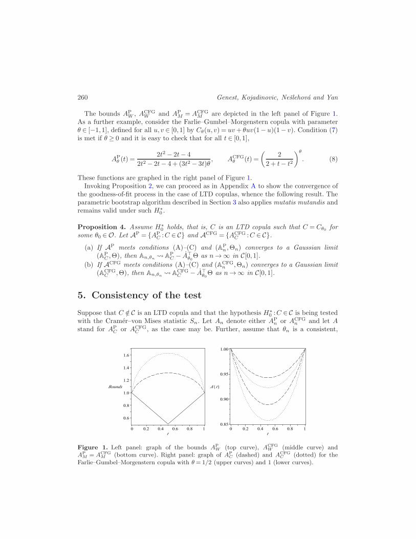
The bounds APW , ACFG

W and APM = ACFG

M are depicted in the left panel of Figure 1.As a further example, consider the Farlie–Gumbel–Morgenstern copula with parameterθ ∈ [−1,1], defined for all u, v ∈ [0,1] by Cθ(u, v) = uv+ θuv(1− u)(1− v). Condition (7)is met if θ ≥ 0 and it is easy to check that for all t ∈ [0,1],

APθ (t) =

2t2 − 2t− 4

2t2 − 2t− 4+ (3t2 − 3t)θ, ACFG

θ (t) =

(

2

2 + t− t2

)θ

. (8)

These functions are graphed in the right panel of Figure 1.Invoking Proposition 2, we can proceed as in Appendix A to show the convergence of

the goodness-of-fit process in the case of LTD copulas, whence the following result. Theparametric bootstrap algorithm described in Section 3 also applies mutatis mutandis andremains valid under such H∗

0 .

Proposition 4. Assume H∗0 holds, that is, C is an LTD copula such that C = Cθ0 for

some θ0 ∈O. Let AP = {APC :C ∈ C} and ACFG = {ACFG

C :C ∈ C}.(a) If AP meets conditions (A)–(C) and (AP

n ,Θn) converges to a Gaussian limit(AP

C ,Θ), then An,θn APC − A⊤

θ0Θ as n→∞ in C[0,1].

(b) If ACFG meets conditions (A)–(C) and (ACFGn ,Θn) converges to a Gaussian limit

(ACFGC ,Θ), then An,θn ACFG

C − A⊤θ0Θ as n→∞ in C[0,1].

5. Consistency of the test

Suppose that C /∈ C is an LTD copula and that the hypothesis H∗0 :C ∈ C is being tested

with the Cramer–von Mises statistic Sn. Let An denote either APn or ACFG

n and let Astand for AP

C or ACFGC , as the case may be. Further, assume that θn is a consistent,

Figure 1. Left panel: graph of the bounds AP

W (top curve), ACFG

W (middle curve) andAP

M = ACFG

M (bottom curve). Right panel: graph of AP

C (dashed) and ACFG

C (dotted) for theFarlie–Gumbel–Morgenstern copula with θ = 1/2 (upper curves) and 1 (lower curves).

Goodness-of-fit testing for extreme-value copulas 261

rank-based estimator of some θ∗ ∈O. The test based on Sn is then consistent, providedthat A 6=Aθ∗ .To see this, decompose the process An,θn as

√n(An −Aθn) =

√n(An −A)−√

n(Aθn −Aθ∗) +√n(A−Aθ∗). (9)

Assume conditions (A)–(C) hold for A = AP or ACFG and that as n→∞, (√n(An −

A),√n(θn − θ∗)) (A,Θ∗) to a Gaussian limit, where A stands for either AP or ACFG.

We can then proceed exactly as in Appendix A to see that as n→∞,√n(An − A)−√

n(Aθn − Aθ∗) A − A⊤θ∗Θ∗. If A 6= Aθ∗ , then supt∈[0,1]

√n|A(t) − Aθ∗(t)| → ∞ and

hence, for every ǫ > 0,

limn→∞

Pr(Sn > ǫ) = 1.

In particular, the test based on Sn is consistent whenever C is an extreme-value copulaand the hypothesized family C also consists of extreme-value copulas. However, consis-tency may fail otherwise, for it may happen that A=Aθ∗ , even if H∗

0 is false.To illustrate this point, consider the functions AP

θ and ACFGθ given in (8). As the latter

are convex, they can be used to generate new families of extreme-value copulas, whichmay be called the FGM–P and FGM–CFG families.Now, suppose that C is the Farlie–Gumbel–Morgenstern copula with parameter θ > 0

and that the statistic Sn is used to test H0 :A ∈A when:

(a) A is the Gumbel–Hougaard family of copulas;(b) A is the FGM–CFG family of extreme-value copulas.

In case (a), the tests based on APn and ACFG

n would be consistent because APθ and ACFG

θ

both differ from the Pickands dependence function of the Gumbel–Hougaard given in (3).In case (b), the test based on AP

n would also be consistent because APθ 6=ACFG

θ∗ . The testbased on ACFG

n may fail to be consistent, however, given that ACFGθ coincides with the

Pickands dependence function of the FGM–CFG family. Consistency of the test wouldthen depend on the behavior of θn.Suppose, for instance, that θ is estimated by inversion of Kendall’s tau. As n→∞,

θn would approach 2θ/9, which is the population value of this dependence measure forthe FGM copula. For the FGM–CFG family, however, Kendall’s tau is 7θ/10 + θ2/30,which coincides with 2θ/9 only when θ = 0, that is, at independence where the differ-ence between the two models is immaterial. Therefore, the test based on ACFG

n wouldbe consistent in this case, provided that θ is estimated by inversion of Kendall’s tau.A similar conclusion would be reached for inversion of Spearman’s rho and maximumpseudo-likelihood estimation.

6. Power study

Equation (9) and the accompanying discussion suggest that just as for consistency, thepower of the test based on Sn depends on how different A = AP

C or ACFGC is from its

262 Genest, Kojadinovic, Neslehova and Yan

Figure 2. Pickands dependence functions of the Gumbel–Hougaard, Galambos, Husler–Reissand t-EV copulas when τ = 0.25, τ = 0.50 and τ = 0.75.

parametric estimate Aθ∗ under H0. This issue is investigated graphically in Section 6.1and via simulations in Sections 6.2 and 6.3.

6.1. General considerations

Consider the following three sets of LTD copula families.

Group I: Symmetric extreme-value copulas : the Gumbel–Hougaard (GH), Galambos(GA), Husler–Reiss (HR) and Student extreme-value (t-EV) copula with four degreesof freedom.

Group II: Symmetric non-extreme-value copulas : the Clayton (C), Frank (F), Normal(N) and Plackett (P).

Group III: Asymmetric extreme-value copulas : asymmetric versions of the Gumbel–Hougaard (a-GH), Galambos (a-GA), Husler–Reiss (a-HR), and Student extreme-value(a-t-EV) copula with four degrees of freedom.

Figure 2 shows the Pickands dependence functions of the copulas in Group I whenτ = 0.25, 0.50, 0.75. Although the curves are not identical, they are very similar. Whenthe statistic Sn is used to distinguish between these models, therefore, the test will beconsistent, but can be expected to have little power, even in moderate sample sizes.In Figure 3, the functions AP

C and ACFGC are plotted for the copulas in Group II

and the same values of tau. For comparison purposes, the curve corresponding to theGumbel–Hougaard copula is added. Here, the differences between the curves are muchmore pronounced. Thus, the power of the test based on Sn may be expected to risequickly (and be approximately the same) if the copula family under H0 is from Group I.Figure 4 shows the Pickands dependence functions of the copulas in Group III. These

copulas were derived using Khoudraji’s device [15, 23, 28], which transforms any sym-metric copula Cθ into a non-exchangeable model via the formula

Cλ,κ,θ(u, v) = u1−λv1−κCθ(uλ, vκ)

Goodness-of-fit testing for extreme-value copulas 263

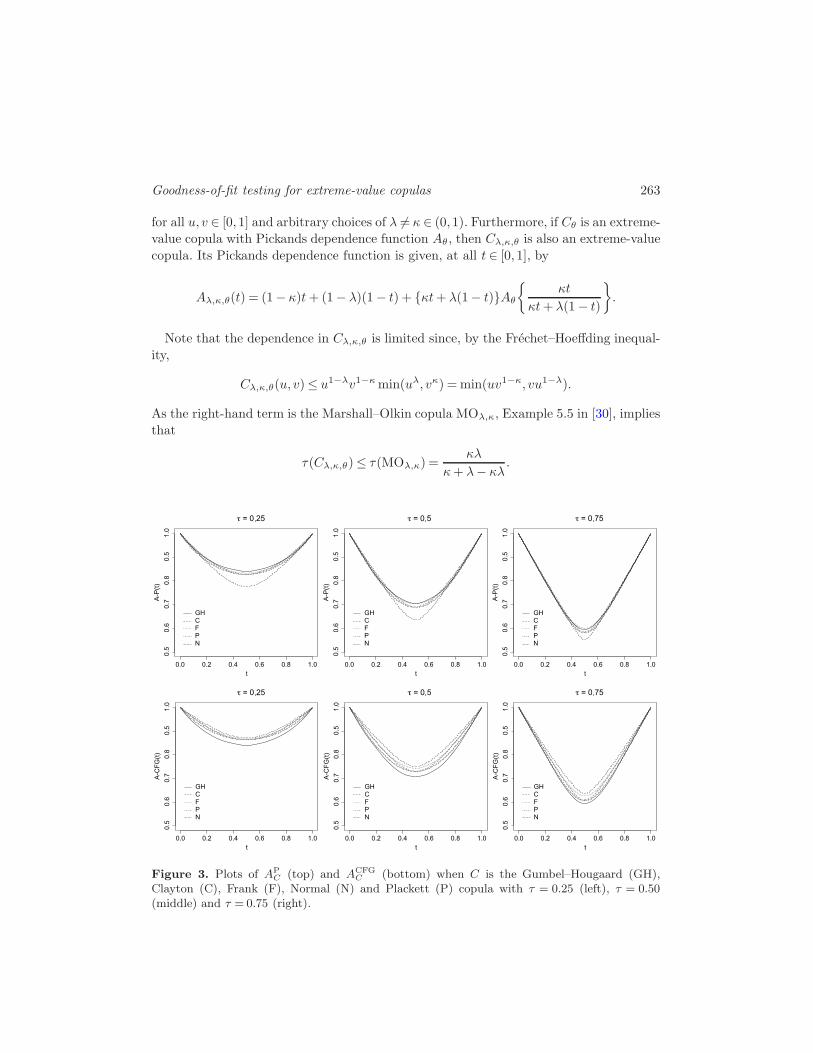
for all u, v ∈ [0,1] and arbitrary choices of λ 6= κ ∈ (0,1). Furthermore, if Cθ is an extreme-

value copula with Pickands dependence function Aθ , then Cλ,κ,θ is also an extreme-value

copula. Its Pickands dependence function is given, at all t ∈ [0,1], by

Aλ,κ,θ(t) = (1− κ)t+ (1− λ)(1− t) + {κt+ λ(1− t)}Aθ

{

κt

κt+ λ(1− t)

}

.

Note that the dependence in Cλ,κ,θ is limited since, by the Frechet–Hoeffding inequal-

ity,

Cλ,κ,θ(u, v)≤ u1−λv1−κmin(uλ, vκ) =min(uv1−κ, vu1−λ).

As the right-hand term is the Marshall–Olkin copula MOλ,κ, Example 5.5 in [30], implies

that

τ(Cλ,κ,θ)≤ τ(MOλ,κ) =κλ

κ+ λ− κλ.

Figure 3. Plots of AP

C (top) and ACFG

C (bottom) when C is the Gumbel–Hougaard (GH),Clayton (C), Frank (F), Normal (N) and Plackett (P) copula with τ = 0.25 (left), τ = 0.50(middle) and τ = 0.75 (right).

264 Genest, Kojadinovic, Neslehova and Yan

Figure 4. Pickands dependence functions for the Gumbel–Hougaard copula and four asymmet-ric extreme-value copulas with τ = 0.20: the asymmetric Gumbel–Hougaard (a-GH), Galambos(a-GA), Husler–Reiss (a-HR) and t-EV (a-t-EV) with four degrees of freedom.

In the present study, the values λ= 0.3, κ= 0.8 were used and, hence, τ(Cλ,κ,θ) couldnot exceed 0.279. For each choice of copula family Cθ in Group III, the parameter θ wasset to make Kendall’s tau equal to 0.20.Figure 4 shows that the Pickands dependence functions of the copulas in Group III

are very similar, though distinct. They are, however, easily distinguished from theirsymmetric counterparts with the same value of tau. Thus, although these extreme-valuecopulas would be difficult to tell apart on the basis of Sn in moderate samples, the testmay still be reasonably powerful against copulas in Group I.

6.2. Monte Carlo study

The observations in Section 6.1 were confirmed through simulations. To this end, 1000random samples of size n= 300 were generated from 28 different copulas, C, correspond-ing to the following scenarios:

(a) C belongs to Group I or II and τ(C) ∈ {0.25,0.50,0.75};(b) C belongs to Group III and τ(C) = 0.20.

The statistics SPn and SCFG

n were computed for each data set. Four hypotheses of the formH0 :A ∈A were then tested. The choices for A were the families of Pickands dependencefunctions for extreme-value copulas in Group I.All tests were carried out at the 5% level. Each P -value was computed on the basis of

N = 1000 parametric bootstrap samples. For comparison purposes, goodness of fit wasalso checked with the general purpose statistic

Tn =

n∑

i=1

|Cn(Ui, Vi)−Cθn(Ui, Vi)|2.

Goodness-of-fit testing for extreme-value copulas 265

Table 1. Percentage of rejection of H0 for copulas in Group I when n= 300

H0 True τ = 0.25 τ = 0.50 τ = 0.75

Tn SPn SCFG

n Tn SPn SCFG

n Tn SPn SCFG

n

GH GH 4.2 3.8 4.0 4.0 4.8 3.6 4.2 5.3 5.5

GA 4.8 4.3 4.2 4.4 3.8 3.8 4.8 4.3 4.3HR 4.8 4.2 4.0 5.4 3.4 3.9 3.7 3.1 1.7t-EV 4.2 3.8 4.5 5.1 5.5 6.4 4.8 7.5 8.9

GA GH 4.5 4.7 3.9 4.0 5.8 4.7 4.4 5.6 6.8GA 4.3 4.6 4.0 5.5 3.9 4.8 4.3 4.7 4.6

HR 4.6 4.8 4.2 5.0 3.4 3.4 3.7 3.7 1.8t-EV 4.6 4.7 4.4 5.3 8.0 7.1 5.7 8.2 10.9

HR GH 4.6 6.4 4.4 4.3 9.6 7.5 4.5 9.6 15.7GA 4.3 5.4 4.5 5.1 6.6 7.2 5.1 8.4 11.7HR 4.9 5.2 4.2 5.3 4.3 3.9 4.0 4.3 3.3

t-EV 4.6 5.9 4.8 5.8 13.7 11.5 6.6 14.9 29.3

t-EV GH 4.2 3.4 4.0 4.1 3.9 2.9 4.0 3.3 2.4GA 4.1 4.3 4.4 4.8 3.4 3.9 4.6 3.0 1.7HR 4.7 4.1 4.4 5.4 3.2 3.4 3.8 2.2 1.3t-EV 4.6 3.7 4.2 4.7 4.8 5.2 4.1 4.3 4.7

This particular test statistic was chosen because of its good overall performance in thelarge scale simulation studies of Berg [2] and Genest et al. [18].Tables 1–4 report the percentages of rejection of the four null hypotheses under each

scenario. Although this made little difference, these results are for the end-point-correctedversions of AP

n and ACFGn , defined for all t ∈ [0,1] by

1/APn,c(t) = 1/AP

n(t)− (1− t){1/APn(0)− 1}− t{1/AP

n(1)− 1}

and

logACFGn,c (t) = log{ACFG

n (t)} − (1− t) log{ACFGn (0)} − t log{ACFG

n (1)}.Before commenting on the results, note that for copulas in Groups I and II, the real-

valued dependence parameter of each data set was estimated by inversion of Kendall’stau; its implementation relied on the numerical approximation technique of Kojadinovicand Yan [26]. For copulas in Group III, which involve several parameters, maximumpseudo-likelihood estimation was used [14, 35].

6.3. Results

It is clear from Table 1 that when n= 300, the tests based on Tn, SPn and SCFG

n cannotdistinguish between copulas in Group I. When τ = 0.25, all rejection rates are within

266 Genest, Kojadinovic, Neslehova and Yan

Table 2. Percentage of rejection of H0 for copulas in Group I when n= 1000

H0 True τ = 0.25 τ = 0.50 τ = 0.75

Tn SPn SCFG

n Tn SPn SCFG

n Tn SPn SCFG

n

GH GH 4.9 4.7 5.3 4.0 5.9 6.0 3.8 5.2 5.4

GA 5.1 5.8 4.0 5.9 4.4 5.1 4.8 3.8 4.2HR 5.1 6.3 6.3 5.1 6.3 9.0 3.4 3.5 9.2t-EV 5.4 4.4 5.4 6.1 6.2 6.9 5.4 9.8 15.9

GA GH 5.2 7.4 6.1 4.4 8.1 8.4 4.3 5.6 7.3GA 5.0 5.6 4.0 5.4 5.1 5.4 4.8 4.4 5.2

HR 4.4 5.0 5.2 4.5 4.5 6.2 3.5 3.1 6.2t-EV 6.1 6.9 6.6 6.7 9.4 12.7 5.5 12.8 23.1

HR GH 6.2 10.6 8.6 5.1 17.6 17.8 5.5 18.1 40.2GA 5.4 6.6 4.1 5.6 8.1 8.8 5.5 12.7 23.4HR 4.6 5.9 5.5 4.2 4.9 5.1 3.4 4.7 5.6

t-EV 6.6 10.1 8.2 8.2 27.0 34.4 6.5 45.2 81.7

t-EV GH 4.7 4.7 5.3 4.4 4.4 5.7 4.0 3.4 3.0GA 4.8 5.6 4.2 5.6 4.8 6.0 4.8 3.0 3.7HR 5.3 6.4 6.1 5.5 8.5 12.3 4.3 3.9 28.7t-EV 5.1 4.5 5.5 5.6 4.8 5.3 5.2 4.5 4.7

sampling error from the nominal level. There are only small signs of improvement as τrises to 0.50 and 0.75. The best scores are obtained when testing for the Husler–Reissmodel with SCFG

n when τ = 0.75. Globally, there is little to choose between the tests.Table 2 shows what happens when n = 1000. Power is on the rise, especially when

τ = 0.75. In the latter case, it seems preferable to base the test on SCFGn rather than on

SPn – both do better than the test based on Tn. Overall, the results remain disappointingly

low, except when testing for the Husler–Reiss model with τ ≥ 0.50.These observations are in line with Figure 2, which shows striking similarities between

the Gumbel–Hougaard, Galambos, Husler–Reiss and t-EV copula with four degrees offreedom. While SP

n and SCFGn still have difficulty telling them apart when the sample

size is 1000, their power eventually rises when n → ∞, as explained in Section 5. Toillustrate this point, samples of various sizes were generated from the Gumbel–Hougaardcopula with τ = 0.50 and the statistic SCFG

n was used to test for the Galambos family.The following results, based on 1000 repetitions and N = 1000 bootstrap samples, givean idea of the sample sizes needed to differentiate models in Group I:

Sample size n 5 000 10 000 20 000 40 000

Percentage of rejection of H0 10.8 22.6 60.2 97.3

Returning to the case n= 300, we can see from Table 3 that the test based on SCFGn

is quite good at detecting non-extreme-value LTD alternatives from Group II. Its power

Goodness-of-fit testing for extreme-value copulas 267

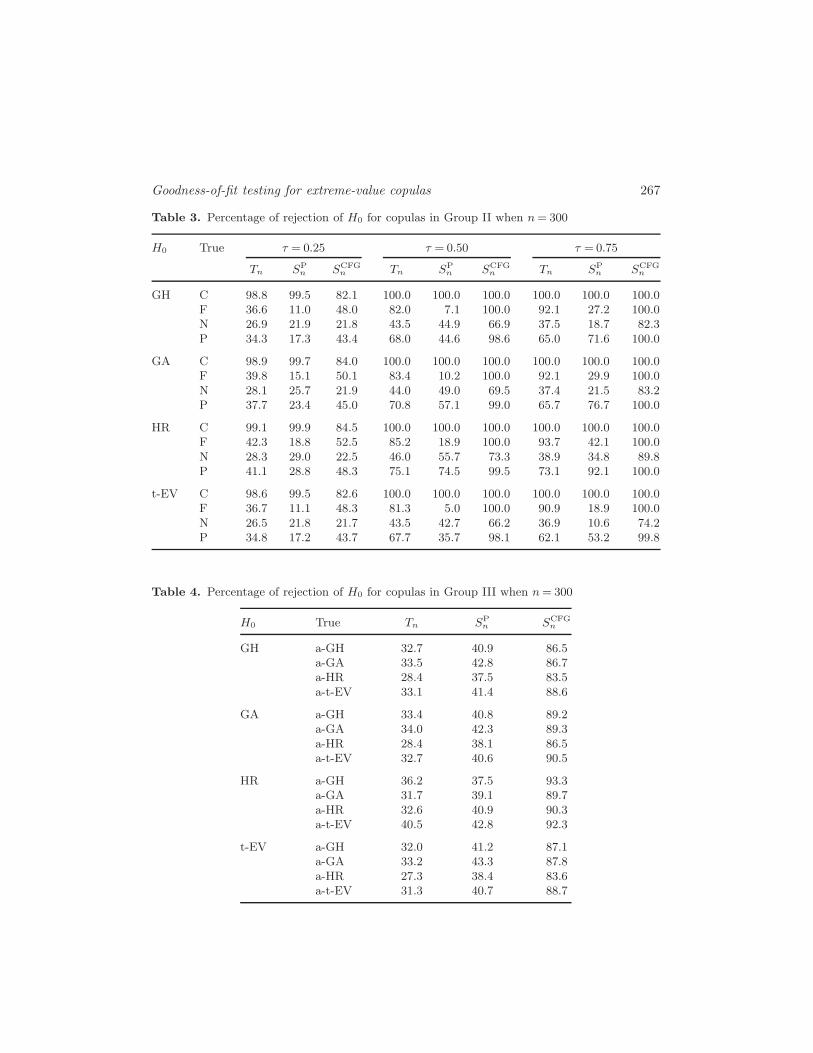
Table 3. Percentage of rejection of H0 for copulas in Group II when n= 300

H0 True τ = 0.25 τ = 0.50 τ = 0.75

Tn SPn SCFG

n Tn SPn SCFG

n Tn SPn SCFG

n

GH C 98.8 99.5 82.1 100.0 100.0 100.0 100.0 100.0 100.0F 36.6 11.0 48.0 82.0 7.1 100.0 92.1 27.2 100.0N 26.9 21.9 21.8 43.5 44.9 66.9 37.5 18.7 82.3P 34.3 17.3 43.4 68.0 44.6 98.6 65.0 71.6 100.0

GA C 98.9 99.7 84.0 100.0 100.0 100.0 100.0 100.0 100.0F 39.8 15.1 50.1 83.4 10.2 100.0 92.1 29.9 100.0N 28.1 25.7 21.9 44.0 49.0 69.5 37.4 21.5 83.2P 37.7 23.4 45.0 70.8 57.1 99.0 65.7 76.7 100.0

HR C 99.1 99.9 84.5 100.0 100.0 100.0 100.0 100.0 100.0F 42.3 18.8 52.5 85.2 18.9 100.0 93.7 42.1 100.0N 28.3 29.0 22.5 46.0 55.7 73.3 38.9 34.8 89.8P 41.1 28.8 48.3 75.1 74.5 99.5 73.1 92.1 100.0

t-EV C 98.6 99.5 82.6 100.0 100.0 100.0 100.0 100.0 100.0F 36.7 11.1 48.3 81.3 5.0 100.0 90.9 18.9 100.0N 26.5 21.8 21.7 43.5 42.7 66.2 36.9 10.6 74.2P 34.8 17.2 43.7 67.7 35.7 98.1 62.1 53.2 99.8

Table 4. Percentage of rejection of H0 for copulas in Group III when n= 300

H0 True Tn SPn SCFG

n

GH a-GH 32.7 40.9 86.5a-GA 33.5 42.8 86.7a-HR 28.4 37.5 83.5a-t-EV 33.1 41.4 88.6

GA a-GH 33.4 40.8 89.2a-GA 34.0 42.3 89.3a-HR 28.4 38.1 86.5a-t-EV 32.7 40.6 90.5

HR a-GH 36.2 37.5 93.3a-GA 31.7 39.1 89.7a-HR 32.6 40.9 90.3a-t-EV 40.5 42.8 92.3

t-EV a-GH 32.0 41.2 87.1a-GA 33.2 43.3 87.8a-HR 27.3 38.4 83.6a-t-EV 31.3 40.7 88.7

268 Genest, Kojadinovic, Neslehova and Yan

is higher than those of SPn and Tn, except when the data are generated from the Clayton

or the Normal copula with τ = 0.25. Interestingly, the general purpose test based on Tn

is often second best. The statistic SPn has the edge only for the Clayton when τ = 0.25;

it does very poorly against the Frank, and against the Normal when τ = 0.75.These results are in close agreement with the plots displayed in Figure 3. Consider, for

instance, the case where SPn is used to test for the Gumbel–Hougaard copula from weakly

dependent data (τ = 0.25). From Table 3, the alternatives can be ranked as follows indecreasing order of power:

Clayton ≻ Normal ≻ Plackett ≻ Frank.

Looking at Figure 3, we find that this ordering is concordant with the overall degree ofdissimilarity between AP

C and A. In this case, as in others, it is found that at fixed samplesize, curves that look alike are harder to distinguish than others.Finally, Table 4 shows that the statistic SCFG

n is much better than the other two atdetecting asymmetric extreme-value alternatives. The overall good performance of thistest is consistent with evidence from [19] that ACFG

n is generally a better nonparametricestimator of the Pickands dependence function than AP

n . When the margins are known,this phenomenon is well documented; see, for example, [4, 22] or [32].

7. Conclusion

Copula models are now common. As illustrated, for instance, by Ben Ghorbal et al.[1], so are situations in which the dependence structure of a random pair (X,Y ) iswell represented by an extreme-value copula, even though X and Y themselves do notnecessarily exhibit extreme-value behavior. In such cases, the statistics considered herecan be used to test the goodness of fit of specific parametric copula families of the form(2) such as the Gumbel–Hougaard, Galambos, Husler–Reiss or Student extreme-valuecopula.Theoretical and empirical evidence presented here shows that the nonparametric tests

based on the Cramer–von Mises statistic Sn are generally consistent and that they arean effective tool for distinguishing between symmetric and asymmetric extreme-valuecopulas, as well as for detecting other left-tail decreasing (LTD) dependence structures.Except in the presence of massive data, however, it seems very difficult to discriminate

between extreme-value copulas whose Pickands dependence functions are close. This maycome as something of a disappointment, but, on reflection, we may wonder whether, inthe light of Figure 2, there is any practical difference between, say, the Gumbel–Hougaardand the Galambos copula when they have the same value of Kendall’s tau.For example, many studies have concluded that a Gumbel–Hougaard copula structure

is adequate for the insurance data mentioned in the Introduction; see, for instance, [5,8, 9, 11, 15, 16] or [27]. In these papers, comparisons were made between the Gumbel–Hougaard model and non-extreme-value copulas that were either Archimedean or meta-elliptical.

Goodness-of-fit testing for extreme-value copulas 269

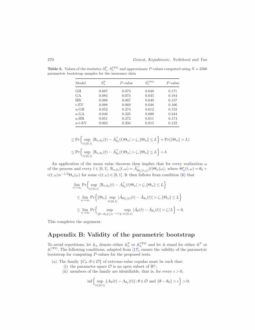
As Ben Ghorbal et al. [1] conclude that the data exhibit extreme-value dependence,it may be worth comparing the Gumbel–Hougaard structure with other extreme-valuecopulas from Groups I and III. This is done in Table 5 using the statistics SP

n and SCFGn

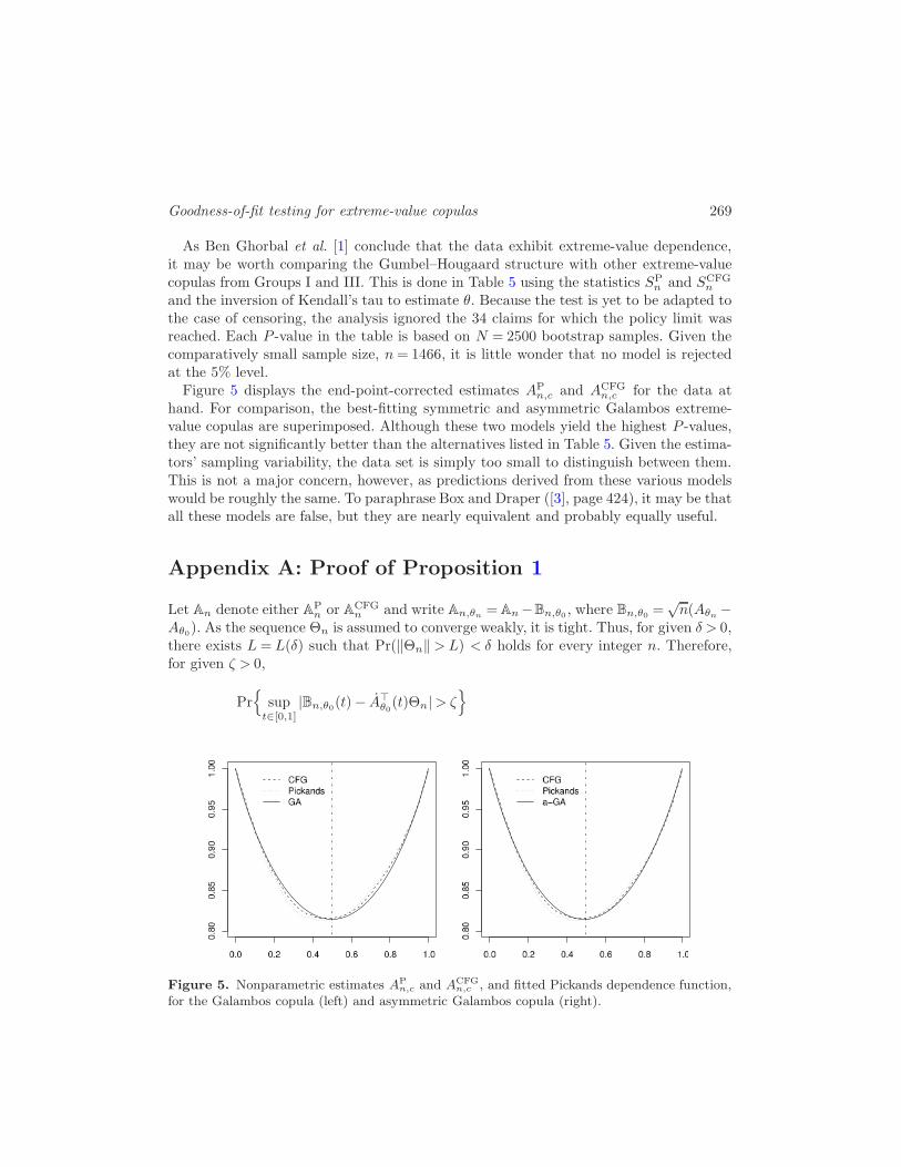
and the inversion of Kendall’s tau to estimate θ. Because the test is yet to be adapted tothe case of censoring, the analysis ignored the 34 claims for which the policy limit wasreached. Each P -value in the table is based on N = 2500 bootstrap samples. Given thecomparatively small sample size, n= 1466, it is little wonder that no model is rejectedat the 5% level.Figure 5 displays the end-point-corrected estimates AP

n,c and ACFGn,c for the data at

hand. For comparison, the best-fitting symmetric and asymmetric Galambos extreme-value copulas are superimposed. Although these two models yield the highest P -values,they are not significantly better than the alternatives listed in Table 5. Given the estima-tors’ sampling variability, the data set is simply too small to distinguish between them.This is not a major concern, however, as predictions derived from these various modelswould be roughly the same. To paraphrase Box and Draper ([3], page 424), it may be thatall these models are false, but they are nearly equivalent and probably equally useful.

Appendix A: Proof of Proposition 1

Let An denote either APn or ACFG

n and write An,θn =An−Bn,θ0 , where Bn,θ0 =√n(Aθn −

Aθ0). As the sequence Θn is assumed to converge weakly, it is tight. Thus, for given δ > 0,there exists L = L(δ) such that Pr(‖Θn‖> L) < δ holds for every integer n. Therefore,for given ζ > 0,

Pr{

supt∈[0,1]

|Bn,θ0(t)− A⊤θ0(t)Θn|> ζ

}

Figure 5. Nonparametric estimates APn,c and ACFG

n,c , and fitted Pickands dependence function,for the Galambos copula (left) and asymmetric Galambos copula (right).

270 Genest, Kojadinovic, Neslehova and Yan

Table 5. Values of the statistics SPn , S

CFGn and approximate P -values computed using N = 2500

parametric bootstrap samples for the insurance data

Model SPn P -value SCFG

n P -value

GH 0.087 0.073 0.048 0.171GA 0.084 0.074 0.045 0.184HR 0.088 0.067 0.049 0.157t-EV 0.088 0.069 0.048 0.166a-GH 0.052 0.274 0.012 0.152a-GA 0.046 0.325 0.009 0.244a-HR 0.051 0.272 0.011 0.174a-t-EV 0.062 0.204 0.015 0.122

≤ Pr{

supt∈[0,1]

|Bn,θ0(t)− A⊤θ0(t)Θn|> ζ,‖Θn‖ ≤ L

}

+Pr(‖Θn‖>L)

≤ Pr{

supt∈[0,1]

|Bn,θ0(t)− A⊤θ0(t)Θn|> ζ,‖Θn‖ ≤ L

}

+ δ.

An application of the mean value theorem then implies that for every realization ωof the process and every t ∈ [0,1], Bn,θ0(t, ω) = A⊤

Θ∗

n(t,ω)(t)Θn(ω), where Θ∗n(t, ω) = θ0 +

ǫ(t, ω)n−1/2Θn(ω) for some ǫ(t, ω)∈ [0,1]. It then follows from condition (6) that

limn→∞

Pr{

supt∈[0,1]

|Bn,θ0(t)− A⊤θ0(t)Θn|> ζ,‖Θn‖ ≤ L

}

≤ limn→∞

Pr{

‖Θn‖ supt∈[0,1]

|AΘ∗

n(t)(t)− Aθ0(t)|> ζ,‖Θn‖ ≤ L

}

≤ limn→∞

Pr{

sup‖θ−θ0‖≤n−1/2L

supt∈[0,1]

|Aθ(t)− Aθ0(t)|> ζ/L}

= 0.

This completes the argument.

Appendix B: Validity of the parametric bootstrap

To avoid repetitions, let An denote either APn or ACFG

n and let A stand for either AP orA

CFG. The following conditions, adapted from [17], ensure the validity of the parametricbootstrap for computing P -values for the proposed tests.

(a) The family {Cθ : θ ∈O} of extreme-value copulas must be such that:(i) the parameter space O is an open subset of Rp;(ii) members of the family are identifiable, that is, for every ǫ > 0,

inf{

supt∈[0,1]

‖Aθ(t)−Aθ0(t)‖ : θ ∈O and ‖θ− θ0‖> ǫ}

> 0;

Goodness-of-fit testing for extreme-value copulas 271

(iii) the mapping θ 7→ Aθ is Frechet differentiable with derivative θ 7→ Aθ , thatis, for all θ0 ∈O,

lim‖h‖↓0

supt∈[0,1]

‖Aθ0+h(t)−Aθ0(t)− A⊤θ0(t)h‖

‖h‖ = 0;

(iv) Cθ has a Lebesgue density cθ for all θ ∈O;(v) the density cθ admits first- and second-order derivatives with respect to all

components of θ ∈O; the gradient (row) vector with respect to θ is denotedcθ and the Hessian matrix is denoted cθ;

(vi) for arbitrary (u, v) ∈ (0,1)2 and every θ0 ∈O, θ 7→ cθ(u, v)/cθ(u, v) and θ 7→cθ(u, v)/cθ(u, v) are continuous at θ0, Cθ0 almost surely;

(vii) for every θ0 ∈ O, there exist a neighborhood N of θ0 and a Lebesgue inte-grable function h : (0,1)2 →R such that supθ∈N ‖cθ(u, v)‖ ≤ h(u, v) holds forall (u, v) ∈ (0,1)2;

(viii) for every θ0 ∈ O, there exist a neighborhood N of θ0 and Cθ0 -integrablefunctions h1, h2 : (0,1)

2 →R such that for all (u, v) ∈ (0,1)2,

supθ∈N

∥

∥

∥

∥

cθ(u, v)

cθ(u, v)

∥

∥

∥

∥

2

≤ h1(u, v) and supθ∈N

∥

∥

∥

∥

cθ(u, v)

cθ(u, v)

∥

∥

∥

∥

≤ h2(u, v).

(b) In addition, the estimators An and θn satisfy the following:(i) (An,Θn,Wn) (A,Θ,W) in D([0,1],R)×Rp⊗2 as n→∞, where the limit is

a centered Gaussian process. Here,

Wn = n−1/2n∑

i=1

c⊤θ0(U∗i , V

∗i )

cθ0(U∗i , V

∗i )

for a random sample (U∗1 , V

∗1 ), . . . , (U

∗n, V

∗n ) from Cθ0 and W is N (0, IP ), where

IP is the Fisher information matrix; see [17], page 1101.(ii) Eθ0(ΘW⊤) = J , where J is the p× p identity matrix. Further, Eθ0{A(t)W}=

Aθ0(t) for every t ∈ (0,1).

Condition (b) can be checked as follows, under the assumption that (An,Θn) (A,Θ)as n → ∞. First, results from Chapter 5 of [12] can be combined with the functionaldelta method (see, e.g., [37], Section 3.9) to see that as n → ∞, (An,Θn,Cn,Wn) (A,Θ,C,W).Next, observe that Eθ0{C(u, v)W} = Cθ0(u, v) for all u, v ∈ [0,1]; see [17], page 1108.

Given that, for all t ∈ [0,1],

AP(t) =−A2

θ0(t)

∫ 1

0

Cθ0(x1−t, xt)

dx

x

and

ACFG(t) =Aθ0(t)

∫ 1

0

Cθ0(x1−t, xt)

dx

x log(x),

272 Genest, Kojadinovic, Neslehova and Yan

we can see that

Eθ0{AP(t)W}=−A2θ0(t)

∫ 1

0

Cθ0(x1−t, xt)

dx

x

and

Eθ0{ACFG(t)W}=Aθ0(t)

∫ 1

0

Cθ0(x1−t, xt)

dx

x log(x).

Interchanging the order of differentiation and integration, we get Eθ0{AP(t)W} =Eθ0{ACFG(t)W}= Aθ0(t) for all t ∈ (0,1).As for the condition Eθ0(ΘW) = J , it can be verified using [17], Proposition 4, for

the estimators based on maximum pseudo-likelihood and on the inversion of Spearman’srho. To handle the estimator based on Kendall’s tau, Proposition 5 in [17] must be usedinstead.

Appendix C: Proof of Proposition 2

The proof closely mimics the argument presented in [19], Appendix B. To avoid dupli-cation, the same notation is used and only the critical differences are highlighted. Thisalso offers an opportunity to correct minor typographical errors in the original source.First, consider the process given by BP

n(t) = n1/2{1/APn(t)− 1/AP

C(t)} for all t ∈ [0,1]and show that BP

n B=−APC/(A

PC)

2 as n→∞. Then

√n(AP

n −APC) =

−(APC)

2BPn

1+ n−1/2BPnA

PC

APC ,

as a consequence of the functional version of Slutsky’s lemma.Put kn = 2 log(n+ 1) and write

BPn(t) =

∫ 1

0

Cn(x1−t, xt)

dx

x=

∫ ∞

0

Cn(e−s(1−t), e−st) ds= I1,n + I2,n,

where, for each t ∈ [0,1],

I1,n(t) =

∫ ∞

kn

Cn(e−s(1−t), e−st) ds, I2,n(t) =

∫ kn

0

Cn(e−s(1−t), e−st) ds.

The contribution of I1,n(t) is asymptotically negligible because the fact that s > knimplies that min(e−s(1−t), e−st)< 1/(n+1) and hence that

|Cn(e−s(1−t), e−st)|= n1/2C(e−s(1−t), e−st)≤ n1/2min(e−s(1−t), e−st)≤ n1/2e−s/2.

Thus, for all t ∈ [0,1],

|I1,n(t)| ≤ n1/2

∫ ∞

kn

C(e−s(1−t), e−st)ds≤ n1/2

∫ ∞

kn

e−s/2 ds≤ 2

n1/2. (A.1)

Goodness-of-fit testing for extreme-value copulas 273

Consequently, the asymptotic behavior of BPn is determined entirely by I2,n. Invoking

the Stute representation given by Genest and Segers [19], we may write I2,n = J1,n +J2,n + J3,n +o(1), where, for each t ∈ [0,1],

J1,n(t) =

∫ kn

0

αn(e−s(1−t), e−st) ds,

J2,n(t) = −∫ kn

0

αn(e−s(1−t),1)C1(e

−s(1−t), e−st) ds,

J3,n(t) = −∫ kn

0

αn(1, e−st)C2(e

−s(1−t), e−st) ds.

Here, C1(u, v) = ∂C(u, v)/∂u, C2(u, v) = ∂C(u, v)/∂v and αn is the empirical processassociated with the pairs (F (X1),G(Y1)), . . . , (F (Xn),G(Yn)).Fix ω ∈ (0,1/2) and write qω(t) = tω(1− t)ω for all t ∈ [0,1]. Also, let

K1(s, t) = qω{min(e−s(1−t), e−st)},K2(s, t) = qω(e

−s(1−t))C1(e−s(1−t), e−st),

K3(s, t) = qω(e−st)C2(e

−s(1−t), e−st)

for all s ∈ (0,∞) and t ∈ [0,1]. The proof that J1,n + J2,n + J3,n has the stated limitthen proceeds exactly as in Appendix B of [19], provided that for i= 1,2,3, there existsan integrable function K∗

i : (0,∞)→ R such that Ki(s, t)≤K∗i (s) for all s ∈ (0,∞) and

t ∈ [0,1].For K1, this is immediate because K1(s, t)≤ e−ωs/2 for all s ∈ (0,∞) and t ∈ [0,1]. For

K2, the facts that C is LTD and smaller than the Frechet–Hoeffding upper bound implythat

C1(e−s(1−t), e−st)≤ es(1−t)C(e−s(1−t), e−st)≤ es(1−t)min(e−s(1−t), e−st).

Now, set m(t) = max(t,1 − t) and note that qω(e−s(1−t)) ≤ e−ωs(1−t) for all s ∈ (0,∞)

and t ∈ [0,1]. Therefore,

K2(s, t)≤ es(1−ω)(1−t)e−sm(t) ≤ es(1−ω)m(t)e−sm(t) = e−sωm(t) ≤ e−ωs/2

because m(t)≥ 1/2 for all t ∈ [0,1]. The argument for K3 is similar.Turning to the ACFG

n estimator, observe that

BCFGn (t) = n1/2{logACFG

n (t)− logACFGC (t)}

=

∫ 1

0

Cn(x1−t, xt)

dx

x log(x)=−

∫ ∞

0

Cn(e−s(1−t), e−st)

ds

s

274 Genest, Kojadinovic, Neslehova and Yan

for all t ∈ [0,1]. This process can be written as −(I1,n + I2,n + I3,n), where

I1,n(t) =

∫ ∞

kn

Cn(e−s(1−t), e−st)

ds

s,

I2,n(t) =

∫ kn

ℓn

Cn(e−s(1−t), e−st)

ds

s,

I3,n(t) =

∫ ℓn

0

Cn(e−s(1−t), e−st)

ds

s

with kn = 2 log(n+1) as above and ℓn = 1/(n+ 1).Arguing as in (A.1), we see that |I1,n| ≤ n−1/2. Similarly, I3,n is negligible asymptoti-

cally, for if s ∈ (0, ℓn) and t ∈ [0,1], then we have

min(e−s(1−t), e−st)≥ e−1/(n+1) >n

n+ 1

and hence Cn(e−s(1−t), e−st) = 1. Furthermore, the fact that C is LTD implies that

C(e−s(1−t), e−st)≥ e−s for all s ∈ (0,∞) and t ∈ [0,1]. Therefore,

|Cn(e−s(1−t), e−st)| ≤ n1/2(1− e−s)≤ n1/2s.

Consequently, |I3,n| ≤ n1/2ℓn ≤ n−1/2. As a result, the asymptotic behavior of BCFGn

is determined entirely by I2,n. Following Genest and Segers [19], we can further writeI2,n = J1,n + J2,n + J3,n + o(1), where, for all t ∈ [0,1],

J1,n(t) =

∫ kn

ℓn

αn(e−s(1−t), e−st)

ds

s,

J2,n(t) = −∫ kn

ℓn

αn(e−s(1−t),1)C1(e

−s(1−t), e−st)ds

s,

J3,n(t) = −∫ kn

ℓn

αn(1, e−st)C2(e

−s(1−t), e−st)ds

s.

The joint asymptotic behavior of these terms can be determined in the same way asbefore. The only difference is that the integration measure is now ds/s. For s ∈ [1,∞),the same upper bounds K∗

1 , K∗2 , K

∗3 apply and they have already been shown to be

integrable on this domain. To obtain an integrable bound for K1 on (0,1), it suffices touse the fact that K1(s, t)≤ (1− e−sm(t))ω ≤ {sm(t)}ω ≤ sω . The same bound works forboth K2 and K3 because Ci ∈ [0,1] for i= 1,2. This completes the argument.

Acknowledgements

This research was supported by grants from the Natural Sciences and Engineering Re-search Council of Canada, the Fonds quebecois de la recherche sur la nature et les tech-

Goodness-of-fit testing for extreme-value copulas 275

nologies, and the Institut de finance mathematique de montreal. Some of the computa-tions were carried out on a Beowulf cluster at the Department of Statistics, Universityof Connecticut, which was partially supported by a grant from the National ScienceFoundation, Scientific Computing Research Environments for the Mathematical Sciences(SCREMS) Program.

References

[1] Ben Ghorbal, N., Genest, C. and Neslehova, J. (2009). On the Ghoudi, Khoudraji, andRivest test for extreme-value dependence. Canad. J. Statist. 37 534–552. MR2588948

[2] Berg, D. (2009). Copula goodness-of-fit testing: An overview and power comparison. Euro-pean J. Finance 15 675–701.

[3] Box, G.E.P. and Draper, N.R. (1987). Empirical Model-Building and Response Surfaces.New York: Wiley. MR0861118

[4] Caperaa, P., Fougeres, A.-L. and Genest, C. (1997). A nonparametric estimation procedurefor bivariate extreme value copulas. Biometrika 84 567–577. MR1603985

[5] Chen, X. and Fan, Y. (2005). Pseudo-likelihood ratio tests for semiparametric multivariatecopula model selection. Canad. J. Statist. 33 389–414. MR2193982

[6] Cherubini, U., Luciano, E. and Vecchiato, W. (2004). Copula Methods in Finance. NewYork: Wiley. MR2250804

[7] Denuit, M., Dhaene, J., Goovaerts, M.J. and Kaas, R. (2005). Actuarial Theory for Depen-dent Risk: Measures, Orders and Models. New York: Wiley.

[8] Denuit, M., Purcaru, O. and Van Keilegom, I. (2006). Bivariate Archimedean copula mod-elling for censored data in nonlife assurance. J. Actuar. Pract. 13 5–32.

[9] Dupuis, D.J. and Jones, B.L. (2006). Multivariate extreme value theory and its usefulnessin understanding risk. N. Am. Actuar. J. 10 1–27. MR2328659

[10] Falk, M. and Reiss, R.-D. (2005). On Pickands coordinates in arbitrary dimensions. J.Multivariate Anal. 92 426–453. MR2107885

[11] Frees, E.W. and Valdez, E.A. (1998). Understanding relationships using copulas. N. Am.Actuar. J. 2 1–25. MR1988432

[12] Ganßler, P. and Stute, W. (1987). Seminar on Empirical Processes. DMV Seminar 9. Basel:Birkhauser. MR0902803

[13] Garralda-Guillem, A.I. (2000). Structure de dependance des lois de valeurs extremes bi-variees. C. R. Acad. Sci. Paris Ser. I Math. 330 593–596. MR1760445

[14] Genest, C., Ghoudi, K. and Rivest, L.-P. (1995). A semiparametric estimation procedure ofdependence parameters in multivariate families of distributions. Biometrika 82 543–552. MR1366280

[15] Genest, C., Ghoudi, K. and Rivest, L.-P. (1998). Discussion of “Understanding relation-ships using copulas,” by E.W. Frees and E.A. Valdez. N. Am. Actuar. J. 2 143–149.MR2011244

[16] Genest, C., Quessy, J.-F. and Remillard, B. (2006). Goodness-of-fit procedures for copulasmodels based on the probability integral transformation. Scand. J. Statist. 33 337–366.MR2279646

[17] Genest, C. and Remillard, B. (2008). Validity of the parametric bootstrap for goodness-of-fit testing in semiparametric models. Ann. Inst. H. Poincare Probab. Statist. 44

1096–1127. MR2469337

276 Genest, Kojadinovic, Neslehova and Yan

[18] Genest, C., Remillard, B. and Beaudoin, D. (2009). Goodness-of-fit tests for copulas: A

review and a power study. Insurance Math. Econom. 44 199–213. MR2517885

[19] Genest, C. and Segers, J. (2009). Rank-based inference for bivariate extreme-value copulas.

Ann. Statist. 37 2990–3022. MR2541453

[20] Ghoudi, K., Khoudraji, A. and Rivest, L.-P. (1998). Proprietes statistiques des copules de

valeurs extremes bidimensionnelles. Canad. J. Statist. 26 187–197. MR1624413

[21] Gudendorf, G. and Segers, J. (2009). Nonparametric estimation of an extreme-value copula

in arbitrary dimensions. Preprint. Available at ArXiv:0910.0845v1.

[22] Hall, P. and Tajvidi, N. (2000). Distribution and dependence-function estimation for bi-

variate extreme-value distributions. Bernoulli 6 835–844. MR1791904

[23] Khoudraji, A. (1995). Contributions a l’etude des copules et a la modelisation des valeurs

extremes bivariees. Ph.D. thesis, Universite Laval, Quebec, Canada.

[24] Kim, G., Silvapulle, M.J. and Silvapulle, P. (2007). Comparison of semiparametric and

parametric methods for estimating copulas. Comput. Statist. Data Anal. 51 2836–2850.

MR2345609

[25] Klugman, S.A. and Parsa, R. (1999). Fitting bivariate loss distributions with copulas.

Insurance Math. Econom. 24 139–148. MR1710816

[26] Kojadinovic, I. and Yan, J. (2010a). Comparison of three semiparametric methods for

estimating dependence parameters in copula models. Insurance Math. Econom. 47

52–63.

[27] Kojadinovic, I. and Yan, J., (2010b). Modeling multivariate distributions with continuous

margins using the copula R package. J. Stat. Software 34 1–20.

[28] Liebscher, E. (2008). Construction of asymmetric multivariate copulas. J. Multivariate

Anal. 99 2234–2250. MR2463386

[29] McNeil, A.J., Frey, R. and Embrechts, P. (2005). Quantitative Risk Management: Concepts,

Techniques, and Tools. Princeton, NJ: Princeton Univ. Press. MR2175089

[30] Nelsen, R.B. (2006). An Introduction to Copulas, 2nd edition. New York: Springer.

MR2197664

[31] Pickands III, J. (1981). Multivariate extreme value distributions. In Proceedings of the 43rd

Session of the International Statistical Institute, Vol. 2 (Buenos Aires, 1981). Bull.

Inst. Internat. Statist. 49 859–878, 894–902. MR0820979

[32] Rojo-Jimenez, J., Villa-Diharce, E. and Flores, M. (2001). Nonparametric estimation of the

dependence function in bivariate extreme value distributions. J. Multivariate Anal. 76

159–191. MR1821817

[33] Ruschendorf, L. (1976). Asymptotic distributions of multivariate rank order statistics. Ann.

Statist 4 912–923. MR0420794

[34] Salvadori, G., De Michele, C., Kottegoda, N.T. and Rosso, R. (2007). Extremes in Nature:

An Approach Using Copulas. New York: Springer.

[35] Shih, J.H. and Louis, T.A. (1995). Inferences on the association parameter in copula models

for bivariate survival data. Biometrics 51 1384–1399. MR1381050

[36] Sklar, A. (1959). Fonctions de repartition a n dimensions et leurs marges. Publ. Inst. Statist.

Univ. Paris 8 229–231. MR0125600

[37] van der Vaart, A.W. and Wellner, J.A. (1996). Weak Convergence and Empirical Processes.

New York: Springer. MR1385671

[38] Yan, J. and Kojadinovic, I. (2009). Copula: Multivariate dependence with copulas. R Pack-

age Version 0.8–12.

Goodness-of-fit testing for extreme-value copulas 277

[39] Zhang, D., Wells, M.T. and Peng, L. (2008). Nonparametric estimation of the dependencefunction for a multivariate extreme value distribution. J. Multivariate Anal. 99 577–588. MR2406072

Received August 2009 and revised January 2010