A Glimpse of Representing Stochastic Processescephil.usask.ca/Classes/CMPT858Fall2012/Lectures/PDFs/Lecture 28... · A Glimpse of Representing Stochastic Processes Nathaniel Osgood

A Glimpse of Representing Stochastic Processes

Nathaniel Osgood

CMPT 858

November 22, 2012

Dynamic Uncertainty: Stochastic Processes

• Examples of things commonly stochastically approximated – Stock market

– Rainfall

– Oil prices

– Economic growth

• What considered “stochastic” will depend on the scope of the model – Detailed model: Individual behaviour, transmission,

differential severity of infection, etc.

– A meteorological model may not consider rainfall stochastic

Stochastic Processes in AnyLogic

• In AnyLogic, ABM and Discrete Event Models (“Network-Based Modeling”) are typically stochastic

– Transitions between states

– Event firing

– Messages

• (Frequent) timing of message send

• Target of messages

– Duration of a procedure

• As a result, there will be variation in the results from simulation to simulation

Summarizing Variability • To gain confidence in model results, typically

need to run a “Monte Carlo” ensemble of realizations

– Deal with means, standard deviations, and empirical fractiles

– As is seen here, there are typically still broad regularities between most runs (e.g. rise & fall)

• Need to reason over a population of realizations statistics are very valuable

– Fractile within which historic value falls

– Mean difference in results between interventions

Monte Carlo Methods in AnyLogic • Monte Carlo methods draw repeated samples from

distributions & stochastic processes of interest

• When running Monte Carlo method, we’d like to summarize the results of multiple runs

• One option would be to display each trajectory over time; downside: quickly gets messy

• AnyLogic’s solution

– Accumulate data regarding how many trajectories fall within given areas of value for a given interval of time using a “Histogram2D Data”

– Display the Histogram2D Chart

MonteCarlo2D Histogram

• Divides up time into user-specified # of intervals

• This forms a set of divisions along the horizontal (time) axis

• Divides up value axis for quantity being displayed into a user-specified # of interval

• This forms a set of divisions along the vertical (value) axis

• Together, the divisions define a uniform (2D) grid

• For each cell on that grid, a “Histogram2D Data” object accumulates data regarding how many trajectories include a value within that cell – i.e. how many trajectories have hold a range of values during a

given interval of time)

Hands on Model Use Ahead

Load Sample Model: SIR Agent Based Calibration

(Via “Sample Models” under “Help” Menu)

Monte Carlo Analysis with Fixed Parameter Values

Results of Monte Carlo Simulation

Even without parameter variation, Substantial variability is still present!

2D Histogram Data

Important Distinction (Declining Order of Aggregation)

• Experiment

– Collection of simulations

• Simulation

– Collection of replications that can yield findings across set of replications (e.g. mean value)

• Replication

– One run of the model

Flexibility Typically Ignored

• In most AnyLogic models, an Experiment is composed of a single Simulation, which is composed of a single Replication

• In most AnyLogic models which run “ensembles” of realizations, a simulation is composed of only a single realization

Accumulating the Histogram2D dataset from other datasets

The source dataset is in Main

The accumulating Histogram2D dataset is in Experiment

Monte Carlo Sensitivity Analyses in AnyLogic

Choice between showing envelopes of empirical fractiles & showing counts in histogram bins

Difference Between Chart Options “Show envelopes”

• This option shows envelopes of empirical fractiles – These are associated with empirical fractiles defined in

terms of percentages (e.g. “0.25” means boundary between lowest and 2nd lowest quartile; “0.50” means median)

– e.g. These define envelopes of (contours) around the median within which data from different % of realizations fall

– A “slice” through the output at a particular moment in time would be like an extended boxplot (showing fractiles)

• The empirical fractiles to use are themselves defined in the associated Histogram2D Data object

Reminder: 2D Histogram Data

Note definition of envelopes to be used in The Histogram2D Chart if “Show envelopes” is selected.

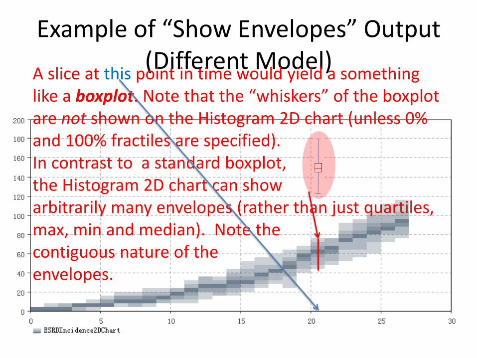
Example of “Show Envelopes” Output (Different Model)

A slice at this point in time would yield a something like a boxplot. Note that the “whiskers” of the boxplot are not shown on the Histogram 2D chart (unless 0% and 100% fractiles are specified). In contrast to a standard boxplot, the Histogram 2D chart can show arbitrarily many envelopes (rather than just quartiles, max, min and median). Note the contiguous nature of the envelopes.

Show Bins Option

The “show bins” option is here.

Example of “Show Bins” Output (Different Model)

A slice at this point in time would yield a histogram. Note: In contrast to the situation for the envelopes (which are contiguous), the “show bins” can exhibit multiple modes.

Automatic Throttling of Monte Carlo Analyses

General Variety of Output

Reminder: Statistical Scaling

• Consider Taking the sample mean of n samples that vary independently around a mean

• If two samples x and y are independent samples of random variables X and Y, then Var[x+y]=Var[X]+Var[Y]

– So if we have n indep. samples xi from distribution X

• If we scale a random variable by a factor , the standard deviation scales by the same factor of => the variance scales by 2

– i.e. StdDev[X]= StdDev[X], Var[X]= 2 Var[X]

1

n

i

i

Var x nVar X

Statistics of Sample Mean

• Recall: Sample Mean:

• From the preceding, variance drops as 1/n

• This means that standard deviation for the sample mean of n samples drops as 1/sqrt(n)

• So if we wish to divide the standard deviation of the sample mean by a factor of 2, we need to take 4x the number of Monte Carlo samples

11

2 2

nn

iiii

Var xxnVar X Var X

Var m Varn n n n

1

n

i

i

x

mn

2

StdDev XVar X StdDev XStdDev m Var m

n n n

Closing Question: How can we best adapt our policies to deal with ongoing uncertainty?

• We are dealing here with making decisions in an environment that changes over time

• This uncertainty could come from – Stochastic variability

– Uncertainty regarding parameter values

• There is an incredibly vast # of possible policies • Reminder: Can successfully integrate decision analysis

& simulation to neatly handle such cases

Baseline50% 60% 70% 80% 90% 95% 98% 100%

Average Variable Cost per Cubic Meter

0.6

0.45

0.3

0.15

00 1457 2914 4371 5828

Time (Day)