A GIS-BASED SYNTHESIS OF INFORMATION ON SPAWNING DISTRIBUTIONS OF CHINOOK SALMON IN THE CALIFORNIA COAST CHINOOK SALMON ESU

NOAA Technical Memorandum NMFS

MAY 2005

A GIS-BASED SYNTHESIS OF INFORMATION ON SPAWNING DISTRIBUTIONS OF CHINOOK SALMON

IN THE CALIFORNIA COAST CHINOOK SALMON ESU

A. Agrawal R. Schick

E. Bjorkstedt B. Spence M. Goslin B. Swart

NOAA-TM-NMFS-SWFSC-377

U.S. DEPARTMENT OF COMMERCE National Oceanic and Atmospheric Administration National Marine Fisheries Service Southwest Fisheries Science Center

NOAA Technical Memorandum NMFS

The National Oceanic and Atmospheric Administration (NOAA), organized in 1970, has evolved into an agency which establishes national policies and manages and conserves our oceanic, coastal, and atmospheric resources. An organizational element within NOAA, the Office of Fisheries is responsible for fisheries policy and the direction of the National Marine Fisheries Service (NMFS).

In addition to its formal publications, the NMFS uses the NOAA Technical

Memorandum series to issue informal scientific and technical publications when complete formal review and editorial processing are not appropriate or feasible. Documents within this series, however, reflect sound professional work and may be referenced in the formal scientific and technical literature.

NOAA Technical Memorandum NMFS This TM series is used for documentation and timely communication of preliminary results, interim reports, or special purpose information. The TMs have not received complete formal review, editorial control, or detailed editing.

MAY 2005

A GIS-BASED SYNTHESIS OF INFORMATION ON SPAWNING DISTRIBUTIONS OF CHINOOK SALMON

IN THE CALIFORNIA COAST CHINOOK SALMON ESU

A. Agrawal1, R. Schick, E. Bjorkstedt, B. Spence, M. Goslin2, B. Swart

Santa Cruz Laboratory Southwest Fisheries Science Center

NOAA National Marine Fisheries Service 110 Shaffer Road

Santa Cruz, CA 95060

1Current Address: Center for GIS Research, California State Polytechnic University, 3801 W. Temple Ave., Pomona, CA 91768

2Current Address: Ecotrust, 721 Ninth Ave., Portland, OR 97209

NOAA-TM-NMFS-SWFSC-377

U.S. DEPARTMENT OF COMMERCE Carlos M. Gutierrez, Secretary National Oceanic and Atmospheric Administration Vice Admiral Conrad C. Lautenbacher, Jr., Under Secretary for Oceans and Atmosphere National Marine Fisheries Service William T. Hogarth, Assistant Administrator for Fisheries

Abstract

This report presents a database of observations assembled from local expertknowledge on the distribution of chinook salmon in the California Coastal Chi-nook Salmon Evolutionarily Significant Unit (CCC ESU). Expert knowledgewas transcribed into a Geographic Information System (GIS) in a spatial for-mat that was easy to interpret, update, and share. The geospatial databaseincludes 499 habitat observations and 119 observations of barriers to fish pas-sage.

1 Introduction

The California Coastal Chinook Salmon Evolutionarily Significant Unit (CCC ESU)

is listed as a threatened species under the Federal Endangered Species Act (ESA).

Estimating the quality and extent of available habitat is necessary for developing

effective plans to restore these depleted populations; however, spatial data on the

spawning distribution of chinook salmon in the CCC ESU are sparse and have not

been assembled previously. Indeed, a lack of this type of information contributed to

the decision to list the species on the ESA (Myers et al. 1998). In an attempt to fill

this gap, we assembled information on the spawning distribution of chinook salmon

throughout the CCC ESU, through a series of mapping exercises involving local ex-

perts. Our steps for this exercise were to (1) gather and assess available information

on chinook distribution in the ESU; (2) synthesize this collected information into a

comprehensive spatial data set using a Geographic Information System (GIS); and

(3) error-check and resolve conflicting comments.

1

2 Methods

2.1 Gathering & Assembling Expert Knowledge

Three meetings were held (8 July 2002 [Arcata, CA], 6 August 2002 [Fortuna, CA],

and 28 August 2002 [Santa Rosa, CA]) to ensure geographic coverage and to facil-

itate participation by a broad range of local experts. The meetings were held in a

collaborative format to encourage participants to resolve discrepancies before pro-

viding opinions. On draft maps at the watershed scale, we asked each expert to

note their initials, reference document if applicable, year of observation, and any ad-

ditional supporting information (e.g., distance from confluence, at road crossing x,

etc.) with each observation. Each draft map depicted 1:100k hydrography (USGS

2003) with watershed boundaries1, roads, and other landscape features to better ori-

ent the participant. These procedures were repeated with all available experts until

all watersheds in the CCC ESU where field surveying had taken place were included.

We developed coding schemes to categorize observations about chinook dis-

tribution according to (1) type (spawning/rearing, rearing/migration, or migration),

(2) data quality class (Documented, Professional Observation, Suspected, Disputed,

Documented but Upper Spatial Extent Unknown), and (3) time scale (Appendix A).

We categorized barrier observations by type and passability (Appendix B).

We digitized the observation data into a GIS using the Dynamic Segmentation

1We developed watershed boundaries so that the bounds encompassed the entire drainage area,which was delineated using 1:100K hydrography (USGS 2003) and sixth-level hydrologic unit bound-aries (FRAP 1999; NRCS 2002). If these ancillary data were insufficient, DEMs were used to visualizeand trace the catchment area.

2

Model (DSM)2, which allowed us to store the data as a set of measurements along the

stream (ESRI 2002)3. Specifically, the DSM allowed for relating linearly referenced

data (events, i.e. Chinook presence), stored as a table, onto linear features (routes, i.e.

rivers) (Cadkin and Brennan 2002). Additionally, the DSM provided the capability

to store overlapping events, which was useful in instances where observations between

experts differed. A different color was used for each type of event according to the

coding schemes.

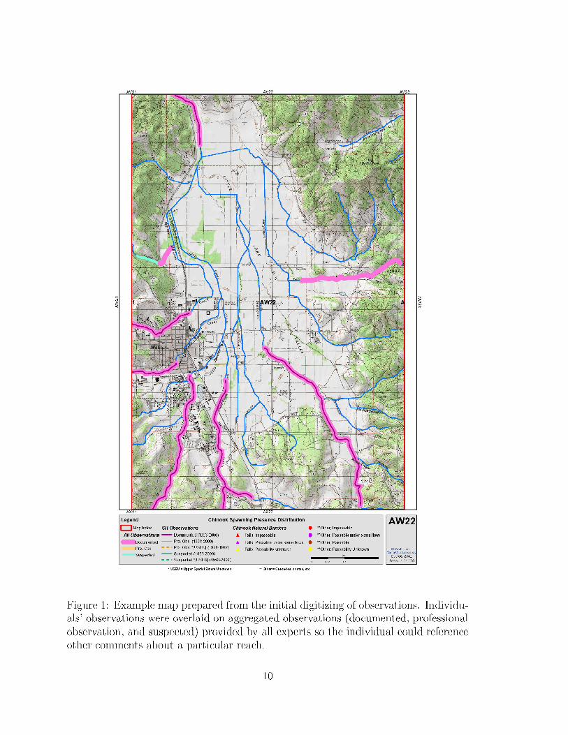
To resolve disputes between experts and locate and remedy any mapping errors,

we developed a series of 1:24k scale maps for all areas with observations. Each map

depicted aggregated observations made by all experts as a base layer with overlays

of observations with all possible categories made by an individual expert (Figure 1).

We used a hierarchical framework for overlapping or disputed observations where

Documented observations took precedence over Professional observations, which took

precedence over Suspected. Additional map layers included topographic maps, 1:100k

2Dynamic Segmentation refers to a method of referencing data along a linear feature such thatmeasurements along the feature are used for location (ESRI 2001). Events refer to each line or pointobservation. For line events (Chinook spawning and rearing), two measurements are needed for thestart and end points of each line. For point events (barriers), one measurement is needed. Routes areany linear feature upon which events can be located (Cadkin and Brennan 2002). We used a 1:100krouted stream coverage (Christy and Haney 2003; downloadable from http://www.calfish.org/) as thebase stream layer upon which we placed georeferenced events. This route system uses a Longitude-Latitude Identifier (LLID)to link each stream to the correct observation. The LLID is the longitudeand latitude coordinates at the mouth or confluence of a stream. We used the Digitize Eventstoolbar (downloadable from http://arcobjectsonline. esri.com/) to digitize each observation. Lastly,we overlayed seamless topographic maps (TOPO 2001) to ensure more accurate digitizing. Thissystem corresponds to similar methodology used in Oregon (Oregon Department of Fish and Wildlife,http://rainbow.dfw.state.or.us/nrimp/24k/docs/workshop.pdf).

3Disclaimer of Endorsement: Reference to any specific commercial products, process, or serviceby trade name, trademark, manufacturer, or otherwise, does not constitute or imply its endorsement,recommendation, or favoring by the United States Government. The views and opinions of authorsexpressed in this document do not necessarily state or reflect those of NOAA or of the United StatesGovernment, and shall not be used for advertising or product endorsement purposes.

3

hydrography, and the barrier data set. Each expert was asked to review all maps for

which they contributed information. To ensure the correct classification and spatial

extent of each observation, we asked each expert to verify each delineation and provide

any comments or needed corrections.

3 Structure and Summary of the Chinook Distri-

bution Database

The databases (downloadable from http://santacruz.nmfs.noaa.gov/publications/ soft-

ware/673) contain 499 events depicting chinook spawning and rearing, and 119 events

depicting barriers to fish passage (Figure 2). Chinook spawning and rearing was re-

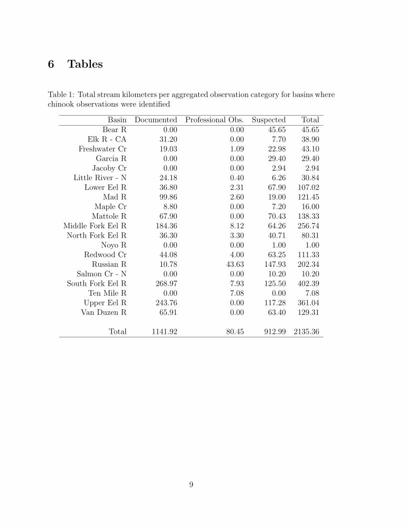
ported in 2135 stream kilometers in the CCC ESU with 53% as Documented, 4%

as Professional Observation, and 43% as Suspected (Table 1). (As noted above, the

databases contains observations that overlap in space and in time, but these tab-

ular results present aggregated data that contain spatially and temporally unique

events.) In addition to these tabular summaries, the observations can be displayed

on watershed level maps by class and time (Figure 3).

Observations were concentrated in the northern portion of the ESU, while

relatively few observations occurred south of the Eel River basin (Figure 2). The

entire Eel River basin accounted for 62% of the total stream kilometers present in

the database. While this patterns appears to reflect the actual distribution of chi-

nook, there may also be some geographic bias in sampling because fewer surveys were

conducted farther south where chinook are though to be much less abundant.

4

The distribution of barriers to chinook passage were more concentrated in

inland portions of larger watersheds. Small, coastal watersheds had few barrier ob-

servations; however, the Little River, one of the smallest watersheds in the ESU,

contained 10 of the total 119 observations (8%). Watersheds with > 10 barrier ob-

servations included the Mad (11), South Fork Eel (13), Russian (15), and Upper Eel

(21). Sixty-two percent of the observed barriers were natural barriers. Eighty-five

percent of all observations were either impassable or only passable under some flows.

The distribution of these observations likely reflects the same geographic bias noted

above.

3.1 Caveats

Some caution should be applied in interpreting these results. First, there are degrees

of subjectivity for some of the observations, which we indicated by data quality classes.

Second, measurements of each delineation or observation were not precise as the data

set was delineated and digitized manually on maps, and therefore there may be small

errors in actual locations and the summarized tabular data. Additionally, as noted in

the preceding section, there appears to be a geographic sampling bias, and therefore

we do not intend to conclude that fish are not distributed in these less or unsampled

areas. Nonetheless, these data provide the best current estimate of the spatial extents

and locations of chinook distribution in the ESU, and can be updated as further

information becomes available.

5

3.2 Potential Applications

These data may be useful for helping develop effective recovery plans in several ways.

We can use these data to guide field surveys in those suspected areas, and in so

doing generate more accurate presence/absence data for the ESU. These data might

also be used to determine population structure within the ESU. Also, these results

can be used as a validation data set for models that predict fish distribution (e.g.

habitat suitability models). For example, we have modeled the intrinsic potential for

fish habitat based on the underlying geomorphology and hydrology (stream gradient,

valley constraint, and discharge) (Burnett et al., 2003; Agrawal et al., In review).

The chinook spatial data that were generated through the mapping exercises can be

used to compare and quantify modeled results.

4 Acknowledgements

We thank the following for their comments and participation in the mapping exer-

cises: Bill Cox (CDFG), Robert Darby (Scotia Pacific Company, LLC), Scott Downie

(CDFG), Michele Gilroy (CDFG), Scott Harris (CDFG), Weldon Jones (CDFG),

David Manning (Sonoma County Water Agency), Brian Michaels (Simpson Timber

Company), Gary Peterson (Mattole Salmon Group), Lawrence G. Preston (CDFG),

Brooks Smith (USDA Forest Service), and Tom Weseloh (CalTrout). We thank Kerrie

Pipal and Dave Rundio for helpful comments on this manuscript.

6

5 References

Agrawal, A., R. Schick, E. Bjorkstedt, R.G. Szerlong, M. Goslin, B. Spence, T.

Williams, and K. Burnett. In review. Predicting the potential for histori-

cal coho, chinook and steelhead habitat in Northern California. NOAA Tech.

Memo.

Burnett, K. M., H. G. H. Reeves, D. Miller, S. E. Clarke, K. C. Christiansen,

and K. Vance-Borland. 2003. A first step toward broad-scale identification

of freshwater protected areas for Pacific salmon and trout. In: J. Beumer

(ed.), Proceedings of the World Congress on Aquatic Protected Areas, Cairns,

Australia, August 14-18, 2002. Australian Society for Fish Biology.

Cadkin, J. and P. Brennan. 2002. Dynamic segmentation in ArcGIS. ArcUser. ESRI

Press, Redlands, CA, July - September.

Christy, T. and E. Haney. 2003. 1:100k hydrography (Version 2003.6). Pacific

States Marine Fisheries Council and California Department of Fish and Game.

http://www.calfish.org/.

ESRI. 2002. Environmental Systems Research Institute ArcGIS 8.3 software. Red-

lands, CA.

ESRI. 2001. Linear referencing and dynamic segmentation in ArcGIS 8.1, an ESRI

white paper. Environmental Systems Research Institute, Redlands, CA, May.

7

FRAP. 1999. California watersheds (CALWATER 2.2). California Department of

Forestry and Fire Protection, Fire and Resource Assessment Program. http://

gis.ca.gov/meta.epl?oid=5298.

Myers, J. M., R. G. Kope, G. J. Bryant, D. Teel, L. J. Lierheimer, T. C. Wain-

wright, W. S. Grant, F. W. Waknitz, K. Neely, S. T. Lindley, and R. S. Waples.

1998. Status review of Chinook salmon from Washington, Idaho, Oregon, and

California. NOAA Technical Memorandum, NMFS-NWFSC-35, 443 p.

NRCS. 2002. 8- 10- and 12- digit HUs for Oregon, Washington, and Northern

California. U. S. Department of Agriculture, Natural Resources Conservation

Service, Titan Geospatial. http://www.gis.state.or.us/.

TOPO. 2001. Topo software version 2.6.8. National Geographic Holdings.

USGS. 2003. National hydrography dataset. U. S. Department of the Interior, U.

S. Geological Survey. http://nhd.usgs.gov/.

8

6 Tables

Table 1: Total stream kilometers per aggregated observation category for basins wherechinook observations were identified

Basin Documented Professional Obs. Suspected TotalBear R 0.00 0.00 45.65 45.65

Elk R - CA 31.20 0.00 7.70 38.90Freshwater Cr 19.03 1.09 22.98 43.10

Garcia R 0.00 0.00 29.40 29.40Jacoby Cr 0.00 0.00 2.94 2.94

Little River - N 24.18 0.40 6.26 30.84Lower Eel R 36.80 2.31 67.90 107.02

Mad R 99.86 2.60 19.00 121.45Maple Cr 8.80 0.00 7.20 16.00

Mattole R 67.90 0.00 70.43 138.33Middle Fork Eel R 184.36 8.12 64.26 256.74North Fork Eel R 36.30 3.30 40.71 80.31

Noyo R 0.00 0.00 1.00 1.00Redwood Cr 44.08 4.00 63.25 111.33

Russian R 10.78 43.63 147.93 202.34Salmon Cr - N 0.00 0.00 10.20 10.20

South Fork Eel R 268.97 7.93 125.50 402.39Ten Mile R 0.00 7.08 0.00 7.08

Upper Eel R 243.76 0.00 117.28 361.04Van Duzen R 65.91 0.00 63.40 129.31

Total 1141.92 80.45 912.99 2135.36

9

Redwood Creek

Maple Creek

Little River - N

Mad RiverJacoby Creek

Freshwater CreekElk River - CA

Salmon Creek - N

Lower Eel RiverGuthrie Creek

Bear River

McNutt Gulch

Mattole River

Usal Creek

South Fork Eel River

Ten Mile River

Noyo River

Big RiverAlbion River

Navarro River

Gualala River

Garcia River

Elk CreekGreenwood Creek

Brush CreekAlder Creek

Russian River

Pudding Creek

Cottaneva Creek

Wages CreekJuan Creek

Van Duzen River

North Fork Eel River

Middle Fork Eel River

Upper Eel River

Big Salmon Creek

Caspar Creek

Chinook Spawning/Rearing ObservationsDocumented

Professional Observation

Suspected

0 260 520130

Kilometers N

Figure 2: Map showing all gathered observations.

11

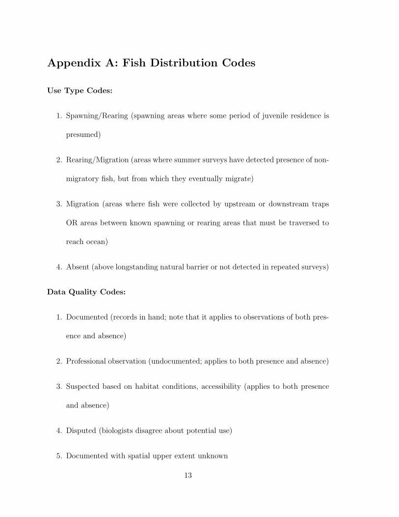
Appendix A: Fish Distribution Codes

Use Type Codes:

1. Spawning/Rearing (spawning areas where some period of juvenile residence is

presumed)

2. Rearing/Migration (areas where summer surveys have detected presence of non-

migratory fish, but from which they eventually migrate)

3. Migration (areas where fish were collected by upstream or downstream traps

OR areas between known spawning or rearing areas that must be traversed to

reach ocean)

4. Absent (above longstanding natural barrier or not detected in repeated surveys)

Data Quality Codes:

1. Documented (records in hand; note that it applies to observations of both pres-

ence and absence)

2. Professional observation (undocumented; applies to both presence and absence)

3. Suspected based on habitat conditions, accessibility (applies to both presence

and absence)

4. Disputed (biologists disagree about potential use)

5. Documented with spatial upper extent unknown

13

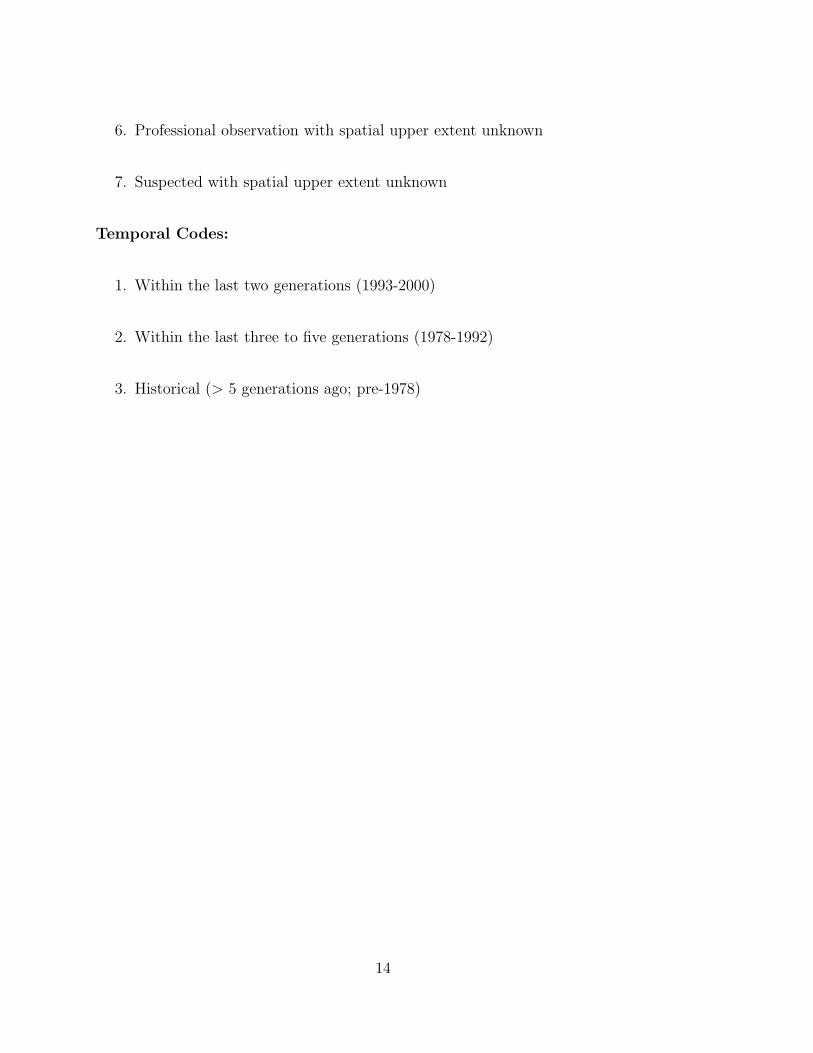
6. Professional observation with spatial upper extent unknown

7. Suspected with spatial upper extent unknown

Temporal Codes:

1. Within the last two generations (1993-2000)

2. Within the last three to five generations (1978-1992)

3. Historical (> 5 generations ago; pre-1978)

14

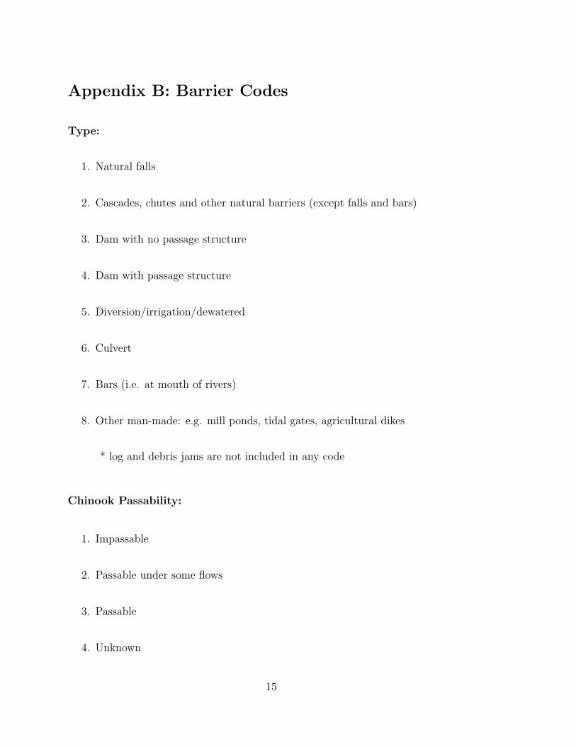
Appendix B: Barrier Codes

Type:

1. Natural falls

2. Cascades, chutes and other natural barriers (except falls and bars)

3. Dam with no passage structure

4. Dam with passage structure

5. Diversion/irrigation/dewatered

6. Culvert

7. Bars (i.e. at mouth of rivers)

8. Other man-made: e.g. mill ponds, tidal gates, agricultural dikes

* log and debris jams are not included in any code

Chinook Passability:

1. Impassable

2. Passable under some flows

3. Passable

4. Unknown

15

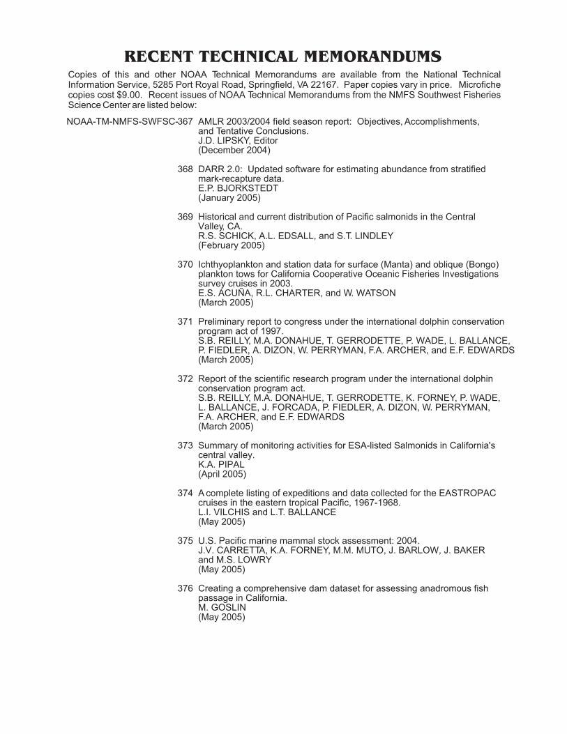
RECENT TECHNICAL MEMORANDUMSCopies of this and other NOAA Technical Memorandums are available from the National Technical Information Service, 5285 Port Royal Road, Springfield, VA 22167. Paper copies vary in price. Microfiche copies cost $9.00. Recent issues of NOAA Technical Memorandums from the NMFS Southwest Fisheries Science Center are listed below:

NOAA-TM-NMFS-SWFSC-367 AMLR 2003/2004 field season report: Objectives, Accomplishments, and Tentative Conclusions. J.D. LIPSKY, Editor (December 2004)

368 DARR 2.0: Updated software for estimating abundance from stratified mark-recapture data. E.P. BJORKSTEDT (January 2005)

369 Historical and current distribution of Pacific salmonids in the Central Valley, CA. R.S. SCHICK, A.L. EDSALL, and S.T. LINDLEY (February 2005)

370 Ichthyoplankton and station data for surface (Manta) and oblique (Bongo) plankton tows for California Cooperative Oceanic Fisheries Investigations survey cruises in 2003. E.S. ACUÑA, R.L. CHARTER, and W. WATSON (March 2005)

371 Preliminary report to congress under the international dolphin conservation program act of 1997. S.B. REILLY, M.A. DONAHUE, T. GERRODETTE, P. WADE, L. BALLANCE, P. FIEDLER, A. DIZON, W. PERRYMAN, F.A. ARCHER, and E.F. EDWARDS (March 2005)

372 Report of the scientific research program under the international dolphin conservation program act. S.B. REILLY, M.A. DONAHUE, T. GERRODETTE, K. FORNEY, P. WADE, L. BALLANCE, J. FORCADA, P. FIEDLER, A. DIZON, W. PERRYMAN, F.A. ARCHER, and E.F. EDWARDS (March 2005)

373 Summary of monitoring activities for ESA-listed Salmonids in California's central valley. K.A. PIPAL (April 2005)

374 A complete listing of expeditions and data collected for the EASTROPAC cruises in the eastern tropical Pacific, 1967-1968. L.I. VILCHIS and L.T. BALLANCE (May 2005)

375 U.S. Pacific marine mammal stock assessment: 2004. J.V. CARRETTA, K.A. FORNEY, M.M. MUTO, J. BARLOW, J. BAKER and M.S. LOWRY (May 2005)

376 Creating a comprehensive dam dataset for assessing anadromous fish passage in California. M. GOSLIN (May 2005)