A Giggle a Minute: Agent-based simulation of laughter propagation in an audience Theresa O’Brien Supervised by Assoc. Prof. Mark Nelson University of Wollongong In Collaboration with Dr. Tristram Alexander University of Sydney Vacation Research Scholarships are funded jointly by the Department of Education and Training and the Australian Mathematical Sciences Institute.

Welcome message from author
This document is posted to help you gain knowledge. Please leave a comment to let me know what you think about it! Share it to your friends and learn new things together.
Transcript
A Giggle a Minute: Agent-based
simulation of laughter propagation in
an audience
Theresa O’BrienSupervised by Assoc. Prof. Mark Nelson
University of Wollongong
In Collaboration with Dr. Tristram Alexander
University of Sydney
Vacation Research Scholarships are funded jointly by the Department of Education and
Training and the Australian Mathematical Sciences Institute.
Contents
1 Introduction 2
2 Qualities of Laughter 2
2.1 Stimulation . . . . . . . . . . . . . . . . . . . . . . . . . . . . . . . . . . . . . . . . . . 2
2.2 Contagion . . . . . . . . . . . . . . . . . . . . . . . . . . . . . . . . . . . . . . . . . . . 3
2.3 Duration . . . . . . . . . . . . . . . . . . . . . . . . . . . . . . . . . . . . . . . . . . . . 3
2.4 Acoustic Properties . . . . . . . . . . . . . . . . . . . . . . . . . . . . . . . . . . . . . . 3
3 Audience Data 4
3.1 Data Collection . . . . . . . . . . . . . . . . . . . . . . . . . . . . . . . . . . . . . . . . 5
3.2 State Dynamics Analysis . . . . . . . . . . . . . . . . . . . . . . . . . . . . . . . . . . . 6
3.3 Laughter Duration Analysis . . . . . . . . . . . . . . . . . . . . . . . . . . . . . . . . . 7
3.4 Volume Analysis . . . . . . . . . . . . . . . . . . . . . . . . . . . . . . . . . . . . . . . 9
4 Agent-Based Model 12
4.1 Background of Agent-Based Modelling . . . . . . . . . . . . . . . . . . . . . . . . . . . 12
4.2 Environment - Rules - Agents . . . . . . . . . . . . . . . . . . . . . . . . . . . . . . . . 12
4.3 UODS Framework . . . . . . . . . . . . . . . . . . . . . . . . . . . . . . . . . . . . . . 14
4.4 Simulation . . . . . . . . . . . . . . . . . . . . . . . . . . . . . . . . . . . . . . . . . . . 14
5 Discussion 15
6 Conclusions 17
7 Appendix A: Supplementary Tables 20
8 Appendix B: Supplementary Figures 24
1
1 Introduction
Comedy is no laughing matter. Rumours have floated around for years about television stations and
performers planting people in an audience in order to get a stronger laughter response. It is precisely
this, the effect and optimisiation thereof, that we are interested in. However modelling a comedy
audience is no easy task. This report introduces and summarises a research project to develop and
test and agent-based model for laughter in an audience.
It begins with an overview of research in social science that we can draw upon for inspiration in
terms of the features of individual and collective behaviour. The second section presents a dataset
to be used as a check on reasonable results from the model, as well as interesting observations and
insight on performance and audience response. Last is the agent-based model itself. We describe the
agent-based modelling paradigm and the particular framework we used for simulation, then construct
the model and discuss results.
2 Qualities of Laughter
Central to this project is an understanding of laughter as a social behaviour as informed by social
science. This underpins the features we incorporate into our agent-based model as well as providing a
basis for determining reasonable behaviour. As such, we characterise laughter by three core properties:
stimulation, contagion, and duration. This is however, a model of laughter removed from context and
as such we must be careful as there are different types of laughter in different contexts [Bickley and
Hunnicutt, 1992]. Furthermore, there are a multitude of situations for humour itself which do not
necessarily appear across all cultures. We specify comedy audiences as a one-to-many performance in
a designated setting [Davis, 2008] which is different from, for example, humour found in conversation
between two people.
2.1 Stimulation
Laughter as behaviour is not only caused by humour [Ruch, 2008], but in this project we are specifically
interested in comedy performance as a source of laughter. As such, we are interested in common
elements across theories of humour that can be incorporated into a mathematical model for how an
audience member responds. The main theories of humour such as incongruity theory [Brock, 2017]
2

(also known as incongruity-resolution theory [Ritchie, 1999]) and conflict theory [Kuipers, 2008] all
share a qualitative feature of use to us: laughter is a response to some form of stimulation. In
incongruity theory for example this manifests as the realisation that some aspect of the content is
different to what is expected. This provides a social science basis for using a stimulation model for
how a punchline affects an audience.
2.2 Contagion
This is a specifically social feature of laughter and forms the underlying assumption of our research in
that laughter does propagate through an audience precisely because the audience is social. Hearing
laughter is enough to stimulate a laugh response [Provine, 1992], indeed this is exploited by the use of
laugh tracks in television comedy [Davis, 2008], but there is an important social distinction between
canned laughter in the audio track of a show and an audience laughing together. As [Provine, 1992]
notes, there is a decaying response to artificial laughter which they put down to it being artificial. In
the case of a real human audience we do not expect this to occur. In this context there is pressure
to indicate that one understands the joke being told [Davis, 2008] [Kuipers, 2008] which goes beyond
actual amusement. This is why we must be very careful in framing our model as the outward behaviour
of laughter rather than the internal state of amusement.
2.3 Duration
Laughter takes time. While a seemingly obvious statement it is critical to include this as a feature
we examine because other agent-based models in this field consider messages being sent which may
decay over time continuously, but are in a sense instantaneous (see for example [Lymperopoulos and
Ioannou, 2015]). We instead consider laughter as a state with duration. This corresponds with
linguistic research such as [Petridis et al., 2013] which found that the average duration of a bout of
laughter was 1.65 seconds, and a standard deviation of 2.32 seconds.
2.4 Acoustic Properties
Laughter on its own is not considered speech but has speech-like acoustic qualities. In [Bickley and
Hunnicutt, 1992] there is a distinction between voiced and voiceless laughter, where voiced laughter
is what we usually think of as laughter, sounding like ”hahaha” or similar. Voiceless laughter in
3
comparison is noisy exhalation through the nose or mouth. We are interested in voiced laughter,
mostly because this is what we can observe in the audience data we have collected but also because in
an audience setting the louder voiced laughter is noticeable by people around the laugher in a manner
that quiet, unvoiced laughter is not likely to be. As such it does not correspond to the contagion we
want to observe.
There is a syllabic structure to voiced laughter which is consonant-vowel (CV in the phonology
literature), typically with the voiceless glottal fricative /h/ for a consonant, and some following vowel
which is voiced [Bickley and Hunnicutt, 1992]. For those not familiar, a voiced phoneme involves the
activation of the vocal chords while a voiceless phoneme does not. This is, for example, the difference
between the voiceless /s/ and voiced /z/. In voiced laughter this structure leads to periodic voiceless-
voiced behaviour, as well as the periodicity of the sonorous vowel which is a feature of individual
laughter. We must keep in mind that, just as a large number of people speaking at the same time
does not have a wave form like a single person speaking, mass laughter is different to individual. In
fact, the sound of a few people laughing is also different to massed laughter just as with a few voices,
speech is still recognisable. We will discuss this more in reference to the collected audio data.
3 Audience Data
The first part of this project was focused around collecting and analysing a real world dataset which
would provide a basis for comparison with simulated data from the agent-based model. There was
not a readily available dataset for person-level laughter so instead we went in search of audience-level
information and some sort of metric which could provide proxy data for finer-level detail. Fortunately,
there are recordings on YouTube of the Melbourne International Comedy Festival Gala (MICFG) from
2013 to 2017 which include audio from the audience. This event has several favourable features:
• It runs on a single evening each year, making the audience a constant for that year and leading
to a more consistent recording balance,
• Individual performances are between 1 minute and 45 seconds, and 7 minutes 20 seconds making
them manageable for state annotation in a reasonable time,
• Recurring comedians make for another factor which can be held constant across different samples,
4
• High production quality makes analysis of sound easier.
The Gala is hosted at the Palais Theatre, which has a full seating capacity of 2893, which is
considered to be the audience size for this event. Only audio was considered in this dataset as video
recordings very rarely depicted the audience and there was no additional information that could really
be gained from the additional effort of incorporating visual analysis.
3.1 Data Collection
Audio was ripped from videos on YouTube using the 4k Video Downloader program1. This is per-
missable under Australian law accounting for fair dealing which permits use without permission for
research, and under YouTube terms of service which allows fair use. The initial dataset was all
available recordings from playlists across years 2013 to 2017, hosted by the official channel for the
Melbourne International Comedy Festival2, and consisted of 111 videos across 60 comedians. Of these
26 recordings were subjected to further analysis and annotation, and comprised recordings from six
comedians. Table 3 in Appendix A gives detail, though names have been changed to anonymise the
dataset.
The first level of data processing was to annotate the videos to indicate what state the system
of audience and comedian were in. This was done by listening to the recording in Audacity3 and
timestamps for when particular states occurred were recorded in an Excel spreadsheet. Table 2 shows
the bit-level classification system, and Table 1 in Appendix A shows the corresponding decimal integer
values for the system states.
By using the bit system it is possible to distinguish what the audience is doing from what the
comedian is doing by looking at bits relating to that part of the system in isolation. At this level
of annotation applause was not sub-divided into applause over speech and applause over laughter, as
we were not looking at applause propagation. Intro and outro states included features such as music,
an announcer, and applause from the audience and were excluded from the analysis as they did not
represent the behaviour we are interested in. Once a list of time stamps and states was finished for the
26 recordings a Python script was used to cut sound bites from the full performance corresponding to
the different states.
1https://www.4kdownload.com/products/product-videodownloader2https://www.youtube.com/user/TheMelbComedyFest3https://www.audacityteam.org/
5
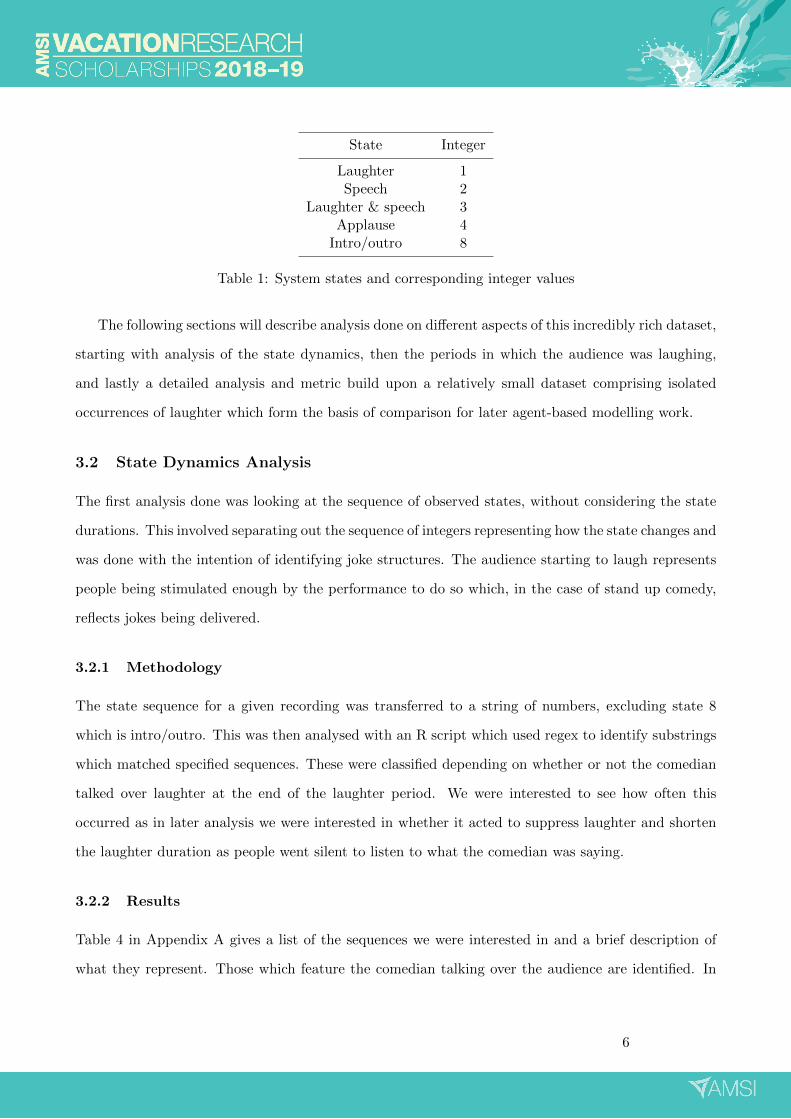
State Integer
Laughter 1Speech 2
Laughter & speech 3Applause 4
Intro/outro 8
Table 1: System states and corresponding integer values
The following sections will describe analysis done on different aspects of this incredibly rich dataset,
starting with analysis of the state dynamics, then the periods in which the audience was laughing,
and lastly a detailed analysis and metric build upon a relatively small dataset comprising isolated
occurrences of laughter which form the basis of comparison for later agent-based modelling work.
3.2 State Dynamics Analysis
The first analysis done was looking at the sequence of observed states, without considering the state
durations. This involved separating out the sequence of integers representing how the state changes and
was done with the intention of identifying joke structures. The audience starting to laugh represents
people being stimulated enough by the performance to do so which, in the case of stand up comedy,
reflects jokes being delivered.
3.2.1 Methodology
The state sequence for a given recording was transferred to a string of numbers, excluding state 8
which is intro/outro. This was then analysed with an R script which used regex to identify substrings
which matched specified sequences. These were classified depending on whether or not the comedian
talked over laughter at the end of the laughter period. We were interested to see how often this
occurred as in later analysis we were interested in whether it acted to suppress laughter and shorten
the laughter duration as people went silent to listen to what the comedian was saying.
3.2.2 Results
Table 4 in Appendix A gives a list of the sequences we were interested in and a brief description of
what they represent. Those which feature the comedian talking over the audience are identified. In
6
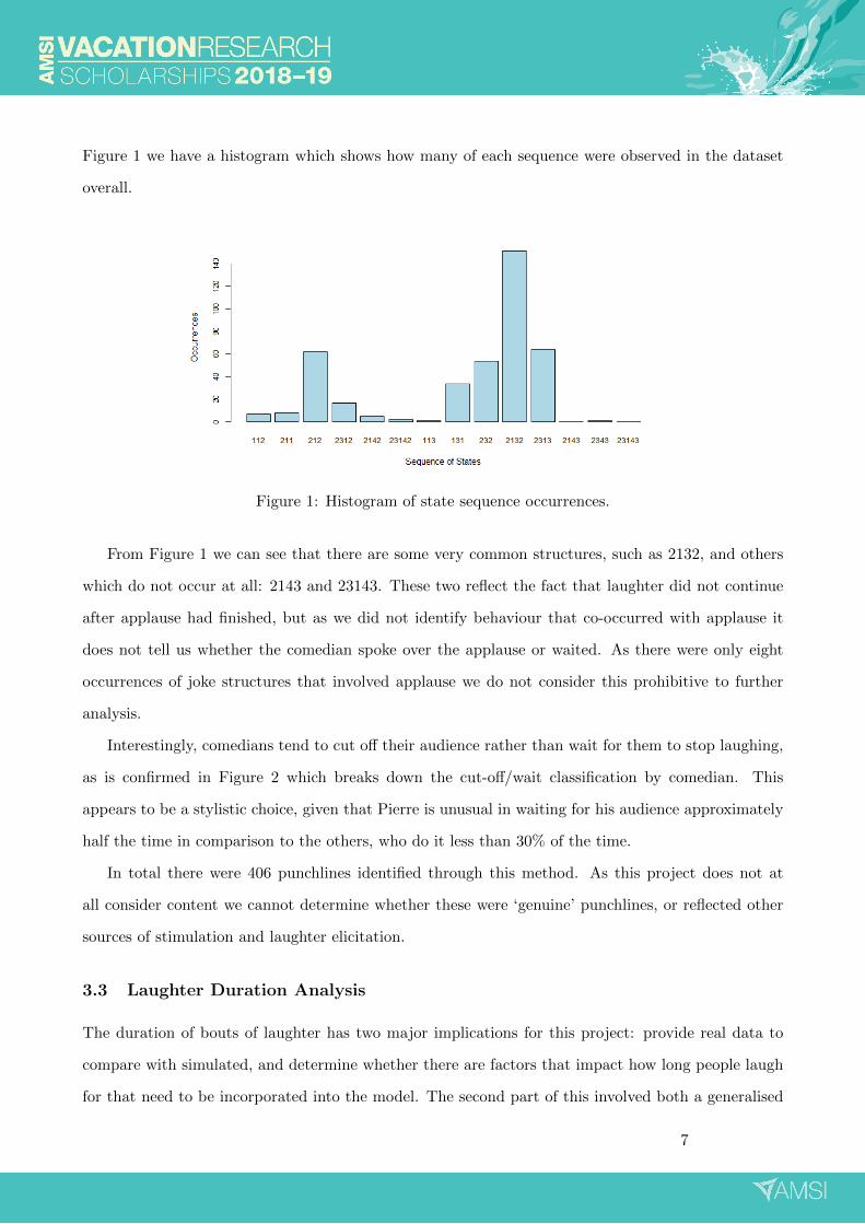
Figure 1 we have a histogram which shows how many of each sequence were observed in the dataset
overall.
Figure 1: Histogram of state sequence occurrences.
From Figure 1 we can see that there are some very common structures, such as 2132, and others
which do not occur at all: 2143 and 23143. These two reflect the fact that laughter did not continue
after applause had finished, but as we did not identify behaviour that co-occurred with applause it
does not tell us whether the comedian spoke over the applause or waited. As there were only eight
occurrences of joke structures that involved applause we do not consider this prohibitive to further
analysis.
Interestingly, comedians tend to cut off their audience rather than wait for them to stop laughing,
as is confirmed in Figure 2 which breaks down the cut-off/wait classification by comedian. This
appears to be a stylistic choice, given that Pierre is unusual in waiting for his audience approximately
half the time in comparison to the others, who do it less than 30% of the time.
In total there were 406 punchlines identified through this method. As this project does not at
all consider content we cannot determine whether these were ‘genuine’ punchlines, or reflected other
sources of stimulation and laughter elicitation.
3.3 Laughter Duration Analysis
The duration of bouts of laughter has two major implications for this project: provide real data to
compare with simulated, and determine whether there are factors that impact how long people laugh
for that need to be incorporated into the model. The second part of this involved both a generalised
7
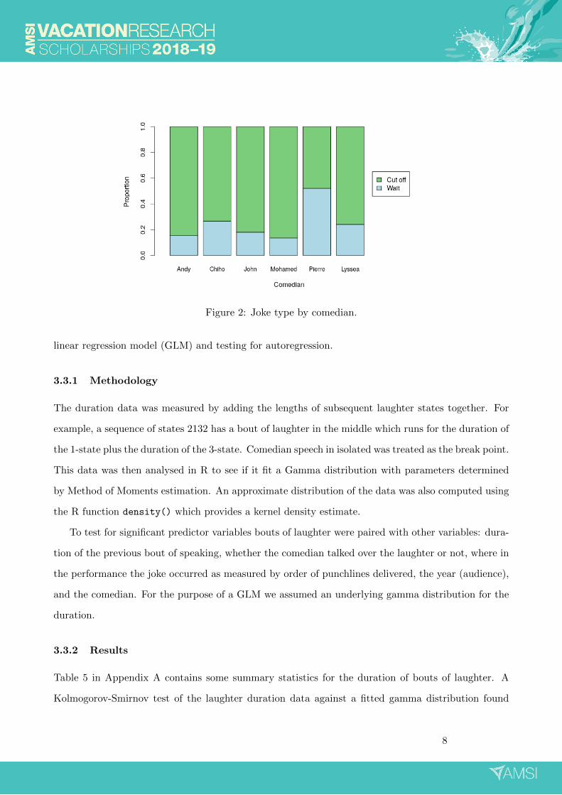
Figure 2: Joke type by comedian.
linear regression model (GLM) and testing for autoregression.
3.3.1 Methodology
The duration data was measured by adding the lengths of subsequent laughter states together. For
example, a sequence of states 2132 has a bout of laughter in the middle which runs for the duration of
the 1-state plus the duration of the 3-state. Comedian speech in isolated was treated as the break point.
This data was then analysed in R to see if it fit a Gamma distribution with parameters determined
by Method of Moments estimation. An approximate distribution of the data was also computed using
the R function density() which provides a kernel density estimate.
To test for significant predictor variables bouts of laughter were paired with other variables: dura-
tion of the previous bout of speaking, whether the comedian talked over the laughter or not, where in
the performance the joke occurred as measured by order of punchlines delivered, the year (audience),
and the comedian. For the purpose of a GLM we assumed an underlying gamma distribution for the
duration.
3.3.2 Results
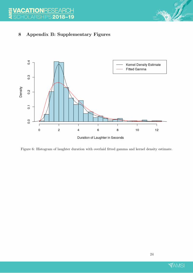
Table 5 in Appendix A contains some summary statistics for the duration of bouts of laughter. A
Kolmogorov-Smirnov test of the laughter duration data against a fitted gamma distribution found
8

a statistically significant difference (D = 0.10746, p-value = 0.0004467) at the α = 0.001 threshold,
which is strong evidence for this data not being gamma distributed. Furthermore, a histogram of the
data with overlaid fitted gamma (and kernel density) is Figure 6 in Appendix B, and clearly shows
that the kurtosis is higher for the observed data.
None of the predictor variables were statistically significant at the α = 0.05 threshold (see Table
6 in Appendix A for full output). In Figure 7 (Appendix B) we see that the residuals have somewhat
non-constant variance. Using back propagation we removed the predictor variables for comedian, year,
and how long the previous speech was as these were not statistically significant. Figure 8 (Appendix
B) shows the residual plot for the reduced GLM with only the order of punch line and whether
or not the comedian spoke over the laughter. This plot does not show non-constant variance. A
Shapiro-Wilk test for normality of residuals was statistically significant (W = 0.96849, p-value =
4.36 × 10⁻⁷) which is an issue, however given the underlying assumption of a gamma distribution it
is not surprising. Table 7 shows the GLM output, and that even these remaining predictor variables
were not statistically significant at α = 0.05. This result of non-significance is not necessarily rendered
invalid by the non-normality of the residuals, but should be treated with some caution.
A visual examination of autoregression plots for each of the 26 performances showed no overall
trend, or particular instance of significant autoregression in any single performance either.
This is not, however, bad news for our model as this indicates that the duration of laughter ie.
the audience behaviour, is independent of these factors. We must reiterate that we do not consider
content, and thus there are undoubtedly factors that do impact duration for all we cannot access
them. The core implication for the agent-based model is that we can deal with jokes independent of
one another. We may need to introduce some variation in laughter duration directly but we do not
have to deal with an entire performance.
3.4 Volume Analysis
We are interested in the proportion of the audience that is laughing for each of our performances.
However, just as we do not have access to individual behaviour directly, we are forced to use a proxy
metric. In this case we assume that different volumes of laughter represent different proportions of the
audience laughing. In particular, we assume that in isolated cases of mass laughter (which is audibly
different to a few individuals laughing), at the peak volume the entire audience is laughing. This
9
becomes our 100% point against which lower volumes are compared.
From this, we consider the time it takes to rise, and then fall, to particular quantile levels (0, 0.2,
0.4, 0.5, 0.6, 0.8, 1). These form the basis of a linearly interpolated 95% confidence region for the rise
and fall of audience laughter after an ‘average’ joke, which we can then compare to the behaviour of
our simulated audience.
3.4.1 Methodology
We first identified ‘exemplar’ laughter cases by first narrowing the dataset to those periods of laugher
which were not spoken over by the comedian or had applause following them. From that, we discarded
cases where only a few members of the audience laughed. This was done because our model is a first
attempt, and as such we are restricting to the case where a joke is good enough to get the entire
audience laughing. This left 46 MP3 files. The MP3 data was read into R as time series for the left
and right channels, which in terms of data is a wave function sampled at 44100Hz. We then took
the left channel, and the absolute value thereof, and decomposed it with an additive time series (see
Figure 9 for an example) of the form
Y (t) = T (t) + P (t) + e(t),
where Y (t) is the sampled amplitude, T (t) is a running mean trend, P (t) is the periodic behaviour4,
and e(t) is the random error. We use the trend as an approximate volume because this smooths out
the sound wave but retains the qualitative behaviour we want to consider. This was then normalised
to be proportional to the maximum from each sound clip, resulting in a proxy metric between 0 and
1 which represents the proportion of the audience that is laughing over time.
3.4.2 Results
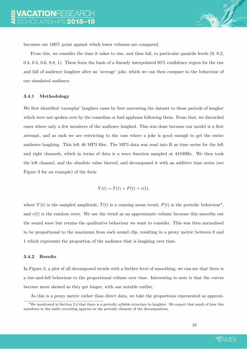
In Figure 3, a plot of all decomposed trends with a further level of smoothing, we can see that there is
a rise-and-fall behaviour to the proportional volume over time. Interesting to note is that the curves
become more skewed as they get longer, with one notable outlier.
As this is a proxy metric rather than direct data, we take the proportions represented as approxi-
4We mentioned in Section 2.4 that there is a periodic syllable structure to laughter. We expect that much of how thismanifests in the audio recording appears in the periodic element of the decomposition.
10
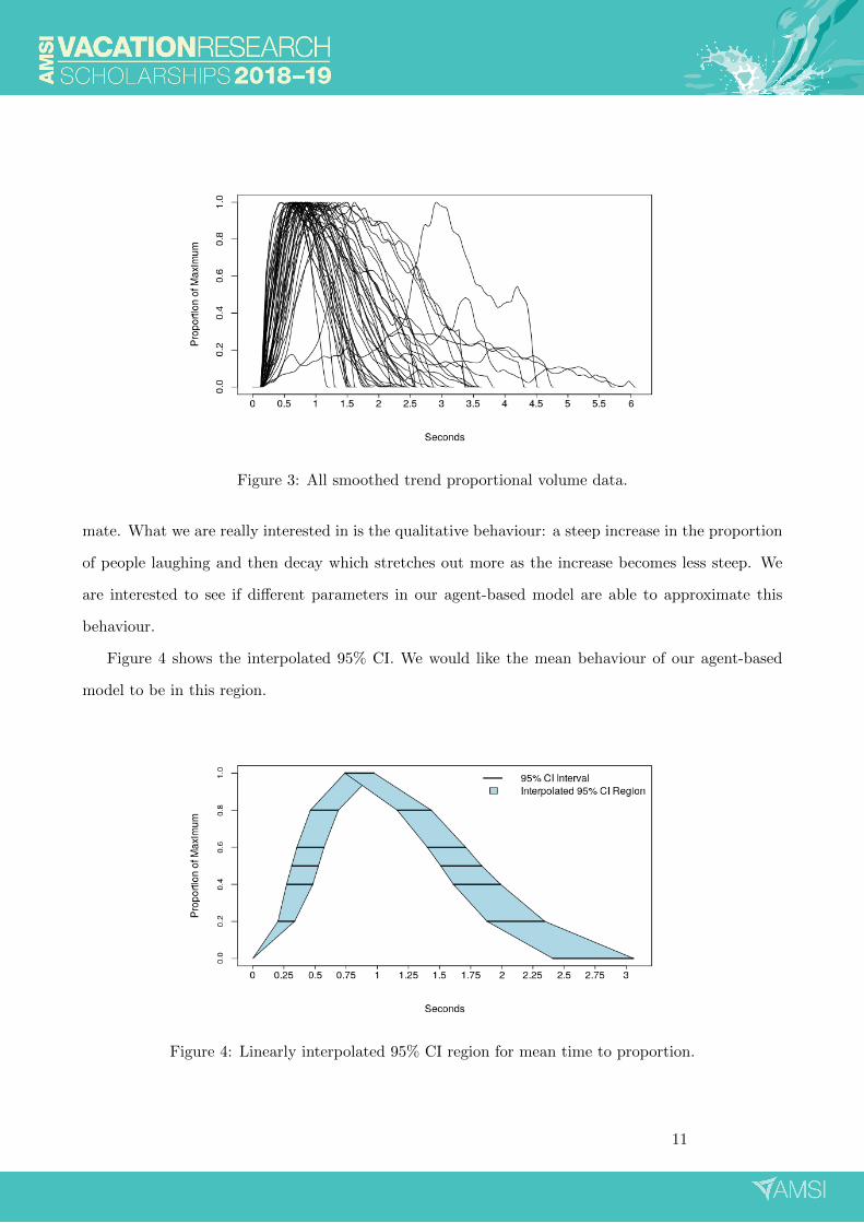
Figure 3: All smoothed trend proportional volume data.
mate. What we are really interested in is the qualitative behaviour: a steep increase in the proportion
of people laughing and then decay which stretches out more as the increase becomes less steep. We
are interested to see if different parameters in our agent-based model are able to approximate this
behaviour.
Figure 4 shows the interpolated 95% CI. We would like the mean behaviour of our agent-based
model to be in this region.
Figure 4: Linearly interpolated 95% CI region for mean time to proportion.
11

4 Agent-Based Model
We can now introduce the simulation model we have built to represent audience behaviour, and in
particular laughter propagation. This model is able to draw on both the social science background
described in Section 2 as well as the behaviour observed in our dataset from Section 3. First we
introduce agent-based modelling and the specific programming framework that the simulations are
done in, then we describe the model and some results.
4.1 Background of Agent-Based Modelling
An agent-based model represents a system of interest as a collection of autonomous agents, embedded
in an environment, and behaving according to a set of rules [Bonabeau, 2002]. It is a fundamentally
micro-level perspective in which system features emerge from the behaviour of the agents, and this is
advantageous for our model because we are interested in precisely the interaction between the agents,
and the individual behaviour of the agents themselves. Several researchers have shown that agent-
based models are particularly useful when dealing with complex human behaviour as it is able to
deal with non-linear, highly interactive, and changing rules [Gilbert and Terna, 2000] [Gilbert, 2004]
though one must be careful when describing the behaviour rules in order to adequately represent the
seemingly irrational tendencies that people often demonstrate [Bonabeau, 2002].
4.2 Environment - Rules - Agents
To represent agents seated in an audience we embed them in a complete graph, and assign them
coordinates as though they are seated at integer points in the plane in a grid. We then weight the
graph edges by the inverse squared Euclidean distance in order to represent the sound of laughter
propagating outwards.
Punchlines themselves are represented as an environmental impact that is the same for all agents
regardless of position. In order to reflect the stimulus and die out of a punchline we made use of a
skewed bump function, ψ : R→ R, with scaling parameter k ∈ R defined as
ψ(t) :=
exp
(−1
1−(
t−kk
)2 − t)
t ∈ (0, 2k),
0 otherwise.
(1)
12

The non-zero case has derivative with respect to t
∂ψ
∂t= exp
( −k2
2kt− t2− t)( 2k2(k − t)
t2(t− 2k)2− 1
),
which has a zero on (0, 2k) when
−t4 + 4kt3 − 4k2t2 − 2kt+ 2k3 = 0.
This allows us to numerically approximate the maximum for a given k, and then normalise the function
with respect to the maximum in order to control how much stimulation occurs at the peak. This is
something that may be changed when dealing with jokes of varying quality. We are however working
with the exemplar case and thus normalisation is reasonable.
The rules for agent behaviour are centred around an agent deciding whether they will start to
laugh in the next turn, then drawing from a gamma distribution for the duration of that laughter.
The decision is probabilistic, with the agent calculating a probability that they will start to laugh
based on the logistic function:
Pr(Agent j begins to laugh) =1
1 + exp(β0 + β1x1 +∑3
i=2 βixi,j), (2)
where the input variables are defined in Table 8 (Appendix A). The agent then randomly generates a
number from the uniform distribution on [0, 1], and if the generated number is less than the probability
that they start to laugh, they update their state to 1. It is important to note that this does not prevent
an agent starting a new bout of laughter before the last has finished. This is deliberate, as it is possible
to keep someone laughing for a long time with the repeated application of jokes.
The gamma distribution from which agents generate the duration of laughter is fitted to the
exemplar volume data in Section 3.4. Specifically the time between the curve first reaching 0.5, and
first dropping back down to 0.5. In this case the shape and scale parameters were 9.4732 and 0.13233
respectively.
Agents themselves have only a few properties. The first are coordinates for their location in the
audience, which go into the calculation of the graph weighting and animation output but otherwise
do not come into play. Second and perhaps most importantly is their laughter state, 0 or 1 for not
13

laughing and laughing. Third is the agent’s gigglability value which is sampled from the uniform
distribution on [−1, 1] when the agent is created and represents their overall propensity to laugh and
responsiveness to the material.
4.3 UODS Framework
We decided to use a ready-made Python framework for agent-based modelling in order to not spend
the entire project and then some trying to program one. As such, we adopted the Unified Opinion
Dynamics Simulator (UODS) system5 [Coates et al., 2018] and wrote specific modules for the initial
values, updater, and output as well as a configuration file for settings and parameter values. We
used algorithms provided as part of UODS for the graph generator (a complete graph in our case),
the group selector (complete), and no algorithm for the co-evolver as the structure of the graph was
unchanging.
The initial values module initialises agent parameters: starting laughter (0) and the individual
gigglability coefficient. It also assigns a weighting to the edges from the graph generator, and calculates
values for Equation 4.2 based on input punchline delivery times and scaling parameter.
The updater controls how agents determine their laughter state each turn. It implements Equation
4.2 based on input from the initialised joke function values and the current state of the rest of the
audience through the weighted graph.
Output from simulations consisted of a .csv file with the proportion of the audience laughing for
each time step and an optional animation. One simulation output one row of data. Animations may
be interesting for looking at propagation behaviour in the future, and there is a potential for more
detailed data to be simulated which outputs agent state along with location for points in time. With
this, it would be possible to calculate clustering effects however this is outside the scope of the current
project due to time constraints.
4.4 Simulation
The first task in bringing this simulation to fruition was determining the β coefficient values for
Equation 4.2. With no stimulation, humans are generally disinclined to laugh, though someone may
think of something amusing which acts as internal stimulation, rather than that derived from the
5Code base available at https://www.comses.net/codebases/46108c48-56b5-4999-b5a2-d7d3272fed03/releases/1.0.0/,with thanks to Adam Coates for his copious assistance.
14

performance. As such we set β0 to produce a baseline probability of laughing with no other effects
in play of 0.00001, and using the logit function this is determined to give β0 = −11.5129. Parameter
values for the other β coefficients were adapted over repeated simulations in order to get output that
displayed the increase-decay behaviour from Figure 4. We simply do not have the data to do any
better than this.
We assumed that at peak stimulation, with only the joke, there should be a 90% probability that
an agent starts to laugh. This gives a β1 value of 13.710, which was held constant for all of the
simulations. We then ran 10 simulations for values of β2 between 0 and 0.3, introducing the network
effect. Figure 10 in Appendix B shows the varying mean performance across these initial simulations6.
Note that β2 = 0 removes the network effect and represents just the joke bump function performance.
As we want the maximum to reach 100%, but we also want a rounded rather than square curve. As
such, we try β2 = 0.1 and β2 = 0.15 for further simulation.
The next step is to incorporate the gigglability coefficient. This serves to add variation to agent
behaviour. Figure 5 shows the full model against an interpolated CI region from a subset of Section
3.4 data7. This subset was from sound clips with less than 2 seconds of duration, chosen because the
duration of the laughter observed in the simulation was less than 2 seconds long. This is reasonable
because we have not introduced variance in the mean duration for laughter. In order to match the
audible start of laughter, the simulated data was translated to be zeroed at the start of agents laughing.
What is noticable in Figure 5 is that the curves for both β2 parameters are considerably more square
than the confidence region. However, the peak of the confidence region corresponds to approximately
the centre of the simulated curves. This suggests that the model is reasonable for duration although
it is not clear how that should relate to the parameters used for the gamma distribution from which
agents drew their laughter duration.
5 Discussion
This project is limited by data availability. As it is a data-motivated construction the lack of individual
level detail in datasets limits both how well the model can be built in terms of the behaviour rules
that agents obey, and how well it can be checked against the real world data. The proxy volume
6Simulations were done with an audience of 500, because an audience of 3000 which matches the MICFG made eachsimulation take two to three hours.
7See Figure 11 in Appendix B for a comparison with the full dataset CI
15

Figure 5: Mean proportion for different β2 values in full model.
metric in particular is not ideal, as it is subject to inaccuracies around change in each individual’s
volume output as they laugh as well as interference from the comedian’s performance speaking over
the top which seriously restricted the sample size. None the less, we think that the agent-based model
is an interesting first effort that succeeds in representing some features observed in the data, namely
the build up and decay of people laughing after a punch line has been delivered. It successfully
incorporates a network although we are not able to assess the realism of our chosen weighting between
the network and the joke stimulus.
This project has considerable scope for ongoing work. The most obvious is the procurement of
a better dataset. With facial recognition technology it is potentially possible to identify individuals
laughing in an audience automatically [Petridis et al., 2013] which could provide a much richer source
of information. There is also scope to introduce a machine learning algorithm to classify more MP3
recordings, as massed laughter as a wave form is similar to white noise even though individual laughter
looks more like speech [Bickley and Hunnicutt, 1992].
Within the agent-based model itself we have explored very little of the parameter space. In
particular we have not investigated the impact of the laughter duration distribution. Changing the
gamma mean, or indeed the distribution family, may have interesting effects on agent behaviour.
Additional computing power would enable us to expand the size of the audience to better reflect
16
the nearly 3000 who attend the MICFG event, which would make it more appropriate to directly
compare simulation to the current dataset. We also need to better consider the spacing and location
of the audience as integer points in a plane which then are used as a source of network weighting may
introduce problems in comparison to a more tightly packed real audience, or a real audience with a
different distribution in space.
6 Conclusions
This project has produced an interesting dataset for a comedy performance system, incorporating both
the comedian and audience behaviours. The agent-based model developed out of this and ideas from
social science research has been a reasonable start for further work in examining laughter propagation
as well as the impact of planted agents on the audience experience. With considerable scope for further
development we believe that there is more insight and information yet to come.
17
References
[Bickley and Hunnicutt, 1992] Bickley, C. A. and Hunnicutt, S. (1992). Acoustic analysis of laughter.
In Second International Conference on Spoken Language Processing.
[Bonabeau, 2002] Bonabeau, E. (2002). Agent-based modeling: Methods and techniques for simulat-
ing human systems. Proceedings of the National Academy of Sciences, 99(suppl 3):7280–7287.
[Brock, 2017] Brock, A. (2017). Modelling the complexity of humour–insights from linguistics. Lingua,
197:5–15.
[Coates et al., 2018] Coates, A., Han, L., and Kleerekoper, A. (2018). A unified framework for opinion
dynamics. In Proceedings of the 17th International Conference on Autonomous Agents and Multia-
gent Systems, pages 1079–1086. International Foundation for Autonomous Agents and Multiagent
Systems.
[Davis, 2008] Davis, D. (2008). Communication and humor. The Primer of Humour Research, Berlin
and New York: Mouton de Gruyter, pages 543–568.
[Gilbert, 2004] Gilbert, N. (2004). Agent-based social simulation: dealing with complexity. The
Complex Systems Network of Excellence, 9(25):1–14.
[Gilbert and Terna, 2000] Gilbert, N. and Terna, P. (2000). How to build and use agent-based models
in social science. Mind & Society, 1(1):57–72.
[Kuipers, 2008] Kuipers, G. (2008). The sociology of humor. The primer of humor research, pages
361–398.
[Lymperopoulos and Ioannou, 2015] Lymperopoulos, I. N. and Ioannou, G. D. (2015). Online social
contagion modeling through the dynamics of integrate-and-fire neurons. Information Sciences,
320:26–61.
[Petridis et al., 2013] Petridis, S., Martinez, B., and Pantic, M. (2013). The mahnob laughter
database. Image and Vision Computing, 31(2):186–202.
[Provine, 1992] Provine, R. R. (1992). Contagious laughter: Laughter is a sufficient stimulus for laughs
and smiles. Bulletin of the Psychonomic Society, 30(1):1–4.
18

[Ritchie, 1999] Ritchie, G. (1999). Developing the incongruity-resolution theory. Technical report.
[Ruch, 2008] Ruch, W. (2008). Psychology of humor. The primer of humor research, page 17.
19
7 Appendix A: Supplementary Tables
Bit Behaviour
1st Audience laughter2nd Comedian speech3rd Audience applause4th Intro/Outro
Table 2: Bit indicator and corresponding behaviour.
Comedian Samples Years
Andy 4 ’13, ’15, ’16, ’17Chiho 4 ’14, ’16, ’17John 4 ‘14, ’15, ’16, ’17
Mohammed 5 ’13, ’14, ’15, ’16, ’17Pierre 4 ’13, ’14, ’15, ’17Lyssea 5 ’13, ’14, ’15, ’16, ’17
Table 3: MP3 sample information.
Sequence Description Sequence Description
112 The second of two bouts of
laughter without speech in be-
tween, associated with the co-
median doing some form of
amusing motion.
131 Comedian talking over laugh-
ter which continues after they
stop speaking.
211 The first of two bouts of
laughter, which starts after a
comedian stops talking.
232 Laughter occurring over the
top of continuing speech
212 Comedian speaks, stops
speaking and laughter occurs,
then laughter stops and
speech starts again.
2132 Comedian delivers joke after
which the audience laughs,
but the comedian talks over
the top of the laughter before
it dies out.
20
2312 Audience starts to laugh be-
fore comedian has finished
talking, but the comedian
waits for the audience to fin-
ish laughing.
2313 Audience starts to laugh be-
fore the comedian has finished
and then the comedian talks
over the laughter.
2142 Laughter begins after come-
dian has stopped speaking
and applause breaks out as
well. Audience stops applaud-
ing and then the comedian
speaks again.
2143 Audience laughs after co-
median has stopped talking
and applauds, but continues
laughing past applause over
which the comedian speaks.
23142 Audience starts to laugh be-
fore comedian has finished
speaking, then applauds af-
ter a period of laughter alone.
Comedian does not speak over
laughter at the end.
2343 Audience starts to laugh be-
fore the comedian has finished
speaking and applauds the co-
median. Laughter at the end
of the applause is spoken over
113 The second of two bouts of
laughter after some form of
physical stimulus, with the
comedian talking over the
laughter.
23143 Laughter starts before come-
dian stops talking, laughter
continues and then applause
begins. After applause is done
laughter continues over which
the comedian speaks.
Table 4: Punchline delivery in terms of dynamic behaviour.
21

Statistic Sample Estimate
Mean 2.988431
Variance 3.241026
Skewness 1.969909
Kurtosis 5.08567
Table 5: Summary statistics of laughter duration.
Coefficients Estimate Std. Error t-value Pr(> |t|)
Intercept 0.3903069 0.0421776 9.254 < 2e− 16
laughCutoffWait -0.0204147 0.0241242 -0.846 0.3980
laughterOrder -0.0040579 0.0023219 -1.748 0.0814
laughterPrecSpeech -0.0005523 0.0013590 -0.406 0.6847
laughterYear2014 0.0113551 0.0361095 0.314 0.7534
laughterYear2015 0.0420187 0.0353578 1.188 0.2355
laughterYear2016 -0.0335557 0.0333630 -1.006 0.3152
laughterYear2017 0.0006009 0.0325146 0.018 0.9853
laughterComChiho -0.0163541 0.0377409 -0.433 0.6650
laughterComJohn 0.0618504 0.0447321 1.383 0.1676
laughterComLyssea -0.0340647 0.0348207 -0.978 0.3286
laughterComMohammed -0.0232578 0.0354869 -0.655 0.5126
laughterComPierre -0.0394973 0.0377170 -1.047 0.2957
Table 6: GLM output for laughter duration.
Coefficients Estimate Std. Error t-value Pr(> |t|)
Intercept 0.378364 0.022653 16.702 < 2e− 16
laughterOrder -0.004498 0.002353 -1.911 0.0568
laughCutoffWait -0.031573 0.023433 -1.347 0.1787
Table 7: Reduced GLM output for laughter duration.
22

Parameter Description
x1 Punchline function output,
x2,j Weighted sum of indicator variables for otheragents laughter calculated as
∑pk=1wk,jIk where
wk,j is the inverse squared Euclidean distance,
x3,j Agent gigglability value.
Table 8: Input terms for logistic function
23
8 Appendix B: Supplementary Figures
Figure 6: Histogram of laughter duration with overlaid fitted gamma and kernel density estimate.
24

Figure 7: Residual plot for GLM.
Figure 8: Residual plot for reduced GLM.
25

Figure 9: Example decomposition of time series.
Figure 10: Mean proportion for different β2 values.
26
Figure 11: Mean proportion for different β2 values in full model against full CI region.
27
Related Documents