A geometric mass-preserving redistancing scheme for the ...

A geometric mass-preserving redistancing scheme forthe level set function

Roberto F. Ausasa, Enzo A. Daria, Gustavo C. Buscagliab

aCentro Atomico Bariloche e Instituto Balseiro, 8400, Bariloche, Argentina,

[email protected], [email protected] de Ciencias Matematicas e de Computacao, Univ. de Sao Paulo, Sao Carlos, Brasil,

e-mail: [email protected]

July 7, 2009

Keywords: Level Set Method, Reinitialization, Redistancing, Curvilinear Coordi-nates.

Abstract.In this paper we describe and evaluate a geometric mass-preserving redistancing procedure

for the level set function on general structured grids. The proposed algorithm is adapted from

a recent finite-element-based method and preserves the mass by means of a localized mass cor-

rection. A salient feature of the scheme is the absence of adjustable parameters. The algorithm

is tested in two and three spatial dimensions and compared with the widely used PDE-based

redistancing method using structured Cartesian grids. Through the use of quantitative error

measures of interest in level set methods, we show that the overall performance of the proposed

geometric procedure is better than PDE-based reinitialization schemes, since it is more robust

with comparable accuracy. We also show that the algorithm is well–suited for the highly–streched

curvilinear grids used in CFD simulations.

1 Introduction

The level set method, introduced by Sethian and Osher in 1988 [1], has been exten-sively used in the past few years to treat problems involving free surfaces, basically dueto its simplicity to deal with the complex topological changes that interfaces might un-dergo along their transport in a general situation. Additionally, quantities such as thecurvature of the interface and other related information can be extracted from the levelset function making it a very attractive and powerful tool for problems in two and threespatial dimensions.

As is well known, one of the main drawbacks of this method for free surface problemsinvolving incompressible flows is the lack of mass conservation and excessive diffusion,which leads to unphysical motions of the interface that severely deteriorate the accuracyand stability of the results. These difficulties have been addressed in basically threedifferent ways:

• by improving the numerical algorithms used to transport the level set function;

• by combining the level set method with other computational techniques;

• by trying to keep the level set function as regular as possible, using the so calledreinitialization or redistancing procedures.

Regarding the first alternative, there are many methods to solve the level set equa-tion, such as finite volume and finite difference methods which combine total variationdiminishing (TVD) schemes in time, introduced by Shu and Osher [2, 3], and essentiallynon-oscillatory (ENO) schemes in space, based on the ideas firstly proposed by Hartenand coworkers [4, 5] to solve Hamilton-Jacobi type equations. In this area, the TVD-Runge-Kutta and Hamilton-Jacobi Weighted-ENO scheme developed in [6] is consideredto be state-of-the-art for solving the level set equation within the framework of eulerianmethods [7]. In this case, curvilinear coordinates can be used to deal with complex ge-ometries (see for instance [8] and [9]). It should be mentioned that TVD schemes can alsobe used in space as flux limiter methods, as done for instance by Olsson and Kreiss [10].Stabilized finite elements and discontinuous Galerkin methods are used as well for treatingthe level set equation. In this case, unstructured meshes can be employed and local gridrefinement becomes an easy task. A comparison of such methods is done in [11]. In [12]a discontinuous Galerkin method is proposed and compared with several other methodsincluding the ENO/RK(3) scheme presented in [13] and the HJ-WENO(5)/RK(3) schemeused in [14, 15]. Finally, semi-Lagrangian schemes, which can be implemented in verysimple and efficient ways, are also used in level set methods (see [16, 17, 14]).

With respect to the second alternative in the bulleted list above, hybrid methods thatcombine the level set method either with Lagrangian particles or with the VOF (volume offluid) method have been developed. The first option consists in moving massless particlesforward in time in order to redefine the level set function by means of some procedure atthe end of each time step or with a predefined frequency. See for instance [14, 15] and[18]. The other option uses the VOF method (see e.g. [19]), another surface capturingmethod for free surface flows, to correct the level set function so as to locally enforce massconservation as done by Sussman in [20] and [21] for example.

In this article we focus on the redistancing procedure. Its purpose is to ensure that thelevel set function remains smooth close to the interface. This is achieved by periodically

2

redefining it, while trying to maintain the interface intact. The reinitialization improvesthe robustness of the computations by keeping the distortion of the level set function undercontrol. A natural choice to reinitialize the level set function is the signed distance functionto the interface. The idea of reinitialization was first presented in the work of Chopp [22].Later, Tsitsiklis [23] proposed in a completely different framework, a method that can beused for the construction of distance functions, and therefore for reinitialization, knownas the fast marching method, further popularized by Sethian (see [24] and [25]). A secondpaper of Chopp [26], that introduces some improvements to the method, can also bementioned in this context. It should be pointed out that reinitialization can be avoidedusing a velocity extension that preserves the signed distance function (see [27] and [28]).On the other hand, several PDE-based methods have been devised for the purpose ofredistancing, which solve the so-called reinitialization equation as originally proposed bySussman and coworkers [29, 30, 13].

It should be pointed out that, in general, it is not possible to reinitialize the level setfunction maintaining the interface intact in a discrete problem. In fact, the space of levelset functions that share the same given interface is extremely small [31] and it is likelythat none of its elements provides a reasonable approximation to the distance function.The consequence of this is that each reinitialization distorts the interface to some extent,implying a local numerical creation/destruction of fluid mass. However, this distortion isnot explicit in PDE-based methods but embedded in the discretization adopted for thereinitialization equation. The use of high-order schemes, together with ad-hoc correctionterms, are needed to minimize the interface distortion during reinitialization, which other-wise completely destroys the accuracy of the computations [7]. Though improved versionsof PDE-based reinitialization exist for Cartesian grids (see e.g. [32] and [33]), they arenot well–suited for highly–streched curvilinear grids.

In this article we adapt the reinitialization scheme of Mut et al [34] to the case ofstructured, curvilinear finite difference grids. The scheme was originally developed forunstructured meshes of linear finite elements, and a simple subdivision of each quadri-lateral (or of each hexahedron in 3D) is used to build a mesh suitable for applying it.The advantages of the proposed reinitialization scheme are its simplicity, its flexibility tohandle arbitrarily distorted meshes, and the absence of adjustable parameters.

We begin by showing the necessity of redistancing in Section 2. In Section 3 wedescribe the proposed method, together with the TVD Runge-Kutta third-order ENOscheme that is used to evolve the level set equation, for which we use a finite volumeimplementation very similar to that presented in [8]. Since the proposed method is basedon a piecewise-linear representation of the level set function, concerns may arise as to itsaccuracy. Section 3 also contains a brief summary of a widely used PDE-based method,the HJWENO-RK scheme of Peng et al [6]. This method will be compared to the proposedone in the numerical examples.

In section 4, numerical experiments are shown in two and three spatial dimensions,including the rigid rotation of Zalesak’s disk, the deformation of a circle under a swirlingflow vortex, and the deformation of a 3D sphere, which are classical benchmark cases inlevel set methods. Specific measures of error of interest in free surface problems are usedto evaluate the results. Finally, to illustrate the versatility of the proposed geometricredistancing scheme, we couple it with a finite difference upwind method in curvilinearcoordinates that uses a second order TVD van Albada scheme as flux limiter for thetransport of the level set function, similar to the one used in CFDShip-Iowa [9]. We

3

present numerical examples using curvilinear grids that have appreciable distortion inorder to be able to test the mass-preserving scheme in relevant situations that mightappear in real CFD computations. We draw some conclusions in section 6.

2 Motivation

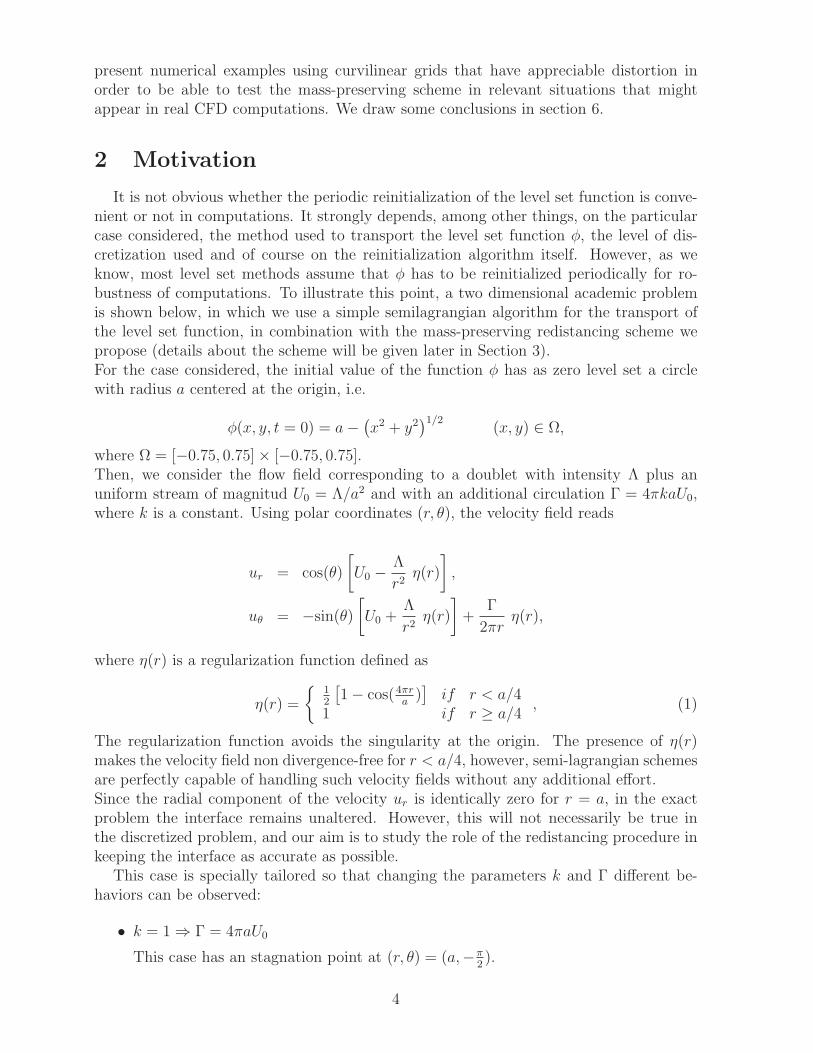
It is not obvious whether the periodic reinitialization of the level set function is conve-nient or not in computations. It strongly depends, among other things, on the particularcase considered, the method used to transport the level set function φ, the level of dis-cretization used and of course on the reinitialization algorithm itself. However, as weknow, most level set methods assume that φ has to be reinitialized periodically for ro-bustness of computations. To illustrate this point, a two dimensional academic problemis shown below, in which we use a simple semilagrangian algorithm for the transport ofthe level set function, in combination with the mass-preserving redistancing scheme wepropose (details about the scheme will be given later in Section 3).For the case considered, the initial value of the function φ has as zero level set a circlewith radius a centered at the origin, i.e.

φ(x, y, t = 0) = a−(

x2 + y2)1/2

(x, y) ∈ Ω,

where Ω = [−0.75, 0.75]× [−0.75, 0.75].Then, we consider the flow field corresponding to a doublet with intensity Λ plus anuniform stream of magnitud U0 = Λ/a2 and with an additional circulation Γ = 4πkaU0,where k is a constant. Using polar coordinates (r, θ), the velocity field reads

ur = cos(θ)

[

U0 −Λ

r2η(r)

]

,

uθ = −sin(θ)

[

U0 +Λ

r2η(r)

]

+Γ

2πrη(r),

where η(r) is a regularization function defined as

η(r) =

12

[

1− cos(4πra

)]

if r < a/41 if r ≥ a/4

, (1)

The regularization function avoids the singularity at the origin. The presence of η(r)makes the velocity field non divergence-free for r < a/4, however, semi-lagrangian schemesare perfectly capable of handling such velocity fields without any additional effort.Since the radial component of the velocity ur is identically zero for r = a, in the exactproblem the interface remains unaltered. However, this will not necessarily be true inthe discretized problem, and our aim is to study the role of the redistancing procedure inkeeping the interface as accurate as possible.

This case is specially tailored so that changing the parameters k and Γ different be-haviors can be observed:

• k = 1⇒ Γ = 4πaU0

This case has an stagnation point at (r, θ) = (a,−π2).

4

• k > 1⇒ Γ > 4πaU0

In this case the stagnation point occurs at some point (r, θ) = (r1,−π2), r1 > a.

The cases corresponding to k < 1, with to two stagnation points at (r, θ) = (a,−π2− θs)

and (r, θ) = (a,−π2

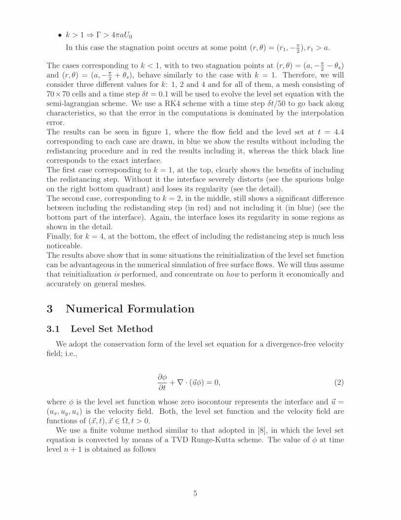
+ θs), behave similarly to the case with k = 1. Therefore, we willconsider three different values for k: 1, 2 and 4 and for all of them, a mesh consisting of70×70 cells and a time step δt = 0.1 will be used to evolve the level set equation with thesemi-lagrangian scheme. We use a RK4 scheme with a time step δt/50 to go back alongcharacteristics, so that the error in the computations is dominated by the interpolationerror.The results can be seen in figure 1, where the flow field and the level set at t = 4.4corresponding to each case are drawn, in blue we show the results without including theredistancing procedure and in red the results including it, whereas the thick black linecorresponds to the exact interface.The first case corresponding to k = 1, at the top, clearly shows the benefits of includingthe redistancing step. Without it the interface severely distorts (see the spurious bulgeon the right bottom quadrant) and loses its regularity (see the detail).The second case, corresponding to k = 2, in the middle, still shows a significant differencebetween including the redistanding step (in red) and not including it (in blue) (see thebottom part of the interface). Again, the interface loses its regularity in some regions asshown in the detail.Finally, for k = 4, at the bottom, the effect of including the redistancing step is much lessnoticeable.The results above show that in some situations the reinitialization of the level set functioncan be advantageous in the numerical simulation of free surface flows. We will thus assumethat reinitialization is performed, and concentrate on how to perform it economically andaccurately on general meshes.

3 Numerical Formulation

3.1 Level Set Method

We adopt the conservation form of the level set equation for a divergence-free velocityfield; i.e.,

∂φ

∂t+∇ · (~uφ) = 0, (2)

where φ is the level set function whose zero isocontour represents the interface and ~u =(ux, uy, uz) is the velocity field. Both, the level set function and the velocity field arefunctions of (~x, t), ~x ∈ Ω, t > 0.

We use a finite volume method similar to that adopted in [8], in which the level setequation is convected by means of a TVD Runge-Kutta scheme. The value of φ at timelevel n+ 1 is obtained as follows

5

−0.2

−0.1

0

0.1

0.2

−0.2 −0.1 0 0.1 0.2

−0.22

−0.18

−0.14

−0.1

−0.22 −0.18 −0.14 −0.1

−0.2

−0.1

0

0.1

0.2

−0.2 −0.1 0 0.1 0.2

0.11

0.13

0.15

0.17

0.11 0.13 0.15 0.17

−0.2

−0.1

0

0.1

0.2

−0.2 −0.1 0 0.1 0.2

Γ = 4πaU0

Γ = 8πaU0

Γ = 16πaU0

Without Redistancing

Initial Condition

With Redistancing

Figure 1: Flow fields and level sets after several time steps for all the cases considered.Top: k = 1, Middle: k = 2, Bottom: k = 4. The thick black line corresponds to the exactinterface, the thin blue line to the transport without the redistancing step and the thinred line corresponds to the transport including the redistancing procedure at the end ofeach time step.

6

φ(1) = φn − δt L(φn, tn),

φ(2) =3

4φn +

1

4φ(1) −

1

4δt L(φ(1), tn + δt), (3)

φn+1 =1

3φn +

2

3φ(2) −

2

3δt L(φ(2), tn +

1

2δt),

where φn is the value of φ at the time level n, δt is the time step and L(φ, t) is the spatialoperator in equation (2), i.e.

L(φ, t) = ∇ · (~uφ). (4)

Now, in order to obtain a fully discrete method, that for the sake of simplicity is presentedhere in two spatial dimensions, we subdivide the computational domain Ω = [0, Lx]×[0, Ly]into I and J uniform cells in the x and y directions respectively, such that the grid spacingwill be given by δx and δy. Then, the discrete form of (4) for the control volume (i, j)will be simply given by

L(φ) =(uxφ)i+1/2,j − (uxφ)i−1/2,j

δx+

(uyφ)i,j+1/2 − (uyφ)i,j−1/2

δy. (5)

The extension to three spatial dimensions is straightforward. In this scheme, ux and uy

are computed at the cell faces, but φ is given at the cell centre of the control volume,from which, the cell face values of φ (φi+1/2,j, φi,j+1/2, ...) are built by using a third-orderaccurate ENO interpolation. Details for the construction of the corresponding stencilscan be found in [3] or [8].

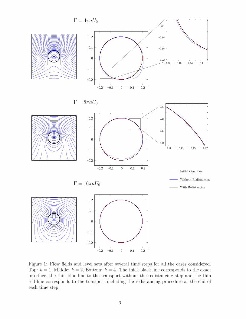
3.2 Geometric mass-preserving redistancing scheme

The geometric mass-preserving reinitialization algorithm proposed here was originallydevised to be used within the finite element framework [34], in which the level set functionis linearly interpolated over each simplex of an arbitrary triangulation Th (triangles in 2Dand tetrahedra in 3D).

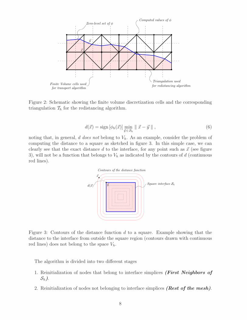
To adapt it to finite volume structured meshes we thus define a finite element partitionTh of Ω and assign the values of φ, computed at the center of gravity of the finite volumecells, as nodal values on Th. In 2D, the triangulation Th is obtained by dividing each cellinto two triangles as shown in Figure 2, whereas in 3D each hexahedral cell is dividedinto six tetrahedra. Therefore, the number of simplices in this partition will be two(respectively, six) times the number of cells used for the finite volume discretization inthe 2D (respectively, 3D) case. The way this subdivision is made does not really influencethe performance of the redistancing scheme.

We now proceed to describe the geometric redistancing algorithm. Let Vh be the spaceof continuous functions that are linear inside each simplex of Th. Let φh ∈ Vh be afunction, and let Sh be its zero-level set. Our aim is to find a function φh ∈ Vh whichapproximates the signed distance function d to Sh defined by

7

Triangulation used

for redistancing algorithmFinite Volume cells usedfor transport algorithm

Computed values of φZero-level set of φ

~y

~x

Figure 2: Schematic showing the finite volume discretization cells and the correspondingtriangulation Th for the redistancing algorithm.

d(~x) = sign [φh(~x)] min~y ∈Sh

‖ ~x− ~y ‖ , (6)

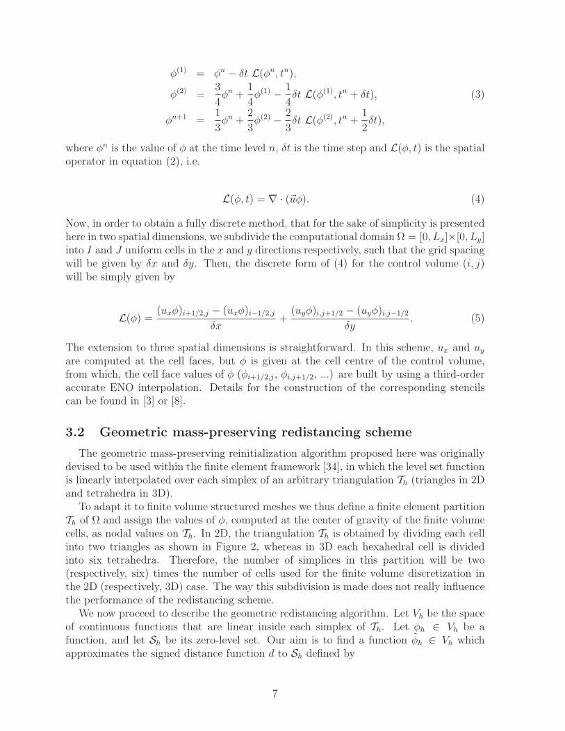
noting that, in general, d does not belong to Vh. As an example, consider the problem ofcomputing the distance to a square as sketched in figure 3. In this simple case, we canclearly see that the exact distance d to the interface, for any point such as ~x (see figure3), will not be a function that belongs to Vh as indicated by the contours of d (continuousred lines).

~y Square interface Shd(~x)

~x

Contours of the distance function

Figure 3: Contours of the distance function d to a square. Example showing that thedistance to the interface from outside the square region (contours drawn with continuousred lines) does not belong to the space Vh.

The algorithm is divided into two different stages

1. Reinitialization of nodes that belong to interface simplices (First Neighbors ofSh).

2. Reinitialization of nodes not belonging to interface simplices (Rest of the mesh).

8

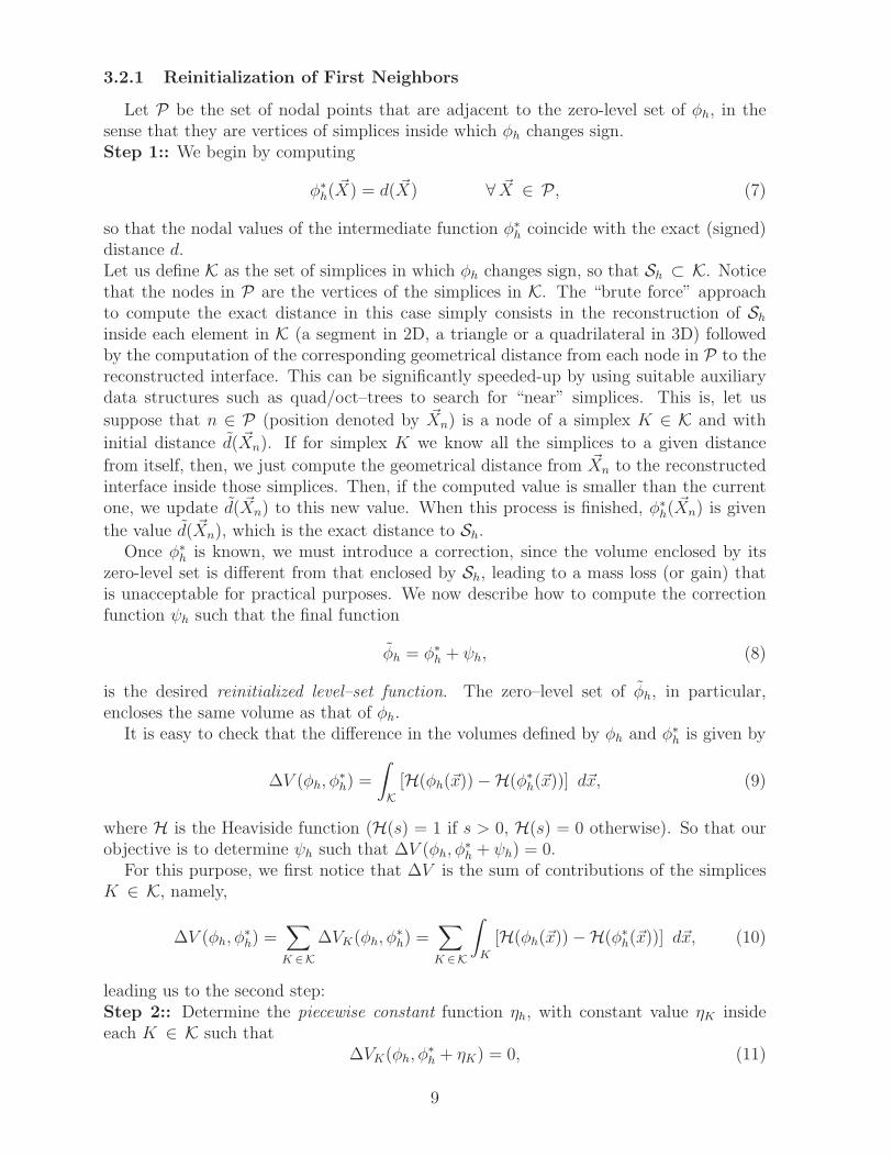
3.2.1 Reinitialization of First Neighbors

Let P be the set of nodal points that are adjacent to the zero-level set of φh, in thesense that they are vertices of simplices inside which φh changes sign.Step 1:: We begin by computing

φ∗

h( ~X) = d( ~X) ∀ ~X ∈ P, (7)

so that the nodal values of the intermediate function φ∗h coincide with the exact (signed)

distance d.Let us define K as the set of simplices in which φh changes sign, so that Sh ⊂ K. Noticethat the nodes in P are the vertices of the simplices in K. The “brute force” approachto compute the exact distance in this case simply consists in the reconstruction of Sh

inside each element in K (a segment in 2D, a triangle or a quadrilateral in 3D) followedby the computation of the corresponding geometrical distance from each node in P to thereconstructed interface. This can be significantly speeded-up by using suitable auxiliarydata structures such as quad/oct–trees to search for “near” simplices. This is, let us

suppose that n ∈ P (position denoted by ~Xn) is a node of a simplex K ∈ K and with

initial distance d( ~Xn). If for simplex K we know all the simplices to a given distance

from itself, then, we just compute the geometrical distance from ~Xn to the reconstructedinterface inside those simplices. Then, if the computed value is smaller than the currentone, we update d( ~Xn) to this new value. When this process is finished, φ∗

h(~Xn) is given

the value d( ~Xn), which is the exact distance to Sh.Once φ∗

h is known, we must introduce a correction, since the volume enclosed by itszero-level set is different from that enclosed by Sh, leading to a mass loss (or gain) thatis unacceptable for practical purposes. We now describe how to compute the correctionfunction ψh such that the final function

φh = φ∗

h + ψh, (8)

is the desired reinitialized level–set function. The zero–level set of φh, in particular,encloses the same volume as that of φh.

It is easy to check that the difference in the volumes defined by φh and φ∗h is given by

∆V (φh, φ∗

h) =

∫

K

[H(φh(~x))−H(φ∗

h(~x))] d~x, (9)

where H is the Heaviside function (H(s) = 1 if s > 0, H(s) = 0 otherwise). So that ourobjective is to determine ψh such that ∆V (φh, φ

∗h + ψh) = 0.

For this purpose, we first notice that ∆V is the sum of contributions of the simplicesK ∈ K, namely,

∆V (φh, φ∗

h) =∑

K ∈K

∆VK(φh, φ∗

h) =∑

K ∈K

∫

K

[H(φh(~x))−H(φ∗

h(~x))] d~x, (10)

leading us to the second step:Step 2:: Determine the piecewise constant function ηh, with constant value ηK insideeach K ∈ K such that

∆VK(φh, φ∗

h + ηK) = 0, (11)

9

Notice that Eq. 11 is a nonlinear equation for ηK , which is solved independently for eachK using a simple Regula Falsi procedure that converges in very few iterations.

The piecewise-constant function ηh computed in this way contains the information ofhow much volume loss or gain is contributed by each simplex in K. It is not possible,however, to define φh as φ∗

h+ηh, because ηh is a discontinuous function and is thus multiplyvalued at the nodes in P .Step 3:: We now compute a continuous function ξh as an approximate L2-orthogonalprojection of ηh onto the space of piecewise continuous functions inK. This is implementedin practice by simply computing the nodal values of ξh averaging over the simplices thatshare a node. Let I be a node in P , and let NI be the number of simplices in K thatcontain I, then we define

ξh( ~XI) =1

NI

∑

K ∈ KI ∈ K

ηK . (12)

Step 4:: Finally, the correction ψh is computed on P as

ψh = C ξh, (13)

where C is the constant that globally preserves volume; i.e., C satisfies

∆V (φh, φ∗

h + Cξh) = 0. (14)

This nonlinear equation for C is again solved by a simple Regula Falsi method and con-verges in very few iterations. From the description above it is evident that there are noadjustable parameters in the scheme, except for the numerical tolerance in the RegulaFalsi algorithms, which does not play any significant role since convergence to machineprecision takes place quickly. Steps 1,2,3 and 4 are summarized in Table 1.

The main advantage of the algorithm, as compared to previous ones, is that ξh local-izes the correction in those regions where the mass loss/gain produced by φ∗

h is largest;correcting φ∗

h by a constant, as done by other authors [35], corresponds to taking ξh = 1and unphysically distributes the correction uniformly over the interface simplices.

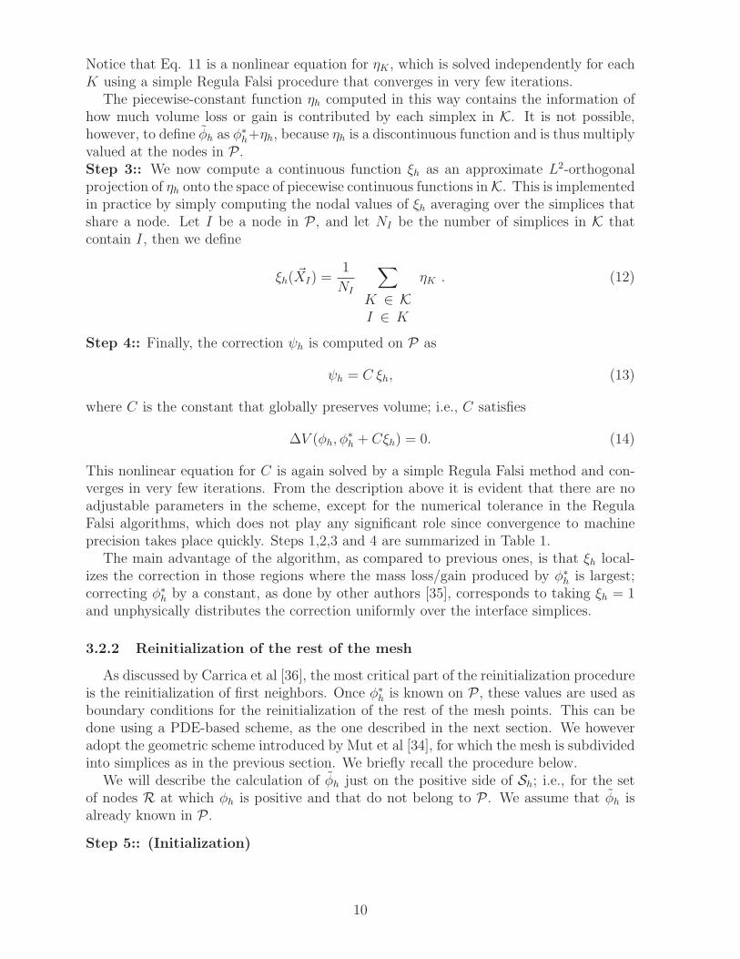
3.2.2 Reinitialization of the rest of the mesh

As discussed by Carrica et al [36], the most critical part of the reinitialization procedureis the reinitialization of first neighbors. Once φ∗

h is known on P , these values are used asboundary conditions for the reinitialization of the rest of the mesh points. This can bedone using a PDE-based scheme, as the one described in the next section. We howeveradopt the geometric scheme introduced by Mut et al [34], for which the mesh is subdividedinto simplices as in the previous section. We briefly recall the procedure below.

We will describe the calculation of φh just on the positive side of Sh; i.e., for the setof nodes R at which φh is positive and that do not belong to P . We assume that φh isalready known in P .

Step 5:: (Initialization)

10

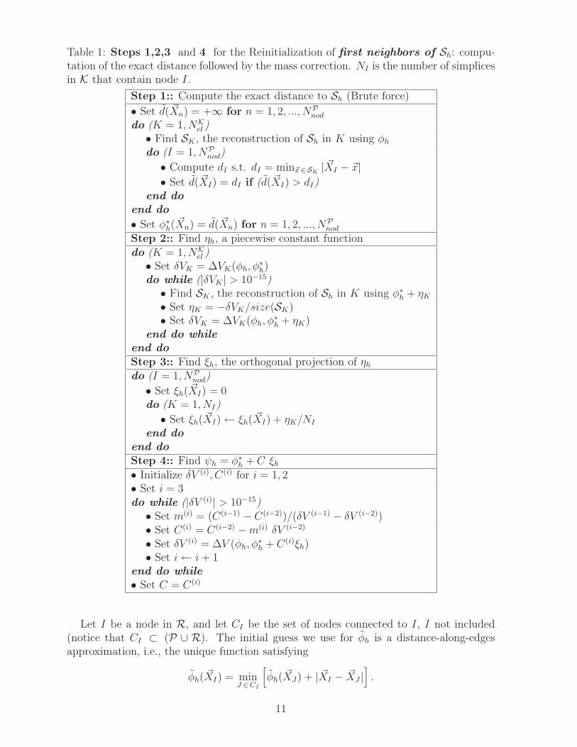
Table 1: Steps 1,2,3 and 4 for the Reinitialization of first neighbors of Sh: compu-tation of the exact distance followed by the mass correction. NI is the number of simplicesin K that contain node I.

Step 1:: Compute the exact distance to Sh (Brute force)

• Set d( ~Xn) = +∞ for n = 1, 2, ..., NPnod

do (K = 1, NKel )

• Find SK , the reconstruction of Sh in K using φh

do (I = 1, NPnod)

• Compute dI s.t. dI = min~x∈SK| ~XI − ~x|

• Set d( ~XI) = dI if (d( ~XI) > dI)end do

end do

• Set φ∗h(~Xn) = d( ~Xn) for n = 1, 2, ..., NP

nod

Step 2:: Find ηh, a piecewise constant functiondo (K = 1, NK

el )• Set δVK = ∆VK(φh, φ

∗h)

do while (|δVK | > 10−15)• Find SK , the reconstruction of Sh in K using φ∗

h + ηK

• Set ηK = −δVK/size(SK)• Set δVK = ∆VK(φh, φ

∗h + ηK)

end do whileend doStep 3:: Find ξh, the orthogonal projection of ηh

do (I = 1, NPnod)

• Set ξh( ~XI) = 0do (K = 1, NI)

• Set ξh( ~XI)← ξh( ~XI) + ηK/NI

end doend doStep 4:: Find ψh = φ∗

h + C ξh• Initialize δV (i), C(i) for i = 1, 2• Set i = 3do while (|δV (i)| > 10−15)• Set m(i) = (C(i−1) − C(i−2))/(δV (i−1) − δV (i−2))• Set C(i) = C(i−2) −m(i) δV (i−2)

• Set δV (i) = ∆V (φh, φ∗h + C(i)ξh)

• Set i← i+ 1end do while• Set C = C(i)

Let I be a node in R, and let CI be the set of nodes connected to I, I not included(notice that CI ⊂ (P ∪ R). The initial guess we use for φh is a distance-along-edgesapproximation, i.e., the unique function satisfying

φh( ~XI) = minJ ∈CI

[

φh( ~XJ) + | ~XI − ~XJ |]

.

11

In the process of initializing φh with this option, the elements can be ordered so as torender the algorithm more effective. Also, if one wants to calculate φh up to a distance δfrom Sh, one simply initializes φh as equal to δ over R.Step 6:: (Evaluation) The simplices in the mesh, excepting those in K, are swept untilφh no longer changes. For each simplex, and for each node J of the simplex (coordinates

denoted by ~XJ), φh is interpolated linearly on the opposite face FJ , using the currentvalues at the nodes. Then, a tentative new value ηJ of φh at node J is calculated as

ηJ = min~x∈FJ

[

φh(~x) + | ~XJ − ~x|]

. (15)

Finally, φh( ~XJ) is updated to the value ηJ if the current value is greater than ηJ . This isilustrated in figure 4 and in Table 2 we summarize both procedures.

~x→ Intersection with FJ

First Neighbors of Sh

Sh → Zero-level set of φh

Th → Finite element partition of Ω

~XJ

FJ ~x

| ~XJ − ~x|φh(~x)

φh( ~XJ) = min~x∈FJ

[

φh(~x) + | ~XJ − ~x|]

Second Neighbors of Sh

Sh

Figure 4: Schematic of Step 6:: (Evaluation) for the reinitialization of the rest of mesh.

3.3 PDE-based redistancing scheme

For the sake of completeness we briefly describe the PDE-based redistancing methodthat will be used for comparison, together with its discretization as proposed by Peng etal [6].

Let φ0 be a level set function with zero-level set denoted by S. Our aim is to computefrom this initial data φ0 an approximation φ for the distance function d to the zero–levelset S of φ0, defined as in (6) (with φh replaced by φ0 and Sh replaced by S)The property ‖∇d‖ = 1 motivates the redistancing method in which the following hyper-bolic partial differential equation (PDE) is solved

∂φ

∂τ+ sign(φ0)

(

‖ ∇φ ‖ −1)

= 0 in Ω,

(16)

φ(~x, 0) = φ0(~x),

12

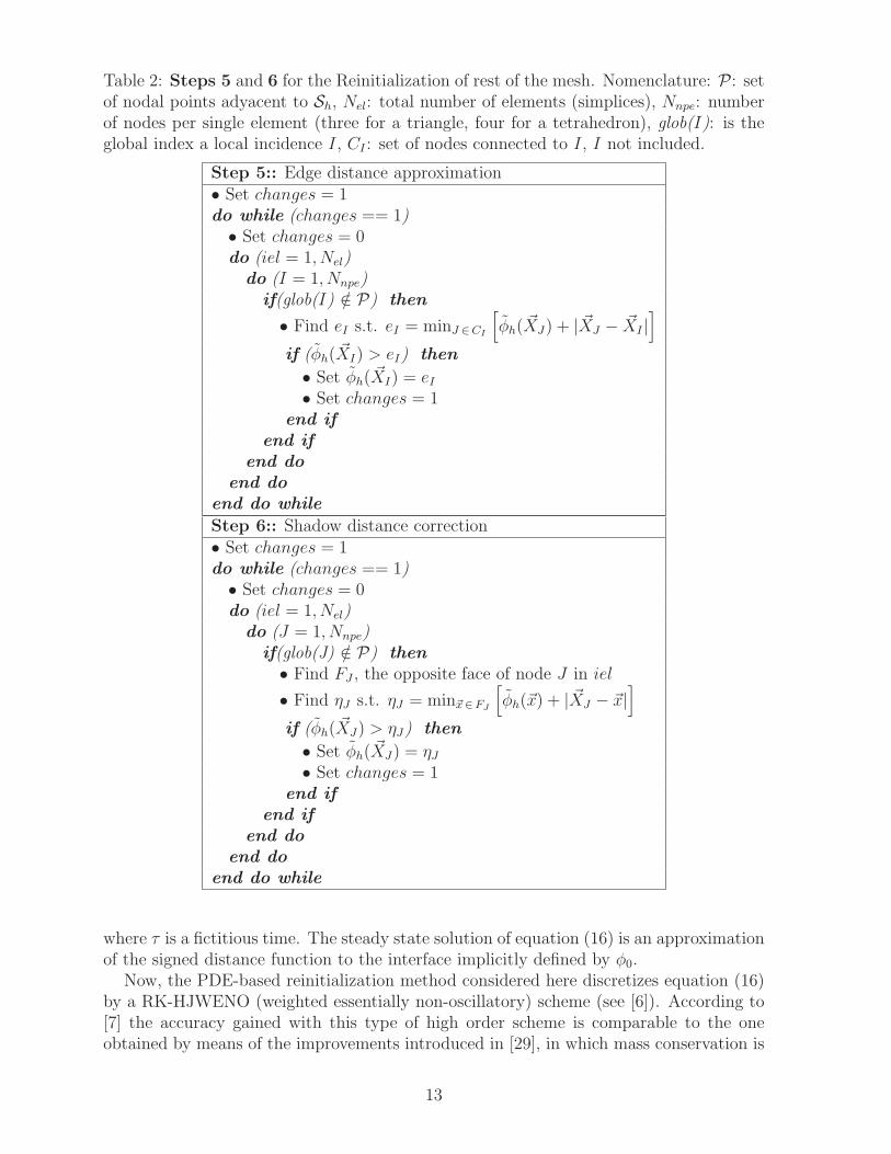
Table 2: Steps 5 and 6 for the Reinitialization of rest of the mesh. Nomenclature: P : setof nodal points adyacent to Sh, Nel: total number of elements (simplices), Nnpe: numberof nodes per single element (three for a triangle, four for a tetrahedron), glob(I): is theglobal index a local incidence I, CI : set of nodes connected to I, I not included.

Step 5:: Edge distance approximation• Set changes = 1do while (changes == 1)• Set changes = 0do (iel = 1, Nel)

do (I = 1, Nnpe)if(glob(I) /∈ P) then

• Find eI s.t. eI = minJ ∈CI

[

φh( ~XJ) + | ~XJ − ~XI |]

if (φh( ~XI) > eI) then

• Set φh( ~XI) = eI

• Set changes = 1end if

end ifend do

end doend do while

Step 6:: Shadow distance correction• Set changes = 1do while (changes == 1)• Set changes = 0do (iel = 1, Nel)

do (J = 1, Nnpe)if(glob(J) /∈ P) then• Find FJ , the opposite face of node J in iel

• Find ηJ s.t. ηJ = min~x∈FJ

[

φh(~x) + | ~XJ − ~x|]

if (φh( ~XJ) > ηJ) then

• Set φh( ~XJ) = ηJ

• Set changes = 1end if

end ifend do

end doend do while

where τ is a fictitious time. The steady state solution of equation (16) is an approximationof the signed distance function to the interface implicitly defined by φ0.

Now, the PDE-based reinitialization method considered here discretizes equation (16)by a RK-HJWENO (weighted essentially non-oscillatory) scheme (see [6]). According to[7] the accuracy gained with this type of high order scheme is comparable to the oneobtained by means of the improvements introduced in [29], in which mass conservation is

13

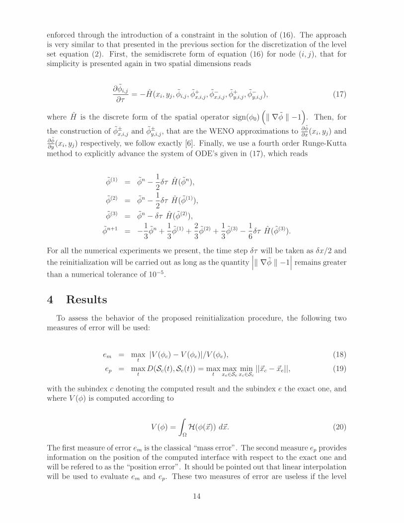
enforced through the introduction of a constraint in the solution of (16). The approachis very similar to that presented in the previous section for the discretization of the levelset equation (2). First, the semidiscrete form of equation (16) for node (i, j), that forsimplicity is presented again in two spatial dimensions reads

∂φi,j

∂τ= −H(xi, yj, φi,j, φ

+x,i,j, φ

−

x,i,j, φ+y,i,j, φ

−

y,i,j), (17)

where H is the discrete form of the spatial operator sign(φ0)(

‖ ∇φ ‖ −1)

. Then, for

the construction of φ±

x,i,j and φ±

y,i,j, that are the WENO approximations to ∂φ∂x

(xi, yj) and∂φ∂y

(xi, yj) respectively, we follow exactly [6]. Finally, we use a fourth order Runge-Kutta

method to explicitly advance the system of ODE’s given in (17), which reads

φ(1) = φn −1

2δτ H(φn),

φ(2) = φn −1

2δτ H(φ(1)),

φ(3) = φn − δτ H(φ(2)),

φn+1 = −1

3φn +

1

3φ(1) +

2

3φ(2) +

1

3φ(3) −

1

6δτ H(φ(3)).

For all the numerical experiments we present, the time step δτ will be taken as δx/2 and

the reinitialization will be carried out as long as the quantity∣

∣

∣‖ ∇φ ‖ −1

∣

∣

∣remains greater

than a numerical tolerance of 10−5.

4 Results

To assess the behavior of the proposed reinitialization procedure, the following twomeasures of error will be used:

em = maxt|V (φc)− V (φe)|/V (φe), (18)

ep = maxtD(Sc(t),Se(t)) = max

tmaxxe∈Se

minxc∈Sc

||~xc − ~xe||, (19)

with the subindex c denoting the computed result and the subindex e the exact one, andwhere V (φ) is computed according to

V (φ) =

∫

Ω

H(φ(~x)) d~x. (20)

The first measure of error em is the classical “mass error”. The second measure ep providesinformation on the position of the computed interface with respect to the exact one andwill be refered to as the “position error”. It should be pointed out that linear interpolationwill be used to evaluate em and ep. These two measures of error are useless if the level

14

set is not reasonably resolved by the mesh. We have thus chosen cases in which localfeature sizes of the level set are not smaller than the grid resolution. Finally, we mustmention that the reinitialization procedure will be applied every 10 time steps for all thesimulations to be presented.

4.1 Numerical Experiments in 2D

Two examples will be presented in the two dimensional case: the Zalesak’s problem([37]) and the stretching of a circle under a deformation vortex ([38]).

4.1.1 Zalesak’s disk

The initial data is a slotted disk centered at (0.5, 0.75) with a radius of 0.15, a slotwidth of 0.075 and a slot lenght of 0.25 in a unit square computational domain.

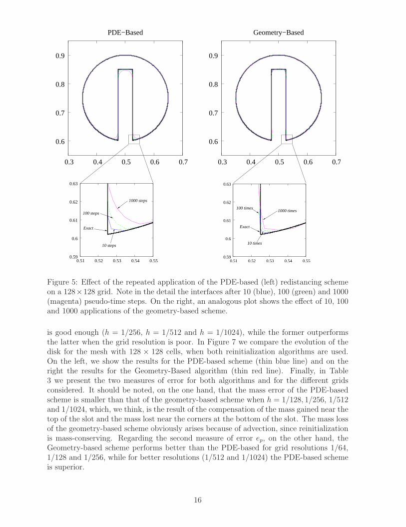
We first study the influence of the repeated application of the redistancing procedureswithout considering the advection step into account (zero convection velocity). Significantdifferences are observed between the two schemes. On the left of Fig. 5 we show theevolution of the PDE-based scheme towards its steady state, as a function of the numberof pseudo-time steps. The trend of the method to make sharp corners round is evident,together with the local loss of mass conservation. In fact, we believe that this behavior ofthe PDE-based redistancing scheme may be responsible of much of the numerical diffusionattributed to level-set-based methods. As the number of pseudo-time steps is increased (orequivalently, as the tolerance to achieving pseudo-steady state is tightened), the smoothingeffect of PDE-based reinitialization becomes stronger. The number of pseudo-time stepsperformed at each time step thus becomes a tunable parameter, for which the optimalchoice depends on the specific problem, mesh, etc.

On the right of Fig. 5 we show the effect of the repeated application of the geometry-based scheme. Notice that one application of this method is analogous to evolving thePDE-based method to steady state, so that no hidden tunable parameter exists. Repeatedapplication only occurs, as in this example, when the interface velocity is zero. Though thereinitialization distorts the interface, the distortion is much smaller than that caused bythe PDE-based method. Also, the mass is exactly conserved, as by design geometry-basedreinitialization is mass-conserving.

Now, in order to study the interaction between advection and reinitialization, we advectthe slotted disk by the following velocity field

ux =π

3.14(0.5− y),

(21)

uy =π

3.14(x− 0.5),

which represents a rigid body rotation with respect to (0.5, 0.5). The disk completes onerevolution after 6.28 units of time.

In figure 6 we compare the final stage of the Zalesak’s disk with the exact result after oneturn, for different grid resolutions. The time step for the first case (h = 1/64) is 6.28/600.For the rest of the grids we mantain the same Courant number. As it can be seen thegeometry-based scheme performs similarly to the PDE-based one when the grid resolution

15

1000 steps

10 steps

Exact

100 times

Exact

10 times

1000 times100 steps

0.6

0.7

0.8

0.9

0.3 0.4 0.5 0.6 0.7

PDE−Based

0.59

0.6

0.61

0.62

0.63

0.51 0.52 0.53 0.54 0.55 0.59

0.6

0.61

0.62

0.63

0.51 0.52 0.53 0.54 0.55

0.6

0.7

0.8

0.9

0.3 0.4 0.5 0.6 0.7

Geometry−Based

Figure 5: Effect of the repeated application of the PDE-based (left) redistancing schemeon a 128×128 grid. Note in the detail the interfaces after 10 (blue), 100 (green) and 1000(magenta) pseudo-time steps. On the right, an analogous plot shows the effect of 10, 100and 1000 applications of the geometry-based scheme.

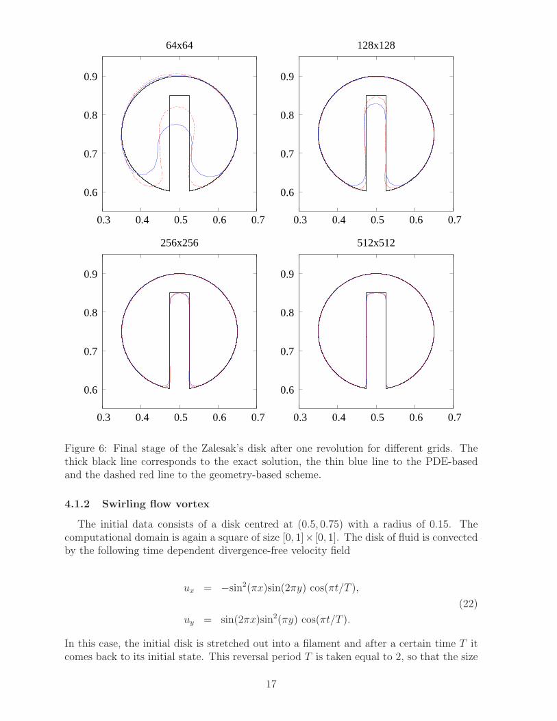
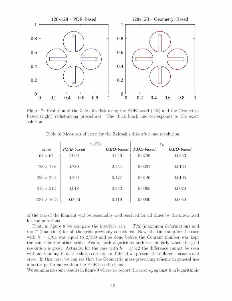
is good enough (h = 1/256, h = 1/512 and h = 1/1024), while the former outperformsthe latter when the grid resolution is poor. In Figure 7 we compare the evolution of thedisk for the mesh with 128 × 128 cells, when both reinitialization algorithms are used.On the left, we show the results for the PDE-based scheme (thin blue line) and on theright the results for the Geometry-Based algorithm (thin red line). Finally, in Table3 we present the two measures of error for both algorithms and for the different gridsconsidered. It should be noted, on the one hand, that the mass error of the PDE-basedscheme is smaller than that of the geometry-based scheme when h = 1/128, 1/256, 1/512and 1/1024, which, we think, is the result of the compensation of the mass gained near thetop of the slot and the mass lost near the corners at the bottom of the slot. The mass lossof the geometry-based scheme obviously arises because of advection, since reinitializationis mass-conserving. Regarding the second measure of error ep, on the other hand, theGeometry-based scheme performs better than the PDE-based for grid resolutions 1/64,1/128 and 1/256, while for better resolutions (1/512 and 1/1024) the PDE-based schemeis superior.

16

0.6

0.7

0.8

0.9

0.3 0.4 0.5 0.6 0.7

64x64

0.6

0.7

0.8

0.9

0.3 0.4 0.5 0.6 0.7

128x128

0.6

0.7

0.8

0.9

0.3 0.4 0.5 0.6 0.7

256x256

0.6

0.7

0.8

0.9

0.3 0.4 0.5 0.6 0.7

512x512

Figure 6: Final stage of the Zalesak’s disk after one revolution for different grids. Thethick black line corresponds to the exact solution, the thin blue line to the PDE-basedand the dashed red line to the geometry-based scheme.

4.1.2 Swirling flow vortex

The initial data consists of a disk centred at (0.5, 0.75) with a radius of 0.15. Thecomputational domain is again a square of size [0, 1]× [0, 1]. The disk of fluid is convectedby the following time dependent divergence-free velocity field

ux = −sin2(πx)sin(2πy) cos(πt/T ),

(22)

uy = sin(2πx)sin2(πy) cos(πt/T ).

In this case, the initial disk is stretched out into a filament and after a certain time T itcomes back to its initial state. This reversal period T is taken equal to 2, so that the size

17

0

0.2

0.4

0.6

0.8

1

0 0.2 0.4 0.6 0.8 1

128x128 − PDE−based

0

0.2

0.4

0.6

0.8

1

0 0.2 0.4 0.6 0.8 1

128x128 − Geometry−Based

Figure 7: Evolution of the Zalesak’s disk using the PDE-based (left) and the Geometry-based (right) redistancing procedures. The thick black line corresponds to the exactsolution.

Table 3: Measures of error for the Zalesak’s disk after one revolution.

em[%] ep

Mesh PDE-based GEO-based PDE-based GEO-based

64× 64 7.902 4.949 0.0709 0.0353

128× 128 0.789 2.254 0.0291 0.0134

256× 256 0.202 0.477 0.0126 0.0105

512× 512 0.018 0.253 0.0065 0.0070

1024× 1024 0.0046 0.119 0.0040 0.0050

of the tale of the filament will be reasonably well resolved for all times by the mesh usedfor computations.

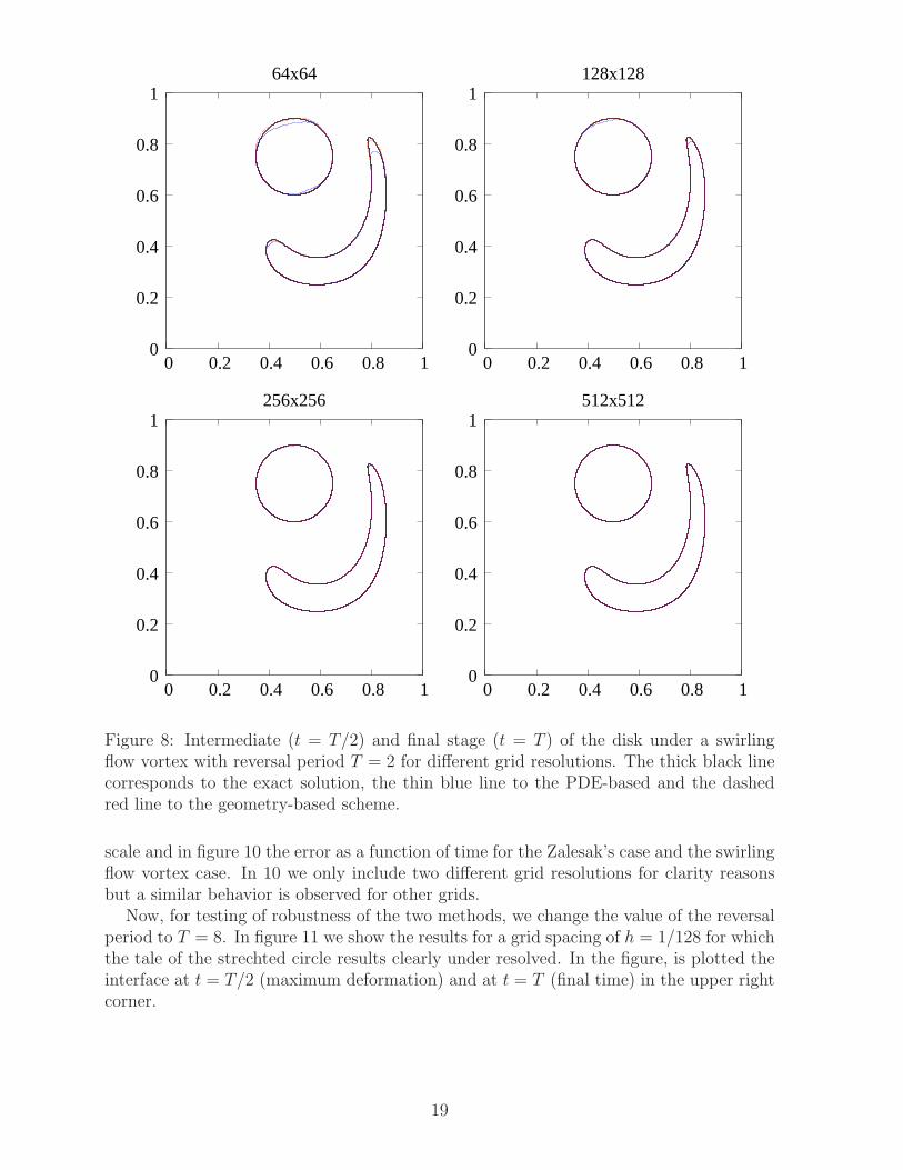
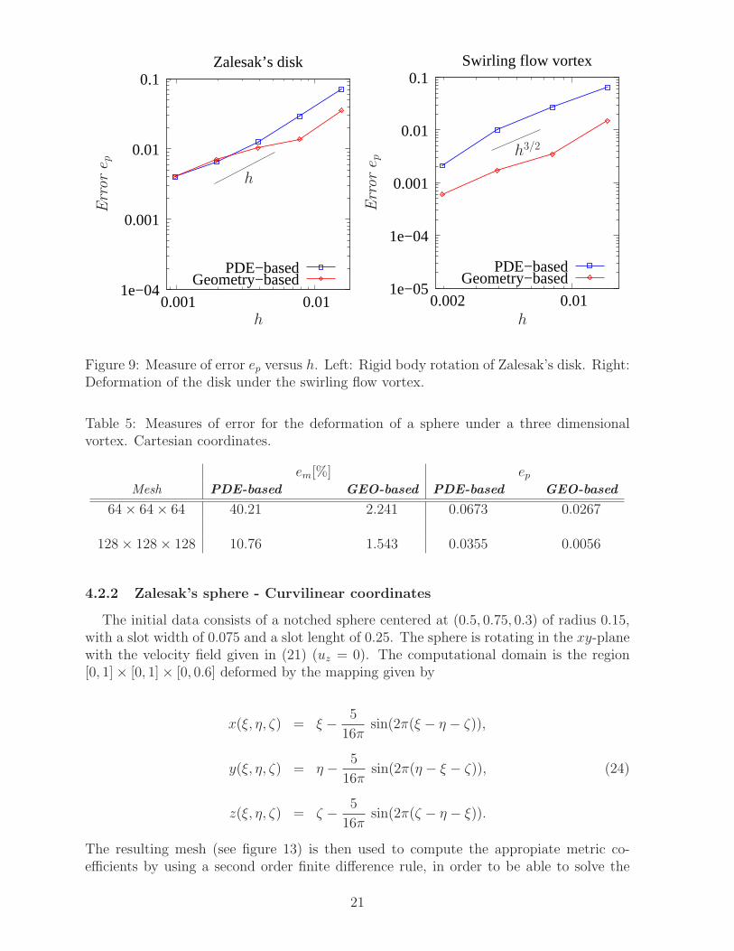
First, in figure 8 we compare the interface at t = T/2 (maximum deformation) andt = T (final time) for all the grids previouly considered. Now, the time step for the casewith h = 1/64 was equal to 2/300 and as done before the Courant number was keptthe same for the other grids. Again, both algorithms perform similarly when the gridresolution is good. Actually, for the case with h = 1/512 the difference cannot be seenwithout zooming in at the sharp corners. In Table 4 we present the different measures oferror. In this case, we can see that the Geometric mass-preserving scheme in general hasa better performance than the PDE-based scheme.We summarize some results in figure 9 where we report the error ep against h in logarithmic

18

0

0.2

0.4

0.6

0.8

1

0 0.2 0.4 0.6 0.8 1

64x64

0

0.2

0.4

0.6

0.8

1

0 0.2 0.4 0.6 0.8 1

128x128

0

0.2

0.4

0.6

0.8

1

0 0.2 0.4 0.6 0.8 1

256x256

0

0.2

0.4

0.6

0.8

1

0 0.2 0.4 0.6 0.8 1

512x512

Figure 8: Intermediate (t = T/2) and final stage (t = T ) of the disk under a swirlingflow vortex with reversal period T = 2 for different grid resolutions. The thick black linecorresponds to the exact solution, the thin blue line to the PDE-based and the dashedred line to the geometry-based scheme.

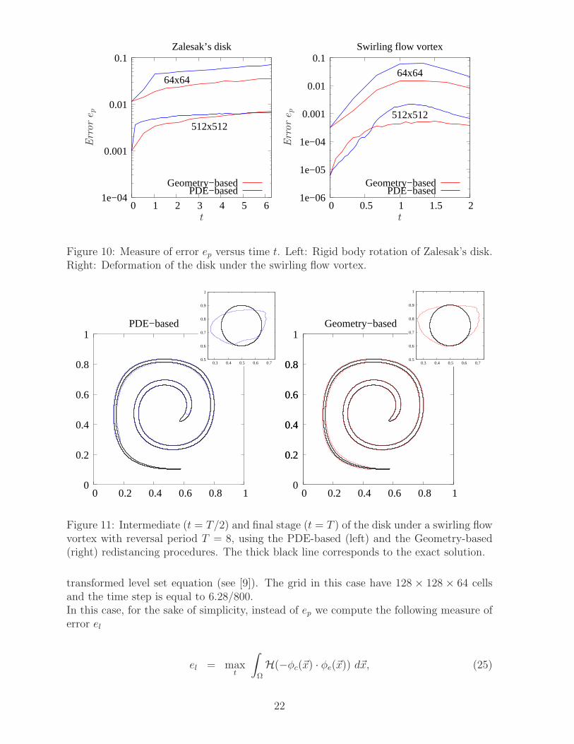
scale and in figure 10 the error as a function of time for the Zalesak’s case and the swirlingflow vortex case. In 10 we only include two different grid resolutions for clarity reasonsbut a similar behavior is observed for other grids.

Now, for testing of robustness of the two methods, we change the value of the reversalperiod to T = 8. In figure 11 we show the results for a grid spacing of h = 1/128 for whichthe tale of the strechted circle results clearly under resolved. In the figure, is plotted theinterface at t = T/2 (maximum deformation) and at t = T (final time) in the upper rightcorner.

19

Table 4: Measures of error for the streatching of a disk under a swirling flow vortex withreversal period T = 2.

em[%] ep

Mesh PDE-based GEO-based PDE-based GEO-based

64× 64 5.074 0.668 0.0641 0.0146

128× 128 1.643 0.118 0.0272 0.0028

256× 256 0.408 0.257 0.0100 0.0016

512× 512 0.086 0.136 0.0021 0.0005

1024× 1024 0.051 0.056 0.0028 0.0004

4.2 Numerical Experiments in 3D

For the three dimensional case, we present, on the one hand, results using Cartesiancoordinates and comparing both redistancing procedures and, on the other hand, resultsusing curvilinear coordinates with the Geometric mass-preserving redistancing schemecoupled with a finite difference second order TVD van Albada scheme for the transportof the level set function, similar to the one used in CFDShip-Iowa as already mentionedin the introduction.

4.2.1 Deformation vortex - Cartesian coordinates

In this example, the initial data consists simply of a sphere, centered at (0.35, 0.35, 0.35)and with a radius of 0.15. The computational domain is the unit cube. The sphere isthen convected by the following solenoidal field

ux = 2 sin2(πx)sin(2πy)sin(2πz) cos(πt/T ),

uy = −sin(2πx)sin2(πy)sin(2πz) cos(πt/T ), (23)

uz = −sin(2πx)sin(2πy)sin2(πz) cos(πt/T ),

again, as in the 2D case, the velocity field is modulated by a periodic function, such thatthe sphere will recover its initial state after a time T = 2.

In Table 5 we present the two measures of error, in this case just for two different gridsof 64×64×64 and 128×128×128 cells. The time step was taken equal to 2/400 and 2/800respectively. In figure 12 we plot the level set at different times for both algorithms forthe case with h = 1/128. In the top (red colour) are the results for the Geometry-basedredistancing and in the bottom (blue colour) the results for the PDE-based redistancing.From both, the figure and the table we can see that the Geometry-based redistancing hasa better performance.

20

1e−04

0.001

0.01

0.1

0.001 0.01

Zalesak’s disk

PDE−basedGeometry−based

Err

ore p

h

h

1e−05

1e−04

0.001

0.01

0.1

0.01

Swirling flow vortex

PDE−basedGeometry−based

0.002

Err

ore p

h

h3/2

Figure 9: Measure of error ep versus h. Left: Rigid body rotation of Zalesak’s disk. Right:Deformation of the disk under the swirling flow vortex.

Table 5: Measures of error for the deformation of a sphere under a three dimensionalvortex. Cartesian coordinates.

em[%] ep

Mesh PDE-based GEO-based PDE-based GEO-based

64× 64× 64 40.21 2.241 0.0673 0.0267

128× 128× 128 10.76 1.543 0.0355 0.0056

4.2.2 Zalesak’s sphere - Curvilinear coordinates

The initial data consists of a notched sphere centered at (0.5, 0.75, 0.3) of radius 0.15,with a slot width of 0.075 and a slot lenght of 0.25. The sphere is rotating in the xy-planewith the velocity field given in (21) (uz = 0). The computational domain is the region[0, 1]× [0, 1]× [0, 0.6] deformed by the mapping given by

x(ξ, η, ζ) = ξ −5

16πsin(2π(ξ − η − ζ)),

y(ξ, η, ζ) = η −5

16πsin(2π(η − ξ − ζ)), (24)

z(ξ, η, ζ) = ζ −5

16πsin(2π(ζ − η − ξ)).

The resulting mesh (see figure 13) is then used to compute the appropiate metric co-efficients by using a second order finite difference rule, in order to be able to solve the

21

1e−04

0.001

0.01

0.1

0 1 2 3 4 5 6

Zalesak’s disk

Geometry−basedPDE−based

512x512

64x64Err

ore p

t

1e−06

1e−05

1e−04

0.001

0.01

0.1

0 0.5 1 1.5 2

Swirling flow vortex

Geometry−basedPDE−based

512x512

64x64

Err

ore p

t

Figure 10: Measure of error ep versus time t. Left: Rigid body rotation of Zalesak’s disk.Right: Deformation of the disk under the swirling flow vortex.

0.5

0.6

0.7

0.8

0.9

1

0.3 0.4 0.5 0.6 0.7 0.5

0.6

0.7

0.8

0.9

1

0.3 0.4 0.5 0.6 0.7

0.2

0.4

0.6

0.8

0

0.2

0.4

0.6

0.8

1

0 0.2 0.4 0.6 0.8 1

PDE−based

0

0.2

0.4

0.6

0.8

1

0 0.2 0.4 0.6 0.8 1

Geometry−based

Figure 11: Intermediate (t = T/2) and final stage (t = T ) of the disk under a swirling flowvortex with reversal period T = 8, using the PDE-based (left) and the Geometry-based(right) redistancing procedures. The thick black line corresponds to the exact solution.

transformed level set equation (see [9]). The grid in this case have 128 × 128 × 64 cellsand the time step is equal to 6.28/800.In this case, for the sake of simplicity, instead of ep we compute the following measure oferror el

el = maxt

∫

Ω

H(−φc(~x) · φe(~x)) d~x, (25)

22

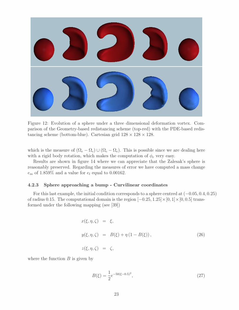
Figure 12: Evolution of a sphere under a three dimensional deformation vortex. Com-parison of the Geometry-based redistancing scheme (top-red) with the PDE-based redis-tancing scheme (bottom-blue). Cartesian grid 128× 128× 128.

which is the measure of (Ωe − Ωc) ∪ (Ωc − Ωe). This is possible since we are dealing herewith a rigid body rotation, which makes the computation of φe very easy.

Results are shown in figure 14 where we can appreciate that the Zalesak’s sphere isreasonably preserved. Regarding the measures of error we have computed a mass changeem of 1.859% and a value for el equal to 0.00162.

4.2.3 Sphere approaching a bump - Curvilinear coordinates

For this last example, the initial condition corresponds to a sphere centred at (−0.05, 0.4, 0.25)of radius 0.15. The computational domain is the region [−0.25, 1.25]×[0, 1]×[0, 0.5] trans-formed under the following mapping (see [39])

x(ξ, η, ζ) = ξ,

y(ξ, η, ζ) = B(ξ) + η (1−B(ξ)) , (26)

z(ξ, η, ζ) = ζ,

where the function B is given by

B(ξ) =1

2e−50(ξ−0.5)2 , (27)

23

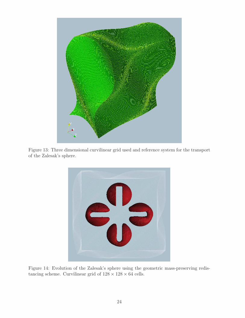
Figure 13: Three dimensional curvilinear grid used and reference system for the transportof the Zalesak’s sphere.

Figure 14: Evolution of the Zalesak’s sphere using the geometric mass-preserving redis-tancing scheme. Curvilinear grid of 128× 128× 64 cells.

24

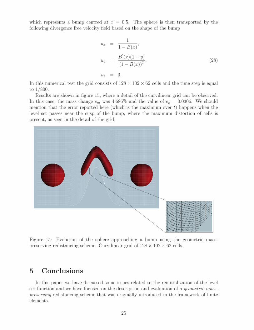
which represents a bump centred at x = 0.5. The sphere is then transported by thefollowing divergence free velocity field based on the shape of the bump

ux =1

1−B(x),

uy =B

′

(x)(1− y)

(1−B(x))2 , (28)

uz = 0.

In this numerical test the grid consists of 128× 102× 62 cells and the time step is equalto 1/800.

Results are shown in figure 15, where a detail of the curvilinear grid can be observed.In this case, the mass change em was 4.686% and the value of ep = 0.0306. We shouldmention that the error reported here (which is the maximum over t) happens when thelevel set passes near the cusp of the bump, where the maximum distortion of cells ispresent, as seen in the detail of the grid.

Figure 15: Evolution of the sphere approaching a bump using the geometric mass-preserving redistancing scheme. Curvilinear grid of 128× 102× 62 cells.

5 Conclusions

In this paper we have discussed some issues related to the reinitialization of the levelset function and we have focused on the description and evaluation of a geometric mass-preserving redistancing scheme that was originally introduced in the framework of finiteelements.

25

The geometric mass-preserving algorithm proposed can be used on an arbitrary tri-angulation of the computational domain, making it a very attractive tool to be used onany type of discretized domains such as the structured curvilinear grids widely used inCFD computations. A salient feature of the scheme is its simplicity and lack of adjustableparameters, which is an important difference as compared to other available methods.

The scheme is designed to preserve the mass (or the volume) delimited by the zero-levelset, which is defined by linear interpolation on a subdivision of the computational gridinto simplices.

In the numerical tests using Cartesian grids in two and three spatial dimensions, wehave observed in some cases a better performance of the geometric mass-preserving redis-tancing scheme and in some cases a better performance of the PDE-based method usedfor comparison, which is formally of higher order of convergence. This was illustratedqualitatively by means of plots of the level set and quantitatively be means of computingrelevant measures of error for level set methods. Numerical examples were then reported,showing that the performance of the method does not deteriorate when applied on arbi-trary curvilinear grids.

6 ACKNOWLEDGMENTS

Partial support of Agencia Nacional de Promocion Cientıfica y Tecnologica (Argentina),of Fundaca de Amparo a Pesquisa do Estado de Sao Paulo (Brazil) and of Conselho Na-cional de Desenvolvimento Cientıfico e Tecnologico (Brazil) are gratefully acknowledged.EAD and GCB also belong to Conicet (Argentina). RFA receives a fellowship from Con-icet (Argentina). Helpful comments were provided by Pablo Carrica.

References

[1] Osher S, Sethian J. Front propagating with curvature-dependent speed: algorithmsbased on Hamilton-Jacobi formulations. J. Comput. Phys. 1988; 79:12–49.

[2] Shu C, Osher S. Efficient implementation of essentially non-oscillatory shock-capturing schemes. J. Comput. Phys. 1988; 77:439–471.

[3] Shu C, Osher S. Efficient implementation of essentially non-oscillatory shock-capturing schemes II (two). J. Comput. Phys. 1989; 83:32–78.

[4] Harten A, Osher S. Uniformly high-order accurate essentially non-oscillatory schemesI. SIAM J. Numer. Anal 1987; 24:279–309.

[5] Harten A, Engquist B, Osher S, Chakravarthy S. Uniformly high-order accurateessentially non-oscillatory schemes III. J. Comput. Phys. 1987; 71:231–303.

[6] Jiang GS, Peng D. Weighted eno schemes for Hamilton-Jacobi equations. SIAM J.Sci. Comput. 2000; 21:2126–2144.

[7] Losasso F, Fedkiw R, Osher S. Spatially adaptive techniques for level set methodsand incompressible flow. Computers and fluids 2006; 35:995–1010.

26

[8] Yue W, Lin CL, Patel V. Numerical simulation of unsteady multidimensional freesurface motions by level set method. International Journal for Numerical Methodsin Fluids 2003; 42:853–884.

[9] Carrica P, Wilson R, Noack R, Xing T, Kandasamy M, Shao J, Sakamoto N, SternF. A dynamic overset, single-phase level set approach for viscous ship flows andlarge amplitude motions and maneuvering. 26th Symposium on Naval Hydrodynam-ics, Rome, Italy 2006; .

[10] Olsson E, Kreiss G. A conservative level set method for two phase flow. J. Comput.Phys. 2005; 210:225–246.

[11] Di Pietro D, Lo Forte S, Parolini N. Mass preserving finite element implementationsof the level set method. Applied Numerical Mathematics 2006; 56:1179–1195.

[12] Marchandise E, Remacle JF, Chevaugeon N. A quadrature-free discontinuousGalerkin method for the level set equation. J. Comput. Phys. 2006; 212:338–357.

[13] Sussman M, Fatemi E, Smereka P, Osher S. An improved level set method for in-compressible two-fluid flows. Computers and Fluids 1999; 20:1165–1191.

[14] Enright D, Losasso F, Fedkiw R. A fast and accurate semi-Lagrangian particle levelset method. Computers and Structures 2005; 83:479–490.

[15] Enright D, Fedkiw R, Ferziger J, Mitchell I. A hybrid particle level set method forimproved interface capturing. Computers and Structures 2002; 83:479–490.

[16] Strain J. Semi-Lagrangian methods for level set equations. J. Comput. Phys. 1999;151:498–533.

[17] Strain J. Tree methods for moving interfaces. J. Comput. Phys. 1999; 151:616–648.

[18] Zhaorui L, Farhad A, Shih T. A hybrid Lagrangian-Eulerian particle-level set methodfor numerical simulations of two-fluid turbulent flows. International Journal for nu-merical methods in fluids, (in press) DOI:10.1002/fld.1621 2007; .

[19] Hirt C, Nichols H. Volume of fluid (VOF) methods for the dynamics of free bound-aries. Aplied Numerical Mathematics 1981; 39:201–225.

[20] Sussman M. A second order coupled level set and volume of fluid method for com-puting growth and collapse of vapor bubbles. J. Comput. Phys. 2003; 187:110–136.

[21] Sussman M, Puckett E. A coupled level set and volume of fluid method for comput-ing 3D and axisymmetric incompressible two phase flows. J. Comput. Phys. 2000;162:301–337.

[22] Chopp D. Computing minimal surfaces via level set curvature flow. J. Comput. Phys.1993; 106:77–91.

[23] Tsitsiklis J. Efficient algorithms for globally optimal trajectories. IEEE Trans Au-tomat Control 1995; 40:1528–1538.

27

[24] Sethian J. A fast marching method for monotonically advancing fronts. Proc NatlAcad Sci 1996; 93:1591–1595.

[25] Sethian J. Fast marching methods. SIAM Rev 1999; 41:199–235.

[26] Chopp D. Some improvements of the fast marching method. SIAM Journal Sci.Comput. 2001; 23:230–244.

[27] Adalsteinsson D, Sethian J. A fast level set method for propagating interfaces. J.Comput. Phys. 1995; 118:269–277.

[28] Adalsteinsson D, Sethian J. The fast construction of extension velocities in level setmethods. J. Comput. Phys. 1999; 148:2–22.

[29] Sussman M, Fatemi E. An efficient, interface-preserving level set redistancing al-gorithm and its application to interfacial incompressible fluid flow. SIAM J. Sci.Comput. 1999; 20:1165–1191.

[30] Sussman M, Smereka P, Osher S. A level set approach for computing solutions toincompressible two-phase flow. J. Comput. Phys. 1994; 114:146–159.

[31] Lew A, Buscaglia G. A Discontinuous–Galerkin–based immersed boundary method.International Journal for Numerical Methods in Engineering 2008; 76:427–454.

[32] Russo G, Smereka P. A remark on computing distance functions. J. Comput. Phys.2000; 163:51–67.

[33] Min C, Gibou F. A second order accurate level set method on non-graded adaptivecartesian grids. J. Comput. Phys. 2007; 225:300–321.

[34] Mut F, Buscaglia G, Dari E. New mass-conserving algorithm for level set redistancingon unstructured meshes. Journal of Applied Mechanics 2006; 73:1011–1016.

[35] Aliabadi S, Tezduyar T. Stabilized-finite-element/interface-capturing technique forparallel computation of unsteady flows with interfaces. Comput. Methods Appl. Mech.Engrg. 2000; 190:243–261.

[36] Carrica P, Wilson R, Stern F. An unsteady single–phase level set method for viscousfree surface flows. Int. J. Numer. Meth. Fluids 2007; 53:229–256.

[37] Zalesak S. Fully multidimensional flux-corrected transport algorithms for fluids. J.Comput. Phys. 1979; 335-362:31.

[38] LeVeque R. High-resolution conservative algorithms for advection in incompressibleflow. SIAM Journal of Numerical Analysis 1996; 33:627–665.

[39] LeVeque R. Wave propagation algorithms for multidimensional hyperbolic systems.J. Comput. Phys. 1997; 131:327–353.

28