A GEOGRAPHY-SPECIFIC APPROACH TO ESTIMATING THE DISTRIBUTIONAL IMPACT OF HIGHWAY TOLLS: AN APPLICATION TO THE PUGET SOUND REGION OF WASHINGTON STATE

A Geography-Specific Approach to Estimating the DistributionalImpact of Highway Tolls: An Application to the Puget SoundRegion of Washington State

Robert D. Plotnick,University of Washington

Jennifer Romich,University of Washington

Jennifer Thacker, andBurst for Prosperity

Matthew DunbarUniversity of Washington

AbstractThis study contributes to the debate about tolls’ equity impacts by examining the potentialeconomic costs of tolling for low-income and non-low-income households. Using data from thePuget Sound metropolitan region in Washington State and GIS methods to map driving routesfrom home to work, we examine car ownership and transportation patterns among low-income andnon-low-income households. We follow standard practice of estimating tolls’ potential impactonly on households with workers who would drive on tolled and non-tolled facilities. We thenredo the analysis including broader groups of households. We find that the degree of regressivityis quite sensitive to the set of households included in the analysis. The results suggest thatdistributional analyses of tolls should estimate impacts on all households in the relevant region inaddition to impacts on just users of roads that are currently tolled or likely to be tolled.

Keywordstolls; equity; distributional impact; Puget Sound

Introduction and BackgroundIn planning regional transportation systems, policymakers balance overlapping andsometimes competing goals of effectiveness, cost-efficiency, environmental responsibilityand social equity. The increasingly popular strategy of tolling drivers on new facilities hasimplications for all these goals, and is one strategy among others for creating systems thatcan best move persons and goods through metropolitan areas.

In an era of limited state and local budgets and legislators’ reluctance to support higher fueltaxes or general tax increases, tolls on urban highways and bridges may be an attractivesource of funds for construction and maintenance of transportation infrastructure. Urbanpolicy makers are also gradually accepting well known arguments in the transportationresearch community that well designed tolls can help reduce congestion and air pollution bygiving residents incentives to use the highway system more efficiently. The most current

NIH Public AccessAuthor ManuscriptJ Urban Aff. Author manuscript; available in PMC 2011 August 7.

Published in final edited form as:J Urban Aff. 2011 August 7; 33(3): 345–366. doi:10.1111/j.1467-9906.2011.00551.x.

NIH

-PA Author Manuscript

NIH


NIH


federal surface transportation act, the 2005 Safe, Accountable, Flexible, EfficientTransportation Equity Act: A Legacy for Users (Public Law 109-59; SAFETEA-LU), gavemetropolitan planning organizations greater leeway to use congestion-based tolls as astrategy for reducing total miles driven. New or newly-tolled facilities now operate inCalifornia, Texas, Virginia and other states (Bhatt et al. 2008).

Along with tolls’ efficiency and revenue-raising benefits, their impacts on equity havebecome an important part of the debate about their acceptability and appropriate use. Criticsraise concerns that tolls are regressive.– That is, they cost low-income households a higherpercentage of their income than middle or upper income households. More broadly, policymakers should consider possible equity impacts of tolls alongside other spatial andtransportation topics with implications for low-income residents of metropolitan regions. Forinstance, for low-income workers who do not live close to employment centers, tolling couldexacerbate spatial mismatch (Kain 1992) by further increasing commuting costs. Debatesover tolling regimes in Europe – where tolling is more widely used – focus in part onwhether tolling constitutes a mechanism of social exclusion whereby lower-income residentsare less able to fully participate in normal social activities such as using public roads(Bonsall & Kelly, 2005).

This study contributes to the debate about tolls’ equity impacts by examining the potentialeconomic costs of tolling for low-income and non-low-income households. Using data fromthe Puget Sound metropolitan region in western Washington State, we examine carownership and transportation patterns among low-income and non-low-income households.We argue that conclusions about the regressivity of tolls are sensitive to which householdsare included and the spatial distribution of their residences and workplaces. Although theseideas are recognized in the prior literature, this article makes the conceptual advance oftranslating them into an empirical analysis.

The analysis improves on past research in two major ways. To our knowledge it is the firstto use Geographic Information Systems (GIS) methods to map driving routes from home towork in order to model possible tolling schemes. We determine the extent to which low-income households commute on highway segments that may have tolls in the future andcompare how frequently low-income and non-low-income households commute on eachsegment. Using a simple simulation based on a tolling regime already under publicconsideration, we confirm earlier findings that the financial costs of tolls are regressivelydistributed among users of the tolled facility.

Second, prior studies generally examine only drivers who use tolled facilities andoccasionally drivers who do not use tolled facilities. By omitting the many low-incomehouseholds without workers, or with commuters who do not use private vehicles, suchstudies overstate the effect of tolls on the entire low-income population. We follow standardpractice of estimating tolls’ potential impact only on households with workers who woulddrive on tolled and non-tolled facilities. We then redo the analysis including broader groupsof households. We find that the degree of regressivity is quite sensitive to the set ofhouseholds included in the analysis. These results suggest that distributional analyses of tollsshould estimate impacts on all households in the relevant region in addition to impacts onjust users of roads that are currently tolled or likely to be tolled. Doing so would accord withstandard practice in distributional studies of taxes and income support programs and wouldoffer more insight into how highway tolls may affect equity among all residents of theregion.

The remainder of this article has five sections. Section 1 reviews the literature on how tollsaffect equity, including what is known about tolls’ impacts on the financial status and

Plotnick et al. Page 2

J Urban Aff. Author manuscript; available in PMC 2011 August 7.

NIH


NIH


NIH


driving time of low-income households and on low-income households relative to middleand high income households. Section 2 describes the data set, which contains informationabout current residential and work locations of each household. It also describes a novelmethodology for exploiting this unusual information that uses geographic-specific routinganalysis to map current commuting routes. Section 3 first provides data on employment, carownership, commute mode and commuting routes of low-income and non-low-incomehouseholds. It then presents estimates of potential tolls’ cost to low-income and non-low-income households. Though results apply only to the Puget Sound region of WashingtonState, the study’s methods can be applied in any region where suitable data exist. In Section4 we consider how our conclusions about the distribution of the direct money cost of tollingmight be affected by monetizing the time savings resulting from congestion reduction,capturing changes in commuting behavior, or considering the full revenue system. The finalsection compares the findings to earlier research and discusses the additional informationgained when the analysis moves beyond users of tolled facilities to analyze more inclusivesets of households.

Section 1: Literature ReviewEquity in transportation has multiple dimensions – income, geographic, modal, gender andstill others – and can be examined at the individual, group and geographic level (Weinstein& Sciara 2004, Giuliano, 1994, Taylor, 2004, Ungemah 2007). This study analyzes incomeequity at the individual and group level, with groups defined by low-income status.

Assessing the income equity of a tolling regime requires analysis at several different levels.An initial question is: what are the regime’s likely financial and time impacts on low-incomehouseholds? Financial impacts include how much a typical low-income household wouldspend on tolls per year, the share of income spent on tolls, and how this spending mightaffect consumption of other goods and services. Time impacts include how much time low-income households would save because of congestion tolls or whether their travel timewould increase as they shift to public transportation or to non-tolled but longer or morecongested alternative routes.

A second question is that of vertical equity. How does tolls’ average burden as a share ofincome vary as household income rises? If the burden rises, falls or is constant, tolls arerespectively progressive, regressive or proportional. Assessing vertical equity requirescomparing the financial and time impacts for low-income households to those for middleand high income households. A related issue is whether the payment methods, deposits, andservice fees required by the collection technology (commonly an in-vehicle transponder)would disproportionately curtail low-income households’ access to transportation facilities.

Another aspect of income equity, horizontal equity, generally requires that tolls imposesimilar burdens on households with similar incomes. Assessing horizontal equity requireslooking within and across different types of households. Low-income households areheterogeneous and will hence be affected differently by tolling policies. A current low-wageworker who commutes daily via highways will be affected more than a non-worker orsomeone who currently walks to work.

A final set of concerns around the net distributional effects revolves around the poor as aclass or group. To determine whether low-income households generally experience benefitor detriment from a tolling regime, analysts must consider the full policy system, includingrevenue flows in the absence of a tolling regime and uses of toll revenues.



NIH


NIH


NIH


Facility- and Population-Specific FactorsAnswers about how much poor and non-poor persons will pay are necessarily project-andlocation-specific because they depend on the facilities subject to tolls, whether constant tollsor congestion tolls are imposed, the amount of the toll (and, for congestion tolls, how theamount changes), other relevant attributes of the specific tolling regime, and thedemographic characteristics of the region affected by the regime. Analysis must considerpopulation characteristics such as car use, employment and residential patterns. Differencesamong low-income households in whether they drive, whether and how they commute towork, and how far they live from work imply that the impacts of tolls will not be borneequally.

Tolls will mostly strongly affect car owners. Pucher and Renne (2003) use the 2001 NationalHousehold Travel Survey to examine travel patterns of low-income households (incomesbelow $23,000 in 2006 dollars).1 More than 26 percent of low-income households do nothave a car, compared to five percent of households in the next income level and less thantwo percent of households making more than $114,000 (2006 dollars). Among low-incomehouseholds that own cars, 65 percent have one, 24 percent have two, and 10 percent havethree or more (computed from Pucher and Renne, table 6). Even low-income householdswith no car report considerable auto use (34 percent of all trips in 2001), usually aspassengers in someone else’s car. Low-income households use cars for roughly 75 percentof their trips and public transit for only 4.6 percent of their trips. These figures are consistentwith an earlier and frequently cited study by Murakami and Young (1997) which found that84 percent of low-income households’ trips to work are made in private vehicles.

Employment patterns matter because travel to work is the least discretionary and the mostlikely to be tolled. Most low-income households contain at least one employed member, butthe percentage with workers is lower than for more affluent households (U.S. Census Bureau2009a). Commuting costs consume a disproportionately high share of low-income workers’earnings. One estimate suggests that working poor commuters who drive to work spend 8.4percent of their income on transportation costs, higher than the 4.5 percent of income spentby non-poor driving commuters (Roberto, 2008).

Where poor and non-poor workers live relative to employment opportunities is anotherconsideration. Although residential segregation by race has decreased over the 20th century,segregation by income level is both persistent and increasing (Jargowsky, 1996, Massey,Rothwell & Domina, 2009). Poverty is distributed unevenly over different neighborhoods,with areas of concentrated residential poverty giving rise to worries about spatial mismatch,in which low-income workers live away from employment areas. Nationwide, poverty isincreasing fastest in surburban and exurban areas (Kneebone, 2009). The distributionaleffect of a given toll regime will vary depending on whether it tolls routes between areas ofgreater or lesser poverty.

Findings on How Tolls Affect the Economic Well-being of the PoorPrior research suggests that tolling – in general – is regressive, but distributional impacts arerarely the sole focus of studies on tolling. A rigorous assessment of a tolling project’s equityimpacts requires complex data and highly sophisticated modeling of households’ potentialbehavioral responses to a specific tolling regime (Giuliano 1994). Since no study fully meetsthese requirements, one instead must identify the consensus of the major extant studies.

1Every study that we reviewed uses an income higher than the official federal poverty line to distinguish poor from non-poorhouseholds. Because of small sample size, in some studies the lowest income category extends well into the lower-middle and middleclass. Consequently, our discussion of each study uses the terms “poor” and “low-income” as defined by its author, not by the officialpoverty measure.



NIH


NIH


NIH


Most tolling research falls into one of two categories: projections of effects of hypotheticaltolling regimes or analyses of observed outcomes following enactment of tolls. Table 1 listsprevious studies for the U.S. and summarizes their implications or findings about thedistributional effects of tolls on low income populations. It does not include studies with nodata on income.

Small (1983) modeled the equity effects of three hypothetical peak expressway tolls andapplied the model to a sample of 118 highway commuters. In his study, when the toll’sfinancial cost and the value of time savings from less congestion are both counted, thelowest income group ($0–46,000 in 2005 dollars) has the largest absolute losses. Netbenefits were inversely related to income for all three tolls, a finding that is echoed in laterstudies that project possible effects based on current (non-tolled) travel patterns.

Small’s important early study illustrates later conclusions about the literature as a whole, inboth substantive findings and methodology. According to Richardson and Bae (1996) andGiuliano (1994), two major stylized facts about the income equity effects of tolls in theUnited States are 1.) High income drivers tend to benefit because they value their time morethan the increased cost of driving, and 2.) Low-income drivers and those who choose to nolonger using the tolled routes suffer losses.2Small’s 1983 analysis and many subsequentstudies have also relied on samples of current commuters, that is, persons already using theroutes to travel by automobile to employment.

Less is known about observed behavior in response to an actual toll. Three studies –Sullivan (2000, 2002) and Buris and Hannay (2004) – use observational data fromenactment of congestion tolls or HOT lanes (high occupancy tolled lanes, which allowsingle drivers to pay a premium to use high occupancy vehicle lanes). All three find thatusage of HOT lanes is positively correlated with income, but none of the studies havesufficient sample size to compare low-income users to others.

Transaction costs and mechanisms can restrict access as well. The paperwork, paymentmethods and deposits required by transponder programs present a significant obstacle tolow-income individuals’ access to tolled facilities because those persons are less likely tohave credit cards or bank accounts. Parkany (2005) found income is positively related totransponder ownership, toll road use, and frequency of use. Burris and Hannay (2004)speculate that the costs of purchasing and maintaining a transponder may have made theHouston QuickRide prohibitively expensive for some low-income drivers.

Revenue Use and Alternative Funding SourcesAnalysts generally share the view that toll’s negative impacts on low-income drivers couldpotentially be offset by how the revenues are used (Small 1992a, Santos & Rojey 2004,Safirova et al. 2005, Eliasson & Mattsson 2006). Direct redistribution of revenues on a per-capita basis or according to income can make all users better off and counteract theregressivity of tolls (Small, 1983; Franklin, 2007). While it may be possible, in principle, toredistribute the revenue so that all income groups gain, there are substantial political andadministrative obstacles to doing so.

Options to indirectly mitigate tolls’ regressive impacts include using the revenue to financeand subsidize public transportation improvements that disproportionately benefit poor

2Eliasson and Mattsson (2006) similarly conclude that tolls are most likely to be regressive where cars are widely used by both highand low-income individuals and low-income people have few alternatives in their modes of travel and less flexible work schedules.This, they observe, is often the case in American cities. They suggest that tolls may not be regressive in European cities, wheretransportation options and the residential locations of rich and poor generally differ from the American situation.



NIH


NIH


NIH


people (Prozzi et al. 2007, Weinstein & Sciara 2004), to support affordable housing optionsnear employment sites, or to give toll credits or exemptions to low-income drivers who mustdrive solo (Prozzi et al 2007, Weinstein & Sciara 2004). If implemented, these options couldhave important implications for the overall income equity of tolls. Yet none of them havebeen implemented in the United States. Under any redistribution plan, some low-incomeindividuals who are constrained to certain tolled routes will be worse off.3

While not redistributing the revenues implies that tolls are likely to be regressive, it isimportant to recognize the financing a project with tolls will generally impose fewer costson low-income persons than broad based consumption-oriented taxes such as the gas or salestax (Schweitzer & Taylor 2008). Since other taxes and fees may well be equally or moreregressive than tolls, to fully assess the equity effects of tolling one must compare tolls’effects to those of an alternate financing method in a no-toll scenario (Franklin 2007,Weinstein & Sciara 2004).

In sum, our review of the literature identified factors needed to evaluate the impact of atolling regime on low-income populations: a.) car ownership, b.) employment, c.) pre- andpost-toll travel patterns, d.) economic impacts due to pricing, e.) impacts due to collectionmechanisms and e). larger revenue considerations. Most empirical studies are based onsamples of current car-owning, employed commuters and examine one or two of thesefactors, (usually travel patterns and economic impacts).

Section 2: Data and methodologyOur empirical strategy deals with three of the factors identified above: car ownership,employment and pricing impacts. Using a unique geographic-specific routing analysis, wemap current commuting routes and make the assumption that they are the best possibleestimate of post-toll travel patterns. We draw on this mapping to estimate the impact ofpotential tolls on low-income and non-low-income households in the Puget Sound region.4

This method assumes that tolls do not affect current commuting patterns. We make thisassumption in view of data limitations. Because generally accepted models of travelbehavior imply that tolls induce some drivers to change modes, routes or other relevantbehaviors, tolls’ financial costs for both poor and non-poor households will be lower thanreported in this study.

Definition of low-incomeThis analysis defines low-income persons as those living in households with income at orbelow 200 percent of the official federal poverty line. The official poverty line uses a set ofdollar value thresholds that vary by family size and composition, but not geographically.The U.S. Census Bureau annually updates the thresholds for inflation using the ConsumerPrice Index for All Urban Consumers (CPI-U). In 2009, the official threshold for a family ofthree was $18,310. For four, it was $22,050.

We examine low-income persons rather than officially poor persons for several reasons.First, critics argue that the federal poverty thresholds are too low, particularly in high-costareas such as the Puget Sound (Blank, 2008; Pearce & Brooks, 2001). Second, a number ofimportant programs that assist needy persons implicitly acknowledge that the official

3Net revenues from London’s cordon toll are spent on improved bus services. Better services may mitigate the toll’s regressivity butdo not directly compensate specific low-income drivers who either pay substantial tolls or incur additional time costs.4Since collection mechanisms and other revenue issues can only be evaluated in the context of a specific tolling plan, these factors arebeyond the scope of this study.



NIH


NIH


NIH


thresholds are too low by setting their income eligibility thresholds higher than the officialpoverty line by as much as 300 percent (e.g. Head Start, food stamps, School LunchProgram, State Child Health Insurance Program). Third, the small number of officially poorhouseholds in the study’s key data file would lead to imprecise estimates. Last, near-poorhouseholds share many characteristics with poor households that contain workers. Researchshows that many households that are poor in one year may become near-poor the next yearand vice versa as household income fluctuates (Cellini, McKernan, & Ratcliffe, 2008).Because households with workers are those that commute, looking at both poor and near-poor may be more informative

DataThe study uses two data sets. Descriptive information about the low-income population,employment, travel time to work, car ownership, and commute mode comes from the 2007American Community Survey (ACS) Public Use Microdata Sample files for WashingtonState’s Puget Sound region: King, Pierce, Snohomish and Kitsap counties. This data setincludes 34,106 individuals in 14,911 households. The findings we report use the sampleweights, so they are representative of the population at large.

The key data set is the Puget Sound Regional Council’s 2006 Household Activities Survey(HAS). The Council commissioned the HAS to provide information on why householdsmake the choices that they do regarding travel behavior. The survey includes 4,746households in the Puget Sound region.

Mapping Commuting Routes—One of the HAS’s most valuable features is that itincludes both basic demographic information and exact (longitude and latitude) home andwork location for nearly all employed respondents. To map workers’ commuting routes, wemerged the demographic and latitude-longitude information into a GIS database. We createdand applied a mapping algorithm that assigned the most likely route between each home andwork pair. We manually checked assigned routes against Google Maps to identifyimplausible routes, and made hand edits as needed. This route information captured thedistribution of commuting trips on both major and minor roads. By combining the route anddemographic information, we were able to identify low-income and non-low incomeworkers most likely to use routes that may be tolled in the future.

Limitations of the Household Activities Survey—The HAS has two importantlimitations. It was designed to accurately represent the distribution of travel modes in thePuget Sound Region, not the distribution of income of users of each mode. Considerablecare was taken to oversample transit users. Similar care was not exercised in sampling poorand low-income households and, consequently, they are underrepresented.

Second, the data on income is weak. Household income is reported in broad categories – <$10,000, $10,000–19,999, etc. This crude measure makes it difficult to categorize somehouseholds as low-income or not with certainty.

We dealt with this problem with a simple procedure best explained by example. Consider afamily of four with two children. Suppose it reported a 2006 income in the $30,000–39,999range or a lower one. Since 200% of that family’s 2006 poverty line was $40,888, we canunambiguously classify it as low-income. If its reported income was in the $50,000–59,999range or higher, it is unambiguously non-low-income. If its income fell between $40,000and $49,999, where we cannot be certain about its low-income status, we assume it was low-income. Though this procedure overestimates the number of low-income families, since theerror can never exceed $10,000 we know that all these ambiguous families are notfinancially well off.



NIH


NIH


NIH


Notwithstanding the HAS’s limitations, its detailed data on home and work location providea valuable but rarely available resource for understanding the distributional effects of tolls.See (author citation 2009) for a more detailed discussion of the HAS limitations andsuggestions for research designs that could produce data even better suited to our questions.

Section 3: Empirical FindingsThis section presents new evidence about car ownership, employment and travel patterns.

Low-income and Non-low-income Populations in the Puget Sound RegionIn 2007 19.2 percent of all households in the four county Puget Sound region fell belowtwice the poverty line. The corresponding national rate was 32.8 percent (U.S. CensusBureau, 2009b). The region’s lower rate likely reflects its higher wage rates and better-than-average economic conditions at that time.

Employment, Car Ownership and Commute ModeBecause commuting is the major non-discretionary transportation activity, employment andcommute patterns are key for understanding potential impacts of tolls. Persons drive forother reasons, but generally have more flexibility in scheduling and getting to and from non-work activities.

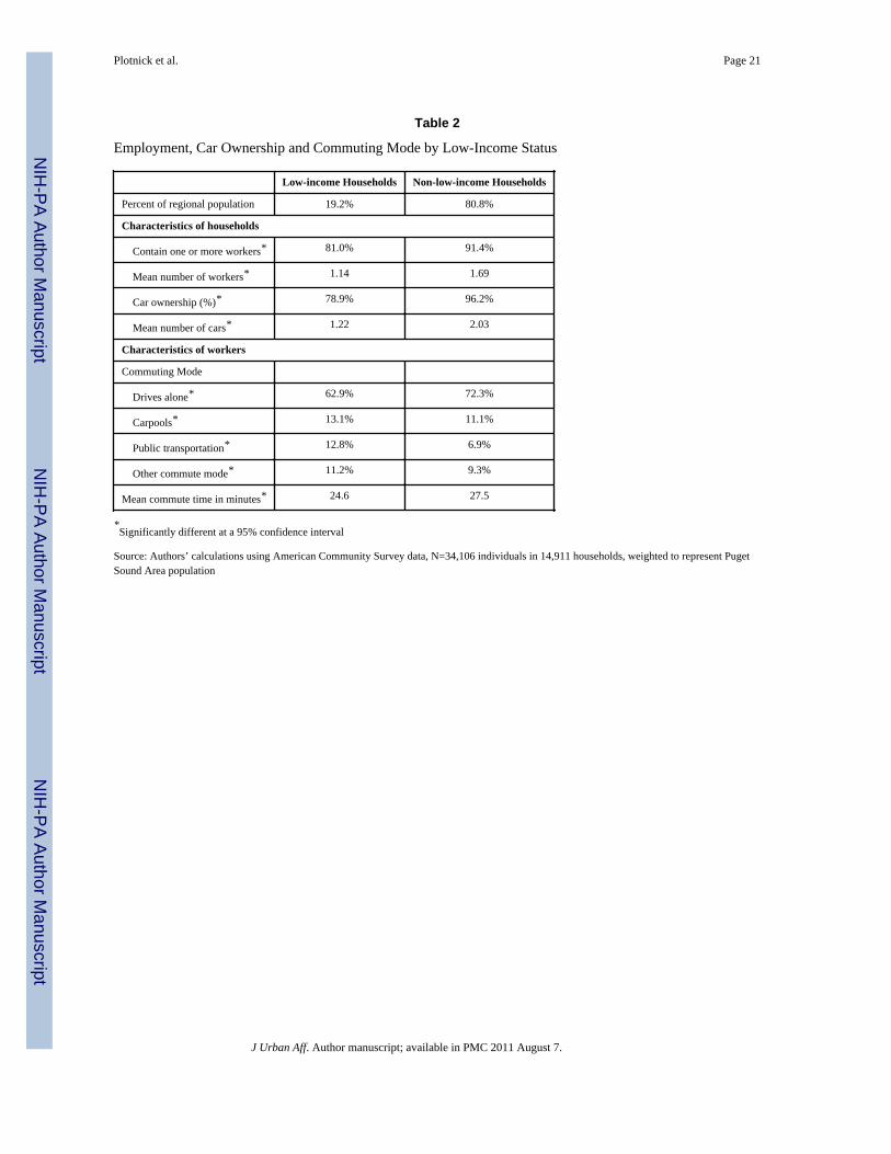
Table 2 shows information on employment and commuting among Puget Sound householdsbelow and above twice the poverty line. Eighty-one percent of low-income households and91 percent of non-low-income households contain at least one worker. Seventy-nine percentof low-income households and 96 percent of non-low-income households own at least onecar. On average, a low-income household owns 1.2 cars and a non- low-income householdowns 2.0.

Workers who currently commute via single occupancy vehicles are likely to be mostaffected by any new tolling regime. The bottom panel of Table 2 shows commute mode.Driving to work alone is most common, with 63 percent of low-income individuals and 73percent of non- low-income individuals commuting in this way. Low-income workers areslightly more likely to carpool than non-low-income workers (13.1 vs. 11.1 percent), andmore likely to use public transportation (12.8 percent vs. 6.9 percent) or other modes such aswalking or biking (11.2 vs. 9.3 percent). On average, low-income persons spend 24.6minutes commuting, or about two minutes less than non-low-income persons.

Table 2 confirms what other research has demonstrated: low-income persons in the PugetSound Region are less likely than their non-low-income counterparts to use a personalvehicle to get to work, although considerably more than half still manage to do so. Low-income persons are more likely to commute via public transportation or other modes thatwould not be subject to tolls. These facts imply that tolling is likely to affect a smallerpercentage of low-income persons than non-low-income persons in the region.

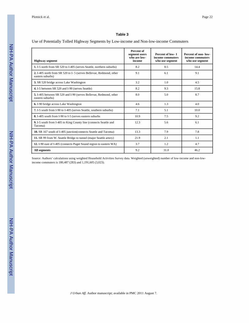
Commuting Routes of Low-Income and Non-Low-Income WorkersTo assess the impact of different toll scenarios, we focused on 12 segments of the region’shighway system for which tolls have already been discussed or implemented, or that appearto be plausible candidates for congestion tolls. Each segment extends over a different sectionof the six major highways in King County: I-5, I-405, I-90, SR 520, SR 167, and SR 99.Figure 1 shows all segments, which are described in table 3. They include, for example, thebridges across Lake Washington which connect Seattle and the affluent eastern suburbs



NIH


NIH


NIH


(segments 3 and 6). The stretch of I-5 between its junction with I-405 on the north and SR520 (the northern bridge across the lake) on the south is another (segment 1).

Figure 1 displays the trip density for all commuters in Puget Sound based on the routesestimated by our mapping procedure. Thicker lines indicate greater numbers of commuterson a given route. Not surprisingly, the most heavily used routes (1, 4 and 7) are segments ofthe interstate highway (I-5) adjacent to downtown Seattle. Shading within the lines indicatesthe percentage of users who are low-income. The most heavily-used routes have between 5and 10 percent low-income drivers. On the two east-west bridges, segment 3 and segment 6,fewer than 5 percent of all commuters are low-income.

Figure 2, derived with the GIS methods described earlier, shows the use of the 12 segmentsby both low-income and non-low-income commuters. More than two-thirds of low-incomecommuters use routes that include no segments. Twenty-two percent of low-incomecommuters use one or two segments; only nine percent use three or more. Tolling all 12segments, therefore, would increase out-of-pocket expenditures for no more than 31 percentof low-income commuters. Though the modal non-low-income commuter also uses nosegments, 32 percent of such commuters’ routes include one or two segments and 14 percentinclude three or more.

Column 1 of Table 3 reports the share of each segment’s users that is low-income. Thebottom row shows that low-income commuters account for 9.2 percent of all segment users.For segments 9–11, the shares of users with low incomes are three to twelve percentagepoints higher than 9.2 percent. That is, users of segments 9–11 are relatively more likely tobe low-income. The higher share of low-income users is especially pronounced for segment11. Users of segments 3 and 6 – the bridges across Lake Washington – are much less likelyto be low-income. For the other seven segments, the rate of use by low income commuters iswithin two percentage points of the overall rate.

These findings imply that tolls on segments 3 and 6 would be less regressive than a toll onany other segment. At the other extreme, a toll on segment 11 would be mostdisproportionately borne by low-income commuters.

The rightmost two columns of Table 3 report the proportion of low income and non-low-income commuters that use each segment. The base for the percentages is total number oflow-income or non-low income commuters, including those who use no segments. Hardlyany low income commuters use the two bridges (segments 3 and 6) or segment 12.5 Non-low-income commuters are also least likely to drive these four segments. Among low-income commuters only segments 1, 4, 8 and 10 have a rate of use greater than sevenpercent. No segment attracts more than 9.3 percent of low-income commuters or 15.8percent of non-low-income drivers.6 Tolling one or two segments would, consequently,impose financial costs on a small fraction of all low-income commuters. Tolling the twobridges, which is most practical and politically feasible, would affect less than three percentof low-income commuters.

5Note that though only 2.1 percent of low-income commuters use segment 11, even a smaller percentage of non-low-incomecommuters uses it. This is why the users of segment 11 are disproportionately low-income.6Since only 31 percent of low-income commuters and 46 percent of non-low-income commuters drive on one or more segments, thelow use of each segment by both income groups is to be expected. If we restrict the base to the number of low-income or non-lowincome commuters who use at least one segment, each column’s percentages will increase by the same factor (1/.31 or 1/.46), but theirratios will not change.



NIH


NIH


NIH


Toll Cost Estimates for Low-income and Non-low-income HouseholdsThe estimates of low-income and non-low-income households’ use of potentially tolledsegments allow us to project the potential annual cost of tolls for both groups and assesswhether tolls would cost a disproportionate share of low-income households’ income. Weconsider two scenarios.7

Scenario 1 assumes that a $1 one-way toll is imposed on all 12 focal segments listed inTable 3. We estimate the annual cost of tolls under this regime for three nested groups ofhouseholds. The largest group is all households, regardless of whether anyone in ahousehold works, drives a private vehicle to work, or uses a tolled segment. The averagenumber of tolled segments used per day by low-income and non-low-income households is0.49 and 1.25.

The second group includes only households with at least one person who commutes in aprivate vehicle, regardless of whether he uses a tolled segment. The average number oftolled segments used per day by low-income and non-low-income households withcommuters is 0.84 and 1.48. Many households in the first and second groups would pay notolls.

The third group is further restricted to households with at least one person who drives aprivate vehicle on at least one tolled segment. All of these households would pay tolls. Theaverage number of segments driven per day for low-income and non-low-incomehouseholds in this group is 2.07and 2.78.

Scenario 2 assumes a $2 one-way toll only on one bridge (segment 3).8 We estimate theannual cost of this regime for the small group of households that actually use the bridge.

We compute the annual cost assuming 240 work days per year. In scenario 1 a commuterwho drives roundtrip on one segment would pay $1×2 (roundtrip) × 240 = $480 per segmentper year. We compare the financial burden of tolls for two illustrative families. One is afamily with an income of $15,600, which is the median income among all low-incomehouseholds. The second’s income is $76,350, which is median income among non-low-income households.9

The upper part of table 4 presents the results for scenario 1. Taken over all households ineach group, the average low-income household would pay $235 per year, or $365 less thanwhat a non-low income household would pay. The low-income household would pay 1.5percent of its income for tolls, compared to 0.8 percent for the non-low-income household.The low-income household’s burden is 1.88 times larger than the non-low-incomehousehold’s.

Among commuting households, the average cost is necessarily higher — $403 for the lowincome household (2.6 percent of income) and $710 (0.9 percent) for the non-low-incomehousehold. In absolute terms low-income households pay about $300 less. The low-incomehousehold’s burden has increased in relative terms. It is 2.89 times larger than the share paidby the non-low-income household.

7Washington and other states are most likely to devote toll revenues fully to the construction, improvement and maintenance of tolledfacilities and, if funds suffice, other transportation projects (Franklin 2007, Richardson & Bae 1996, Weinstein & Sciara 2004).Hence, neither scenario incorporates a use of toll revenue that might offset the distributional effects of the toll..8The bridge (SR 520) is approaching the end of its engineered life span. Washington State and King County have agreed to jointly tollit to help finance its replacement. Tolls will continue to be collected on the new bridge. The average one-way toll is currentlyprojected to be $2.16 (Seattle Times 2009).9We derived these values from the 2007 American Community Survey because the income categories in the HAS are too broad toprovide useful estimates.



NIH


NIH


NIH


For only those households with commuters who actually drive on tolled segments, theaverage yearly cost is much higher — nearly $1,000 for low-income households and morethan $1,300 for non-low-income households. This cost would absorb 6.4 percent of theillustrative low-income household’s income, or 3.76 times higher than the representativenon-low-income household’s burden of 1.7 percent.

Devoting 6.4 percent of income to tolls would force significant reductions in other types ofexpenditures and, hence, substantially reduce the economic well-being of low-incomehouseholds whose workers commute in private vehicles. In the absence of specific efforts tosubsidize low-income users of tolled segments, tolls would likely induce many of them toadopt less costly commuting arrangements.

The burden of tolling all segments would be highly unequal among both low-income andnon-low-income households in the Puget Sound region. Low-income and non-low-incomeusers of tolled segments would pay an average of about $1,000 and $1,300 per year. Non-users, of course, would pay nothing.

The lower part of Table 4 presents findings when only the bridge has tolls. The $2 one-waytoll would cost the small number of households that use the bridge $960 per year, or 6.2 and1.3 percent of the illustrative households’ incomes. Spending almost $1,000 on tolls wouldcertainly reduce the economic well-being of low-income users of the bridge and encouragethem to seek less costly commuting arrangements. While the financial impact would belarge for low-income users of the bridge, for low-income commuters overall the impactwould be a negligible $10 (0.06 percent of income) per year since only one percent of themactually use this route (table 3, row 3). Similarly, since less than one in twenty non-low-income commuters would pay tolls on the bridge, the impact among all non-low-incomecommuters taken together would also be negligible (again, 0.06 percent of income).

Section 4. Extrapolations on Travel Time, Route Choice Changes, and Other Factors Ourempirical results and simulated toll scheme show that the distributional effects of tollingdiffer by the choice of population universe as well as the spatial distribution of route users.In this section we assess how our conclusions would change if we considered three otherfactors commonly used in judging the equity and policy implications of tolling: time savingsfrom congestion reductions, route or other behavioral changes to commute patterns, and thefull revenue system.

Time savings—Whether and how to value any time saved due to reduced congestion is ahighly contested – yet important – aspect of deciding the costs, benefits and distributionaleffects of any transit change. How to assign value to commute time is contested for the“average” commuter (Calfee & Winston, 1998, Brownstone & Small, 2005), and the extantliterature provides particularly scant guidance for how to value time for lower- versushigher-income households. However, to ignore travel time is to assume it has no value,which seems unsupportable. For this reason, we calculated time savings for our focal route.Details of the calculations are in Appendix 1.

Any reduction in travel time on our focal segment would necessarily mainly benefit higher-income households, as more of them use the route. One approach is to value commute timeat the half the hourly wage rate and assume a substantial reduction in congestion-relateddelays. Doing so reduces net annual cost of the $2 one-way toll to $866 for the low-incomehousehold and to $501 for the high-income household. In fact, any of the commonmonetizing schemes in the literature would increase the regressivity of the toll, and evensmall differences in the value of time for low versus high income drivers make the tolling



NIH


NIH


NIH


scheme on net regressive even for the full universe of commuting and non-commutinghouseholds.

Route changes—The estimates do not take into account that some drivers may changeroutes, modes, and other relevant behaviors in response to the tolls and the associated costsof accessing tolled highways (need for credit card or bank account, deposits, service fees).To the extent that such changes occur, the financial costs for both low-income and non-low-income households would be lower than reported here and probably distributed differently,though the time costs would likely be higher.

We offer a simple thought experiment to examine how the findings on regressivity mightdiffer if we could adjust for changes in routes and other commuting behaviors induced bytolls. How much would low-income households need to reduce use of tolled routes (orswitch to mass transit or carpools, which would not require tolls) so that the share of theirincome spent on tolls equals that of non-low-income households? A situation of equal sharesis usually interpreted as distributionally neutral.

Suppose that in the full-system tolling regime non-low-income households did not reduceuse of tolled segments. Then, for all low-income households to pay the same share of theirincome in tolls as non-low-income households (0.8 percent from row one of table 4), theywould need to take 47 percent fewer trips on tolled segments.10 If we confine attention tolow-income commuting households or segment commuters, use would need to declinerespectively by 65 percent or 73 percent. Since a 47 percent reduction in use (much less 65or 73 percent) seems unlikely, a full-system tolling regime would almost surely remainregressive in financial terms after low-income households adjust their driving behavior.Moreover, the burden of longer driving times necessitated by using minor roads wouldpartially offset low-income households’ financial savings and move the overall regressivityback towards the initial estimate.11

Revenue—Washington State has one of the most regressive state tax structures in thecountry, due in large part to the absence of a state income tax. Households with annualincome below $20,000 pay an estimated 17.3% of their income in state property, sales, andexcise taxes, whereas higher income households (in the fourth quintile) pay only 9.5% oftheir income in taxes (Davis, Davis et al, 2009). If the revenue raised by tolling wouldsupplant funds from the state general fund, tolls would be more progressive.

Other considerations—Might there be benefits to tolling that favor low income peopleand thereby reduce the regressivity of an area-wide tolling regime? Recent research showsthat poor people in the Tampa, FL area are more likely to live near sources of air pollution(Stuart et al. 2009). In that case, any health benefits from traffic reductions and diversionsinduced by tolls would tend to disproportionately favor the poor and offset some of adversefinancial impacts. Given the site-specific nature of tolls’ financial impacts, variations in airquality, and low income neighborhoods’ proximity to major roads, the applicability of thisresult to the Puget Sound region and other metropolitan areas must be ascertained on a case-by-case basis. The size of any health benefits is not known.

10To derive this figure, note that 0.8 percent of the representative low-income household’s income is $125. The ratio of $125 to table4’s projected cost of $235 is .53. This means usage must fall by 47 percent.11If higher income households did reduce their use of tolled routes, low-income households would need even larger reductions in useto achieve distributional neutrality. For instance, if higher income households took 10 percent fewer trips on tolled segments, low-income users would need to reduce their use by 54, 69 and 75 percent.



NIH


NIH


NIH


Section 5. DiscussionIf we restrict attention to only households that drive on potentially tolled routes in the PugetSound region, we find that tolls would absorb one-sixteenth of the representative low-income household’s income. This significant burden would be 3.77 times larger than thatborne by the representative non-low-income household, a substantial degree of regressivity.Narrowing the focus to households that use the one bridge that will almost certainly betolled gives burdens of 6.2 and 1.3 percent. This raises the regressivity; the low-incomehousehold’s burden would be 4.77 times larger than the non-low-income household’s. Thispair of findings confirms the consensus from previous research that tolls are regressive –among users of tolled facilities, the portion of income paid in tolls is inversely related totheir incomes.

A more nuanced story emerges when one moves beyond the conventional focus on users oftolled facilities to analyze more inclusive sets of households. For all commuting households,regardless of whether they use potentially tolled routes, the ratio of the burdens falls to 2.89.For the broadest population – all households regardless of whether they commute – the ratiofalls further to 1.88, or half the ratio when the calculation includes only households that usepotentially tolled routes. As the analysis becomes more inclusive, the regressivity shrinks.

By looking beyond users of tolled facilities and including all low-income and non-lowincome households in the analysis, we further demonstrate that tolls are not borne equallyamong all low-income households, nor among all non-low-income households. Fully 69percent of low-income households and 56 percent of non-low-income households would payno tolls (table 3, bottom row). The 31 and 44 percent who do pay would incur significantburdens averaging 2.6 and 0.9 percent of income. Differences in whether householdmembers drive, whether they need to commute to work, how far they live from work, andthe specific roads they drive create these differences.

While such differences may raise equity concerns, on balance we suggest the differences areappropriate. If tolls are to reduce congestion (with less pollution as an accompanyingbenefit), they must give residents who drive the most heavily trafficked roads and bridgesincentives to use them more efficiently, whatever their incomes may be. All pricingmechanisms discriminate between those who desire a good or service and those who do not.Tolls are no different. Generally speaking, economic theory suggests that the broader socialgoals of poverty reduction and income redistribution are best pursued via tax, incometransfer and labor market policies, not by suppressing prices’ function of allocating scarceresources.

The lower panel of table 4 more strongly demonstrates that restricting the analysis to usersof a tolled route may present a greatly distorted picture of tolls’ distributional impact onmore inclusive populations. Taken over all low-income commuters, the burden of the bridgetoll is 0.06 percent of income. For all low-income households, the burden falls to 0.04percent. Because low-income commuters use the bridge much less often than non-low-income households (1.0 versus 4.5 percent of commuters) and a smaller proportion of low-income households have commuters, a toll on the bridge would be distributed roughlyproportionally or even slightly progressively across all households in the region.

This last finding has important implications for the choice of mechanism for financingconstruction of a new bridge or highway. In the case at hand, financing via tolls on thebridge would essentially be distributionally neutral. Doing so would be more equitable thanrelying on the typical alternatives – sales and gasoline taxes – which are clearly regressiveand would impose significant burdens on low-income households that do not use the bridge(Schweitzer & Taylor 2008). More widespread understanding of the argument that we



NIH


NIH


NIH


should compare the equity effects of tolls to the equity of the current system of funding, nota perfectly egalitarian one, might increase the acceptability of tolls.

Are there viable alternatives for reducing congestion that would not put as high a financialburden on poor users of facilities that would otherwise be tolled? Offering incentives andmounting public information campaigns to encourage more biking, walking, carpooling anduse of HOV lanes may have a role, but are unlikely to significantly reduce congestion.12Expanding bus, subway and light rail services may be more promising, but the costs ofdoing so are largely financed with earmarked taxes, not fares (user fees). Such taxes –typically on retail sales, gasoline or property – are generally regressive and burden the manypoor families that do not use these services. Ultimately the most effective way to reducecongestion, in our view, is to directly increase the cost of sole-occupancy driving.Congestion tolls are the most suitable means to do so.

Our general patterns that higher-income households are disproportionately likely to containhighway commuters would probably apply in other metro areas as well. The Puget Soundregion may be an extreme case, with a high proportion of high-income householdscommuting on that particular segment, but the general pattern likely holds.

We suggest that distributional analyses of tolls include all households in the relevant region,not just those that use roads that are currently tolled or likely to be tolled. Doing so wouldaccord with standard practice in distributional studies of taxes and income support programs,which take into account households that pay no taxes or even negative taxes (if they qualifyfor refundable tax credits that exceed their federal income tax liability), or receive noincome transfers. Such an approach would offer more insight into how equity effects differwithin income groups as well as between them, and how highway tolls affect region-wideequity.

AcknowledgmentsOur research was supported by a grant from the Washington State Department of Transportation. We thank DanCarlson, Mark Hallenbeck, Matthew Kitchen, Rachel Kleit, Paul Krueger, Kathy Lindquist, Kathleen McKinney,Jamie Strausz-Clark, and participants in the West Coast Poverty Center’s seminar series for helpful comments onthe study. We also thank Neil Kilgren of the Puget Sound Regional Council for providing us a copy of theCouncil’s 2006 Household Activities Survey and the Washington State Transportation Center (TRAC) at theUniversity of Washington for clerical support. The contents do not necessarily reflect the official views or policiesof the Washington State Transportation Commission, Washington State Department of Transportation, TRAC,Federal Highway Administration, or Puget Sound Regional Council, or the views of any of their employees.

ReferencesAuthor citation 2009.Bhatt, K.; Higgins, T.; Berg, JT.; Buxbaum, J.; Enarson-Hering, E. Final report prepared for Federal

Highway Administration. U.S. Department of Transportation; 2008 August. Value Pricing PilotProgram: Lessons Learned.

Blank RM. Presidential address: How to improve poverty measurement in the United States. Journal ofPolicy Analysis and Management. 2008; 27(2):233–254.

Burris, MW.; Hannay, RL. Transportation Research Record: Journal of the Transportation ResearchBoard. Transportation Research Board of the National Academies; 2004. Equity Analysis of theHouston, Texas QuickRide Project; p. 87-92.

Calfee, John; Winston, Clifford. The value of automobile travel time: implications for congestionpolicy. Journal of Public Economics. 1998; 69(1):83–102.

12These alternative modes are not practical for many trips and, to the extent they do succeed in moving some cars off congested roads,others seem to take their place.



NIH


NIH


NIH


Cambridge Systematics. Report prepared for the Federal Highway Administration. Cambridge, MA:2005. Traffic Congestion and Reliability: Trends and Advanced Strategies for CongestionMitigation. at http://ops.fhwa.dot.gov/congestionreport/

Cellini SR, McKernan SM, Ratcliffe C. The dynamics of poverty in the United States: A review ofdata, methods, and findings. Journal of Policy Analysis and Management. 2008; 27(3):577–605.

Davis, Carl; Davis, Kelly; Gardner, Matthew; Mclntyre, Robert S.; McLynch, jeff; Sapozhnikova,Alia. A Distributional Analysis of the Tax Systems in All 50 States. Washington, DC: Institute onTaxation and Economic Policy; 2009 November. Who Pays?.

Eliasson J, Mattsson LG. Equity Effects of Congestion Pricing: Quantative Methodology and a CaseStudy for Stockholm. Transportation Research Part A. 2006; 40:602–620.

Franklin, J. Decomposing the Distributional Effects of Roadway Tolls. Paper submitted for the 2007Annual Meeting of the Transportation Research Board; 2007.

Giuliano, G. Curbing Gridlock: Peak Period Fees to Relieve Traffic Congestion. TransportationResearch Board Special Report 242. Vol. 2. Washington, D.C: National Academy Press; 1994.Equity and Fairness Considerations of Congestion Pricing; p. 250-279.

Jargowsky P. Take the Money and Run: Economic Segregation in U.S. Metropolitan Areas. AmericanSociological Review. 1996; 61:984–998.

Kain JF. The Spatial Mismatch Hypothesis: Three Decades Eater. Housing Policy Debate. 1992; 3(2):371–460.

Kneebone, E. The Suburbanization of American Poverty. Washington, DC: Brookings Institution;2009.

Massey DS, Rothwel J, Domina T. The Changing Bases of Segregation in the United States. TheAnnals of the American Academy of Political and Social Science. 2009; 626(1):74–90.

Murakami, E.; Young, J. Daily Travel by Persons with Low-income. Paper submitted for the NationalPersonal Transportation Survey Symposium; Bethesda, MD. October 29th - 31st., 1997; 1997.

Parkany, E. Transportation Research Record: Journal of the Transportation Research Board.Transportation Research Board of the National Academies; 2005. Environmental Justice IssuesRelated to Transponder Ownership; p. 97-108.

Pearce, D.; Brooks, J. The Self-Sufficiency Standard for Washington State. Seattle, WA: WiderOpportunities for Women; 2001.

Pucher J, Renne JL. Socioeconomics of Urban Travel: Evidence from the 2001 NHTS. TransportationQuarterly. 2003 Summer;57(3):49–77.

Puget Sound Regional Council. Traffic Choices Study: Summary Report. 2008 April.Roberto, E. Commuting to Opportunity: The Working Poor and Commuting in the United States.

Washington, DC: Brookings Institution; 2008.Richardson, HB.; Bae, CC. The Equity Impacts of Road Congestion Pricing. In: Button, Kenneth J.;

Verhof, Erik T., editors. Road Pricing, Traffic Congestion and the Environment: Issues ofEfficiency and Social Feasibility. Cheltenham: Edward Elgar Publishing; 1998. p. 247-262.

Safirova, E.; Gillingham, K.; Harrington, W.; Nelson, P. Resources for the Future Urban ComplexitiesBrief 03-03. 2003 May. Are HOT Lanes a Hot Deal? The Potential Consequences of ConvertingHOV to HOT lanes in Northern Virginia.

Safirova, E.; Gillingham, K.; Harrington, W.; Nelson, P.; Lipman, A. Transportation Research Record:Journal of the Transportation Research Board. Transportation Research Board of the NationalAcademies; 2005. Choosing Congestion Pricing Policy: Cordon Tolls vs. Link Based Tolls; p.169-177.

Santos G, Rojey L. Distributional Impacts of Road Pricing: The Truth Behind the Myth.Transportation. 2004; 31:21–42.

Schweitzer L, Taylor BD. Just pricing: The distributional effects of congestion pricing and sales tax.Transportation. 2008; 35(6):797–812.

Seattle Times. [Accessed September 17, 2009] State won’t be ready on time, delays start of tolling on520 bridge. 2009. at http://seattletimes.nwsource.com/html/traffic/2009873777_520tollsl6m.html

Small K. The Incidence of Congestion Tolls on Urban Highways. Journal of Urban Economics. 1983;13:90–111.



NIH


NIH


NIH


http://ops.fhwa.dot.gov/congestionreport/

http://seattletimes.nwsource.com/html/traffic/2009873777_520tollsl6m.html

Small, K. Using the Revenues from Congestion Pricing. Paper prepared for the Congestion PricingSymposium, Sponsored by the Federal Highway Administration; June 10–12; 1992a.

Small, KA. Urban Transportation Economics, Fundamentals of Pure and Applied Economics Series.Vol. 51. Harwood Academic Publishers; New York: 1992b. Reprinted by Routledge, Abingdon,UK

Small, KA. Urban Transportation Economics, Fundamentals of Pure and Applied Economics Series.Vol. 51. Harwood Academic Publishers; New York: 1992b. Reprinted by Routledge, Abingdon,UK

Small, Kenneth A.; Winston, C.; Yan, J. Uncovering the Distribution of Motorists’ Preferences forTravel Time and Reliability. Econometrica. 2005; 73(4):1367–1382.

Stuart A, Mudhasakul S, Sriwatanapongse W. The Social Distribution of Neighborhood-Scale AirPollution and Monitoring Protection. Journal of the Air & Waste Management Association. 2009;59:591–602. [PubMed: 19583159]

Sullivan, E. Continuation Study to Evaluate the Impact of the SR 91 Value Priced Express Tanes:Final Report. Department of Transportation, State of California; 2000.

Sullivan E. State Route 91 Value-priced Express Lanes: Updated Observations. TransportationResearch Record: Journal of the Transportation Research Board. 2002; (1812):37–42.

Supernak, J., et al. Transportation Research Record: Journal of the Transportation Research Board.Transportation Research Board of the National Academies; 2002. San Diego’s Interstate 15Congestion Pricing Project: Attitudinal, Behavioral, and Institutional Issues.

Taylor, BD. The geography of urban transportation finance. In: Hanson, Susan; Giuliano, Genevieve,editors. In The Geography of Urban Transportation. New York: The Guilford Press; 2004. p.294-331.

U.S. Bureau of the Census. Current Population Survey, 2009 Annual Social and EconomicSupplement. 2009a. Families by Number of Working Family Members and Family Structure:2008.

U.S. Bureau of the Census. [Accessed August 21, 2009] Detailed poverty tabulations from the CPS.2009b. at http://www.census.gov/hhes/www/macro/032008/pov/new01_200_01.htm andhttp://www.census.gov/hhes/www/macro/032008/pov/newl4_20.htm

Weinstein, A.; Sciara, GC. Assessing the Equity Implications of HOT Lanes: A Report Prepared forthe Santa Clara Valley Transportation Authority. Santa Clara Valley Transit Authority; 2004.

Appendix AWhether and how to value any time saved due to reduced congestion is a highly contested –yet important – aspect of deciding the costs, benefits and distributional effects of any transitchange. Calculating the value of time requires estimating both how much time will be savedand how that time should be valued. This appendix summarizes the process we used tocalculate some rough bounds on the value of time potentially saved due to the toll simulatedin the article.

Estimating time savedPrior experiences suggest that a flat-rate corridor toll such as the one we are modeling mayor may not reduce travel time. As such, the lower bound estimate for the value of time savedis zero. To calculate an upper bound, we assume reduced congestion results in time savings.According to Cambridge Systematics (2005), average travel times on the 520 segmentcontaining the bridge exceeded ideal travel times by six minutes during the evening rushhour. A commuter who makes 500 one-way trips per year hence spends approximately 50hours delayed in traffic. For upper-bound purposes, assume that the toll reduces congestionby up to 50%, saving 25 hours annually.



NIH


NIH


NIH


http://www.census.gov/hhes/www/macro/032008/pov/new01_200_01.htm

http://www.census.gov/hhes/www/macro/032008/pov/newl4_20.htm

Monetizing timeOne rule of thumb suggested by Small (1992b) is to value time at half the hourly wage.Converting the annual income assumed for the calculations in table 4 into an hourly rate anddividing by two gives hourly time values of $3.75 for low-income and $18.35 for high-income households. However, both willingness-to-pay and observational studies find thatthe value placed on time savings in transit for low- versus high-income is much moresimilar, perhaps 1:2 rather than the almost 1:5 ratio of hourly wage rates in our example.(Calfee & Winston, 1998, Brownstone & Small, 2005).

Valuing time savedUsing these values for time saved and time, we calculate different estimates of the value oftime saved. The top panel of Table 1A replicates the simulation results from Table 4,showing the estimated toll costs as a percentage of income for low- and high-incomehouseholds. The second panel estimates a 50 percent reduction in congestion delay valued athalf the hourly wage. Monetizing time at this rate now makes the tolling scheme regressiverelative to no toll for all households and makes it more regressive for the three sets ofcommuting households compared to the first panel.

The next panel illustrates the sensitivity of results to the wage rates chosen. Valuing timemore equally for low-income and high-income households ($18 v. $20) results in thescheme being neutral with respect to income for all households, but still regressive for alldefinitions of commuters. Finally panel 4 illustrates the sensitivity of the findings toassuming a smaller time savings. Comparing panels 2 and 4 shows that with a 25% ratherthan 50% reduction in congestion-related delays but time valued at half the hourly wage($3.75 v. $18.35), the tolling scheme is again distributionally neutral for all households. Forcommuting households the scheme remains regressive, but less so than in panel 2. Forexample, for commuting households, in panel 2 the share of income spent by low-incomehouseholds is 100 percent higher than the share spent by non-low-income households. Inpanel 4, the difference is 42 percent.



NIH


NIH


NIH


Figure 1. Route Density, All Commuters, Central Puget Sound RegionSource: Authors’ calculations using the Household Activities Survey



NIH


NIH


NIH


Figure 2. Number of Focal Highway Segments Used by Low-Income and Non-Low-IncomeDriversSource: Authors’ calculations using weighted Household Activities Survey data.



NIH


NIH


NIH


NIH


NIH


NIH



Table 1

Previous Studies’ Findings on Distributional Effects of Tolls in the United States

Study Geographic area Focal tolling regimeFindings on distributional effects or effects on lowestincome groups

Small (1983) San Francisco BayArea

Hypothetical toll of $1.25–$10.00

• Lowest income group ($0-46,000 in 2005dollars) has the largest absolute losses

• Net benefits inversely related to income

Giuliano (1994) Los Angeles region Hypothetical toll of $0.15/mile

• Low and middle income commuters wouldlose unless they could change their mode oftravel to avoid a toll

Sullivan (2000, 2002) Orange County, CA Observation of SR 91congestion tolling

• Use of tolled facility is positively correlatedwith income

• Work schedule flexibility appeared to beunrelated to use of I-15 tolled express lane

Supernak et al. (2002) San Diego area Observation of I-15congestion tolling

• Tolled express lane users are more likely tobe from higher income households thannon-users.

Safirova et al. (2003) Northern Virginia Hypothetical conversion ofHOV lanes to tolled and HOTlanes (High OccupancyTransit)

• All income groups would benefit from theconversion.

• Wealthier drivers’ net benefits would be 27times greater than those received by driversfrom the poorest quartile, largely due tovalue of time

Burris and Hannay(2004)

Houston area Observation of HOT laneusers and non-users on KatyFreeway

• Average usage of HOT lanes was notrelated to income among all users.

• Insufficient sample size to compare low-income users to others

Safirova et al. (2005) Washington DC Hypothetical cordon or link-based tolls

• Both tolls can provide a net benefit to allusers as a whole

• Without revenue recycling, both tolls createlosses for the lower 3 income quartiles;losses are disproportionately high forlowest income quartile

Franklin (2007) Seattle area Hypothetical bridge toll • Toll is regressive

• Toll more regressive when time taken intoaccount

Puget Sound RegionalCouncil (2008)

Seattle area Experiment with variablecharge for road use

• Responsiveness to price is inversely relatedto income

• Higher income household pay more in tolls,while lower-income households reducetrips, switch mode, or spend longer in travel


NIH


NIH


NIH



Table 2

Employment, Car Ownership and Commuting Mode by Low-Income Status

Low-income Households Non-low-income Households

Percent of regional population 19.2% 80.8%

Characteristics of households

Contain one or more workers* 81.0% 91.4%

Mean number of workers* 1.14 1.69

Car ownership (%)* 78.9% 96.2%

Mean number of cars* 1.22 2.03

Characteristics of workers

Commuting Mode

Drives alone* 62.9% 72.3%

Carpools* 13.1% 11.1%

Public transportation* 12.8% 6.9%

Other commute mode* 11.2% 9.3%

Mean commute time in minutes* 24.6 27.5

*Significantly different at a 95% confidence interval

Source: Authors’ calculations using American Community Survey data, N=34,106 individuals in 14,911 households, weighted to represent PugetSound Area population


NIH


NIH


NIH



Table 3

Use of Potentially Tolled Highway Segments by Low-income and Non-low-income Commuters

Highway segment

Percent ofsegment userswho are low-

income

Percent of low- 1income commuterswho use segment

Percent of non- low-income commuterswho use segment

1. I-5 north from SR 520 to I-405 (serves Seattle, northern suburbs) 8.2 8.5 14.4

2. I-405 north from SR 520 to I- 5 (serves Bellevue, Redmond, othereastern suburbs)

9.1 6.1 9.1

3. SR 520 bridge across Lake Washington 3.2 1.0 4.5

4. I-5 between SR 520 and I-90 (serves Seattle) 8.2 9.3 15.8

5. I-405 between SR 520 and I-90 (serves Bellevue, Redmond, othereastern suburbs)

8.0 5.0 8.7

6. I-90 bridge across Lake Washington 4.6 1.3 4.0

7. I-5 south from I-90 to I-405 (serves Seattle, southern suburbs) 7.1 5.1 10.0

8. I-405 south from I-90 to I-5 (serves eastern suburbs 10.9 7.5 9.2

9. I-5 south from I-405 to King County line (connects Seattle andTacoma)

12.3 5.6 6.1

10. SR 167 south of I-405 junction(connects Seattle and Tacoma) 13.3 7.9 7.8

11. SR 99 from W. Seattle Bridge to tunnel (major Seattle artery) 21.9 2.1 1.1

12. I-90 east of I-405 (connects Puget Sound region to eastern WA) 3.7 1.2 4.7

All segments 9.2 31.0 46.2

Source: Authors’ calculations using weighted Household Activities Survey data. Weighted (unweighted) number of low-income and non-low-income commuters is 180,487 (283) and 1,191,605 (3,023).


NIH


NIH


NIH



Table 4

Hypothetical Annual Toll Burdens for Low-income and Non-low-income Households

Low-income households Non-low-income households

Full-system tolling, $l/segment Annual cost of tolls Percent of income1 Annual cost of tolls Percent of income1

All households $235 1.5 $600 0.8

Commuting households $403 2.6 $710 0.9

Segment commuters $994 6.4 $1,334 1.7

SR 520 bridge one-way toll of $2

All households $6 0.04 $36 0.05


Segment commuters $31 0.20 $93 0.12

SR 520 commuters $960 62 $960 1.3

1Uses incomes of $15,600 and $76,350 (the respective median among low income and non-low-income households).


NIH


NIH


NIH



Table 1A

Hypothetical Annual Toll Burdens Minus Time Savings

Low-income households High-income households

Annual cost of tolls Percent of income Annual cost of tolls Percent of income

Toll cost only

All households $6 0.038 $36 0.047



SR 520 commuters $960 6.154 $960 1.257

Toll cost minus value of time saved by 50% reduction in congestion delay Time valued at half hourly wage

All households $5 0.035 $19 0.025



SR 520 commuters $866 5.551 $501 0.656

Toll cost minus value of time saved by 50% reduction in congestion delay Time valued at $18/hour for low- and $20/hour for high-incomehouseholds

All households $3 0.020 $17 0.023



SR 520 commuters $510 3.269 $460 0.602

Toll cost minus value of time saved by 25% reduction in congestion delay Time valued at half hourly wage

All households $6 0.037 $27 0.036



SR 520 commuters $914 5.859 $731 0.957


A GEOGRAPHY-SPECIFIC APPROACH TO ESTIMATING THE DISTRIBUTIONAL IMPACT OF HIGHWAY TOLLS: AN APPLICATION TO THE PUGET SOUND REGION OF WASHINGTON STATE

Documents