HAL Id: hal-01418125 https://hal.archives-ouvertes.fr/hal-01418125 Submitted on 16 Dec 2016 HAL is a multi-disciplinary open access archive for the deposit and dissemination of sci- entific research documents, whether they are pub- lished or not. The documents may come from teaching and research institutions in France or abroad, or from public or private research centers. L’archive ouverte pluridisciplinaire HAL, est destinée au dépôt et à la diffusion de documents scientifiques de niveau recherche, publiés ou non, émanant des établissements d’enseignement et de recherche français ou étrangers, des laboratoires publics ou privés. A Generative Learning Approach to Sensor Fusion and Change Detection Alexander Gepperth, Thomas Hecht, Mandar Gogate To cite this version: Alexander Gepperth, Thomas Hecht, Mandar Gogate. A Generative Learning Approach to Sensor Fu- sion and Change Detection. Cognitive Computation, Springer, 2016, 8, pp.806 - 817. 10.1007/s12559- 016-9390-z. hal-01418125

Welcome message from author
This document is posted to help you gain knowledge. Please leave a comment to let me know what you think about it! Share it to your friends and learn new things together.
Transcript
HAL Id: hal-01418125https://hal.archives-ouvertes.fr/hal-01418125
Submitted on 16 Dec 2016
HAL is a multi-disciplinary open accessarchive for the deposit and dissemination of sci-entific research documents, whether they are pub-lished or not. The documents may come fromteaching and research institutions in France orabroad, or from public or private research centers.
L’archive ouverte pluridisciplinaire HAL, estdestinée au dépôt et à la diffusion de documentsscientifiques de niveau recherche, publiés ou non,émanant des établissements d’enseignement et derecherche français ou étrangers, des laboratoirespublics ou privés.
A Generative Learning Approach to Sensor Fusion andChange Detection
Alexander Gepperth, Thomas Hecht, Mandar Gogate
To cite this version:Alexander Gepperth, Thomas Hecht, Mandar Gogate. A Generative Learning Approach to Sensor Fu-sion and Change Detection. Cognitive Computation, Springer, 2016, 8, pp.806 - 817. �10.1007/s12559-016-9390-z�. �hal-01418125�
Noname manuscript No.(will be inserted by the editor)
A generative learning approach to sensor fusion andchange detection
Alexander R.T. Gepperth · Thomas Hecht ·Mandar Gogate
the date of receipt and acceptance should be inserted later
Abstract We present a system for performing multi-sensor fusion that learns from
experience, i.e., from training data and propose that learning methods are the most
appropriate approaches to real-world fusion problems, since they are largely model-free
and therefore suited for a variety of tasks, even where the underlying processes are not
known with sufficient precision, or are too complex to treat analytically. In order to
back our claim, we apply the system to simulated fusion tasks which are representative
of real-world problems and which exhibit a variety of underlying probabilistic models
and noise distributions. To perform a fair comparison, we study two additional ways of
performing optimal fusion for these problems: empirical estimation of joint probability
distributions and direct analytical calculation using Bayesian inference. We demon-
strate that near-optimal fusion can indeed be learned, and that learning is by far the
most generic and resource-efficient alternative. In addition, we show that the genera-
tive learning approach we use is capable of improving its performance far beyond the
Bayesian optimum by detecting and rejecting outliers, and that it is capable to detect
systematic changes in the input statistics.
1 INTRODUCTION
This study is situated in the context of biologically motivated sensor fusion (often also
denoted multi-sensory or multi-modal integration). This function is a necessity for any
biological organism, and it seems that, under certain conditions, humans and other
animals can perform statistically optimal multi-sensory fusion[1]. As to how this is
achieved, many questions remain: mainly, one can speculate whether there is a generic,
A.Gepperth, Thomas HechtENSTA ParisTech 828 Boulevard des Marechaux91762 Palaiseau, FranceE-mail: [email protected]
Mandar GogateBITS Pilani - K K Birla Goa CampusNH 17B, Zuarinagar, Goa India - 403726E-mail: [email protected]
2
sensor-independent fusion mechanism, operating on probability distributions and tak-
ing into account the basic statistical laws such as Bayes rule at some neural level, or
whether optimal fusion, where it occurs, is something that is fully learned through
experience.
In this article, we investigate the matter by comparing several feasible possibilities
for implementing multi-sensor fusion in embodied agents, namely generative learning,
inference based on estimated joint probabilities, and model-based Bayesian inference.
The first method is purely learning-driven, knowing nothing of Bayes’ law and using
adaptive methods both for representing data statistics and inference, whereas the sec-
ond estimates joint probability statistics from data but uses Bayes’ law for inference.
The third method is not adaptive at all but uses models (which have to be known
beforehand) of the data generation process, based on which it performs Bayesian in-
ference. To perform this comparison in a meaningful way, allowing each approach to
play its strengths, we consider two very different simulated fusion tasks: on the one
hand the ”standard model” of multi-sensor fusion, where two physical sensor readings
are modeled by a single underlying ”true” value that is corrupted by (not necessarily
Gaussian) noise, and on the other hand a more realistic process modeling, e.g., the
estimation of depth measurements in which one sensor reading depends non-linearly
upon the ”true” value and the other reading(s). Testing all three approaches on the
same fusion tasks allows a meaningful quantitative comparison, giving indisputable
results.
1.1 Overview of biological literature
The multisensory processes going on in mammalian brains are implied in maximizing
information gathering and reliability by the effective use of a set of available observa-
tions from different sensors [2]. Multi-sensory fusion aims at providing a robust and
unified representation of the environment through multiple modalities or features [3].
This sensory synergy provides speed in physiological reactions [4], accuracy in detection
tasks, adaptability in decision making and robustness in common abstract representa-
tions. It also allows to distinguish relevant stimuli from each other, which permits quick
behavioural and cognitive responses. Hence, it helps avoiding saturation and infobesity
traps in tasks like motion orientation towards auditory signal source or focusing visual
attention for object recognition.
Multi-sensory fusion has been widely studied at different levels (i.e. from particular
cortical cells to individual psycho-physiological behaviour) and into different scientific
fields (e.g. neurophysiology, neuroimagery, psychophysiology or neurobiology). Several
works in neuroscience have already described multi-sensory fusion in individual neu-
rons [5] or in various cortical areas [6]. Since the 1960’s it has been demonstrated that
multi-sensory fusion is carried out hierarchically, layer after layer, within cortical ar-
eas containing cells which respond to signals from multiple modalities[7,8]. Regarding
the superior colliculus (SC), a mid-brain structure that controls changes in orienta-
tion and attention focusing towards points of interest [9], Multisensory enhancement
(MSE) refers to a situation in which a cross-modal stimulus (i.e. from two or more
sensory modalities) provokes a response greater than the response to the most effec-
tive of its component stimuli [5]: this effect increases as the cues strength decreases
(inverse effectiveness rule). Multisensory depression (MSD) hints at the opposite phe-
nomenon[5]. In psychology, following the idea of a certain harmony across senses [10],
3
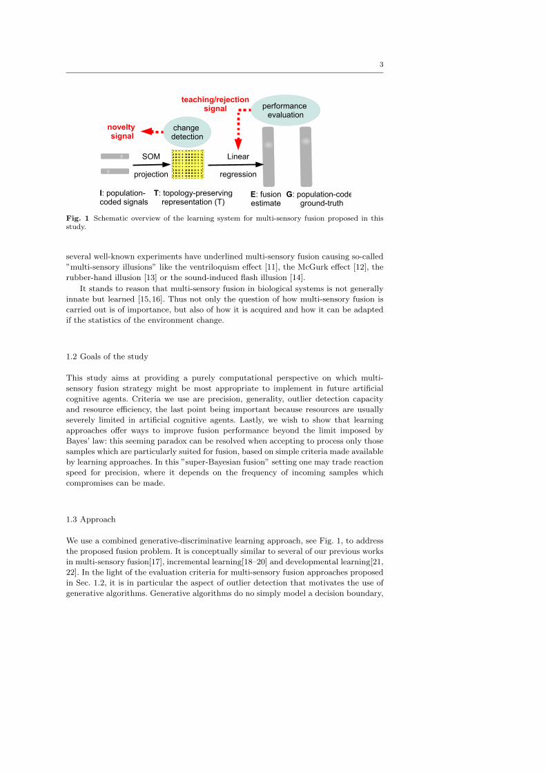
SOM
projection
Linear
regression
I: population-coded signals
T: topology-preserving representation (T)
E: fusion estimate
G: population-coded ground-truth
performance evaluation
teaching/rejection signal
change detection
novelty signal
Fig. 1 Schematic overview of the learning system for multi-sensory fusion proposed in thisstudy.
several well-known experiments have underlined multi-sensory fusion causing so-called
”multi-sensory illusions” like the ventriloquism effect [11], the McGurk effect [12], the
rubber-hand illusion [13] or the sound-induced flash illusion [14].
It stands to reason that multi-sensory fusion in biological systems is not generally
innate but learned [15,16]. Thus not only the question of how multi-sensory fusion is
carried out is of importance, but also of how it is acquired and how it can be adapted
if the statistics of the environment change.
1.2 Goals of the study
This study aims at providing a purely computational perspective on which multi-
sensory fusion strategy might be most appropriate to implement in future artificial
cognitive agents. Criteria we use are precision, generality, outlier detection capacity
and resource efficiency, the last point being important because resources are usually
severely limited in artificial cognitive agents. Lastly, we wish to show that learning
approaches offer ways to improve fusion performance beyond the limit imposed by
Bayes’ law: this seeming paradox can be resolved when accepting to process only those
samples which are particularly suited for fusion, based on simple criteria made available
by learning approaches. In this ”super-Bayesian fusion” setting one may trade reaction
speed for precision, where it depends on the frequency of incoming samples which
compromises can be made.
1.3 Approach
We use a combined generative-discriminative learning approach, see Fig. 1, to address
the proposed fusion problem. It is conceptually similar to several of our previous works
in multi-sensory fusion[17], incremental learning[18–20] and developmental learning[21,
22]. In the light of the evaluation criteria for multi-sensory fusion approaches proposed
in Sec. 1.2, it is in particular the aspect of outlier detection that motivates the use of
generative algorithms. Generative algorithms do no simply model a decision boundary,
4
e.g., for separating two classes, but attempt, in various ways, to model the entire distri-
bution of data samples in input space. This will involve, in general, a more substantial
effort, which however pays off when the objective goes beyond separating classes, as it
is the case here.
As the essential building block implementing the generative part of our model, we
chose a modified version of the self-organizing map (SOM) algorithm[23]. This is a
prototype-based generative algorithm which therefore permits the detection of outliers
and changes in input statistics. Apart from approximating the distribution of input
samples by prototype vectors, it implements a topology-preserving mapping of the
computed prototypes, which is of no direct concern here, but will become extremely
important when incremental learning is concerned [19,18]. As incremental learning is
the logical next step following successful change detection, we feel that the use of the
SOM model is very well justified in this case.
1.4 Related work
Multi-sensory fusion can be modeled in various ways, the most relevant ones being self-
organized learning and Bayesian inference. The former regroups a set of bio-inspired,
unsupervised learning algorithms while the latter argues that mammals can combine
sensory cues in a statistically optimal manner.
1.4.1 Self-organizing topology-oriented algorithms and multimodal fusion
Among artificial neural networks, self-organizing maps (SOMs) perform clustering
while preserving topological properties of the input space. Studies applying SOMs to
multimodal fusion are usually focused on reproducing properties one can find in biology:
continuous unsupervised processes, adaptation and plasticity, topological preservation
of the input space relationship, or dimensionality reduction. Self-organized approaches
have the potential to establish a transition from high-dimensional, noisy and modality-
specific sensor readings to abstract, multimodal and symbolic concepts, whereas they
are considered less appropriate for reproducing statistical optimality which should be
respected by any fusion process.
Most SOM-based approaches imitate, more or less closely, the hierarchical and
layered structure of cortical areas, especially the superior colliculus (SC). In [24] the
authors use one basic non-layered self-organizing map to simulate biological MSE and
inverse effectiveness from artificial combinations of sensory input cues with Gaussian
neighborhood and Manhattan distance. Even though their data are low-dimensional
and non-realistic, the authors confirm that the (nearly) original SOM algorithm can
lead to meaningful multisensory cue combination. As in [25], they emphasize the pos-
itive impact of a non-linear transfer function applied to map outputs (in these cases,
a sigmoid function). [26] design a SOM-like feed-forward layered architecture which
uses Hebbian learning to associate maps. The study shows how uni-sensory maps can
be aligned by a system that learns coordinate transformations, and automatically in-
tegrated into a multisensory representation, i.e. a third map. It focuses on comparing
simulated and biological responses to spatially coincident or non-coincident stimuli and
achieves the reproduction of simplistic MSE and MSD effects. [27] models the learning
of words and objects relations by young children from a psychological point of view
using two unimodal SOMs. Hebbian learning is used to model the mapping between
5
unimodal spaces so that the presentation of an object activates the correct correspond-
ing word and vice versa. [28] also deals with imitating SC multi-sensory fusion. The
study designs a SOM-based model which is task-oriented and aims at autonomously
finding a way to reach a specific goal (in this case object localization). The model tries
to characterize the reliability of sensory modalities when dealing with noisy artificial
stimuli. Using a single SOM, it uses a custom distance function that measures the like-
lihood of one input vector to be a noisy version of a known prototype. To this effect,
the original Kohonen algorithm is adapted so that the metric takes into account the
estimation of each sensor modality’s reliability. Nevertheless, noise for different modal-
ities is assumed to independent and normally distributed, and the analogy with the
superior colliculus is rather superficial.
Finally, several studies aim at designing models inspired by recent neurophysio-
logical findings without fully copying biological architectures or processes, focusing on
well-defined applications. Following [29], [30] proposes a learning algorithm based on
a variant of the original SOM, ViSOM [31], which forces the inter-unit distances in a
map to be proportional to those in the input space. As for multi-expert techniques in
supervised learning [30], a single final map is learned that takes into account multiple
SOMs. Each unit of the final map corresponds to a fusion by Euclidean distance, and
a voting process is performed on neurons at the same position of the grid in each uni-
modal SOM. Although the model does not really focus on bio-plausibility and prefers
enhancing topology preservation and data visualization properties, it is remarkable
that it allows autonomous artificial concentration on interesting features in each of the
unimodal SOMs. [32] is one of the most ambitious works using self-organized ANNs
for multi-sensory fusion without only reproducing known biological phenomena. With
a hierarchical lattice of SOMs (two unimodal maps integrated in a multimodal map),
they confirm abilities of SOMs and feedforward connections in integrating unimodal
artificial percepts into multimodal unified representations, as [33] already did. This
study above all puts forward the effective role of feedback connections in artificial at-
tentional mechanisms: without feedback, hierchical SOM networks might only achieve
multi-sensory fusion for elementary artificial stimuli. They apply their (strongly fine-
tuned) model to produce bimodal fusion of phonemes and letters but do not provide a
clear task-oriented (e.g. speech recognition) evaluation.
1.4.2 Bayesian inference as a model of multi-sensory fusion
Several psychophysiological studies have shown that mammalian brains, and in par-
ticular humans ones, fuse multiple sensory signals in an statistically optimal way by
a weighted linear combination of estimates of the individual measurements [2]. The
intrinsic uncertainty of sensory cues make them more or less reliable and this has to
be taken into account by the fusion process [34]. Most of the time, these observations
are conducted using animals at a behavioural level. However, probabilistic inference in
neural circuits is still not well understood. Among fusion methods relying on probabil-
ity distributions or density functions to express data uncertainty, Bayesian fusion is one
of the best-known techniques and is known for having strong links to biological multi-
sensory fusion [35]. It consists of weighting each sense according to its known variance
by applying maximum likelihood estimator (MLE) or maximum a posteriori (MAP)
techniques. A couple of assumptions are usually made when performing optimal fusion
according to Bayesian statistics [36–42], namely the assumption of Gaussian noise that
is applied independently to each sense, and the assumption of known variances. These
6
assumptions, while acceptable on a theoretical level, prevent the use of such techniques
in domains such as developmental learning since evidently neither the variances nor
the theoretical distribution and independence properties of signals should be known in
advance.
2 METHODS
In this section, we will give all necessary details of the used learning approach (Sec.2.4),
Bayesian inference based on estimated joint probabilities (Sec. 2.2) and model-based
Bayesian inference (Sec. 2.3). In all cases, the setting is identical: a single ”true” value
r and two noisy sensor readings s1 and s2. The way of obtaining s1 and s2 from r
depends on the particular problem that is treated, as do the noise distributions that
additionally perturb the sensor readings.
2.1 Fusion problems
Two fusion problems are considered in this study, in both of which the goal is to
infer the true value r from noisy sensor readings s1, s2. Several types of noise ε(σ)
are considered for corrupting sensor readings (Gaussian, uniform, triangular), all of
which have a single parameter σ that models their ”strength”. In the case of Gaussian
noise, σ would correspond to the standard deviation, for uniform and triangle noise
it is the half-width of the interval with nonzero probability. For every noise type in
both problems, we vary the parameter σ in order to determine how this impacts fusion
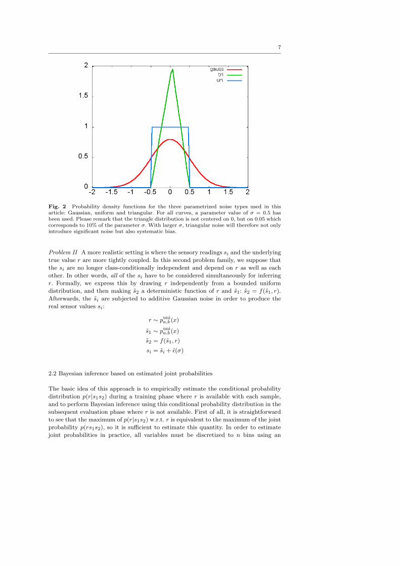
accuracy. The probability density functions for all three (additive) noise types are as
follows (see also Fig.2):
pgauss(x, σ) =1√
2πσ2exp− x2
2σ2(1)
puni(x, σ) =
{12σ if x ∈ [−σ, σ]
0 else
ptri(x, σ)
x+σ1.1σ2 iff x ∈ [−σ, 0.1σ]σ−x0.9σ2 iff x ∈ [0.1σ, σ]
0 else
Problem I This first ”family” of problems follows the ”classic” Bayesian framework:
a single ”true” value r that gives rise to several noisy sensor readings si. We suppose
that the sensor readings si are obtained from an unique r value by adding independent,
parametrized noise ε(σ).
r ∼ punia,b (x)
si = r + ε(σ)
7
Fig. 2 Probability density functions for the three parametrized noise types used in thisarticle: Gaussian, uniform and triangular. For all curves, a parameter value of σ = 0.5 hasbeen used. Please remark that the triangle distribution is not centered on 0, but on 0.05 whichcorresponds to 10% of the parameter σ. With larger σ, triangular noise will therefore not onlyintroduce significant noise but also systematic bias.
Problem II A more realistic setting is where the sensory readings si and the underlying
true value r are more tightly coupled. In this second problem family, we suppose that
the si are no longer class-conditionally independent and depend on r as well as each
other. In other words, all of the si have to be considered simultaneously for inferring
r. Formally, we express this by drawing r independently from a bounded uniform
distribution, and then making s2 a deterministic function of r and s1: s2 = f(s1, r).
Afterwards, the si are subjected to additive Gaussian noise in order to produce the
real sensor values si:
r ∼ punia,b (x)
s1 ∼ punia,b (x)
s2 = f(s1, r)
si = si + ε(σ)
2.2 Bayesian inference based on estimated joint probabilities
The basic idea of this approach is to empirically estimate the conditional probability
distribution p(r|s1s2) during a training phase where r is available with each sample,
and to perform Bayesian inference using this conditional probability distribution in the
subsequent evaluation phase where r is not available. First of all, it is straightforward
to see that the maximum of p(r|s1s2) w.r.t. r is equivalent to the maximum of the joint
probability p(rs1s2), so it is sufficient to estimate this quantity. In order to estimate
joint probabilities in practice, all variables must be discretized to n bins using an
8
invertible function bµ,n(x) → i ∈ N, where obviously a finer discretization implies
higher precision but also higher memory and execution time demands. For variables in
the [0, 1] interval, we chose b such that it pads the encoded scalar value with borders
of width µ, which is necessary because random variables might fall outside the [0, 1]
interval depending on noise, and still need to be represented properly:
b ≡ bµ,n(x) = floor (n− (µ+ (1− 2µ)x) (2)
b−1 ≡ b−1µ,n(i) =in − µ1− 2µ
(3)
For three discretized variables, the estimated joint probability matrix pijk has n3 en-
tries and requires roughly n3 samples to be filled properly. During training, samples
(r, s1, s2) are received on by one, and for each sample the matrix is updated as follows:
pijk(0) ≡ 0
pb(r)b(s1)b(s2)(t+ 1) = pb(r)b(s1)b(s2)(t) + 1 (4)
At the end of the training phase, pijk is normalized to have a sum of 1. When performing
inference during the evaluation phase, only the two sensor readings s1 and s2 are
available, and the task to infer the underlying value r∗ that best matches s1 and s2amounts to finding the matrix bin i∗ for which r has the highest estimated probability:
i∗ = maxi pi b(s1) b(s2)
r∗ = b−1(i∗) (5)
2.3 Model-based Bayesian inference
Similar in spirit to the preceding section, model-based Bayesian inference aims to find
the most probable value of r given the observations s1 and s2:
r∗ = arg maxrp(r|s1s2) ∼ arg maxrp(s1s2|r)p(r) (6)
This amounts to a maximization problem:
∂rp(s1s2|r)p(r) = 0
⇔ ∂r (p(s1s2|r)) p(r) + p(s1s2|r)∂sp(r) = 0 (7)
Eqn. (7) has trivial solutions outside the interval ]a, b[ where both p(r) and ∂sp(r)
vanish. However they minimize p(s1s2|r)p(r) (inserting an appropriate r always gives
a value of 0), and are thus excluded from our considerations. If, however, a solution
exists inside [a, b], it must obey the simplified equation
∂s (p(s1s2|r)) = 0 (8)
On the other hand, if eqn.( 8) has a non-trivial solution outside the interval ]a, b[ then
it must be either s = a or s = b, depending on which is closer, because the infinities
in the derivatives of p(r) achieve a ”clamping” of obtained fusion results to the known
interval [a, b]. This can be implemented very efficiently, without solving any equations
at all, as a post-processing step of fusion.
9
Evidently, eqn.(8) needs to be solved both for problem I and II separately, and
in general this approach requires that the data generation model be known. So, we
present two different solutions for problem I and problem II. In general, this approach
is a complex one, and the necessary analytical derivations need to be performed before
testing it. Any change in input statistics requires a repetition of these derivations,
where the form of the new statistics must be analytically.
2.3.1 Problem I
Corrupting a clean variable like r, here supposed deterministic so its distribution is
p(x|r) = δ(x − r), by additive noise drawn from one of the distributions pnoise(x, σ)
given in eqn. (1), implies the convolution of the probability densities of clean and noise
variables from which the resulting noisy variables are effectively drawn. The result of
the convolution is thus the conditional distribution p(si|r) of the form:
p(si|r) = pnoise(si − r, σ) (9)
For making the link to eqn.(8), we observe that the p(si|r) are class-conditionally
independent, and we can thus express their joint probability p(s1s2|r) by the product
of individual probabilities:
p(s1s2|r) = p(s1|r)p(s2|r)(10)
This leads to the following estimates for the underlying value r:
r∗gauss =∑i
1/σ2i∑j 1/σ2j
si (11)
r∗uni ∼ puniA,B (12)
where [A,B] = [s1 − σ1, s1 + σ1] ∩ [s2 − σ2, s2 + σ2]. For triangle noise, an analytical
treatment is difficult and is therefore omitted from these considerations.
Problem II The only tricky point consists here in computing the quantity p(s1s2|r)required by eqn. (7), which remains valid as p(r) is still uniformly distributed. Still, the
calculation is a little more cumbersome since the factorization p(s1s2|r) = Πip(si|r)no longer holds:
p(s1s2|r) =
∫ ∫ds1ds2p(s1s2|s1s2r)p(s1s2|r)
=
∫ ∫ds1ds2p(s1s2|s1s2)p(s1s2|r)
=
∫ ∫ds1ds2p(s1|s1)p(s2|s2)δ(f(r, s1)− s2)
=
∫ds1p(s1|s1)p(s2|f(s1, r)) (13)
where the first transformation follows from the law of total probability: we insert a
complete set of disjunct states s1s2. In the second line, the factor r has been removed
10
from the conditional probability p(s1s2|s1s2r) as it can be deduced from s1 and s2.
Later, the conditional probability has been split as si depends only on si.
The optimal fused value of r in the interval [a, b] is obtained as before by maximizing
eqn. (8). As the resulting expression is in general intractable analytically, we resort to
numerical methods to solve it for r, which do work well for Gaussian noise but not
for other forms of noise due to numerical problems for uniform noise and analytical
intractability for triangular noise.
2.4 Learning approach
The learning approach is schematically depicted in Fig. 1. It is essentially a three-layer
neural network that learns a set of plastic, topologically organized prototypes in its
hidden layer. A read-out mechanism between hidden and output layer maps the set of
graded prototype activities to output values using simple linear regression learning.
2.4.1 Population encoding
In order to increase the computational power of the employed algorithms (see [43]),
we adopt a population-coding approach[43] where continuous values of the input and
target variables (i.e., the noisy sensor readings s1, s2 and r) are represented by placing a
Gaussian of variance σp onto a discrete position in an one-dimensional activity vector
such that the discrete center position is in a linear relationship with the encoded
continuous value. As in Sec. 2.2, this discretization is associated with a loss of precision,
thus a sufficiently large size of the activity vector must be chosen. Furthermore, the
activity vector must have a sufficiently large margin µ around the interval to be encoded
because random variables can fall outside this interval and need to be represented as
well. The precise way of encoding a scalar value x ∈ [0, 1] into a vector v of size n is
as follows, using :
c = bµ,n(x) (14)
vi = exp− (i− c)2
2σ2p(15)
where we have used the discretizing function b from eqn.(2). As a final step in popula-
tion encoding, the vector v is normalized to have an L2 norm of 1.
2.4.2 Neural learning architecture
The architecture is essentially depicted in Fig. 1 and consists essentially of the layers
I, T and E: the input layer I obtained by concatenating two population-coded sensor
values, a hidden layer T and a fusion estimate layer E, respectively. In addition, there
is a ground-truth layer G that represents the ”true” sensor value r.
Generally, we denote neural activity vector in a 2D layer X by zX(y, t), and weight
matrices feeding layer X, represented by their line vectors attached to target position
y = (a, b), by wXy (t). For reasons of readability, we often skip the dependencies on
space and time and include them only where ambiguity would otherwise occur. Thus
we write zX instead of zX(y, t) and wX instead of wXy (t). Using this notation, the two
11
weight matrices that are subject to learning in this architecture are the connections
from I to T, wSOM and the weights from T to E, wLR.
zT (y) = wSOMy · zI (16)
zT = TFp
(zT)
(17)
zE = wLR · zT (18)
wLRy (t+ 1) = wLR
y + 2εLRzI(zE(y)− zG(y)
)(19)
wSOMy (t+ 1) = norm
(wSOMy + εSOMgσ(y − y∗)(zI − wSOM
y ))
(20)
(21)
where gs(x) is a zero-mean Gaussian function with standard deviation s and y∗ denotes
the position of the best-matching unit (the one with the highest similarity-to-input) in
P . In accordance with standard SOM training practices, the SOM learning rate and
radius, εSOM and σ, are maintained at ε0, σ0 for t < T1 and are exponentially decreased
afterwards in order to attain their long-term values ε∞, σ∞ at t = Tconv. The learning
rate of linear regression, εLR remains constant during at all times. TFp represents a
monotonous non-linear transfer function, TFp : [0, 1]→ [0, 1] which we model as follows
with the goal of maintaining the BMU value unchanged while non-linearly suppressing
smaller values:
m = maxyzT (y, t)
TFp
((zT (y)
)= mp−1
(zT (y)
)p(22)
2.4.3 Rejection strategy for super-Bayesian fusion
In this setting, we simply reject an incoming sample, i.e., take no decision, if the simple
criterion
max zE > θ (23)
with θ(t+ 1) = (1− α)θ(t) + α max zE(t). (24)
is fulfilled. Simply put, we check whether the highest activated unit in the output layer
E has an activity that is higher than the temporal average of past maximal activities,
calculated by exponential smoothing. This is pretty ad hoc and not rigorously justified,
but we find that in practice this strategy gives significant performance improvements
and in no case that we could observe deteriorates performance.
2.4.4 Novelty detection
As the hidden SOM layer implements a generative model of the sensory input, it should
be able to recognize out-of-the-ordinary samples, i.e., outliers. This is particularly im-
portant for detecting persistent changes in input statistics, which must be countered
by adapting the fusion model. Here, a change detection mechanism could provide, first
of all, a means to detect when a model should be adjusted to new realities, and further-
more to stop fusion until this has been successfully done. Such an ability is therefore
12
imperative for life-long learning in embodied agents and should be considered a sig-
nificant advantage. We approach change detection by simply monitoring the temporal
average activity of the best-matching until (BMU) in the hidden SOM layer P. This is
done because we assume that the SOM prototypes represent the joint distribution of s1and s2 in input space; any significant deviation from this distribution should therefore
result in lower input-prototype similarity which results in lower activity. Again, the
temporal average is calculated by exponential smoothing and thus requires no mem-
ory overhead. The smoothing constant β has to be set such that short-term random
fluctuations are smoothed away whereas long-term systematic changes are retained.
3 EXPERIMENTS
For all experiments, we use an interval of [0, 1] for r, s1 and s2. Each experiment is
repeated 25 times, each time with a different pairing of standard deviations which are
chosen for each sensor from the following fixed set: 0.016, 0.032, 0.048, 0.064 and 0.08.
Joint probability estimation parameters The discretization step size is set to n = 100,
and the joint probability matrix is built for n3 iterations. The margin parameter µ is
set to µ = 0.2.
Model-based Bayesian inference parameters This method is parameter-free in the sense
that it only uses the parameters contained in the data generation model. There are a
few parameters tied to the numerical solution of integrals but the standard values of
the numerical solvers always work well so it is not necessary to include them here.
Learning approach Here, several parameters need to be fixed: the hidden layer contains
15x15=225 units, the output layer has n = 100 units. The margin parameter for pop-
ulation encoding is set to µ = 0.2. The variance of Gaussians for population encoding
is fixed at σp = 3 pixels. The LR learning rate is εLR = 0.01 and the parameters for
decreasing SOM learning rate and radius are: ε0 = 0.1, σ0 = 5, ε∞ = 0.01, σ∞ = 0.5,
Tconv = 5000, T1 = 1000. The transfer function parameter p is set to 20. Total training
time is always 20.000 iterations unless otherwise mentioned, and testing is conducted
subsequently for 20.000 iterations for calculating performance statistics, with learning
turned off. The smoothing parameter for super-Bayesian fusion is α = 0.001, and the
smoothing parameter for change detection is β = 0.001 as well.
3.1 Comparison of fusion performances
In this experiment, we compare the performances of all three fusion methods (Bayesian
inference by joint probability estimation, model-based Bayesian inference and our learn-
ing approach) for problem I and problem II, each time using three noise types (Gaus-
sian, uniform and triangular noise) as described in detail in Sec. 2.1. For each method,
problem and noise type we conduct 25 separate experiments, corresponding to all pos-
sible combinations of standard deviations given above. In this way, the behavior of each
fusion method is sampled uniformly in a representative range of noise strengths in a
way that can be directly compared.
13
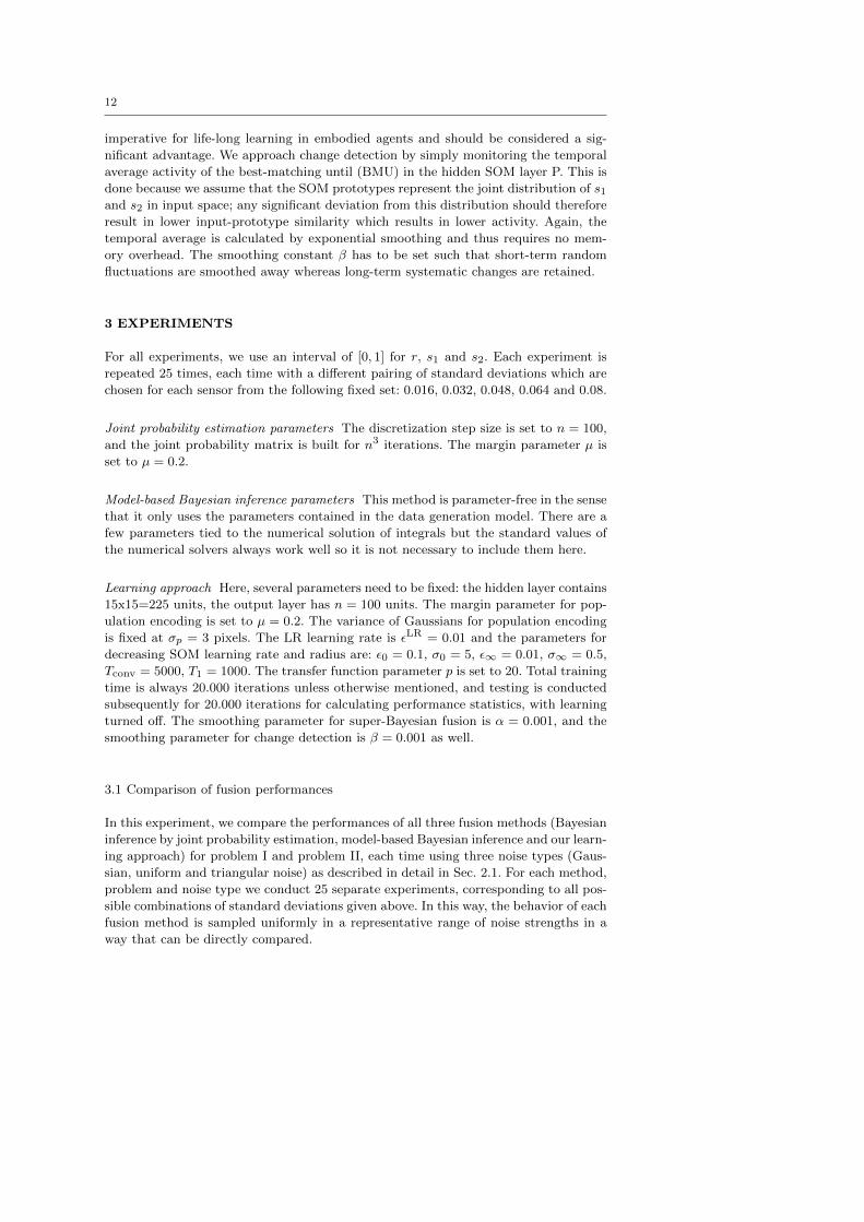
Fig. 3 Comparison of fusion performance under Gaussian noise for four methods on problemI (left) and problem II (right): Bayesian inference using estimated joint probabilities (red),model-based Bayesian inference (blue), learning approach(black) and learning approach usingsuper-Bayesian fusion(green).
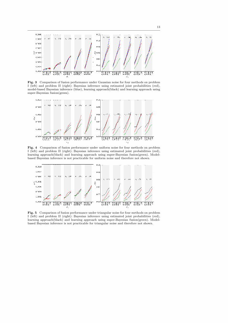
Fig. 4 Comparison of fusion performance under uniform noise for four methods on problemI (left) and problem II (right): Bayesian inference using estimated joint probabilities (red),learning approach(black) and learning approach using super-Bayesian fusion(green). Model-based Bayesian inference is not practicable for uniform noise and therefore not shown.
Fig. 5 Comparison of fusion performance under triangular noise for four methods on problemI (left) and problem II (right): Bayesian inference using estimated joint probabilities (red),learning approach(black) and learning approach using super-Bayesian fusion(green). Model-based Bayesian inference is not practicable for triangular noise and therefore not shown.
14
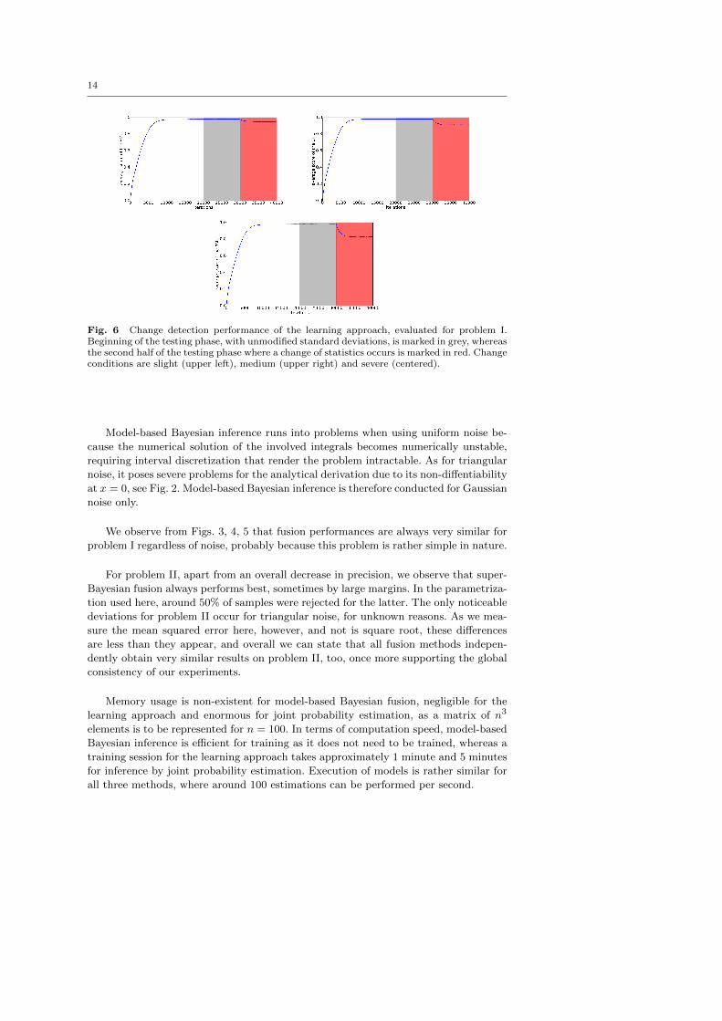
Fig. 6 Change detection performance of the learning approach, evaluated for problem I.Beginning of the testing phase, with unmodified standard deviations, is marked in grey, whereasthe second half of the testing phase where a change of statistics occurs is marked in red. Changeconditions are slight (upper left), medium (upper right) and severe (centered).
Model-based Bayesian inference runs into problems when using uniform noise be-
cause the numerical solution of the involved integrals becomes numerically unstable,
requiring interval discretization that render the problem intractable. As for triangular
noise, it poses severe problems for the analytical derivation due to its non-diffentiability
at x = 0, see Fig. 2. Model-based Bayesian inference is therefore conducted for Gaussian
noise only.
We observe from Figs. 3, 4, 5 that fusion performances are always very similar for
problem I regardless of noise, probably because this problem is rather simple in nature.
For problem II, apart from an overall decrease in precision, we observe that super-
Bayesian fusion always performs best, sometimes by large margins. In the parametriza-
tion used here, around 50% of samples were rejected for the latter. The only noticeable
deviations for problem II occur for triangular noise, for unknown reasons. As we mea-
sure the mean squared error here, however, and not is square root, these differences
are less than they appear, and overall we can state that all fusion methods indepen-
dently obtain very similar results on problem II, too, once more supporting the global
consistency of our experiments.
Memory usage is non-existent for model-based Bayesian fusion, negligible for the
learning approach and enormous for joint probability estimation, as a matrix of n3
elements is to be represented for n = 100. In terms of computation speed, model-based
Bayesian inference is efficient for training as it does not need to be trained, whereas a
training session for the learning approach takes approximately 1 minute and 5 minutes
for inference by joint probability estimation. Execution of models is rather similar for
all three methods, where around 100 estimations can be performed per second.
15
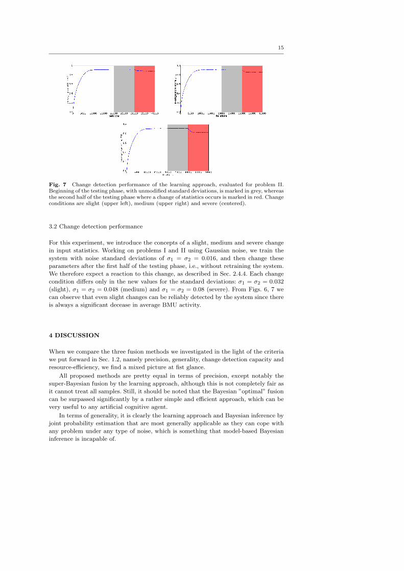
Fig. 7 Change detection performance of the learning approach, evaluated for problem II.Beginning of the testing phase, with unmodified standard deviations, is marked in grey, whereasthe second half of the testing phase where a change of statistics occurs is marked in red. Changeconditions are slight (upper left), medium (upper right) and severe (centered).
3.2 Change detection performance
For this experiment, we introduce the concepts of a slight, medium and severe change
in input statistics. Working on problems I and II using Gaussian noise, we train the
system with noise standard deviations of σ1 = σ2 = 0.016, and then change these
parameters after the first half of the testing phase, i.e., without retraining the system.
We therefore expect a reaction to this change, as described in Sec. 2.4.4. Each change
condition differs only in the new values for the standard deviations: σ1 = σ2 = 0.032
(slight), σ1 = σ2 = 0.048 (medium) and σ1 = σ2 = 0.08 (severe). From Figs. 6, 7 we
can observe that even slight changes can be reliably detected by the system since there
is always a significant decease in average BMU activity.
4 DISCUSSION
When we compare the three fusion methods we investigated in the light of the criteria
we put forward in Sec. 1.2, namely precision, generality, change detection capacity and
resource-efficiency, we find a mixed picture at fist glance.
All proposed methods are pretty equal in terms of precision, except notably the
super-Bayesian fusion by the learning approach, although this is not completely fair as
it cannot treat all samples. Still, it should be noted that the Bayesian ”optimal” fusion
can be surpassed significantly by a rather simple and efficient approach, which can be
very useful to any artificial cognitive agent.
In terms of generality, it is clearly the learning approach and Bayesian inference by
joint probability estimation that are most generally applicable as they can cope with
any problem under any type of noise, which is something that model-based Bayesian
inference is incapable of.
16
Regarding resource efficiency, especially in the light of an application in artificial
cognitive agents, it is clearly the learning approach that is most favorable: it has both
a favorable execution and training time, and it is very memory-efficient. In fact, by
reducing the size of the hidden SOM layer, one can gradually trade memory usage
for precision, making use of the graceful decay property of SOMs for this purpose.
Bayesian inference by joint probability estimation has the problem of training time and
memory usage that grow cubically with the discretization step n, quickly rendering this
approach impracticable where high precision is needed. Model-based Bayesian inference
is memory and time-efficient as well but is not very suited to artificial agents as it is
incapable of adapting.
For change detection capacity, it is the learning approach that wins the competi-
tion because it offers a very efficient-to-compute criterion to detect even rather slight
changes in input statistics, using only quantities like the BMU score that are calculated
anyway and thus do not impose a computational burden.
Based on all these points, we may safely conclude that the two adaptive approaches
to multi-sensory fusion are certainly preferable due to their generality and resource
efficiency. The learning architecture we presented possesses the additional capacity to
perform change detection and super-Bayesian fusion which are very important points
in their own right, and it rather more resource-efficient than Bayesian inference by joint
probability estimation.
4.1 Influence of key parameters on the learning approach
The most crucial parameter for the learning approach is the size of the hidden layer
T. Especially for change detection, this needs to be of sufficient size otherwise change
detection capability deteriorates significantly. Intuitively, with smaller hidden layers it
becomes harder to distinguish whether an input is dissimilar from prototypes because
it is an outlier, or because there are simply too few prototypes to properly samples the
input space. For this parameter we can say: the bigger the better: we never observed a
performance deterioration when increasing hidden layer size, but a minimum of 15x15
seems recommended for this task. Another parameter of great importance is the min-
imal neighbourhood radius σ∞. If it is set too high, neighbouring prototypes will be
too similar to each other. This means that one cannot say with surety, from each pro-
totype’s response, where exactly the input is situated, so fusion is less precise. We set
it as small as possible while still making a difference. Smaller values are acceptable as
well but do not change the behavior any more. A free parameter of moderate influence
is the transfer function parameter p = 20. It is important that there be a non-linear
stage in the network which is realized by the transfer function TFp, and results get
slightly better if p > 10. But results tend to be acceptable even for p > 1. The con-
vergence and initialization times are set w.r.t. the total number of samples according
to standard SOM practices. Learning parameters for SOM and linear regression are
similarly set w.r.t. the number of training samples.
5 Summary, conclusion and future work
We have presented a comparison of three methods for perform multi-sensory fusion in
a simulated setting that is nevertheless very closely modeled after real tasks. We com-

17
pared these methods in terms of precision, generality, change detection capacity and
resource-efficiency, and found that the self-organized neural network was most suited,
in summary, for application in artificial cognitive agents, thus making a very strong
statement in favor of learning methods in multi-sensory fusion. We furthermore inves-
tigated a simple way to improve fusion performance beyond the Bayesian optimum and
found it both practicable and beneficial for performance under the condition that one
accepts to ignore a certain percentage of incoming samples. As a last, we investigated
how fusion might be continuously updated and re-calibrated by detecting significant
changes in input statistics, and found that the detection of such changes is feasible and
simple for the presented system.
In future work, we wish to investigate the issue of incremental learning for multi-
sensory fusion, meaning that upon the detection of changed input statistics, the learned
fusion model should be adapted in a way that allows stable life-long learning. In ad-
dition, verifying these algorithms on a real-world fusion task will be an important
validation of the presented theoretical work.
6 Compliance with ethical standards
This article does not contain any studies with human participants or animals performed
by any of the authors. Thomas Hecht has received a research grant from the Direction
Generale de l’Armement (DGA), France. Alexander Gepperth, Thomas Hecht and
Mandar Gogate declare that they have no conflict of interest.
References
1. Marc O Ernst and Martin S Banks. Humans integrate visual and haptic information in astatistically optimal fashion. Nature, 415(6870):429–433, Jan 2002.
2. Dora E. Angelaki, Yong Gu, and Gregory C. DeAngelis. Multisensory integration:psychophysics, neurophysiology, and computation. Current opinion in neurobiology,19(4):452–458, 2009.
3. Marc O. Ernst and Heinrich H. Blthoff. Merging the senses into a robust percept. Trendsin cognitive sciences, 8(4):162–169, 2004.
4. Michael S. Beauchamp. See me, hear me, touch me: multisensory integration in lateraloccipital-temporal cortex. Current opinion in neurobiology, 15(2):145–153, 2005.
5. Barry E. Stein and Terrence R. Stanford. Multisensory integration: current issues fromthe perspective of the single neuron. Nature Reviews Neuroscience, 9(4):255–266, 2008.
6. Jon Driver and Toemme Noesselt. Multisensory interplay reveals crossmodal influenceson sensory-specificbrain regions, neural responses, and judgments. Neuron, 57(1):11–23,2008.
7. Mark T. Wallace. The development of multisensory processes. Cognitive Processing,5(2):69–83, 2004.
8. Gemma A. Calvert and Thomas Thesen. Multisensory integration: methodological ap-proaches and emerging principles in the human brain. Journal of Physiology-Paris,98(1):191–205, 2004.
9. Asif A. Ghazanfar and Charles E. Schroeder. Is neocortex essentially multisensory? Trendsin cognitive sciences, 10(6):278–285, 2006.
10. George M. Stratton. Vision without inversion of the retinal image. Psychological review,4(4):341, 1897.
11. Ian P. Howard and William B. Templeton. Human spatial orientation. 1966.12. Harry McGurk and John MacDonald. Hearing lips and seeing voices. 1976.13. Matthew Botvinick and Jonathan Cohen. Rubber hands’ feel’touch that eyes see. Nature,
391(6669):756–756, 1998.
18
14. Ladan Shams, Yukiyasu Kamitani, and Shinsuke Shimojo. What you see is what you hear.Nature, 2000.
15. Andrew King. Development of multisensory spatial integration. 2004.16. Monica Gori, Michela Del Viva, Giulio Sandini, and David C. Burr. Young children do
not integrate visual and haptic form information. Current Biology, 18(9):694–698, 2008.17. T Hecht and A Gepperth. A generative-discriminative learning model for noisy information
fusion. In IEEE International Conference on Development and Learning (ICDL), 2015.18. A Gepperth and M Lefort. Biologically inspired incremental learning for high-dimensional
spaces. In IEEE International Conference on Development and Learning (ICDL), 2015.19. A Gepperth and C Karaoguz. A bio-inspired incremental learning architecture for applied
perceptual problems. Cognitive Computation, 2015. accepted.20. A Gepperth, M Lefort, T Hecht, and U Korner. Resource-efficient incremental learning
in high dimensions. In European Symposium On Artificial Neural Networks (ESANN),2015.
21. M Lefort and A Gepperth. Active learning of local predictable representations with artifi-cial curiosity. In IEEE International Conference on Development and Learning (ICDL),2015.
22. A Gepperth. Efficient online bootstrapping of representations. Neural Networks, 2012.23. Teuvo Kohonen. Essentials of the self-organizing map. Neural Networks, 37:52–65, 2013.24. Jacob G. Martin, M. Alex Meredith, and Khurshid Ahmad. Modeling multisensory en-
hancement with self-organizing maps. Frontiers in computational neuroscience, 3, 2009.25. Thomas J. Anastasio and Paul E. Patton. A two-stage unsupervised learning algorithm re-
produces multisensory enhancement in a neural network model of the corticotectal system.The Journal of neuroscience, 23(17):6713–6727, 2003.
26. Athanasios Pavlou and Matthew Casey. Simulating the effects of cortical feedback inthe superior colliculus with topographic maps. In Neural Networks (IJCNN), The 2010International Joint Conference on, pages 1–8. IEEE, 2010.
27. Julien Mayor and Kim Plunkett. A neurocomputational account of taxonomic respondingand fast mapping in early word learning. Psychological review, 117(1):1, 2010.
28. Johannes Bauer, Cornelius Weber, and Stefan Wermter. A som-based model for multi-sensory integration in the superior colliculus. In Neural Networks (IJCNN), The 2012International Joint Conference on, pages 1–8. IEEE, 2012.
29. Apostolos Georgakis, Haibo Li, and Mihaela Gordan. An ensemble of SOM networks fordocument organization and retrieval. In Int. Conf. on Adaptive Knowledge Representationand Reasoning (AKRR05), page 6, 2005.
30. Bruno Baruque and Emilio Corchado. A bio-inspired fusion method for data visualization.In Hybrid Artificial Intelligence Systems, pages 501–509. Springer, 2010.
31. Hujun Yin. ViSOM-a novel method for multivariate data projection and structure visual-ization. Neural Networks, IEEE Transactions on, 13(1):237–243, 2002.
32. Tamas Jantvik, Lennart Gustafsson, and Andrew P. Papliski. A self-organized artificialneural network architecture for sensory integration with applications to letter-phonemeintegration. Neural computation, 23(8):2101–2139, 2011.
33. Valentina Gliozzi, Julien Mayor, Jon-Fan Hu, and Kim Plunkett. The impact of labels onvisual categorisation: A neural network model. 2008.
34. Michael S. Landy, Martin S. Banks, and David C. Knill. Ideal-observer models of cueintegration. Sensory cue integration, pages 5–29, 2011.
35. David C. Knill and Alexandre Pouget. The bayesian brain: the role of uncertainty inneural coding and computation. TRENDS in Neurosciences, 27(12):712–719, 2004.
36. Robert A. Jacobs. Optimal integration of texture and motion cues to depth. Visionresearch, 39(21):3621–3629, 1999.
37. Peter W. Battaglia, Robert A. Jacobs, and Richard N. Aslin. Bayesian integration ofvisual and auditory signals for spatial localization. JOSA A, 20(7):1391–1397, 2003.
38. Marc O. Ernst. A bayesian view on multimodal cue integration. Human body perceptionfrom the inside out, pages 105–131, 2006.
39. Hannah B. Helbig and Marc O. Ernst. Optimal integration of shape information fromvision and touch. Experimental Brain Research, 179(4):595–606, 2007.
40. Mustapha Makkook, Otman Basir, and Fakhreddine Karray. A reliability guided sensorfusion model for optimal weighting in multimodal systems. In Acoustics, Speech and SignalProcessing, 2008. ICASSP 2008. IEEE International Conference on, pages 2453–2456.IEEE, 2008.

19
41. Xuan Song, Jinshi Cui, Huijing Zhao, and Hongbin Zha. Bayesian fusion of laser andvision for multiple people detection and tracking. In SICE Annual Conference, 2008,pages 3014–3019. IEEE, 2008.
42. Lasse Klingbeil, Richard Reiner, Michailas Romanovas, Martin Traechtler, and YiannosManoli. Multi-modal sensor data and information fusion for localization in indoor envi-ronments. In Positioning Navigation and Communication (WPNC), 2010 7th Workshopon, pages 187–192. IEEE, 2010.
43. A Gepperth, B Dittes, and M Garcia Ortiz. The contribution of context information: acase study of object recognition in an intelligent car. Neurocomputing, 2012.
Related Documents