A generalized solution for transient radial flow in hierarchical multifractal fractured aquifers

$Page 1: A generalized solution for transient radial flow in hierarchical multifractal fractured aquifers$
A generalized solution for transient radial flow

in hierarchical multifractal fractured aquifers

Gerard Lods1 and Philippe Gouze1

Received 30 April 2008; revised 3 September 2008; accepted 17 September 2008; published 5 December 2008.

[1] An analytical solution in the Laplace domain is derived for modeling anomalouspressure diffusion during pumping tests in aquifer displaying hierarchical fractalfracture networks. The proposed solution generalizes all of the analytical models forfractal flow published previously by combining multifractal diffusion and nestedmultiporosity with transient exchanges, interface skin effects, and well storage effect.Solutions are derived for fracture-delimited blocks with planar, cylindrical, and sphericalshapes, as well as with any fractional dimensional shapes. Any combinations of theseshapes can be defined in order to model a large range of situations. Within eachpermeability level, the fractal properties of the fracture network can be specified and thefractal dimension can be distinct from the shape dimension of the block.

Citation: Lods, G., and P. Gouze (2008), A generalized solution for transient radial flow in hierarchical multifractal fractured

aquifers, Water Resour. Res., 44, W12405, doi:10.1029/2008WR007125.

1. Introduction

[2] Hydraulic properties of reservoirs are usually inferredfrom well tests (either pumping or injection tests) by fittingthe parameters of heuristic models that account for theassumed hydrodynamic features (e.g., heterogeneity) ofthe medium. For instance, fractured reservoirs often displaydistinct sets of conductive fractures which may beconnected to each other, and which usually delimit lessconductive zones. In their pioneering work, Barenblatt et al.[1960] introduced the double-porosity concept, proposingthat reservoirs can be represented by two overlappingcontinua with distinctly different porosity values. Theydistinguished a main fracture network, where flow takesplace at the scale of the volume affected by the pumpingtest, and porous blocks that can be drained by the fractures.Mass transfers between fractures and blocks can be modeledeither by stationary [Warren and Root, 1963] or transient[Boulton and Streltsova, 1977] formulations. Stationaryexchange models assume instantaneous diffusion in theblocks, while the mass exchange rate is controlled bythe difference in head between the fracture and the block.The transient exchange approach is much more realistic, andhas been improved by parameterization of the fracture skineffect [Moench, 1984] that allows modeling of the expectedhydraulic impedance at the fracture-block interface due tothe presence of pre-existing mineral deposits or an alterationlayer. The introduction of the skin effect unifies the twotypes of exchange, since fracture-block exchange tends tobe stationary if fracture-block impedance is high.[3] Several models have been proposed to account for

more complex reservoir properties and specific shapes ofthe drawdown or recovery curves derived from pumping

tests. The triple-porosity model was introduced by Closman[1975], and further developed by Abdassah and Ershaghi[1986], who proposed analytical solutions to model flow ina fractured network exchanging water (transient) with twomatrix continua displaying distinct hydrodynamic proper-ties. Rodriguez et al. [2004] proposed analytical solutionswith stationary exchanges between two nested sets offractures and a porous matrix. Pulido et al. [2006] addressedsolutions for modeling transient exchanges, including theskin effect, between a fracture network, a microfracturenetwork and a porous matrix assuming that microfracturesare unconnected on a large scale.[4] The presence of vugular cavities in reservoirs has also

been investigated. Liu et al. [2003] proposed analyticalsolutions with stationary exchange between a fracturenetwork, vugular cavities and matrix blocks, assuming thatvugular cavities are unconnected at the large scale (i.e.,fractures segregate both the matrix and the vugular cavities).This model was extended to the possible large-scale con-nectivity of vugular cavities (i.e., vugular cavities areconnected to the well) by Camacho-Velazquez et al.[2005], while Pulido et al. [2007] gave solutions accountingfor transient exchanges and skin effect between fractures,vugular cavities and matrix.[5] A more general multicontinuum approach was pro-

posed by Bai et al. [1993]. However, although multicontin-uum models may be appropriate for studying fluid flow insystems with hierarchized permeability, they do not accountfor the fractal properties of fracture networks as commonlyobserved in natural reservoirs [Le Borgne et al., 2004;Bernard et al., 2006]. For example, the models listed abovedo not account for (1) the scale dependence of porosity andpermeability and (2) the nonuniform connectivity distribu-tion of fracture networks and the presence of critical linksacting as bottlenecks that may generate anomalous diffusion[see de Dreuzy and Davy, 2007, and references herein].[6] Fractal properties of fractured reservoirs have been

studied intensively following the pioneering developments

1Laboratoire Geosciences, Universite Montpellier 2 - CNRS, Montpel-lier, France.

Copyright 2008 by the American Geophysical Union.0043-1397/08/2008WR007125

W12405

WATER RESOURCES RESEARCH, VOL. 44, W12405, doi:10.1029/2008WR007125, 2008

1 of 17

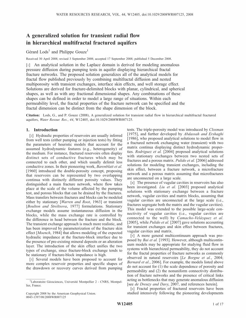
byMandelbrot [1983]. Fragmentation processes were relatedto fractal properties by Turcotte [1986], and numerous fieldmeasurements have shown that natural fracture networkspossess fractal properties [e.g., Barton and Hsieh, 1989;Nolte et al., 1989; Chelidze and Gueguen, 1990; Sahimi etal., 1993]. The calculation of radial diffusion in syntheticfractal networks has revealed some specific features, such aspower law scaling of porosity and conductivity with the radialdistance from the source, which leads to anomalous diffusion[O’Shaughnessy and Procaccia, 1985]. For example,Figure 1 shows a fractal two-dimensional network withporosity and conductivity scaling according to a power lawwith the radial distance to the centre. The fractal distributionhas porosity and conductivity power law exponents of�0.22and �0.29, respectively, while the exponents are nil in thecase of a uniform network occupying the whole grid.[7] Barker [1988] has proposed analytical solutions for

modeling pumping tests without anomalous diffusion in asingle-porosity system, but characterized by a fractionalflow dimension. This model generalizes the Euclideandimension to nonintegral flow dimensions that accountsfor the fractal structure of the fracture network. The value offlow dimension is unity for a parallel flow, such as flow in avertical fault intercepted by the pumping well. Flow dimen-sion is 2 for cylindrical flow in a pumping test, for example,when the well completely penetrates a homogeneous porousaquifer; this is the underlying assumption of Theis’s model[Theis, 1935]. Flow dimension is 3 for spherical flow asexpected in the case of pumping concentrated within asingle fracture (using a dual packer system) connected toa dense and extended network. Note however that the fractalscale dependence is restricted to identical exponents forporosity and conductivity power law in the Barker’s model[Walker and Roberts, 2003]. Barker’s model has beenextended by Hamm and Bidaux [1996] to double-porositysystems with transient exchanges including fracture skinparameterization. Models with a fractional flow dimensionhave proved useful in cases where integral dimensionsolutions are not satisfactory [Lods and Gouze, 2004], butthey do not account for anomalous diffusion. Analyticalsolutions for anomalous diffusion have been put forward byChang and Yortsos [1990], generalizing the single-porositymodel of Barker [1988].[8] The aim of the present study is to provide analytical

solutions for modeling anomalous pressure diffusion during

pumping tests in aquifer displaying hierarchical fractalfractures sets. The proposed solutions generalize all themodels presented above (see Table 1). We consider a mainfracture network intercepted by the pumping well. Thisfracture network delimits blocks in which fractal diffusionis controlled by fractures at a lower level (Figure 2). Thishierarchy is implemented recursively, which eventuallyleads to a hierarchical fractal permeability system (or multi-fractal system). Each of the fracture levels exchanges waterwith the blocks that are delimited in this way. Exchanges aretransient and take into account possible skin effects.Solutions are derived for a block shape of dimension 1for planar blocks, 2 for cylindrical blocks, and 3 forspherical blocks [Boulton and Streltsova, 1977; Moench,1984; Barker, 1985a, 1985b], as well as for any fractionaldimension. Any combination of these shapes is allowed.Within each permeability level, the fractal properties of thefracture network can be specified and the fractal dimensioncan be different from the shape dimension of the block.[9] In addition to the skin effect that may occur at the

fracture-block interfaces, our model also takes account ofthe wellbore skin effect [van Everdingen, 1953]. This effectis known to be potentially important, and is modeled here asa singular head loss or gain at the well-reservoir interface. Apositive skin effect factor is used to model laminar andturbulent head losses occurring in the well, in the equipment(e.g., slotted tubing, gravel pack) or in close proximity tothe well due to eventual damage during drilling operations(e.g., rock alteration or mud invasion). On the contrary,negative skin factors must be used to account for theincrease in conductivity observed after well developmentor when the aperture of the fractures intersecting the well islarge in the vicinity of the well.[10] In addition, our model includes a parameterization of

the well storage effect [Papadopulos and Cooper, 1967]due to the difference in storage and conductivity betweenthe well and the reservoir. Well storage effects are particu-larly important for large-diameter wells and when the rock

Figure 1. Synthetic two-dimensional networks withporosity and conductivity power law radial scaling,modified from the work of Acuna and Yortsos [1995].(a) Uniform regular network; scaling exponents are 0.(b) Fractal distribution; negative, distinct scaling exponentsof porosity and conductivity.

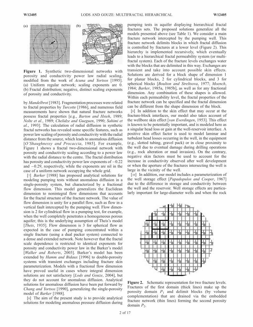
Figure 2. Schematic representation for two fracture levels.Fractures of the first domain (thick lines) make up theporosity domain P1 and delimit blocks (by volumecomplementation) that are drained via the embeddedfracture network (thin lines) forming the second porositydomain P2.

2 of 17

W12405 LODS AND GOUZE: MULTIFRACTAL HIERARCHICAL W12405

formation conductivity is low. Note that this effect cannotbe taken into account in models assuming an infinitesimalsource, such as in Theis’s model.[11] In the next section, we present the governing equa-

tions and solutions in the Laplace domain (the full mathe-matical treatments are given in Appendix A). Theapplication and parameterization of the model is discussedand illustrated in section 3, along with examples of increas-ing complexity as well as a parameter sensitivity analysis.Section 4 provides some concluding remarks emphasizingthe improvements and some limitations of the model.

2. Governing Equations

[12] In the following, we assume a confined isotropicaquifer, radially infinite and initially at rest. Flow occurs ina hierarchical fractured system containing m levels offractures. The first fracture network level is fully connectedwithin the entire domain, and consequently to the pumpingwell. This fracture network forms the porosity domain P1

and delimits blocks defined by volume complementation.The blocks within P1 are fractured by fractures that form theporosity domain P2. The porosity domain P2 is not fullyconnected since it is segregated by the fractures forming theporosity domain P1, but the properties of P2 are assumed tobe statistically identical in each of the blocks. The samehierarchical organization is applied recursively for i = 2, . . .,m � 2, where porosity domain Pi is made up of fracturesdelimiting blocks that are drained peripherally. These blocksare affected by fractures forming the fracture network oflevel i + 1 (i.e., the porosity domain Pi + 1). The porositydomain Pm�1 delimits the smallest permeable blocks (theporosity domain Pm) and drains them peripherally. The

properties are assumed statistically identical in each of thesegregated blocks embedding the porosity domain Pi for 2 <i � m. By convention, the blocks embedding domain Pi arereferred to in the following as Pi blocks.[13] To account for fractal flow, Acuna and Yortsos

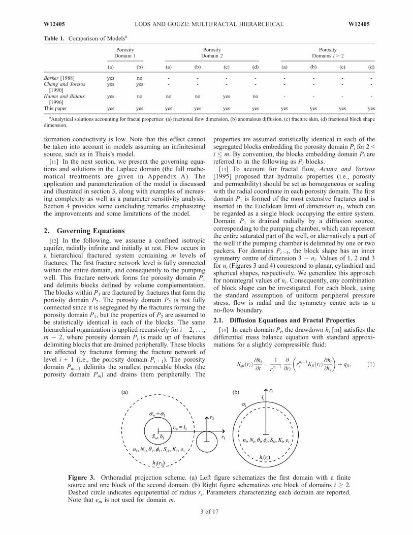
[1995] proposed that hydraulic properties (i.e., porosityand permeability) should be set as homogeneous or scalingwith the radial coordinate in each porosity domain. The firstdomain P1 is formed of the most extensive fractures and isinserted in the Euclidean limit of dimension n1, which canbe regarded as a single block occupying the entire system.Domain P1 is drained radially by a diffusion source,corresponding to the pumping chamber, which can representthe entire saturated part of the well, or alternatively a part ofthe well if the pumping chamber is delimited by one or twopackers. For domains Pi >1, the block shape has an innersymmetry centre of dimension 3 � ni. Values of 1, 2 and 3for ni (Figures 3 and 4) correspond to planar, cylindrical andspherical shapes, respectively. We generalize this approachfor nonintegral values of ni. Consequently, any combinationof block shape can be investigated. For each block, usingthe standard assumption of uniform peripheral pressurestress, flow is radial and the symmetry centre acts as ano-flow boundary.

2.1. Diffusion Equations and Fractal Properties

[14] In each domain Pi, the drawdown hi [m] satisfies thedifferential mass balance equation with standard approxi-mations for a slightly compressible fluid:

Ssfi rið Þ @hi@t

¼ 1

rni�1i

@

@rirni�1i Kfi rið Þ @hi

@ri

� �þ qfi; ð1Þ

Table 1. Comparison of Modelsa

PorosityDomain 1

PorosityDomain 2

PorosityDomains i > 2

(a) (b) (a) (b) (c) (d) (a) (b) (c) (d)

Barker [1988] yes no - - - - - - - -Chang and Yortsos[1990]

yes yes - - - - - - - -

Hamm and Bidaux[1996]

yes no no no yes no - - - -

This paper yes yes yes yes yes yes yes yes yes yes

aAnalytical solutions accounting for fractal properties: (a) fractional flow dimension, (b) anomalous diffusion, (c) fracture skin, (d) fractional block shapedimension.

Figure 3. Orthoradial projection scheme. (a) Left figure schematizes the first domain with a finitesource and one block of the second domain. (b) Right figure schematizes one block of domains i � 2.Dashed circle indicates equipotential of radius ri. Parameters characterizing each domain are reported.Note that em is not used for domain m.

W12405 LODS AND GOUZE: MULTIFRACTAL HIERARCHICAL

3 of 17

W12405

where ri [m] is the radial Euclidean distance from the sourcecentre for Pi = 1, and the radial Euclidean distance from thecentre of the embedding blocks for the other domains Pi > 1

(Figure 3), t [s] is the elapsed time, Ssfi [m�1] is the specific

storage, Kfi [m s�1] is the hydraulic conductivity and qfi[s�1] is the exchange flow rate density between Pi and Pi + 1.By construction, qfm = 0. Following the approach by Acunaand Yortsos [1995], we can define the fractal scaled values(denoted by f subscript) for specific storage Ssfi and hydraulicconductivity Kfi as follows:

Kfi rið Þ ¼ KirNi�ni�qii ; ð2Þ

and:

Ssfi rið Þ ¼ SsirNi�nii ; ð3Þ

where Ssi and Ki are the values of the specific storage and thehydraulic conductivity on the unit radius hypersphere.Similarly, this scaling can be applied for porosity:

ffi rið Þ ¼ firNi�nii ð4Þ

where fi is the porosity value on the unit-radius hypersphere.In this study, we implement the standard relations (as used inpetroleum engineering, for example) between Ssi, Ki and fi:Ssi = �rfici and Ki = �rfiki/m, where �r [kg m�2 s�2] denotesthe product of the fluid density and the gravity acceleration,m [m�1 s�1 kg] is the dynamic viscosity of the fluid, ci [m s2

kg�1] is the total compressibility and ki [m2+qi] is the fractal

permeability. In equations (2) to (4), Ni is the (fractal)density dimension of the fracture network (Ni � ni) and qi isthe anomalous diffusion exponent (qi � 0). Anomalousdiffusion arises, for example, from null-aperture distributedzones in individual fractures or from pore-space connectiv-ity of the fracture network [de Dreuzy and Davy, 2007]. Theanomalous diffusion exponent is related to the random walkdimension q0i on a fractal lattice, by qi = 2 � q0i [Havlin andBen-Avraham, 1987]. Conversely, the fractal densitydimension Ni is related to the spectral dimension N0

i (1 �N0

i � Ni), which corresponds to the flow dimension ofBarker’s model [Barker, 1988]:

N 0i ¼ 2Ni= 2þ qið Þ: ð5Þ

Initial and boundary conditions are defined by:

hi t ¼ 0ð Þ ¼ 0; ð6Þ

limr1!1

h1 ¼ 0; ð7Þ

and

limri!0

Kfi

@hi@ri

� �¼ 0; i > 1: ð8Þ

2.2. Exchange Terms

[15] The exchange flow rate density qfi is the product ofthe exchange area density and the local velocity. Assumingthat the hydraulic conductivities of domain Pi and Pi+1 aredistinctly different, the local velocity is controlled by theconductivity value of the less conductive porosity domain.Then, taking Kf i+1 < Kfi by construction, we obtain theexchange flow rate density, qfi, for porosity domains Pi<m:

qfi ¼ �cfiþ1 Kfiþ1

@hiþ1

@riþ1

� �riþ1¼liþ1

; ð9Þ

where cfi+1 [m�1] is the exchange area density, and li+1 is

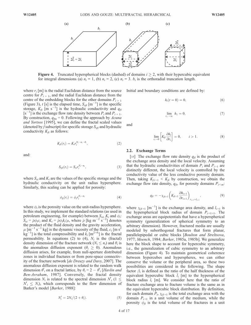
the hyperspherical block radius of domain Pi+1>1. Theexchange areas are equipotentials that have a hypersphericalsymmetry (generalization of spherical symmetry to anarbitrary dimension). However, fractured media are usuallymodeled by suborthogonal fractures that form planar,parallelepipedal or cubic blocks [Boulton and Streltsova,1977; Moench, 1984; Barker, 1985a, 1985b]. We generalizehere the block shape to account for hypercubic symmetry,i.e., the generalization of cubic symmetry to an arbitrarydimension (Figure 4). To maintain geometrical coherencebetween hypercubes and hyperspheres, we can eitherconserve the volume or the peripheral area, so these twopossibilities are considered in the following. The shapefactor bi is defined as the ratio of the half thickness of theequivalent hypercubic block �li [m] to the hypersphericalblock radius li [m]. We consider here that the ratio offracture exchange area to fracture volume is the same as inthe equivalent hypercubic block distribution. By definition,for each domain Pi, cfi+1 is the total exchange area with thedomain Pi+1 in a unit volume of the medium, while theporosity ffi is the total volume of the fractures in a unit

Figure 4. Truncated hyperspherical blocks (dashed) of domains i � 2, with their hypercubic equivalentfor integral dimensions (a) ni = 1, (b) ni = 2, (c) ni = 3. bi is the orthoradial truncation length.

4 of 17


volume of the medium. Consequently, the ratio of fractureexchange area to fracture volume can be written as:

cfiþ1

ffi rið Þ ¼Liþ1

1�Diþ1

; ð10Þ

where Li [m�1] andDi [�] denote the exchange area density

and the volume density, respectively, of the Pi blocks for anhypercubic block distribution. Li+1/(1 � Di+1) is theexchange area between domains Pi and Pi+1 divided by thefracture volume of domain Pi. This relation is valid because,by volumetric complementation, 1 � Di+1 is the fracturevolume density of Pi.[16] The exchange area density cfi+1 defined by equation

(10) scales radially, as expected for an area embedding afractal volume that scales with the radial distance. Thisscaling of the exchange area density with the exponent ofthe porosity is in agreement with the findings by Delay et al.[2007], who observed a similar scaling property of theexchange coefficient with porosity. Their results were basedon the analysis of pumping tests using a fractal double-porosity model with stationary exchange. This scalingaccounts for the fact that, when porosity of domain Pi

decreases, the exchange area density decreases because ofthe radius increase of the Pi+1 block.[17] The calculation of bi, Li and Di is given in Table 2.

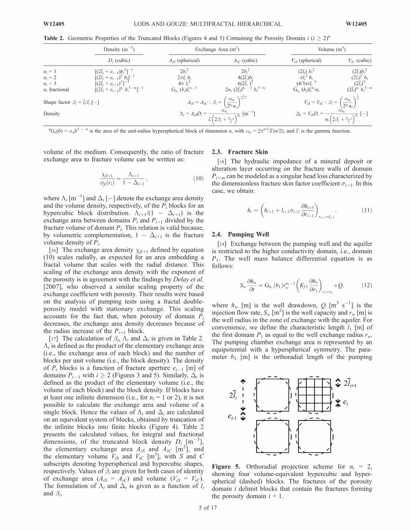
Li is defined as the product of the elementary exchange area(i.e., the exchange area of each block) and the number ofblocks per unit volume (i.e., the block density). The densityof Pi blocks is a function of fracture aperture ei�1 [m] ofdomains Pi�1 with i � 2 (Figures 3 and 5). Similarly, Di isdefined as the product of the elementary volume (i.e., thevolume of each block) and the block density. If blocks haveat least one infinite dimension (i.e., for ni = 1 or 2), it is notpossible to calculate the exchange area and volume of asingle block. Hence the values of Li and Di are calculatedon an equivalent system of blocks, obtained by truncation ofthe infinite blocks into finite blocks (Figure 4). Table 2presents the calculated values, for integral and fractionaldimensions, of the truncated block density Di [m�3],the elementary exchange area AiS and AiC [m2], andthe elementary volume ViS and ViC [m3], with S and Csubscripts denoting hyperspherical and hypercubic shapes,respectively. Values of bi are given for both cases of identityof exchange area (AiS = AiC) and volume (ViS = ViC).The formulation of Li and Di is given as a function of liand bi.

2.3. Fracture Skin

[18] The hydraulic impedance of a mineral deposit oralteration layer occurring on the fracture walls of domainPi<m can be modeled as a singular head loss characterized bythe dimensionless fracture skin factor coefficient si+1. In thiscase, we obtain:

hi ¼ hiþ1 þ liþ1siþ1

@hiþ1

@riþ1

� �riþ1¼liþ1

: ð11Þ

2.4. Pumping Well

[19] Exchange between the pumping well and the aquiferis restricted to the higher conductivity domain, i.e., domainP1. The well mass balance differential equation is asfollows:

Sw@hw@t

¼ Gn1 b1ð Þrn1�1w Kf 1

@h1@r1

� �r1¼rw

þQ; ð12Þ

where hw [m] is the well drawdown, Q [m3 s�1] is theinjection flow rate, Sw [m2] is the well capacity and rw [m] isthe well radius in the zone of exchange with the aquifer. Forconvenience, we define the characteristic length l1 [m] ofthe first domain P1 as equal to the well exchange radius rw.The pumping chamber exchange area is represented by anequipotential with a hyperspherical symmetry. The para-meter b1 [m] is the orthoradial length of the pumping

Table 2. Geometric Properties of the Truncated Blocks (Figures 4 and 5) Containing the Porosity Domain i (i � 2)a

Density (m�3) Exchange Area (m2) Volume (m3)

Di (cubic) AiS (spherical) AiC (cubic) ViS (spherical) ViC (cubic)

ni = 1 [(2�li + ei�1)bi2]�1 2bi

2 2bi2 (2li) bi

2 (2�li)bi2

ni = 2 [(2�li + ei�1)2 bi]

�1 2pli bi 4(2�li)bi pli2 bi (2�li)

2 bini = 3 [(2�li + ei�1)

3]�1 4p li2 6(2�li )

2 (4/3)pli3 (2�li)

3

ni fractional [(2�li + ei�1)ni bi

3�ni]�1 Gni(bi)li

ni�1 2ni (2�lI)ni �1 bi

3�ni Gni(bi)li

ni/ni (2�lI)ni bi

3�ni

Shape factor bi = �li/li [�] AiS = AiC : bi =ani

2ni ni

� � 1ni�1

ViS = ViC : bi =ani

2ni ni

� � 1ni

Density Li = AiSDi =ani

li 2bi þ ei�1

li

� �ni [m�1] Di = ViSDi =ani

ni 2bi þ ei�1

li

� �ni [�]

aGn(b) = anb3 � n is the area of the unit-radius hyperspherical block of dimension n, with an = 2pn/2/G(n/2), and G is the gamma function.

Figure 5. Orthoradial projection scheme for ni = 2,showing four volume-equivalent hypercubic and hyper-spherical (dashed) blocks. The fractures of the porositydomain i delimit blocks that contain the fractures formingthe porosity domain i + 1.


5 of 17

W12405

chamber, that is to say, the conductive thickness indimension 2. Gn1

(b1) is the area of a unit-radius hyper-spherical pumping chamber of dimension n1 and orthoradiallength b1 (see Table 2). The well-skin effect is representedby a singular head loss, using the dimensionless well skinfactor sw, which is also denoted as s1 for convenience. Theformulation is similar to equation (11) and can be written as:

hw ¼ h1 � rwsw

@h1@r1

� �r1¼rw

: ð13Þ

If a nonlinear skin effect occurs due to turbulent flow, thevalue of the skin factor increases with the flow rate. Weintroduce a value for critical flow rate Qc [m

3 s�1; Qc > 0],delimiting laminar and turbulent flow, such that the Qderivative of sw is continuous [Lods and Gouze, 2004]:

sw ¼ sw‘ þ swtH Qj j � Qcð Þ Qj j � Qcð Þpw= Qj j; ð14Þ

where sw‘ [�] and swt [m3(1 � pw) spw�1] are the linear

(laminar) and nonlinear (turbulent) skin factor coefficients,respectively, setting swt > 0, while pw [�] is the nonlinearhead loss exponent [Rorabaugh, 1953], with pw > 1, and His the Heaviside function. The initial condition is definedby:

hw t ¼ 0ð Þ ¼ 0: ð15Þ

2.5. Scaling Law Substitution

[20] By substituting the scaling laws (equations (2) to (4))in equations (1), (9), (10), and (12), we obtain diffusionequations having the same constant parameters as thosedefined on the unit-radius hypersphere:

Ssi@hi@t

¼ 1

rNi�1i

@

@rirNi�1�qii Ki

@hi@ri

� �þ qi; ð16Þ

qm ¼ 0; ð17Þ

qi ¼ �ciþ1lNiþ1�niþ1�qiþ1

iþ1 Kiþ1

@hiþ1

@riþ1

� �riþ1¼liþ1

; i < m; ð18Þ

ciþ1 ¼fiLiþ1

1�Diþ1

; i < m; ð19Þ

Sw@hw@t

¼ Gn1 b1ð ÞrN1�1�q1w K1

@h1@r1

� �r1¼rw

þQ: ð20Þ

The transformation of equations (1), (9), (10), and (12) toequations (16)–(20) eliminates the radial scaling of storageand exchange area, while changing the diffusion dimension-ality, and cancels the infinite-porosity inconsistency at thecentre of the blocks (see section 3.4.1). Equation (16) is thestandard diffusion equation in a space of dimension Ni withuniform specific storage Ssi. However, the hydraulicconductivity is scaled by Kiri

�qi, so the diffusivity Kiri�qi/Ssi

is scaled accordingly. In the case of anomalous diffusion, thehydraulic conductivity tends to infinity at the centre of theblocks, but the no-flow boundary condition (8) maintains afinite flux. The exchange area density (19) can be rewritten asfollows by using Li+1 = Di+1ni+1/li+1:

ciþ1 ¼ tiLiþ1 ¼ ti � fið Þniþ1=liþ1; i < m; ð21Þ

where ti is the effective fracture volume ratio, i.e., theratio of porosity subject to diffusion to the fracture volumebounded by the complementary block distribution:

ti ¼ fi= 1�Diþ1ð Þ; i < m: ð22Þ

A value of ti = 1 corresponds to a fully accessible fracturevolume, while a value of fi < ti < 1 is used to model theexistence of a nonaccessible fraction of the fracturevolume (e.g., precipitation features or fracture filling).

2.6. Analytical Solutions

[21] In the Laplace domain, we obtain the followingsolutions for ~hw, the drawdown in the well, and ~h1, thedrawdown at any location in domain P1:

~hw ¼ Q

p

Kn1 g1lE1

1

� �þ swg1E1l

E1

1 Kn1�1 g1lE1

1

� �pSwKn1 g1l

E1

1

� �þ g1E1 Gn1 b1ð ÞK1l

N1�E1

1 þ pSwswlE1

1

� �Kn1�1 g1l

E1

1

� �

and

~h1 ¼Q

p

rn1E1

1 Kn1 g1rE1

1

� �pSwl

n1E1

1 Kn1 g1lE1

1

� �þ g1E1 Gn1 b1ð ÞK1l

N1=21 þ pSwswl

n1E1þE1

1

� �Kn1�1 g1l

E1

1

� � ;

where p is the Laplace variable and K is the modified Besselfunction of the second kind. In equations (23) and (24) andlater in equation (31) auxiliary variables are defined by:

Ei ¼ 2þ qið Þ=2 ¼ q0i=2; ð25Þ

ni ¼ 1� Ni=2Ei ¼ 1� N 0i =2 ð26Þ

gm ¼ffiffiffiffiffiffiffiffiffiffip=xm

p=Em; ð27Þ

gi ¼

ffiffiffiffiffiffiffiffiffiffiffiffiffiffiffiffiffiffiffiffiffiffiffiffiffiffiffiffiffiffiffiffiffiffiffiffiffiffiffiffiffiffiffiffiffiffiffiffiffiffiffiffiffiffiffiffiffiffiffiffiffiffiffiffiffiffiffiffiffiffiffiffiffiffiffiffiffiffiffiffiffiffiffiffiffiffiffiffiffiffiffiffiffiffiffiffiffiffiffiffiffiffiffiffiffiffiffiffiffiffiffiffiffiffip

xiþ

liþ1giþ1Eiþ1lEiþ1�1iþ1 I1�niþ1

giþ1lEiþ1

iþ1

� �I�niþ1

giþ1lEiþ1

iþ1

� �þ siþ1giþ1Eiþ1l

Eiþ1

iþ1 I1�niþ1giþ1l

Eiþ1

iþ1

� �vuuut

,Ei; i < m;

where I is the modified Bessel function of the first kind, xi isthe diffusivity on the unit-radius hypersphere:

xi ¼ Ki=Ssi; ð29Þ

and li + 1 is the exchange coefficient:

liþ1 ¼ ciþ1lNiþ1�niþ1�qiþ1

iþ1 Kiþ1=Ki; i < m: ð30Þ

ð23Þ

ð24Þ

ð28Þ

6 of 17


The solutions ~hi for the drawdown at any location indomains Pi (2 � i � m) are obtained recursively for qi � �2and Ni � ni � 1:

~hi ¼ ~hi�1

rniEi

i I�ni girEi

i

� �lniEi

i I�ni gilEi

i

� �þ sigiEil

Ei

i I1�ni gilEi

i

� �� ; ð31Þ

where the auxiliary variables are defined by equations (25)–(28). Time-resolved drawdowns hw and hi, 1 � i � m, canbe obtained using the algorithm by Stehfest [1970].Appendix A presents a full derivation of the solutionspresented above, while Appendix B gives an analysis of theconsistency of these solutions with numerical considera-tions. Note that, although qi is usually considered positive inhydrology applications, the above solutions are valid fornegative values of qi (i.e., superdiffusion).

3 Discussion

3.1 Examples of Application

[22] Appropriately, thismodel is applicable when the pump-ing chamber intercepts the most conductive fracture network.Indeed, thehydrodynamicconsistencyof themodel implies thatKi<m � Ki+1, because we assume by construction thatexchanges between the pumping well and domains Pi >1 areminor compared to exchanges with P1. Similarly, we assumethat exchanges between domainPi and the domainsPj >i + 1 areminor compared to exchange with Pi+1.[23] This approach gives rise to two important remarks.

Firstly, fracture network is used here as a generic term forany type of structured network of planar drains delimitingpermeable regions where hydrodynamic properties are dis-tinctly different. This model can handle specific networkgeometries and properties for each conductive level. Notethat linear drains cannot be modeled because they do notsubdivide the embedding rock into segregated blocks, andthus they do not drain them peripherally. Secondly, in thismodel, the fractal behavior of the flow in a given domainreflects the fractal diffusion properties in a similar way tothe approach proposed by Acuna and Yortsos [1995].However, our model differentiates the properties for eachconductive domain level, so it is suitable for simulating ahierarchy of discontinuities that can have distinctly differentorigins and ages leading to contrasted properties. In thefollowing, we give some examples of field applications.[24] 1. In stratified aquifers, permeability discontinuities

are common at the layer interfaces. Each layer may corre-spond to a fractured medium. The fracture network in thelayers have clearly different origins and flow properties fromthe horizontal permeable discontinuity at the layer interface.When intersected by a pumping well, the (fractal) densitydimension of the subparallel horizontal planar drains is N1 �2. These planar drains delimit blocks with N2 = 1. Blocksdelimited by the fracture network embedded in the layers aredrained peripherally, so that N3 � 3. Fractal flow in the layerdiscontinuities will result, for example, from the distributionof connected zones with non-null aperture, whereas thefractal flow in blocks will result from fracture propertiesincluding length, aperture, orientation and density.[25] 2. If a pumping well crosses a (sub)vertical fault

(N1 = 1), the fault may delimit two large-fractured blocks(N2 = 1), whose half-thickness is the mean distance to an

impervious boundary. The fracture network of porositydomain P2 peripherally drains the matrix blocks (N3 � 3).The vertical fault can result from present-day shear forces,while P2 fracture networks can result, for example, from aprevious episode of large-scale distension.[26] 3. Karstified fracture networks are formed by disso-

lution of preexisting discontinuities. In many cases, theentire aquifer is later subject to extensional stresses thatcreate a secondary fracture network delimiting permeablematrix blocks. Pumping tests in such hierarchized systemsshow that karstified fracture networks usually dominateflow at the large scale (N1 � 3), while local flow iscontrolled by small fractures (N2 � 3) delimiting matrixblocks (N3 � 3).

3.2. Fracture Aperture Determination

[27] The fracture aperture ei is obtained from equation (22):

ei ¼ liþ1

aniþ1

niþ1 1� fi=tið Þ

� �1=niþ1

�2biþ1

" #; i < m: ð32Þ

Note that ei is the geometrical aperture, but this does notcorrespond in general to the hydraulic aperture. The fractureaperture ei depends on the complementation model (eitherblock volume or exchange area equivalence) used totransform hypercubic blocks to hyperspheric blocks(equation (32) and Table 2). Figures 6 shows the relationbetween the dimensionless groups ei/li+1, fi/ti and ni+1, forequivalence of volume and exchange area between hyper-spheric and hypercubic blocks. In fractured media, theregion of interest for the parameters is typically defined byei/li+1 < 10�1, fi < 10�1 and ti = 1. Consequently, thevolume equivalence model is the most relevant formodeling fractured media, because ei/li+1 > 10�1 forthe exchange area equivalence model. Furthermore, theexchange area equivalence model presents an importantdefect: the shape factor b is not defined for n = 1 becausethe exchange area does not depend on the block thickness,and therefore any value of the shape factor satisfies theexchange area equivalence. In the following simulations wewill use the volume equivalence model.

3.3. Parameter Equivalence With Other PublishedModels

[28] The present study generalizes all the previouspublished models accounting for fractal properties andanomalous diffusion (Table 1). Compared with the single-porosity fractal model by Chang and Yortsos [1990], i.e.,equation (16) with q1 = 0, our model adds a theoreticallyunbounded number of nested fractal porosity levels. Themore restricted model by Barker [1988] is reproduced bysetting a fractional dimension shape for the well exchangechamber, while considering q1 = 0 and n1 = N1 which is thefractional flow dimension.[29] Compared with the double-porosity fractional flow

model by Hamm and Bidaux [1996], our model takesinto account the anomalous diffusion in the first porositydomain, adding generalized block shape along with fractaldiffusion in the blocks and further fractal porosity levels.The model by Hamm and Bidaux [1996] is reproduced bysetting q1 6¼ 0, q2 = 0, n2 = N2 = 1 and q2 = 0. The exchangecoefficient implemented in their model (i.e., c2 = 1/l2) is


7 of 17

W12405

obtained by setting in equation (21) e1 � l2 in L2 or f1 �t1, and t1 = 1.[30] The triple-porosity model proposed by Rodriguez et

al. [2004] does not account for fractal properties. Theirapproach is reproduced in our model by assuming q1 6¼ 0,q2 6¼ 0, q3 = 0, N1 = n1 = 2, q1 = 0, and high fracture skinfactors s2 and s3. Since the type of exchange modeled byRodriguez et al. is stationary, it does not take of account forflow dimensions N2 and N3, anomalous diffusion exponentsq2 and q3, or block shape dimensions n2 and n3.

3.4. Model Consistency

3.4.1. Porosity Scaling[31] By construction, the scaling law (equation (4)) leads

to an inconsistency in the definition of porosity ffi, whichtends to infinity if Ni < ni when ri tends to 0. This occurs atthe centre of the blocks or at the source in the case of aninfinitesimal source. Note that a lower scale cutoff wouldprevent this effect, but so far there are no analyticalsolutions accounting for scale cutoffs. This inconsistencydisappears when projecting the diffusion equations (1), (9),(10), and (12) into the space of dimension Ni (equations(16)–(20)), while applying a rigorous match of the flowequipotential and the exchange area at the exchange inter-faces. This matching is applied between the source and thedomain P1, as well as between each domain pair Pi, Pi+1.An exact match is obtained by accepting fractional values tocharacterize the dimension of the well exchange chamberand the block, and fixing ni = Ni, similarly to the approachproposed in the models by Barker [1988] and Hamm andBidaux [1996]. This cancels the porosity scaling and pro-vides the advantage of eliminating the fitting parameters ni,which are not known a priori.3.4.2. Parameter Simplification in Domain P1

[32] Pumping chamber shape parameters n1 and b1 canalways be reduced conveniently and without loss of gener-ality. This is because, for any model characterized bydistinct values of n1 and N1, there is an equivalent modelwith n1 = N1 but with a different value of b1. Since n1 and b1

are used to parameterize the well (for aquifer exchange only,i.e., equation (20)), both models are equivalent if theydefine the same exchange rate. This condition is satisfiedwhen

Gn1 b1ð Þ ¼ GN1�b1� �

; ð33Þ

where �b1 is the orthoradial length of the pumping chamberfor n1 = N1. For nonintegral dimensions, the physicalmeaning of the orthoradial length is obscure. A practicalway to apply equation (33) is to set �b1 = 1 and n1 = N1. Inthis way, we eliminate parameters n1 and b1 while ensuringa rigorous match of the equipotentials at the pumpingchamber periphery.3.4.3. Miscellaneous Remark[33] Although commonly used, the assumption of uni-

form pressure stress at the periphery of the blocks is clearlynot valid for large block radius when pressure gradients arehigh. This situation may occur particularly close to thesource for P2 blocks or close to the periphery of the Pi

blocks in the case of Pi+1 blocks with m > i � 2.

3.5. Sensitivity Analysis and Parameter Reduction

[34] In the next sections, we use synthetic examples toillustrate the effects of fractal dimension, anomalous diffu-sion, flow dimension, multiporosity and well storage.

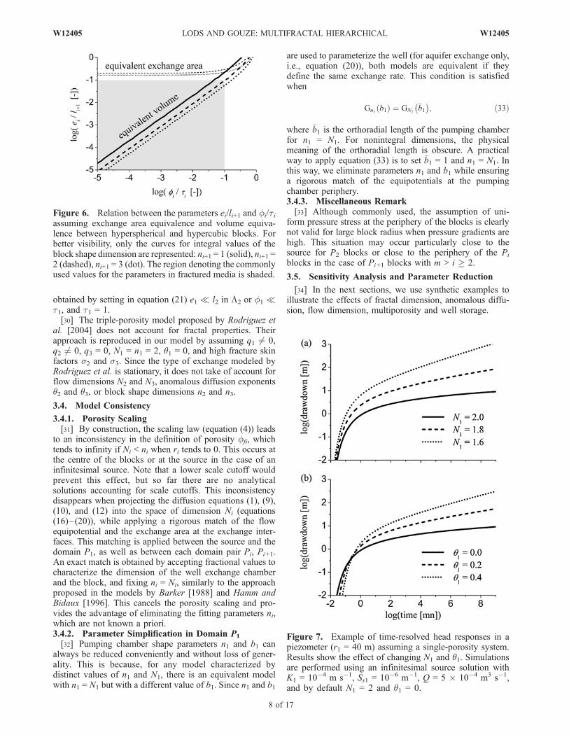
Figure 6. Relation between the parameters ei/li+1 and fi/tiassuming exchange area equivalence and volume equiva-lence between hyperspherical and hypercubic blocks. Forbetter visibility, only the curves for integral values of theblock shape dimension are represented: ni+1 = 1 (solid), ni+1 =2 (dashed), ni+1 = 3 (dot). The region denoting the commonlyused values for the parameters in fractured media is shaded.

Figure 7. Example of time-resolved head responses in apiezometer (r1 = 40 m) assuming a single-porosity system.Results show the effect of changing N1 and q1. Simulationsare performed using an infinitesimal source solution withK1 = 10�4 m s�1, Ss1 = 10�6 m�1, Q = 5 � 10�4 m3 s�1,and by default N1 = 2 and q1 = 0.

8 of 17


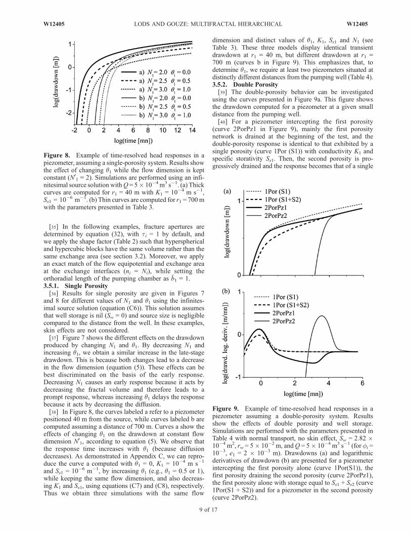
[35] In the following examples, fracture apertures aredetermined by equation (32), with ti = 1 by default, andwe apply the shape factor (Table 2) such that hypersphericaland hypercubic blocks have the same volume rather than thesame exchange area (see section 3.2). Moreover, we applyan exact match of the flow equipotential and exchange areaat the exchange interfaces (ni = Ni), while setting theorthoradial length of the pumping chamber as �b1 = 1.3.5.1. Single Porosity[36] Results for single porosity are given in Figures 7

and 8 for different values of N1 and q1 using the infinites-imal source solution (equation (C6)). This solution assumesthat well storage is nil (Sw = 0) and source size is negligiblecompared to the distance from the well. In these examples,skin effects are not considered.[37] Figure 7 shows the different effects on the drawdown

produced by changing N1 and q1. By decreasing N1 andincreasing q1, we obtain a similar increase in the late-stagedrawdown. This is because both changes lead to a decreasein the flow dimension (equation (5)). These effects can bebest discriminated on the basis of the early response.Decreasing N1 causes an early response because it acts bydecreasing the fractal volume and therefore leads to aprompt response, whereas increasing q1 delays the responsebecause it acts by decreasing the diffusion.[38] In Figure 8, the curves labeled a refer to a piezometer

positioned 40 m from the source, while curves labeled b arecomputed assuming a distance of 700 m. Curves a show theeffects of changing q1 on the drawdown at constant flowdimension N0

1, according to equation (5). We observe thatthe response time increases with q1 (because diffusiondecreases). As demonstrated in Appendix C, we can repro-duce the curve a computed with q1 = 0, K1 = 10�4 m s�1

and Ss1 = 10�6 m�1, by increasing q1 (e.g., q1 = 0.5 or 1),while keeping the same flow dimension, and also decreas-ing K1 and Ss1, using equations (C7) and (C8), respectively.Thus we obtain three simulations with the same flow

dimension and distinct values of q1, K1, Ss1 and N1 (seeTable 3). These three models display identical transientdrawdown at r1 = 40 m, but different drawdown at r1 =700 m (curves b in Figure 9). This emphasizes that, todetermine q1, we require at least two piezometers situated atdistinctly different distances from the pumping well (Table 4).3.5.2. Double Porosity[39] The double-porosity behavior can be investigated

using the curves presented in Figure 9a. This figure showsthe drawdown computed for a piezometer at a given smalldistance from the pumping well.[40] For a piezometer intercepting the first porosity

(curve 2PorPz1 in Figure 9), mainly the first porositynetwork is drained at the beginning of the test, and thedouble-porosity response is identical to that exhibited by asingle porosity (curve 1Por (S1)) with conductivity K1 andspecific storativity Ss1. Then, the second porosity is pro-gressively drained and the response becomes that of a single

Figure 8. Example of time-resolved head responses in apiezometer, assuming a single-porosity system. Results showthe effect of changing q1 while the flow dimension is keptconstant (N0

1 = 2). Simulations are performed using an infi-nitesimal source solution withQ = 5� 10�4 m3 s�1. (a) Thickcurves are computed for r1 = 40 m with K1 = 10�4 m s�1,Ss1 = 10�6 m�1. (b) Thin curves are computed for r1 = 700mwith the parameters presented in Table 3.

Figure 9. Example of time-resolved head responses in apiezometer assuming a double-porosity system. Resultsshow the effects of double porosity and well storage.Simulations are performed with the parameters presented inTable 4 with normal transport, no skin effect, Sw = 2.82 �10�4 m2, rw = 5� 10�2 m, andQ = 5� 10�4 m3 s�1 (for fi =10�3, e1 = 2 � 10�3 m). Drawdowns (a) and logarithmicderivatives of drawdown (b) are presented for a piezometerintercepting the first porosity alone (curve 1Por(S1)), thefirst porosity draining the second porosity (curve 2PorPz1),the first porosity alone with storage equal to Ss1 + Ss2 (curve1Por(S1 + S2)) and for a piezometer in the second porosity(curve 2PorPz2).


9 of 17

W12405

porosity model (curve 1Por(S1 + S2)) with conductivity K1

and specific storage Ss1 + Ss2. For a piezometer in thesecond porosity (curve 2PorPz2), the response is delayedand the late-time behavior is that of the model producingcurve 1Por(S1 + S2).[41] The logarithmic derivative of drawdown (@h/@ln(t))

is more sensitive than its primitive, thus providing anotherfitting curve that is helpful for discriminating the modeltype [Bourdet et al., 1983]. Figure 9b shows a plot of thelogarithmic derivatives. Wellbore storage produces an initiallinear increase, which, in the course of time, is followed bya decrease of the drawdown derivative. For a piezometerintercepting the first porosity, the double-porosity effect isexpressed as a U-shaped perturbation corresponding to theprogressive drainage of the second porosity. It can besuperimposed onto the wellbore storage effect.[42] Figure 10 presents curves illustrating the effects of

the parameters on the transition period without wellborestorage. This figure shows the drawdown logarithmicderivative for a piezometer intercepting the first porosityat a given small distance from the pumping well.[43] We observe that the U-shaped curves are related to

high values of Ss2 (Figures 10a, 10b, and 10e) and highvalues of t1 (Figure 10h). The end of the transition isdelayed when Ss2 increases because of the smaller blockdiffusivity. The time at which the transition starts decreaseswhen Ss2 increases. Indeed, higher values of Ss2 inducehigher exchanges caused by the smaller diffusivity in theblocks, which leads to higher head gradient at the interface.Similarly, higher values of t1 induce higher exchangescaused by the higher exchange area density. The effect ofchanging the exchange area density c2 can be parameterizedby t1 because t1 only appears in c2 (equation (21)). Highervalues of c2 (higher t1 in Figure 10h) brings forward thestart of the transition while not affecting the end of thetransition.[44] The V-shaped curves are related to high skin factors

(Figure 10i), and a high anomalous diffusion exponent(Figure 10f). The V shape is typical of the stationaryexchange model, which assumes instantaneous diffusionin the blocks. For high values of s2, the exchange iscontrolled by the reduction in permeability at the interface,rather than by the diffusive properties of the block. On theother hand, the diffusion increases with q2 because diffu-sivity increases from the block periphery to the centre. Notethe important advantage of using transient rather stationaryexchange model, since the latter allows V-shaped curvesonly.[45] A shift in time is produced by changing parameters

N2, s2, K2 and l2. The parameters N2 and s2 influence theamplitude of the transition perturbation, with higher N2

smoothing the transition (Figure 10c) and higher s2 pro-ducing a sharper transition (Figure 10i). K2 and l2 are the

only parameters that do not influence the amplitude of thetransition perturbation, since they produce a simple hori-zontal translocation (Figures 10d and 10g). Their effect onthe transition is the same. Indeed, in the first porositydrawdown (equation (24)), K2 and l2 only have an influenceon g1 (equation (28) with i = 1) via the terms l2g2l2

E2�1

and g2l2E2. In these terms, K2 and l2 can be combined

together intoffiffiffiffiffiffiK2

p/l21+q2/2, such that, for any value �K2 we

can find a value �l2 that keeps the first porosity drawdownunchanged:

�l2 ¼ l2 �K2=K2ð Þ1= 2þq2ð Þ ð34Þ

The curves (Figure 10g) are generated from Figure 10dusing equation (34). However, this procedure affects thedrawdown in the second porosity. Thus to carry out fittingwhen no data is available in the second porosity, one ofthese parameters can be assigned a fixed value. Otherwise,if data is available in the second porosity, the first porositydrawdown can be fitted first with one parameter fixed, andthen the second porosity drawdown can be fitted by relaxingthat parameter and adapting the other with equation (34).[46] The onset of the transition is affected by all the

parameters but q2 (Figure 10f). In detail, the onset of thetransition is delayed (1) by setting a smaller value of Ss2 ort1 as stated above, (2) by setting a smaller value of K2 or ahigher value of s2 which both decrease the exchange rate,and (3) by setting a smaller value of N2 or a higher value ofl2, which act as decreasing the exchange area density (21).[47] The end of the transition is affected by all the

parameters, except if K2 or Ss2 are modified while keepingx2 constant (Figure 10e) and by modifying t1 (Figure 10h).These two modifications produce the same effect, since theyboth ensure that the diffusivity equation (16, i = 2) remainsunchanged. Hence for any value of K2, it is possible to keepl2 constant by assigning:

t1 ¼ f1 þl2K1l

q2þ12

K2n2ð35Þ

The curves in Figure 10h are generated from Figure 10eusing equation (35). Thus for fitting, one of theseparameters can be fixed by assigning a value. However,the value of t1 is limited by two bounds and can lead tounrealistic fracture apertures. Since K2 is limited by onlyone bound, it is more convenient to fix t1 and vary K2. Notethat, because x2 and l2 are kept constant, the end of thetransition is unaffected by Ss2 when Ss1 + Ss2 remainsconstant for Ss1 � Ss2 (Figure 10b).[48] The above considerations lead to the following steps

to iterate for the inversion of parameters: (1) fit the end ofthe transition using K2, (2) fit the start of the transition usingSs2 with constant x2, (3) fit the shape of the transitionperturbation using N2, q2, and s2, and (4) fit the secondporosity drawdown using l2 and K2 (equation (34)).

Table 3. Parameters Used in Figure 8 Producing the Same

Transient Drawdown at r1 = 40 m

N1 (�) q1 (�) K1 (m/s) Ss1 (m�1)

2.0 0.0 10�4 10�6

2.5 0.5 5.446 � 10�5 1.345 � 10�7

3.0 1.0 3.333 � 10�5 1.875 � 10�8

Table 4. Parameters of Pi Domains Used for Figures 9 and 10

i Ki (m/s) Ssi (m�1) Ni (�) li (m) ri (m)

1 10�4 10�6 2 0.05 12 4 � 10�11 1.9 � 10�5 1 1 0

10 of 17


3.5.3. m Porosities (m > 2)[49] Figure 11a shows the responses of a piezometer in

the first domain of a triple-porosity system at a givendistance from a pumping well in a sedimentary aquifer. Inthese simulations, the well taps layer discontinuities (P1)delimiting planar blocks (P2), while these blocks are them-selves subdivided by vertical fractures that segregate porousmatrix sub-blocks (P3). The parameters given in Table 5represent standard values for karstic aquifer. In contrast tothe double-porosity effect (Figure 9), the response displayedby curve 3PorPz1(1) shows that the drainage of the thirdporosity can produce a second drawdown inflexion and asecond transition of the drawdown logarithmic derivative(Figure 11b). In a final stage, the behavior becomes iden-tical to that exhibited by a single porosity system (curve1Por(S1 + S2 + S3)), with conductivity K1 and specificstorage Ss1 + Ss2 + Ss3. The triple-porosity parameters haveeffects on the second transition period that are analogouswith those illustrated above for the transition period of thedouble-porosity model (Figure 10). The response displayedby curve 3PorPz1(2) shows that it can be difficult toinvestigate the triple-porosity effect using the drawdownlogarithmic derivative when there is a weak conductivitycontrast between domains.[50] More generally, for system with m domains,

the response of a piezometer in the first domain can show

m � 1 transitions of the drawdown logarithmic derivativebefore reaching a terminal behavior identical to thatobserved for a single porosity with conductivity K1 andspecific storage Ss1 + Ss2 + . . . + Ssm.

4. Conclusion and Remarks

[51] In the present model, we assume a nested distributionof fractured networks. Nested fracture models are a specificcase of multicontinuum models in which porosity domainsare hierarchically drained so the number of domain-to-domain flow exchange interfaces is equal to the numberof domain minus one. In the case of pumping tests, thehigher permeability domain will exchange flow with thepumping well. Each fractured network is characterized byits porosity and permeability, and may not only displayfractal geometry but also produce anomalous diffusion.Compared to others published models, the approach pre-sented here combines multifractal diffusion and multiporos-ity with transient exchanges, interface skin effects and wellstorage effects.[52] The proposed analytical solution in the Laplace

domain allows us to calculate drawdown at the pumpingwell and at any distance from the well for each porositylevel. After numerical inversion, the solution in the time-space domain yields a large spectrum of time-resolved

Figure 10. Example of time-resolved response of logarithmic derivatives of head in a piezometerintercepting the first porosity of a double-porosity system. Results show the effect of parameters on thetransition period, without well storage. Simulations are performed using the parameters presented inTable 4, with normal transport and no skin effect, rw = 5� 10�2 m andQ = 7.5� 10�4m3 s�1 (forf1 = 10

�3,e1 = 2 � 10�3 m). The curves are computed by modifying only the parameters specified in the legend:(a) Ss2, (b) Ss2 with constant SsTot = Ss1 + Ss2, (c) N2, (d) K2, (e) K2 and Ss2 with constant x2 = K2/Ss2,(f) q2, (g) l2, (h) t1, (i) s2.


11 of 17

W12405

drawdown curves, including those obtained using the mod-els by Barker [1988], Chang and Yortsos [1990], andHamm and Bidaux [1996]. While hydrology applicationsusually assume subdiffusion, with porosity, hydraulic con-ductivity, specific storativity and diffusivity decreasing as afunction of increasing radial distance, our model allows thestudy of superdiffusion in all the domains, with diffusivityincreasing as a function of increasing radial distance.[53] To ensure geometrical consistency and reduce the

number of fitting parameters, we introduce two conceptualapproaches:[54] 1. By applying the fractional dimension shape, we

generalize block and pumping well shapes to nonintegraldimensions, allowing an exact match between block periph-ery and within block equipotential, and also between the

pumping chamber periphery and external equipotentials. Atthe same time, we can eliminate the orthoradial length of thepumping chamber, which is an obscure parameter fornonintegral dimensions.[55] 2. Rules are defined for fracture-block complemen-

tation in order to ensure consistency between porosity,fracture aperture and block shape, while also eliminatingone of the fitting parameters (usually the fracture aperture).Equations are derived for both volume and exchange areaequivalence between hypercubic blocks and hypersphericalblocks. Yet we show that the volume equivalence modelis more pertinent to model fractured aquifers than theexchange area equivalence model. We point out that volumecomplementation was not addressed in previous modelingstudies. Provided volume complementation is performed,we can rigorously define the geometrical parameter tiaccounting for the occurrence of nonconductive zones(e.g., due to precipitation features or clogging).[56] While this model allows the simulation of a wide

range of situations, there are some remaining limitations.The main one is certainly the obligatory hierarchy of theproperties; conductivity of each fracture network must bedistinctly different from the others networks, but it is worthnoticing that fracture sets with weakly different conductiv-ities can be modeled by a single continuum with averagedproperties. Another limitation discussed in section 3.1 is theimpossibility to model linear drains because they do notsubdivide the embedding rock into segregated blocks, andthus they do not drain them peripherally. Also, as usual inthe analytical models (i.e., listed in Table 1) fractal scalecutoffs are not accounted for. In our model, the upper scalecutoff in the blocks is implicitly greater than the blockradius, but fractal properties are assumed to have no lowerscale cutoff.

Appendix A: Solutions in the Laplace Domain

[57] By applying a Laplace transform with respect to timeand using the initial conditions (equations (6) and (15)), weobtain from equations (16)–(19) the following diffusionequations:

p

xirqii~hi ¼

Ni � 1� qið Þri

d~hidri

þ d2~hidr2i

� liþ1rqii

d~hiþ1

driþ1

!riþ1¼1iþ1

; i < m; ðA1Þ

p

xmrqmm

~hm ¼ Nm � 1� qmð Þrm

d~hmdrm

þ d2~hmdr2m

; ðA2Þ

Table 5. Parameters of Pi Domains Used for Figure 11

i (1) Ki (m/s) (2) Ki (m/s) Ssi (m�1) Ni (�) li (m)

1 10�2 10�2 10�6 2 02 10�8 10�5 10�5 1 503 10�14 10�8 10�4 1 5

Figure 11. Example of time-resolved head responses in apiezometer (r1 = 200 m) intercepting the first porosity of atriple-porosity system. Results show the triple-porosityeffect. Simulations are performed with the parameterspresented in Table 5 with normal transport, no skin effect,no well effect, t1 = 1, rw = 5 � 10�2 m, and Q = 6.67 �10�3 m3 s�1. For a porosity value of 10�4, the fractureaperture values of the first and second porosities are 10�2

and 10�3 m, respectively. Drawdowns (a) and logarithmicderivatives of drawdown (b) are computed for a piezometerintercepting the first porosity alone (curve 1Por(S1)), thefirst porosity alone with storage equal to Ss1 + Ss2 (curve1Por(S1 + S2)), the first porosity alone with storage equal toSs1 + Ss2 + Ss3 (curve 1Por(S1 + S2 + S3)) and the firstporosity draining the second and third porosities, using theconductivities in Table 5(1) (curve 3PorPz1(1)), and theconductivities in Table 5(2) (curve 3PorPz1(2)).

12 of 17


the boundary conditions (7) and (8) are:

limr1!þ1

~h1 ¼ 0 ðA3Þ

limr1!0

rNi�ni�qii

@~hi@ri

!¼ 0; i > 1; ðA4Þ

the fracture skin equation (11) is:

~hi�1 ¼ ~hi þ lisid~hi=dri� �

ri¼li; i > 1; ðA5Þ

the pumping chamber mass balance differential equation (20)is:

Swp~hw ¼ Gn1 b1ð ÞrN1�1�q1w K1

d~h1dr1

!r1¼rw

þ Q

p; ðA6Þ

and the pumping chamber skin equation (13) is:

~hw ¼ ~h1 � rwswd~h1=dr1� �

r1¼rw: ðA7Þ

[58] For domain Pm, the general solution of equation (A2)is:

~hm ¼ C1mrnmEm

m Inm gmrEm

m

� �þ C2mr

nmEm

m Knm gmrEm

m

� �; ðA8Þ

where I and K are the modified Bessel functions of the firstand second kind, respectively, with C1i and C2i, i = 1, . . ., m,are integration variables, while assuming the following:

Em ¼ 2þ qmð Þ=2; ðA9Þ

nm ¼ 1� Nm= 2Emð Þ; ðA10Þ

gm ¼ffiffiffiffiffiffiffiffiffiffip=xm

p=Em: ðA11Þ

The auxiliary variables nm and gm must be finite. Thisimplies that Em must be nonzero and therefore qm 6¼ �2.Because qm should range in an interval containing 0, weassume qm > �2 in the following. For x, y, Z real, we use:

d=dZð Þ ZxIx yZð Þð Þ ¼ yZxIx�1 yZð Þ; ðA12Þ

d=dZð Þ ZxKx yZð Þð Þ ¼ �yZxKx�1 yZð Þ; ðA13Þ

yielding:

d~hm=drm ¼ gmEmrnmEmþEm�1m

�C1mInm�1 gmr

Em

m

� �� C2mKnm�1 gmr

Em

m

� ��:

ðA14Þ

Since nm � 1 < 0, and using the reflection formulae:

Kx Zð Þ ¼ K�x Zð Þ; Z > 0; ðA15Þ

Ix Zð Þ ¼ I�x Zð Þ þ 2 sin �xpð ÞK�x Zð Þ=p; Z � 0; ðA16Þ

we obtain, with sin(nmp) = sin((1 � nm)p):

d~hm=drm ¼ gmEmrnmEmþEm�1m C1mI1�nm gmr

Em

m

� ��þ 2C1m sin nmpð Þ=p� C2mð ÞK1�nm gmr

Em

m

� ��: ðA17Þ

Using the asymptotic behaviors:

Ix Zð Þ � Z=2ð Þx=G xþ 1ð Þ; x � 0; 0 � Z �ffiffiffiffiffiffiffiffiffiffiffixþ 1

p;

ðA18Þ

Kx Zð Þ � Z=2ð Þ�xG xð Þ=2; x > 0; 0 < Z �ffiffiffiffiffiffiffiffiffiffiffixþ 1

p;

ðA19Þ

we obtain for 0 < gmrmEm �

ffiffiffiffiffiffiffiffiffiffiffiffiffiffi2� nm

p:

d~hm=drm � h1C1mr2Em�1m þ h2 2C1m sin nmpð Þ=p� C2mð Þr2nmEm�1

m ;

ðA20Þ

where:

h1 ¼g2�nmm Em

21�nmG 2� nmð Þ ; ðA21Þ

h2 ¼gnmm EmG 1� nmð Þ

2nm: ðA22Þ

In equation (A20), h1 and h2 are not always zero becauseEm > 0, 1 � nm > 0, and gm > 0 for p > 0, so the boundarycondition (A4), (i = m) is satisfied for:

C2m ¼ 2C1m sin nmpð Þ=p; ðA23Þ

because Nm � nm � qm + 2nmEm � 1 is negative or nil, andfor:

Nm > nm � 1; ðA24Þ

such that Nm � nm � qm + 2Em � 1 > 0. Hence we obtain:

d~hm=drm ¼ C1mgmEmrnmEmþEm�1m I1�nm gmr

Em

m

� �; ðA25Þ

and with equation (A16):

~hm ¼ C1mrnmEm

m I�nm gmrEm

m

� �: ðA26Þ

The fracture skin equation (A5, i = m) with equation (A25)gives:

C1m ¼ ~hm�1=Am; ðA27Þ

where:

Am ¼ lnmEm

m I�nm gmlEm

m

� �þ lEm

m smgmEmI1�nm gmlEm

m

� �� ; ðA28Þ


13 of 17

W12405

which gives:

~hm ¼ ~hm�1rnmEm

m I�nm gmrEm

m

� �=Am: ðA29Þ

By substituting in the exchange term of domain Pm�1,combining equation (A25) with equation (A27) gives:

d~hm=drm� �

rm¼lm¼ ~hm�1Bm; ðA30Þ

where:

Bm ¼ �Am=Am; ðA31Þ

�Am ¼ lnmEmþEm�1m gmEmI1�nm gml

Em

m

� �: ðA32Þ

Using equation (A30), the diffusion equation (A1, i = m� 1)for domain Pm�1 can be written as:

p

xirqii~hi ¼

Ni � 1� qið Þri

d~hidri

þ d2~hidr2i

� liþ1rqii~hiBiþ1; i ¼ m� 1:

ðA33Þ

The general solution of equation (A33) is:

~hi ¼ C1irniEi

i Ini girEi

i

� �þ C2ir

niEi

i Kni girEi

i

� �; i ¼ m� 1;

ðA34Þ

where:

Ei ¼ 2þ qið Þ=2; i ¼ m� 1; ðA35Þ

ni ¼ 1� Ni=ð2EiÞ; i ¼ m� 1; ðA36Þ

gi ¼ffiffiffiffiffiffiffiffiffiffiffiffiffiffiffiffiffiffiffiffiffiffiffiffiffiffiffiffiffiffiffip=xi þ liþ1Biþ1

p=Ei; i ¼ m� 1: ðA37Þ

By applying the same reasoning as in domain Pm, we assumeqm � 1 > �2, so the boundary condition (A4, i = m � 1)implies:

C2i ¼ 2C1i sin nipð Þ=p; i ¼ m� 1; ðA38Þ

Ni > ni � 1; i ¼ m� 1: ðA39Þ

The fracture skin equation (A5, i = m � 1) gives:

C1i ¼ ~hi�1=Ai; i ¼ m� 1; ðA40Þ

where:

Ai ¼ lniEi

i I�ni gilEi

i

� �þ lEi

i sigiEiI1�ni gilEi

i

� �� ; i ¼ m� 1;

ðA41Þ

which gives:

~hi ¼ ~hi�1rniEi

i I�ni girEi

i

� �=Ai; i ¼ m� 1: ðA42Þ

For substituting in the exchange term of domain Pm � 2, weobtain:

d~hi=dri� �

ri¼li¼ ~hi�1Bi; i ¼ m� 1; ðA43Þ

where:

Bi ¼ �Ai=Ai; i ¼ m� 1; ðA44Þ

�Ai ¼ lniEiþEi�1i giEiI1�ni gil

Ei

i

� �; i ¼ m� 1: ðA45Þ

[59] Applying the same reasoning for domain Pi, 1 < i <m � 1 as for domain Pm�1, but with boundary conditions(A4, 1 < i < m � 1) and fracture skin equation (A5, 1 < i <m � 1), we obtain the following by recurrence, using i = m� 2, . . ., 2, for qi > �2 and Ni > ni �1:

~hi ¼ ~hi�1rniEi

i I�ni girEi

i

� �=Ai; i ¼ 2; . . .m� 2; ðA46Þ

d~hi=dri� �

ri¼li¼ ~hi�1Bi; i ¼ 2; . . . ;m� 2; ðA47Þ

where:

Ai ¼ lniEi

i I�ni gilEi

i

� �þ lEi

i sigiEiI1�ni gilEi

i

� �� ;

i ¼ 2; . . . ;m� 2;ðA48Þ

Bi ¼ �Ai=Ai; i ¼ 2; . . . ;m� 2; ðA49Þ

�Ai ¼ lniEiþEi�1i giEiI1�ni gil

Ei

i

� �; i ¼ 2; . . . ;m� 2; ðA50Þ

and:

Ei ¼ 2þ qið Þ=2; i ¼ 2; . . . ;m� 2; ðA51Þ

ni ¼ 1� Ni= 2Eið Þ; i ¼ 2; . . . ;m� 2; ðA52Þ

gi ¼ffiffiffiffiffiffiffiffiffiffiffiffiffiffiffiffiffiffiffiffiffiffiffiffiffiffiffiffiffiffiffip=xi þ liþ1Biþ1

p=Ei; i ¼ 2; . . . ;m� 2: ðA53Þ

[60] For domain P1, with equation (A47, i = 2), thediffusion equation (A1, i = 1) can be written as:

p

x1rq11

~h1 ¼N1 � 1� q1ð Þ

r1

d~h1dr1

þ d2~h1dr21

� l2rq11~h1B2: ðA54Þ

The general solution of equation (A54) is:

~h1 ¼ C11rn1E1

1 In1 g1rE1

1

� �þ C21r

n1E1

1 Kn1 g1rE1

1

� �: ðA55Þ

14 of 17


The boundary condition (A3) implies:

C11 ¼ 0: ðA56Þ

Using equation (A13), we obtain:

d~h1=dr1 ¼ �C21g1E1rn1E1þE1�11 Kn1�1 g1r

E1

1

� �: ðA57Þ

With equation (A57) and the pumping chamber skinequation (A7), we obtain:

C21 ¼ ~hw=A1; ðA58Þ

~h1 ¼ ~hwrn1E1

1 Kn1 g1rE1

1

� �=A1; ðA59Þ

where:

A1 ¼ ln1E1

1 Kn1 g1lE1

1

� �þ rwswg1E1l

E1�11 Kn1�1 g1l

E1

1

� �� : ðA60Þ

For substituting into the exchange term of the pumpingwell:

d~h1=dr1� �

r1¼rw¼ �~hwr

n1E1þE1�1w g1E1Kn1�1 g1r

E1

w

� �=A1: ðA61Þ

[61] Using equation (A61) and the pumping chambermass balance differential equation (A6), we obtain thedrawdown for the pumping well:

~hw ¼ QA1= p pSwA1 þ �A1ð Þ½ � ðA62Þ

where:

�A1 ¼ Gn1 b1ð ÞK1rN1=2w g1E1Kn1�1 g1r

E1

w

� �ðA63Þ

Appendix B: Consistency of Solutions

[62] In the drawdown solutions (equations (23), (24),(31)), all the quantities are positive except for ni, the skinfactors and possibly some modified Bessel functions of thefirst kind with negative order, which could lead to singu-larities for null denominators and negative square rootarguments. Nevertheless, drawdown solutions are alwayscalculable since all Bessel functions arguments are finite:

qi > �2¼)Ei > 0¼)gi > 0¼)0 � gilEi

i < þ1and 0 � gir

Ei

i < þ1

and the only term possibly including a modified Besselfunction of the second kind with null argument (blockcentre) is finite. Indeed, for ni > 0, and using the reflectionformula (A16), this term becomes:

rniEi

i I�ni girEi

i

� �¼ rniEi

i Ini girEi

i

� �þ 2 sin pnið Þ

�� Kni gir

Ei

i

� �=p�; ðB1Þ

then, for 0 � giriEi �

ffiffiffiffiffiffiffiffiffiffiffiffini þ 1

p, using the asymptotic

behaviors (equations (A18) and (A19)):

rniEi

i I�ni girEi

i

� �� gi=2ð Þni

G ni þ 1ð Þ r2niEi

i þ 2

psin pnið Þ

� G nið Þ2

gi2

� ��ni< þ1: ðB2Þ

Thus by recurrence, all drawdown solutions are finite.[63] In the numerical calculation of equations (23), (24),

and (31), Bessel function overflows can be avoided byapplying analytical reductions using reflection formulae(equations (A15) and (A16)) and asymptotic behaviors forlarge arguments:

Ix Zð Þ � exp Zð Þ=ffiffiffiffiffiffiffiffiffi2pZ

p; x � 0; x2 � 1=4

�� Z; ðB3Þ

Kx Zð Þ � exp �Zð Þ=ffiffiffiffiffiffiffiffiffiffiffip=2Z

p; x � 0; x2 � 1=4

�� Z:

ðB4Þ

Appendix C: Infinitesimal Source Solutionfor a Single Porosity

[64] For a single porosity, the infinitesimal source solu-tion is obtained from equation (24) by assuming a null wellstorage (Sw = 0) and taking the well exchange radius rw astending to 0. With equation (A15) and:

limZ!0

ZxKx Zð Þð Þ ¼ 2x�1G xð Þ; z > 0; ðC1Þ

D1 ¼ Qrn1E1

1 = Gn1 b1ð ÞK1E1�n11 D

n1=22 2�n1G 1� n1ð Þ

� �; ðC2Þ

D2 ¼ 1=x1 þ l2B2=p; ðC3Þ

we obtain for a single porosity (l2 = 0):

~h1 ¼ D1p�1�n1=2Kn1

ffiffiffiffiffiffiffiffipD2

prE1

1 =E1

� �: ðC4Þ

This can be inverted analytically using:

L1

2

Z

2

� �x

G �x;Z2

4t

� �� ¼ p�1�x=2Kx Z

ffiffiffip

p� �; ðC5Þ

where G(x, Z) is the complementary incomplete gammafunction, which gives:

h1 ¼ Qr2n1E1

1 G �n1; r2E1

1 =4E21x1t

� �= 4pn1=2b3�n1

1 K1E1G N1=2E1ð Þ=�

� G N1=2ð ÞÞ ðC6Þ

in which we usually assume n1 = N1 without loss ofgenerality, as stated in the discussion. Note that deriving theinfinitesimal source solution from a dimensionless finitesource solution is not possible because the dimensionlessradius r1/rw tends to infinity.


15 of 17

W12405

[65] At any given distance r1 from the well, two distinctmodels h1(N1, q1, K1, Ss1) and �h1(�N1, �q1, �K1, �Ss1) with thesame flow dimension (N0

1 = �N 01, n1 = �n1) have the same

transient drawdown h1(r1, t) = �h1(r1, t) for:

�K1 ¼ K1f �N 1; �q1� �

=f N1; q1ð Þ; ðC7Þ

�Ss1 ¼�K1

r2 �E1�E1ð Þ1 x1

�E1

E1

� �2

; ðC8Þ

where:

f N1; q1ð Þ ¼ r2n1E1

1 = pN1=2b3�N1E1G N1=2E1ð Þ=G N1=2ð Þ� �

: ðC9Þ

Notation

Subscriptsc CriticalC Cubicf Fractal scaling

i, j Porosity domain index‘ Laminarm Number of porosity domainss SpecificS Sphericalt Turbulentw Pumping well

Variables and functionsAi Truncated block exchange area, m2

bi Orthoradial length, mci Total compressibility, m s2 kg�1

Di Truncated block density, m�3

ei Fracture aperture of domains Pi<m, mG Unit-radius hyperspherical block or pumping

chamber area functionhi Drawdown in domains Pi=w,1,. . .,m, mH Heaviside functionIx Modified Bessel function of the first kind and

order xki Fractal permeability, m2 + qi

Kfi Hydraulic conductivity, m s�1

Ki Hydraulic conductivity on a unit-radius hyper-sphere, m1�Ni+ni+qi s�1

Kx Modified Bessel function of the second kind andorder x

l1 rw, mli Hyperspherical block radius of domains Pi>1, m�li Hypercubic block half-thickness of domains

Pi>1, mL Laplace transformm Number of porosity domains, �n1 Euclidean limit dimension of domain P1 and

pumping chamber shape dimension, �ni Block shape dimension of domains Pi>1, �Ni Fractal density dimension, �N0

i Flow or spectral dimension, �pw Pumping chamber nonlinear head loss exponent,

�p Laplace variable

Pi Porosity domain i, �Q Injection flow rate, negative for pumping, m3 s�1

Qc Critical flow rate, m3 s�1

qi Exchange flow rate density between Pi<m andPi+1, s

�1

r1 Radial Euclidean distance from the source center,m

ri Radial Euclidean distance from the symmetrycentre of blocks embedding Pi>1, m

rw Pumping well exchange radius, mSsfi Specific storage, m�1

Ssi Specific storage on a unit-radius hypersphere,m1�Ni+ni

Sw Pumping well capacity, m2

t Time elapsed from start of pump test, sVi Truncated block volume, m3

an 2pn/2/G(n/2)bi Correction factors for block radius li>1, �G Gamma function.Di Volume density of blocks Pi>1, �qi Anomalous diffusion exponent, �q0i Random walk dimension, �

li+1 Exchange coefficient between Pi < m andPi+1, m

Ni � ni � qi � 1

Li Exchange area density of blocks embeddingPi>1, m

�1

m Fluid dynamic viscosity, m�1 s�1 kgti Effective fracture volume ratio, �xi Diffusivity on a unit radius hypersphere,

m2+qi s�1

�r Fluid voluminal weight, kg m�2 s�2

s1 sw, �si Fracture skin factor between Pi > 1 and Pi � 1

sw Pumping chamber skin factor, �sw‘ Pumping chamber linear (laminar) skin factor, �swt Pumping chamber nonlinear (turbulent) skin

factor, m3(1�pw) spw�1

ffi Fracture fractal density or porosity, �fi Fracture fractal density or porosity on a unit

radius hypersphere, mni�Ni

ci Exchange area density between Pi >1 and Pi�1,m�1

[66] Acknowledgments. The authors wish to thank the reviewers,Rajagopal Raghavan, and anonymous for their helpful comments.

ReferencesAbdassah, D., and I. Ershaghi (1986), Triple-porosity systems for represent-ing naturally fractured reservoirs, SPE Form. Eval. Trans. AIME, 284,113–127.

Acuna, J. A., and Y. C. Yortsos (1995), Application of fractal geometry tothe study of networks of fractures and their pressure transient, WaterResour. Res., 31(3), 527–540.

Bai, M., D. Elsworth, and J.-C. Roegiers (1993), Multiporosity/multiperme-ability approach to the simulation of naturally fractured reservoirs, WaterResour. Res., 29(6), 1621–1633.

Barenblatt, G. R., I. P. Zheltov, and I. N. Kochina (1960), Basic concepts inthe theory of seapage of homogeneous liquids in fractured rocks, J. Appl.Math. Mech. Eng. Transl., 24(5), 1286–1303.

Barker, J. A. (1985a), Generalized well function evaluation for homoge-neous and fissured aquifers, J. Hydrol., 76, 143–154.

Barker, J. A. (1985b), Block-geometry functions characterizing transport indensely fissured media, J. Hydrol., 77, 263–279.

Barker, J. A. (1988), A generalized radial flow model for hydraulic tests infractured rock, Water Resour. Res., 24(10), 1796–1804.

Barton, C. C., and P. A. Hsieh (1989), Physical and Hydrological-FlowProperties of Fractures, Guidebook T385, AGU, Las Vegas, Nev.

16 of 17


Bernard, S., F. Delay, and G. Porel (2006), A new method of data inversionfor the identification of fractal characteristics and homogenization scalefrom hydraulic pumping tests in fractured aquifers, J. Hydrol., 328(3–4),647–658.

Boulton, N. S., and T. D. Streltsova (1977), Unsteady flow to a pumpedwell in a fissured water-bearing formation, J. Hydrol., 35, 257–269.

Bourdet, D., J. A. Ayoub, T. M. Whittle, Y. M. Pirard, and V. Kniazeff(1983), Interpreting well tests in fractured reservoirs, World Oil, 1975,77–87.

Camacho-Velazquez, R., M. Vasquez-Cruz, R. Castrejon-Aivar, andV. Arana-Ortiz (2005), Pressure-transient and decline-curve behaviorsin naturally fractured vuggy carbonate reservoirs, SPE Reservoir Eval.Eng., 8(2), 95–112.

Chang, J., and Y. C. Yortsos (1990), Pressure-transient analysis of fractalreservoirs, SPE Form. Eval., 5, 31–38.

Chelidze, T., and Y. Gueguen (1990), Evidence of fractal fracture, Int. J.Rock Mech. Miner. Sci. Geomech. Abstr., 27(3), 223–225.

Closmann, P. J. (1975), An aquifer model for fissured reservoirs, SPE J.,15(5), 385–398.

de Dreuzy, J.-R., and P. Davy (2007), Relation between fractional flowmodels and fractal or long-range 2-D permeability fields, Water Resour.Res., 43, WO4431, doi:10.1029/2006WR005236.

Delay, F., A. Kaczmaryk, and P. Ackerer (2007), Inversion of interferencehydraulic pumping tests in both homogeneous and fractal dual media,Adv. Water Resour., 30(3), 314–334.

Hamm, S.-Y., and P. Bidaux (1996), Dual-porosity fractal models for tran-sient flow analysis in fractured rocks, Water Resour. Res., 32(9), 2733–2745.

Havlin, S., and D. Ben-Avraham (1987), Diffusion in disordered media,Adv. Phys., 36, 695–798.

Le Borgne, T., O. Bour, J. R. de Dreuzy, P. Davy, and F. Touchard (2004),Equivalent mean flow models for fractured aquifers: Insights from apumping tests scaling interpretation, Water Resour. Res., 40(3),W03512, doi:10.1029/2003WR002436.

Liu, J. C., G. S. Bodvarsson, and Y. S. Wu (2003), Analysis of flowbehavior in fractured lithophysal reservoirs, J. Contam. Hydrol., 62–63, 189–211.

Lods, G., and P. Gouze (2004), WTFM, software for well test analysis infractured media combining fractional flow with double porosity andleakance, Comput. Geosci., 30, 937–947.

Mandelbrot, B. B. (1983), The Fractal Geometry of Nature, 468 pp., W.H.Freeman, New York.

Moench, A. F. (1984), Double porosity models for a fractured groundwaterreservoir with fracture skin, Water Resour. Res., 20(7), 831–846.

Nolte, D. D., L. J. Pyrak-Nolte, and N. G. M. Cook (1989), The fractalgeometry of flow paths in natural fractures in rock and the approach topercolation, Pure Appl. Geophys., 131, 111–138.

O’Shaughnessy, B., and I. Procaccia (1985), Diffusion on fractals, Phys.Rev. A, 32(4), 3073–3083.

Papadopulos, I. S., and H. H. Cooper Jr. (1967), Drawdown in a well oflarge diameter, Water Resour. Res., 3(1), 241–244.

Pulido, H., F. Samaniego, J. Rivera, F. Diaz, and G. Galicia (2006), Welltest analysis for naturally fractured reservoirs with transient interporositymatrix, microfractures, and fractures flow, in Proceedings of the Thirty-First Workshop on Geothermal Reservoir Engineering, Stanford Univ.,Calif., Jan. 30–Feb. 1, SGP-TR-179.

Pulido, H., F. Samaniego, H. Cinco-Ley, J. Rivera, F. Diaz, and G. Galicia(2007), Triple-porosity model-dual permeability with transient hydraulicdiffusivity in naturally frectured reservoirs, in Proceedings of theThirty-Second Workshop on Geothermal Reservoir Engineering, StanfordUniv., Calif., Jan. 22–24, SGP-TR-183.

Rodriguez, F., V. Arana-Ortiz, and H. Cinco-Ley (2004), Well test charac-terization of small and large scale secondary porosity in naturally frac-tured reservoirs, SPE 90287, Annual technical conference and exhibition,Houston Texas, USA, Sept. 26–29.

Rorabaugh, M. J. (1953), Graphical and theoretical analysis of step-draw-down test of artesian well, Proc. Am. Soc. Civil Eng., 79(362), 23pp.

Sahimi, M., M. C. Robertson, and C. G. Sammis (1993), Fractal distribu-tion of earthquake hypocenters and its relation to fault patterns andpercolation, Phys. Rev. Lett., 70(14), 2186–2189.

Stehfest, H. (1970), Numerical inversion of Laplace transforms, Commun.ACM, 13(1), 47–49.

Theis, C. V. (1935), The relation between the lowering of the piezometricsurface and the rate and duration of discharge of a well using groundwater storage, Trans. AGU, 16, 519–526.

Turcotte, D. L. (1986), Fractals and fragmentation, J. Geophys. Res,91(B2), 1921–1926.

van Everdingen, A. F. (1953), The skin effect and its influence on theproductive capacity of a well, Trans. AIME, 198, 171–176.

Walker, D., and R. Roberts (2003), Flow dimensions corresponding tohydrogeologic conditions, Water Resour. Res., 39(12), 1349,doi:10.1029/2002WR001511.

Warren, J. E., and P. J. Root (1963), The behaviour of naturally fracturedreservoirs, SPE J., 3(2), 245–255.

��P. Gouze and G. Lods, Laboratoire Geosciences, Universite Montpellier

2 - CNRS, Subsurface, Pl. Bataillon, 34095 Montpellier Cedex 5, France.([email protected]; [email protected])


17 of 17

W12405

A generalized solution for transient radial flow in hierarchical multifractal fractured aquifers

Documents