A General Study of the Complex Ginzburg-Landau Equation Weigang Liu Dissertation submitted to the Faculty of the Virginia Polytechnic Institute and State University in partial fulfillment of the requirements for the degree of Doctor of Philosophy in Physics Uwe C. T¨auber, Chair Shengfeng Cheng Vito W. Scarola Eric R. Sharpe May 3rd, 2019 Blacksburg, Virginia Keywords: complex Ginzburg-Landau equation, critical dynamics, initial-slip exponent, aging scaling, nucleation phenomena Copyright 2019, Weigang Liu

Welcome message from author
This document is posted to help you gain knowledge. Please leave a comment to let me know what you think about it! Share it to your friends and learn new things together.
Transcript
A General Study of the Complex Ginzburg-Landau Equation
Weigang Liu
Dissertation submitted to the Faculty of the
Virginia Polytechnic Institute and State University
in partial fulfillment of the requirements for the degree of
Doctor of Philosophy
in
Physics
Uwe C. Tauber, Chair
Shengfeng Cheng
Vito W. Scarola
Eric R. Sharpe
May 3rd, 2019
Blacksburg, Virginia
Keywords: complex Ginzburg-Landau equation, critical dynamics, initial-slip exponent,
aging scaling, nucleation phenomena
Copyright 2019, Weigang Liu
A General Study of the Complex Ginzburg-Landau Equation
Weigang Liu
(ABSTRACT)
In this dissertation, I study a nonlinear partial differential equation, the complex Ginzburg-
Landau (CGL) equation. I first employed the perturbative field-theoretic renormalization
group method to investigate the critical dynamics near the continuous non-equilibrium tran-
sition limit in this equation with additive noise. Due to the fact that time translation
invariance is broken following a critical quench from a random initial configuration, an inde-
pendent “initial-slip” exponent emerges to describe the crossover temporal window between
microscopic time scales and the asymptotic long-time regime. My analytic work shows that
to first order in a dimensional expansion with respect to the upper critical dimension, the
extracted initial-slip exponent in the complex Ginzburg-Landau equation is identical to that
of the equilibrium model A. Subsequently, I studied transient behavior in the CGL through
numerical calculations. I developed my own code to numerically solve this partial differential
equation on a two-dimensional square lattice with periodic boundary conditions, subject to
random initial configurations. Aging phenomena are demonstrated in systems with either
focusing and defocusing spiral waves, and the related aging exponents, as well as the auto-
correlation exponents, are numerically determined. I also investigated nucleation processes
when the system is transiting from a turbulent state to the “frozen” state. An extracted
finite dimensionless barrier in the deep-quenched case and the exponentially decaying dis-
tribution of the nucleation times in the near-transition limit are both suggestive that the
dynamical transition observed here is discontinuous. This research is supported by the U.
S. Department of Energy, Office of Basic Energy Sciences, Division of Materials Science and
Engineering under Award DE-FG02-SC0002308

A General Study of the Complex Ginzburg-Landau Equation
Weigang Liu
(GENERAL AUDIENCE ABSTRACT)
The complex Ginzburg-Landau equation is one of the most studied nonlinear partial dif-
ferential equation in the physics community. I study this equation using both analytical
and numerical methods. First, I employed the field theory approach to extract the critical
initial-slip exponent, which emerges due to the breaking of time translation symmetry and
describes the intermediate temporal window between microscopic time scales and the asymp-
totic long-time regime. I also numerically solved this equation on a two-dimensional square
lattice. I studied the scaling behavior in non-equilibrium relaxation processes in situations
where defects are interactive but not subject to strong fluctuations. I observed nucleation
processes when the system under goes a transition from a strongly fluctuating disordered
state to the relatively stable “frozen” state where its dynamics cease. I extracted a finite
dimensionless barrier for systems that are quenched deep into the frozen state regime. An
exponentially decaying long tail in the nucleation time distribution is found, which suggests
a discontinuous transition. This research is supported by the U. S. Department of Energy,
Office of Basic Energy Sciences, Division of Materials Science and Engineering under Award
DE-FG02-SC0002308

I dedicate this thesis to my beloved parents.
v
Acknowledgments
I am deeply grateful to my advisor, Prof. Uwe C. Tauber, for his tremendous help and
support which extend from my research to my life. I benefited a lot from his philosophic
feedback, sustained guidance during my Ph. D study, and especially his help in fixing my
language problems. He kept encouraging me to practice my research skill and develop a more
comprehensive understanding about physics. With his endorsement, I was also pursuing
another related master degree in computer science, which also contributes to my study in
physics the other way round. In a word, I am very proud of being in his group and working
with him.
I would like to further express my gratitude to my PhD committee members: Prof. Eric
Sharpe, Prof. Vito Scarola, and Prof. Shengfeng Cheng, for their kindly comments on my
work and help on my study. I also thank Prof. Sebastian Diehl, Prof. Andrea Gambassi, Prof.
Hannes Janssen, Prof. Michel Pleimling, and Dr. Lukas Sieberer for helpful discussions.
I want to thank people in our group, for their constructive suggestions. I thank our graduate
program coordinator, Betty Wilkins, and program support technician, Katrina Loan. My
thanks extend to our IT staff members including Roger Link and Travis Heath. I especially
wish to thank Dr. Hiba Assi, Dr. Priyanka and Dr. Jacob Carroll for their careful critical
reading of chapters in the dissertation.
I thank the the U. S. Department of Energy, since all those projects are supported by the
vi
U. S. Department of Energy, Office of Basic Energy Sciences, Division of Materials Science
and Engineering under Award DE-FG02-SC0002308
I would like to thank all my friends in my study and my life, practically to my roommates
Chengyuan Wen, Wei Zhao, Xiangwen Wang and Wenchao Yang.
I am specially grateful to Jie Qu.
Finally, I express my thankfulness to my parents for their endless love.
vii

Contents
List of Figures xi
List of Tables xvi
1 Introduction 1
1.1 Non-equilibrium physics . . . . . . . . . . . . . . . . . . . . . . . . . . . . . 1
1.2 The complex Ginzburg-Landau equation . . . . . . . . . . . . . . . . . . . . 3
1.3 Critical initial-slip and aging phenomena . . . . . . . . . . . . . . . . . . . . 7
1.4 Classical nucleation theory . . . . . . . . . . . . . . . . . . . . . . . . . . . . 8
1.5 Structure of this thesis . . . . . . . . . . . . . . . . . . . . . . . . . . . . . . 9
2 Critical initial-slip scaling for the noisy complex Ginzburg–Landau equa-
tion 10
2.1 Introduction . . . . . . . . . . . . . . . . . . . . . . . . . . . . . . . . . . . . 11
2.2 Model description and mean-field analysis . . . . . . . . . . . . . . . . . . . 16
2.3 Renormalization group analysis to one-loop order . . . . . . . . . . . . . . . 24
viii

2.4 Effect of two-loop and higher-order fluctuation corrections . . . . . . . . . . 28
2.5 Spherical model . . . . . . . . . . . . . . . . . . . . . . . . . . . . . . . . . . 30
2.6 Conclusion and outlook . . . . . . . . . . . . . . . . . . . . . . . . . . . . . . 33
3 Aging phenomena in the two-dimensional complex Ginzburg-Landau equa-
tion 35
3.1 Introduction . . . . . . . . . . . . . . . . . . . . . . . . . . . . . . . . . . . . 35
3.2 Model description . . . . . . . . . . . . . . . . . . . . . . . . . . . . . . . . . 38
3.3 Numerical scheme . . . . . . . . . . . . . . . . . . . . . . . . . . . . . . . . . 40
3.4 Results . . . . . . . . . . . . . . . . . . . . . . . . . . . . . . . . . . . . . . . 41
3.5 Conclusion . . . . . . . . . . . . . . . . . . . . . . . . . . . . . . . . . . . . . 47
4 Nucleation of spatio-temporal structures from defect turbulence in the
two-dimensional complex Ginzburg–Landau equation 49
4.1 Introduction . . . . . . . . . . . . . . . . . . . . . . . . . . . . . . . . . . . . 49
4.2 Model Description . . . . . . . . . . . . . . . . . . . . . . . . . . . . . . . . 53
4.3 Numerical Scheme and Nucleation Measurement . . . . . . . . . . . . . . . . 59
4.4 Spiral Structure Nucleation . . . . . . . . . . . . . . . . . . . . . . . . . . . 65
4.4.1 Quench Far Beyond the Defect Turbulence Instability Line . . . . . . 65
4.4.2 Quench Close To the Instability Line . . . . . . . . . . . . . . . . . . 73
4.5 Target Wave Nucleation . . . . . . . . . . . . . . . . . . . . . . . . . . . . . 76
ix
4.6 Conclusions . . . . . . . . . . . . . . . . . . . . . . . . . . . . . . . . . . . . 80
5 Conclusions 83
Bibliography 85
x

List of Figures
2.1 Full response propagator and one-particle reducible self-energy. . . . . . . . . 25
2.2 Feynman tadpole diagram or Hartree loop. . . . . . . . . . . . . . . . . . . . 27
2.3 Flow of the non-equilibrium parameter ∆(`) with initial values (a) ∆(1) =
0.01, (b) ∆(1) = 0.1, and (c) ∆(1) = 1.0 for several different initial values of
the non-linear coupling u(1) = 0.01, 0.1, 1.0, in d = 3 dimensions (ε = 1) and
rk(1) = 1.0. . . . . . . . . . . . . . . . . . . . . . . . . . . . . . . . . . . . . 29
2.4 Flow of the non-linear coupling parameter u(`) with initial values (a) u(1) =
0.01, (b) u(1) = 0.1, and (c) u(1) = 1.0 for several different initial values of
the non-equilibrium parameter ∆(1) = 0.01, 0.1, 1.0, in d = 3 dimensions
(ε = 1) and rk(1) = 1.0. . . . . . . . . . . . . . . . . . . . . . . . . . . . . . . 30
3.1 An example system configuration obtained from the solution of CGL on a two-
dimensional square lattice for the focusing spiral wave case when quenched
near the RGL limit with α = −0.05; β = 0.5 and t = 500. The white-red
plot (on the left) shows the amplitude of the complex order parameter; the
blue-white one depicts the phase. . . . . . . . . . . . . . . . . . . . . . . . . 41
xi

3.2 (a) The derivative of the logarithm of the characteristic length of the two-
dimensional CGL system with respect to the logarithm of the time, with
control parameters α = −0.05; β = 0.5, namely for focusing spirals. (b)
the scaled two-time autocorrelation function for various waiting time s. The
aging exponent here is b = 0.8. The blue dashed line with slope 1.49 is roughly
parallel to the collapsed curve, which indicates the autocorrelation exponent
λC/z = −1.49. The data result from averaging over 1000 independent runs. . 43
3.3 (a) The derivative of the logarithm of the characteristic length of the two-
dimensional CGL system with respect to the logarithm of the time, with
control parameters α = 1.176; β = 0.7, namely for defocusing spirals. (b)
the scaled two-time autocorrelation function for various waiting times s. The
aging exponent here is b = 0.25. These results were obtained by averaging
over 8000 independent runs. . . . . . . . . . . . . . . . . . . . . . . . . . . . 44
4.1 (a), (c): Number of topological defects n(t) and (b), (d) numerically deter-
mined characteristic length scale l(t), determined from the mean shock front
distances, as functions of numerical simulation time t, for systems with control
parameter pairs b = −3.5, c = 0.556 (a), (b); b = −3.5, c = 0.44 (c), (d). The
different graphs (with distinct colors) represent four independent realization
runs. The estimated nucleation threshold values for each plot were chosen ad
hoc “by hand and eye”: (a): nth = 385.0; (b): lth = 26.0; (c): nth = 735.0;
(d): lth = 27.0. . . . . . . . . . . . . . . . . . . . . . . . . . . . . . . . . . . 61
xii

4.2 Amplitude (red-white, left panel) and phase (white-blue, right panel) plots of
the complex order parameter A, for control parameters b = −3.5, c = 0.44.
The darkest points in the amplitude plot indicate the topological defects for
which |A| = 0, while the lightest color (almost white) here indicates the
shock line structures with steep amplitude gradients. The spiral structures
are clearly visible in the phase plot within the domains separated by the shock
fronts. . . . . . . . . . . . . . . . . . . . . . . . . . . . . . . . . . . . . . . . 62
4.3 (Left) Normalized distribution (histogram) P (Tn) of measured nucleation times
Tn for two-dimensional CGL systems with b = −3.5, c = 0.44 and different
sizes (varying from 256×256 to 640×640); here we set lth = 27 and ran 20, 000
realizations for each system size. (Middle) Extracted dimensionless nucleation
barrier ∆ as function of the inverse system size L−2 utilizing different values
for the tentative threshold lth; the dashed lines indicate a least-square fit for
the data points with the four largest system sizes. (Right) Infinite-size limit
(L → ∞) barrier ∆∞ vs. the prior selected threshold length lth; the (blue)
dashed line shows the least-square fit to Eq. (4.9) using the seven data points
with the smallest threshold lengths. . . . . . . . . . . . . . . . . . . . . . . . 66
4.4 From left to right: size-invariant dimensionless barrier ∆0, critical threshold
length lc, and exponent θ as functions of the control parameter b, with c =
−0.40 held fixed. These quantities are extracted by fitting our numerical data
to the empirical formula (4.10); the label “Direct quench” indicates that the
CGL systems here are directly quenched from random initial configurations
into the frozen regime. . . . . . . . . . . . . . . . . . . . . . . . . . . . . . . 69
xiii

4.5 From left to right: size-invariant dimensionless barrier ∆0, critical threshold
length lc, and exponent θ as functions of the control parameter c, with b =
−3.50 held fixed. The label “Quench from DT” (data plotted in red) indicates
that these systems were initialized in the defect turbulence regime with b =
−3.4 and c = 1.0, remained in this phase for a simulation time interval ∆t =
50, and were subsequently quenched into a frozen state characterized by the
parameter pairs (b, c) listed. . . . . . . . . . . . . . . . . . . . . . . . . . . . 70
4.6 Normalized nucleation time distributions P (Tn) for two-dimensional CGL sys-
tems with b = −3.5 and c = 0.556. Left panel: Data for varying the system
size L2 from 384×384 to 576×576, with ad-hoc selected nucleation threshold
length lth = 24. Right panel: Histograms for different nucleation thresholds
lth at fixed system size L = 384; 4, 000 independent realizations were run until
simulation time t = 2400 for each histogram. . . . . . . . . . . . . . . . . . . 73
4.7 Normalized nucleation time distribution P (Tn) for two-dimensional CGL sys-
tems with b = −3.5, c = 0.556, linear system size L = 384, and nucleation
threshold length lth = 24; 40, 000 independent realizations were run until
simulation time t = 2400. . . . . . . . . . . . . . . . . . . . . . . . . . . . . . 75
4.8 Amplitude (red-white, left panel) and phase (white-blue, right panel) plots
of the complex order parameter A, with bulk control parameters b = −1.4,
c = 0.9 in a 256 × 256 system; in the central 4 × 4 block, instead b = −1.4,
c = 0.6 (discernible as the small square structure with different coloring in the
center). The configuration is shown at numerical time t = 1200; in the left
panel, the lightest color (almost white) indicates shock line structures with
steep amplitude gradients. . . . . . . . . . . . . . . . . . . . . . . . . . . . . 77
xiv
4.9 (Left) Normalized nucleation time distribution P (Ts) for two-dimensional
CGL systems with bulk control parameter values set to b = −1.4 and c = 0.9,
whereas c = 0.6 in the central 4 × 4 patch, for varying linear system size
ranging from L = 384 to 576. Ts represents the measured nucleation time
adjusted by a size-dependent shift in order to achieve data collapse; we set
the nucleation threshold length to lth = 17.0, and ran 20, 000 independent
realizations for each system size. . . . . . . . . . . . . . . . . . . . . . . . . . 79
xv

List of Tables
3.1 Measured values of the dynamic, aging scaling, and autocorrelation exponents
for the focusing spiral case . . . . . . . . . . . . . . . . . . . . . . . . . . . . 43
3.2 Measured values of the dynamic, and aging scaling exponents for the defocus-
ing spiral case . . . . . . . . . . . . . . . . . . . . . . . . . . . . . . . . . . . 45
3.3 Measured values of the dynamic and aging scaling exponents for the defocusing
spiral case, near the limit α = β . . . . . . . . . . . . . . . . . . . . . . . . . 47
4.1 Number of systems that have nucleated successfully by computation time
t = 2, 400 among 20, 000 independent realizations for different system sizes. . 80
xvi

Chapter 1
Introduction
1.1 Non-equilibrium physics
A system in thermal equilibrium can be characterized in such a way that its stationary state
maximizes entropy (at fixed total energy), or minimizes free energy (at fixed temperature).
It evolves through the accessible configurations according to the its stationary probability
distribution. For example, in most realistic applications, systems are assumed to be coupled
to an external heat bath and thus are described by the canonical ensemble, for which the
stationary probability distribution P (E) is given by the Boltzmann factor
P (E) =1
Zexp(−E/kBT ), (1.1)
where E is the system energy, T is the temperature of the heat bath, Z is the partition
function, which provides a normalization factor for this probability distribution, and kB is
the Boltzmann constant. This ensemble can be used to describe the stationary distribution
of these systems; however, detailed information about the relaxation forwards equilibrium
1

not is not encoded. Therefore, there may exist multiple methods to successfully relax a
system toward the same stationary state governed by the Boltzmann distribution, even if the
accompanying dynamical properties can be quite different. A well-known example is that the
Ising model can be simulated on a computer using either Glauber or Metropolis dynamical
algorithms. Another important property of equilibrium models is that they always obey
detailed balance. Therefore, the probability currents between pair of accessible configurations
of the systems cancel each other so that there is direct reversibility between any two accessible
mircostates in this situation.
On the other hand, non-equilibrium dynamical systems are defined by the violation of de-
tailed balance in their microscopic processes [1]. The word “non-equilibrium” refers to situa-
tions for which there are non-vanishing net probability currents between different microstates.
But even those non-equilibrium systems can reach stationary states, where the Boltzmann
distribution may still hold and the concepts of equilibrium can still be applied. However,
there exist systems far from equilibrium for which detailed balance is violated so strongly
that the equilibrium physics approximation never becomes applicable. External particle
or energy currents drive systems out of equilibrium. Yet, these systems can reach macro-
scopic stationary states which need continuous particle or energy supply. Therefore, detailed
balance cannot be established in these non-equilibrium stationary states. Non-equilibrium
phase transitions, which are obtained through adjusting some control parameter(s) in such
non-equilibrium systems and separate distinct non-equilibrium stationary states, are not yet
fully classified. A quite general way to investigate the dynamics at a non-equilibrium tran-
sition is to initialize the system with a configuration that is far from equilibrium and let it
relax subsequently to its asymptotic stationary state [2], which is of the topic of our primary
interest in this dissertation.
Another important topic prominent in many non-equilibrium systems is pattern formation in
2
spatially extended settings. Roughly speaking, these are spatio-temporal features with char-
acteristic wave vector q0 and characteristic frequency ω0. The origin of pattern formation can
be intrinsic instabilities that arise when systems are brought away from their thermal equi-
librium by changing the associated control parameter(s) beyond their instability threshold,
or external noise. Theoretically, systems with control parameter(s) near the threshold can
be described by simple equations with a universal form, namely the “amplitude equation.”
However, in situation far beyond the threshold, it is sometimes possible to use simple “phase
equations” by perturbation of the original ideal periodic structures.
1.2 The complex Ginzburg-Landau equation
In this dissertation, we mainly focus on a stochastic non-linear partial differential equation,
the cubic complex Ginzburg-Landau equation (CGL),
∂A/∂t = (µr + iµi)A+ (αr + iαi)∇2A− (βr + iβi)|A|2A, (1.2)
where A is a complex order parameter that measures the amount of broken symmetry of
the system; µr indicates the deviation from the transition threshold; µi is a frequency shift;
αr and βr represent the diffusion constant and the nonlinear saturation, which are both
required to be positive; αi and βi measure the strength of linear and nonlinear dispersion
effects, respectively. Various phenomena can be described by this equation at least on a
qualitative level, such as second-order phase transitions, superfluidity, and superconductiv-
ity. It is also equivalent to the Gross-Pitaevskii equation with complex coefficients which
has been proposed to capture the open system-dynamics of driven-dissipative Bose-Einstein
condensation [3–5] if an additive complex noise term is also included in the equation, which
will be discussed in detail in Chapter 2.
3

There exist mainly two different approaches to study this non-linear equation, either ana-
lytically or numerically. A general framework for describing and understanding the complex
dynamics in this kind of systems using a field theory approach is discussed in Ref [6]. How-
ever, one can also try to solve this equation using numerical methods. We will present the
dynamic behavior of the CGL from numerical studies first. The analytic approach will be
covered in Chapter 2.
First of all, the symmetries that can be associated with this equation are time and space
translations, spatial reflections and rotations, and global gauge symmetry. Therefore, in a
certain phase away from the transition µr > 0, one can rescale the time and space variables,
as well as the complex field A according to these symmetries:
A′ =
√βrµrAeiµit,
t′ = µrt,
x′ =
√µrαr
x, (1.3)
and rewrite A′ → A, x′ → x, t′ → t, αi/αr → b and βi/βr → c. A reduced form of the
original CGL can be written in the form:
∂A/∂t = A+ (1 + ib)∇2A− (1 + ic)|A|2A, (1.4)
with only two real control parameters b and c left. This is the specific form that is usually
employed in numerical investigations. It is known as an amplitude equation that describes
“weekly nonlinear” spatiotemporal phenomena in the spatially extended case, especially
for dimension d = 1 or 2. Furthermore, Eq. (1.4) is invariant upon the transformation
(A, b, c) → (A∗,−b,−c). Therefore, only one half-plane in the (b, c) parameter space needs
to be considered. This equation can be also viewed as an extension of the “real” time-
4

dependent Ginzburg-Landau equation (RGL) [7]
∂A/∂t = A+∇2A− |A|2A (1.5)
by setting b = c = 0, as well as of the nonlinear Schrodinger equation (NLS)
i∂A/∂t = ∇2A± |A|2A (1.6)
in the limit b, c→∞.
The simplest solutions of Eq. (1.4) are plane waves [7]:
A =√
1−Q2 exp[i(Q · r − ωp(Q)t+ φ)],
F 2 = 1−Q2, ωp(Q) = c(1−Q2) + bQ2. (1.7)
Here φ is just a constant phase that can be chosen arbitrarily, due to the gauge symmetry.
Furthermore, for plane waves the amplitude F should be a real number, thus this solution
only exists for Q2 < 1.
These most standard solutions are rarely observed in numerical studies, because of the
spatiotemporal chaos that emerges prominently in CGL systems. Two different types of
chaotic fluctuation are encountered: One is called “phase chaos” where only the phase of the
complex order parameter A is dynamically active while the amplitude remains saturated.
This phase chaos is also known as phase turbulence and has, e.g., been studied by Manneville
and Chate [8]. On the other hand, phase chaos can transition into a “defect chaos” state
upon varying the control parameters (b, c) [9]. The term “defect” refers to topological defects,
which are characterized by zeros of the complex field A, enforcing singularities of the phase
θ = argA. Specifically in two dimensions, these singular topological defects are points with
5

integer topological charge m =∮L∇θdl/2π, where L is a contour around the zero point of
A, and m is used to quantify the singularity of the defect. Only single-charged defects with
m = ±1 are stable. Multi-charged defects will successively split into single-charged defects
[7]. The defect chaos, or “defect turbulence” state is then characterized by spontaneous
creation and annihilation of opposite-charged topological defects.
More common spatio-temporal structures in the CGL in two dimensions are spiral waves,
which are emitted by active topological defects. An isolated spiral solution was studied and
described by Hagan [10]:
A(r, θ, t) = F (r) exp[i(−ωt+mθ + ψ(r))], (1.8)
where (r, θ) are polar coordinates; m is the topological charge; ω is the rotation frequency
of the spiral, F (r) is the amplitude, and ψ(r) is the position-dependent phase of the spiral,
with the limiting forms:
F (r) → (1−Q2)12 , ψ′ → Q,ω = (1−Q2)c+ bQ2, as r →∞;
F (r) → arm, ψ′ → r, as r → 0. (1.9)
Hence the spiral wave solution will become plane-wave-like in the large-distance asymptotic
limit r →∞.
Another set of important structures that are also associated with spiral waves are “shocks.”
In two dimensions, they are nearly hyperbolic line structures [11] that separate different
spirals in space. As incoming fluctuations will be absorbed by these structures, there is no
information communication between different spirals. Those spiral structures, together with
shocks, eventually occupy the entire spatial domain, decimating all the defect turbulence.
Consequently,the dynamics becomes frozen, and this final state is called the “frozen” state
6
which is considered to persist indefinitely. However, there also exist active dynamical states
where spirals behave similarly to vortices in the dynamical XY model. In that regime, spirals
maintain an asymptotic wave length that is comparable to their typical extension; therefore,
no significant shocks can form in this situation.
Above, we have briefly introduced the states of the CGL that we are predominantly interested
in for this dissertation. We will further study these configurations in more detail in successive
chapters. We will also discuss related physical phenomena and properties that we intend to
investigate within the CGL framework.
1.3 Critical initial-slip and aging phenomena
The term “critical phenomena” is associated with the physics near a “critical point,” where
the characteristic correlation length diverges and relaxation processes slow down drastically.
They are often considered to take place near continuous (second-order) phase transitions [6].
Dynamical scaling, as well as universality, are described by critical exponents and scaling
functions. The “critical initial-slip” phenomenon emerges as the universal intermediate stage
of a relaxation process towards criticality from a disordered non-equilibrium initial state. It
is the crossover from the transient “initial-slip” to the asymptotic long-time regime that
can be characterized by the dynamic critical exponent z. It displays universal behavior and
can be (in some cases) described by a new independent critical exponent θ which emerges
due to the fact that time translation symmetry is broken by the initial configuration. It was
introduced and calculated by Janssen, Schaub, and Schmittmann [12] for an equilibrium non-
conserved order parameter system (namely, model A, according to Hohenberg and Halperin’s
classification [13], or RGL with additive noise).
Physical aging phenomena, as introduced by Struik’s [14] classical experimental study of the
7

slow dynamics of certain glass-forming systems, are observed in various systems with slow
relaxation dynamics [15]. They can be defined as follows: A physical system is considered to
undergo aging if the relaxation process satisfies three properties: slow dynamics, for example,
non-exponential decay; breaking of time-translation-invariance; dynamical scaling [16]. The
simple aging scaling form of the two time autocorrelation function C(t, s) = 〈φ(t)φ(s)〉 is
then given by:
C(t, s) = s−bfC(t/s), fC(y) ∼ y−λc/z, (1.10)
where φ is the order parameter and s � t is called waiting time, b is the aging exponent
while λC represents the autocorrelation exponent. The condition required for aging is very
similar to that of a critical initial-slip. In fact, the initial-slip exponent and autocorrelation
exponent can be connected by a scaling relation:
λC = d− θz (1.11)
in the equilibrium model A case.
1.4 Classical nucleation theory
Nucleation is considered to be the first step in a spontaneous first-order transition, beginning
with the metastability of the original initial state. It is generally suggested that there exists
a finite kinetic barrier for a discontinuous transition. Nucleation processes strongly rely on
rare events, the formation of “critical” nuclei, which describe the unstable state at the top of
the barrier. Classical nucleation theory (CNT) is a simple intuitive model that was proposed
around the middle of the 20th century [17, 18] and is described in detail in several reviews
[19–22]. It provides a quantitative description and explanation of related phenomena based
8

on appropriate approximations. The central result of CNT is a prediction of the nucleation
rate
R = ρZj exp
(−∆F
kBT
), (1.12)
where ∆F is the free energy cost of creating the critical nucleus, kB is Boltzmann’s constant
and T is the absolute temperature, ρ is the number density of nucleation sites, j is the rate
at which molecules attach to the nucleus, Z < 1.0 is the Zeldovich factor which describes
the probability that a nucleus at the top of the barrier will proceed to form the new state.
There are mainly two different kinds of nucleation: homogeneous nucleation which occurs in
the bulk of a pure phase, and heterogeneous nucleation that is triggered by impurities or on
surfaces. Homogeneous nucleation is much rarer than heterogeneous nucleation because the
nucleation barrier is much lower in the heterogeneous case.
1.5 Structure of this thesis
This dissertation is structured as follows. In Chapter 1, we provide a general introduction to
the model and phenomena that are studied in this thesis. An analytic study of the critical
initial-slip scaling in the CGL is presented in Chapter 2. We then numerically solve the
CGL on a two-dimensional square lattice. Using this approach, we investigate the associated
scaling and aging phenomena when shock structures are absent in the system in Chapter 3
and the nucleation processes when the system is transiting from the strong fluctuating defect
chaos state to a frozen state in Chapter 4. Finally, we provide an overall conclusion and
outlook for this general research topic in Chapter 5.
9

Chapter 2
Critical initial-slip scaling for the
noisy complex Ginzburg–Landau
equation
This chapter is based on our publication [23]:
Liu, Weigang and Tauber, Uwe C, “Critical initial-slip scaling for the noisy complex Ginzburg–
Landau equation,” Journal of Physics A: Mathematical and Theoretical 49, 434001 (2016).
Copyright (2016) by IOP Publishing.
I performed all the numerical work under Dr. Uwe C. Tauber’s supervision. All authors
contributed to the analytical calculations and writing of this paper.
10

2.1 Introduction
Physical systems display characteristic singularities when their thermodynamic parameters
approach a critical point. The ensuing singular behavior of various observables are gov-
erned by a considerable degree of universality: critical exponents and amplitude ratios are
broadly independent of the microscopic details of the respective systems. The emergence of
scale invariance, associated thermodynamic singularities, and universality near continuous
phase transitions is theoretically understood and described by the renormalization group
(RG), which also allows a systematic computation of critical exponents and associated scal-
ing functions (see, e.g., Refs. [24–27]). These concepts and theoretical tools can be extended
to dynamical critical behavior near equilibrium, which may similarly be grouped into var-
ious dynamical universality classes. In addition to global order parameter symmetries, the
absence or presence of conservation laws for the order parameter and its coupling to other
slow conserved modes crucially distinguish dynamical critical properties [6, 13, 28, 29]. More
recently, dynamical RG methods have been utilized to characterize various continuous phase
transitions far from thermal equilibrium as well [6, 30], including the associated universal
short-time or ‘initial-slip’ relaxation features and ‘aging’ scaling [16]. Yet a complete classi-
fication of non-equilibrium critical points remains an open task.
Our study is in part motivated by recent experimental realizations of systems with strong
light-matter coupling and a large number of degrees of freedom, which hold the potential
of developing into laboratories for non-equilibrium statistical mechanics, and specifically for
phase transitions among distinct non-equilibrium stationary states [31]. We mention a few
but significant examples: In ensembles of ultra-cold atoms, Bose–Einstein condensates placed
in optical cavities have allowed experimenters to achieve strong light-matter coupling and
led to the realization of open Dicke models [32, 33]. The corresponding phase transition has
been studied in real time, including the determination of an associated critical exponent [34].
11

Other platforms, which hold the promise of being developed into true many-body systems
by scaling up the number of presently available building blocks in the near future, are arrays
of microcavities [35–38] and also certain optomechanical setups [39–41]. Genuine many-
body ensembles in this latter class have been realized in pumped semiconductor quantum
wells placed inside optical cavities [42]. Here, non-equilibrium Bose–Einstein condensation of
exciton-polaritons has been achieved [43–45], where the effective bosonic degrees of freedom
result from the strong hybridization of cavity light and excitonic matter states [31, 46, 47].
Two essential ingredients are shared among these non-equilibrium systems [5]. First, they are
strongly driven by external fields and undergo a series of internal relaxation processes [31].
The irreversible non-equilibrium drive and accompanying balancing dissipation complement
the reversible Hamiltonian dynamics, and generate both coherent and dissipative dynamics
on an equal footing, albeit originating from physically quite independent mechanisms. The
additional irreversible terms cause manifest violations of the detailed-balance conditions
characteristic of many-body systems in thermal equilibrium, and induce the break-down of
the equilibrium Einstein relations that connect the relaxation coefficients with the thermal
noise strengths. Second, the particle number in these systems is not conserved due to
the coupling of the electromagnetic field to the matter constituents, thus opening strong
loss channels for the effective hybridized light-matter degrees of freedom. The resulting
quasi-particle losses must be compensated by continuous pumping in order to reach stable
non-equilibrium stationary states.
Interestingly, detailed-balance violations generically turn out to be irrelevant for purely re-
laxational critical dynamics of a non-conserved order parameter in the vicinity of continuous
phase transitions, which are hence characterized by the equilibrium model A universality
class [48]. Yet in systems that undergo driven-dissipative Bose-Einstein condensation, an
additional independent critical exponent associated with the non-equilibrium drive emerges,
12

which describes universal decoherence at large length- and time scales; it was originally iden-
tified by means of a functional RG approach [3, 4], and subsequently computed within the
perturbative RG framework [5]. This novel decoherence exponent should be observable in
the momentum- and frequency-resolved single-particle response that may, e.g., be probed in
homodyne detection of exciton-polaritons [49].
In d > 2 dimensions, the effective dynamical description or driven-dissipative Bose con-
densates utilizes a stochastic Gross–Pitaevskii equation with complex coefficients [3, 4], or,
equivalently, a complex time-dependent Ginzburg–Landau equation that generalizes the equi-
librium ‘model A’ relaxational kinetics [5]. The latter also features very prominently in the
mathematical description of spontaneous spatio-temporal pattern formation in driven non-
equilibrium systems [50, 51], and appears, for example, in the stochastic population dynamics
for three cyclically competing species (May–Leonard model without particle number conser-
vation) and related spatially extended evolutionary game theory systems [52]. Its critical
properties have previously been investigated in the context of coupled driven non-linear oscil-
lators that undergo a continuous synchronization transition at a Hopf bifurcation instability
[53]. Intriguingly, however, two-dimensional driven-dissipative Bose–Einstein condensation
appears to be captured by an anisotropic variant of the Kardar–Parisi–Zhang stochastic
partial differential equation [54].
An alternative and powerful method to extract dynamical critical exponents and identify
dynamical universality classes proceeds through the analysis of non-equilibrium relaxation
processes and the ensuing critical aging scaling [12, 16]. To this end, one prepares the
system initially in a fully disordered state with vanishing order parameter, and studies its
subsequent relaxation towards equilibrium or stationarity. The initial preparation breaks
time translation invariance; if the system is quenched near a critical point, the resulting
critical slowing-down renders relaxation times huge, whence the transient non-stationary
13

aging regime extends for very long time intervals, and this critical initial-slip regime is
governed by universal power laws [12, 55]. In the case of a non-conserved order parameter
or equilibrium model A in the terminology of Halperin and Hohenberg [13], this process
is in fact characterized by an independent critical initial-slip exponent θ and an associated
universal scaling function with a single non-universal scale factor [12]. We remark that the
original perturbative RG treatment for the critical universal short-time dynamics and aging
scaling has only just been extended towards a non-perturbative numerical analysis [56].
In contrast to model A relaxational kinetics, for dynamical critical systems with a conserved
order parameter, the aging scaling regime is entirely governed by the long-time asymptotic
stationary dynamical scaling exponents [12]; this is true also for models that incorporate
couplings to other slow conserved fields [57, 58]. Consequently, the initial-slip or aging
scaling regime provides a convenient means to quantitatively characterize critical dynamics
in numerical simulations (and presumably real experiments as well) during the system’s non-
equilibrium relaxation phase [59]. Non-equilibrium critical relaxation and aging scaling has
also been explored in driven systems that either display generic scale invariance, or are tuned
at a continuous phase transition point. Prominent examples include the Kardar–Parisi–
Zhang equation for driven interfaces or growing surfaces [60–62], driven diffusive systems
[61, 63], and reaction-diffusion or population dynamics models that display a transition to
an absorbing state, e.g., in the contact process [64], and stochastic spatially extended Lotka–
Volterra models for predator-prey competition, for which the emergence of aging scaling may
serve as an early-time indicator for the predator species extinction [65].
Inspired by these significant findings, in this present work we address the question if the uni-
versal non-equilibrium relaxation processes in the critical complex time-dependent Ginzburg–
Landau equation differ from the corresponding equilibrium dynamical model A ? In order to
attack this problem mathematically, we utilize the path integral representation of stochastic
14

Langevin equations through a Janssen–De Dominicis functional [6, 66–68], as previously de-
veloped and analyzed in the critical stationary regime for driven-dissipative Bose–Einstein
condensation in Ref. [5]. Following Ref. [12] for the initial-slip and aging scaling analysis
of the relaxational models A and B in thermal equilibrium, we represent the randomized
initial state through a Gaussian distribution for the complex-valued order parameter field.
We then employ the perturbative field-theoretical RG approach [24–27], and specifically its
extension to critical dynamics [6, 28, 29], to analyze the ensuing singularities and compute
the critical exponents. Since the initial conditions at time t = 0 may be viewed as specifying
sharp boundary conditions on the semi-infinite time sheet, one can borrow theoretical tools
originally developed for the investigation for surface critical phenomena [69]. Near and below
the upper critical dimension dc = 4, the parameter ε = 4 − d serves as the effective small
expansion parameter for the ensuing perturbation series in terms of non-linear fluctuation
loops.
The bulk part of this paper is organized as follows: In the following section 2.2, we provide
the mesoscopic dynamical model based on a stochastic Gross–Pitaevskii partial differential
equation with complex coefficients that is motivated by experimental studies on driven-
dissipative Bose–Einstein condensation [3, 4]. Equivalently, this non-equilibrium kinetics
can be viewed as relaxational model A dynamics of a non-conserved complex order parame-
ter field orginating from a complex-valued Landau–Ginzburg functional [5]. Then, utilizing
the harmonic Feynman diagram components, i.e., correlation and response propagators that
are constructed from the linear part of the associated Janssen–De Dominicis response func-
tional [12], we first discuss the system’s dynamics on the mean-field level, including the
fluctuation-dissipation ratio [55]. Section 2.3 details our perturbative RG calculation to low-
est non-trivial (one-loop) order in ε. Upon utilizing a additional renormalization constant
for the order parameter field on the ‘initial-time sheet,’ we obtain the scaling behavior of
15

our model and determine the additional independent initial-slip critical exponent associated
with a fully randomized initial state [12]. Through the extra renormalization constant ac-
quired by the initial preparation that induces breaking of time translation invariance, we
extract the initial-slip exponent which governs the universal short-time behavior as well as
the non-equilibrium relaxation in the aging scaling regime. We then proceed to discuss the
resulting two-loop and higher-order corrections through numerical solutions of the one-loop
RG flow equations for the non-linear coupling parameters [5] in section 2.4. In section 2.5,
we construct a suitable complex spherical model A extension akin to Ref. [70] to provide an
alternative demonstration for our main conclusion, namely that the critical aging scaling in
the non-equilibrium complex Ginzburg–Landau equation is asymptotically governed by the
equilibrium model A initial-slip exponent. We finally summarize our work in the concluding
section 2.6. A brief appendix lists the fundamental momentum loop integrals evaluated by
means of the dimensional regularization technique that are required for the perturbative
renormalization group calculations.
2.2 Model description and mean-field analysis
Following Refs. [3–5], we employ a noisy Gross–Pitaevskii equation with complex coefficients
to capture the dynamics of a Bose–Einstein condensate subject to dissipative losses and
compensating external drive:
i∂tψ(x, t) =[−(A− iD)∇2 − µ+ iχ+ (λ− iκ)|ψ(x, t)|2
]ψ(x, t) + ζ(x, t) . (2.1)
Obviously, eq. (2.1) coincides with the time-dependent complex Ginzburg–Landau equation,
which has been prominently employed to describe pattern formation in non-equilibrium
systems in the noise-free deterministic limit [50, 51]. The complex bosonic field ψ here
16

represents the polariton degrees of freedom. The complex coefficients have clear physical
meanings as well: χ = (γp − γl)/2 is the net gain, the balance of the incoherent pump rate
γp and the local single-particle loss rate γl. The positive parameters λ and κ represent the
two-body loss and interaction strength, respectively; and A = 1/2meff relates to the quasi-
particle effective mass. This stochastic partial differential equation is often not presented
with an explicit diffusion coefficient D, whereas a frequency-dependent pump term ∼ η∂tψ
is added on its left-hand side [71, 72], whereupon eq. (2.1) is recovered through dividing by
1− iη on both sides, i.e., with D = Aη and a subleading correction to the other coefficients,
which are complex to begin with. Due to the freedom of normalizing the time derivative term
as above in the equation of motion, this model accurately captures the physics close to the
phase transition, since it describes the most general low-frequency dynamics in a systematic
derivative expansion that incorporates all relevant coupling in dimensions d > 2 [5]. The
complex Gaussian white noise term ζ can be entirely characterized through its correlators
〈ζ∗(x, t)〉 = 〈ζ(x, t)〉 = 0 ,
〈ζ∗(x, t)ζ(x′, t′)〉 = γδ(x− x′)δ(t− t′) ,
〈ζ∗(x, t)ζ∗(x′, t′)〉 = 〈ζ(x, t)ζ(x′, t′)〉 = 0 . (2.2)
As mentioned above, the parameters A, D, λ, and κ should all be positive for physical
stability. On the other hand, the coefficient χ starts out negative initially and becomes
positive as the system undergoes a continuous driven Bose–Einstein condensation transition,
which results in a non-vanishing expectation value 〈ψ(x, t)〉 6= 0. The parameter µ, which
can be considered as an effective chemical potential, needs to stay fixed as a requirement for
stationarity. The Langevin equation (2.1) may be obtained from a microscopic description
in terms of a quantum master equation upon employing canonical power counting in the
17

vicinity of the critical point [3, 4, 73]. For analytical convenience, we introduce the following
ratios to rewrite the Gross–Pitaevskii equation:
r = − χD, r′ = − µ
D, u′ =
6κ
D, rK =
A
D, rU =
λ
κ. (2.3)
Factoring out iD on the right-hand side of (2.1), and iκ in front of the non-linear term, we
arrive at the equivalent stochastic partial differential equation
∂tψ(x, t) = −D[r + ir′ − (1 + irK)∇2 +
u′
6(1 + irU)|ψ(x, t)|2
]ψ(x, t)
+ξ(x, t) = −D δH[ψ]
δψ∗(x, t)+ ξ(x, t) . (2.4)
The stochastic noise term ξ = −iζ can be characterized similarly as ζ above. In the second
line, we have written eq. (2.4) in the form of purely relaxational kinetics with a non-
Hermitean effective ‘pseudo-Hamiltonian’
H[ψ] =
∫ddx
[(r + ir′)|ψ(x, t)|2 + (1 + irK)|∇ψ(x, t)|2
+u′
12(1 + irU)|ψ(x, t)|4
]. (2.5)
With the above assumptions, we can construct the equivalent dynamical Janssen–De Do-
minicis response functional [66–68] of this driven-dissipative model by introducing a Martin–
Siggia–Rose response field ψ(x, t) to average the stochastic noise ξ through a Gaussian in-
18
tegral; see, e.g., Ref. [6] for more detailed explanations:
A[ψ, ψ] =
∫ddx
∫dt
{ψ∗(x, t)
[∂t +D
(r + ir′ − (1 + irK)∇2
)]ψ(x, t)
+ψ(x, t)[∂t +D
(r − ir′ − (1− irK)∇2
)]ψ∗(x, t)
−γ2|ψ(x, t)|2 +D
u′
6(1 + irU)ψ∗(x, t)|ψ(x, t)|2 ψ(x, t)
+Du′
6(1− irU)ψ(x, t)|ψ(x, t)|2 ψ∗(x, t)
}. (2.6)
In addition to this bulk action [5], we must specify randomized initial configurations at the
t = 0 time sheet from which the system relaxes. To this end, we assume a Gaussian weight
for the initial order parameter field characterized by 〈ψ(x, 0)〉 = a(x) at the initial time
surface. In addition to taking averages with the bulk weight exp(−A[ψ, ψ]), we then require
averaging with the Gaussian probability distribution
e−Hi[ψ] = exp
[−∆
∫ddx |ψ(x, 0)− a(x)|2
], (2.7)
which specifies an initial state with mean spatially varying order parameter a(x) and the
correlations ⟨[ψ(x, 0)− a(x)
][ψ∗(x′, 0)− a∗(x′)
]⟩= ∆−1δ(x− x′) . (2.8)
We now set ψ(x, t < 0) = 0, whereupon the Gaussian part of the action (2.6) becomes
A0[ψ, ψ] =
∫ddx
∫ ∞0
dt
{ψ∗(x, t)
[∂t +D
(r + ir′ − (1 + irK)∇2
)]ψ(x, t)
+ψ(x, t)[∂t +D
(r − ir′ − (1− irK)∇2
)]ψ∗(x, t)− γ
2|ψ(x, t)|2
}. (2.9)
We finally complement the action with external source terms J and J conjugate to both the
19

ψ and ψ fields:
AJ [ψ, ψ] = −∫ddx
∫dt[J∗(x, t)ψ(x, t) + J∗(x, t)ψ(x, t)
+J(x, t)ψ∗(x, t) + J(x, t)ψ∗(x, t)]. (2.10)
Hence, the ultimate generating functional of our model becomes
Z[J , J ] =
∫D[iψ]
∫D[ψ] exp
[− (A[ψ, ψ] +Hi[ψ] + AJ [ψ, ψ])
]. (2.11)
We first analyze the mean-field theory for our model. By means of the Green’s function
technique, we may directly solve the classical field equations for the Gaussian generating
functional Z0[J , J ] to obtain the mean-field expressions for the expectation values 〈ψ(x, t)〉0and 〈ψ(x, t)〉0:
0 =δ(A0 +Hi + AJ)
δψ∗(x, t)=
[∂t +D
(r + ir′ − (1 + irK)
)∇2]ψ(x, t)
−J(x, t)− γ
2ψ(x, t) ,
0 =δ(A0 +Hi + AJ)
δψ∗(x, t)=
[−∂t +D
(r − ir′ − (1− irK)
)∇2]ψ(x, t)
−J(x, t)− ψ(x, 0)δ(t) + ∆[ψ(x, 0)− a(x)]δ(t) . (2.12)
The integration limit for the differential equations above is constrained to 0 < t < ∞, and
the boundary conditions for the Martin–Siggia–Rose response field ψ(x, t = 0) = ∆[ψ(x, 0)−
a(x)] and ψ(x, t→∞) = 0 are necessary to satisfy the initial distribution of ψ(x, 0). Solving
these time differential equations in momentum space, we find for 〈ψ(q, t)〉0 and 〈ψ(q, t)〉0 in
20

terms of the conjugate sources:
〈ψ(q, t)〉0 =
∫ ∞0
exp{D[r − ir′ + (1− irK)q2
](t− t′)
}Θ(t− t′)J(q, t′) dt′ ,
〈ψ(q, t)〉0 =
∫ ∞0
exp{−D
[r + ir′ + (1 + irK)q2
](t− t′)
}Θ(t− t′)
×[J(q, t) +
γ
2ψ(x, t) +
[a(q) + ∆−1ψ(q, t)
]δ(t)
]dt′ . (2.13)
Thus we determine the Gaussian response and correlation propagatorsG0ψ∗ψ
(q, t, t′) = 〈ψ∗(q, t)
ψ(q, t′)〉 = δ〈ψ(q, t′)〉/δJ(q, t)|J=J=0 and C0ψ∗ψ(q, t, t′) = 〈ψ∗(q, t′)ψ(q, t)〉 = δ〈ψ(q, t)〉/
δJ(q, t′) |J=J=0, which serve as the basic components for the perturbation expansion and
Feynman diagrams. By means of the expressions (2.13), we arrive at
G0ψ∗ψ
(q, t, t′) = G0ψ∗ψ
(q, t− t′) = e−D[r+ir′+(1+irK)q2](t−t′) Θ(t− t′) , (2.14)
C0ψ∗ψ(q, t, t′) = CD
ψ∗ψ(q, t, t′) + ∆−1G0ψ∗ψ
(q, t)G0ψψ∗
(q, t′) . (2.15)
Comparing with the bulk propagators of Ref. [5], the harmonic response propagator (2.14)
here is not influenced by the initial condition and remains translationally invariant in time,
whereas the correlation propagator (2.15), more precisely, its Dirichlet component CDψ∗ψ(q, t, t′),
distinctly reflects the initial preparation and does not obey time translation invariance,
CDψ∗ψ(q, t, t′) =
γ e−iD(r′+rKq2)(t−t′)
4D(r + q2)
[e−D(r+q2)|t−t′| − e−D(r+q2)(t+t′)
]. (2.16)
Under RG scale transformations, the initial configuration distribution width ∆ is a relevant
parameter, and one expects ∆ → ∞ under the renormalization group flow [12]. If this
asymptotic limit ∆→∞ is taken, the second term in C0ψ∗ψ(q, t, t′) becomes eliminated, and
we are left with only the Dirichlet correlator (2.16).
It is instructive to follow Ref. [55], and use the Gaussian response and correlation propagators
21
to evaluate the fluctuation-dissipation ratio
X(q; t > t′, t′) = kBTχ(q; t > t′, t′)
dC0ψ∗ψ(q; t, t′)/dt′
. (2.17)
In thermal equilibrium, this ratio is required to be 1 according to Einstein’s relation. To this
end, we require the dynamic susceptibility or response function
χ(q; t > t′, t′) = D(1 + irK)G0ψ∗ψ
(q, t, t′) , (2.18)
wherefrom we obtain the inverse fluctuation-dissipation ratio (2.17) in momentum space for
our model
X(q; t > t′, t′)−1 =γ
4DkBT (r + q2)(1 + irK)
[r + ir′ + (1 + irK)q2
+(r − ir′ + q2 − irKq2) e−2D(r+q2)t′]− r − ir′ + (1− irK)q2
∆(1 + irK)e−2D(r+q2)t′ . (2.19)
In the asymptotic time limit t′ →∞, this expression reduces to
limt′→∞
X(q; t > t′, t′)−1 =γ[r + ir′ + (1 + irK)q2]
4DkBT (r + q2)(1 + irK). (2.20)
In order to satisfy the fluctuation-dissipation theorem as required for the system to relax
towards thermal equilibrium at long times, one must thus demand the following relation-
ships between the parameters in the modified Gross–Pitaevskii or complex time-dependent
Ginzburg–Landau equation (2.4):
r′ = rKr , γ = 4DkBT . (2.21)
In the critical regime r = r′ = 0 and q2 = 0, where the characteristic relaxation time
22
scale tc = [D(r+ q2)]−1 diverges, the fluctuation-dissipation ratio (2.19) will never reach the
thermal equilibrium limit 1; in fact even with equilibrium parameters (2.21) it attains a fixed
complex value at any time t′,
X(0; t > t′, t′) =1 + irK
2. (2.22)
In the asymptotic Dirichlet limit ∆ → ∞, the fluctuation-dissipation ratio becomes in real
space
X0(x; t > t′, t′)−1 = 1 +1− irK1 + irK
(t− t′
t+ 1−irK1+irK
t′
)d/2
× exp
(−2Dt′
[r − x2
4D2(t− t′)(1 + irK)2(t+ 1−irK
1+irKt′)]) . (2.23)
This result yields the corresponding equilibrium model A expression for rK = 0 [55]. In the
long-time limit t, t′ → ∞, with the time ratio s = t′/t held fixed, we find near the critical
point r = 0,
X0(0; s = t′/t < 1)−1 = 1 +1− irK1 + irK
(1− s
1 + 1−irK1+irK
s
)d/2
. (2.24)
Thermal equilibrium is restored as s → 1. However, for s = 0 the ratio (2.22) is reached:
X0(0; 0)−1 = 1 + (1 − irK)/(1 + irK). This suggests a crossover between the time ratio
regimes s = 1 and s = 0, which can be associated with the critical initial slip exponent θ. In
the following section, we shall write down the associated general scaling laws, and explicitly
calculate θ for our specific model by means of the perturbative dynamical RG to one-loop
order, or first order in the dimensional expansion in ε = 4− d.
23

2.3 Renormalization group analysis to one-loop order
As established by Janssen, Schaub, and Schmittmann, the general scaling form in the initial-
slip or critical aging regime t′ � t for the dynamical correlation function of the equilibrium
model A for a non-conserved order parameter with purely relaxational kinetics reads
C(q; t, t′/t→ 0) = |q|−2+η (t/t′)θ−1 C0(qξ, |q|zDt) , (2.25)
where ξ ∼ |τ |−ν denotes the diverging correlation length as the critical point at τ = 0 is
approached, with associated critical exponent ν; z indicates the dynamical critical exponent
that describes critical slowing-down, while θ denotes the universal initial-slip exponent θ [12].
In thermal equilibrium, the fluctuation-dissipation theorem then yields the corresponding
scaling form for the dynamic susceptibility:
χ(q; t, t′/t→ 0) = D|q|z−2+η (t/t′)θ χ0(qξ, |q|zDt) Θ(t) . (2.26)
For the driven-dissipative Gross–Pitaevskii equation or complex Ginzburg–Landau equation,
the following more general scaling form applies for the dynamical response function [5]:
χ(q; t, t′/t→ 0) = D|q|z−2+η (1 + ia|q|η−ηc)−1 (t/t′)θ
×χ0
(qξ, |q|z(1 + ia|q|η−ηc)Dt
)Θ(t) . (2.27)
Here, the universal correction-to-scaling exponent ηc is induced by the external drive, and
describes the ultimate disappearance of coherent quantum fluctuations at the critical point
relative to the dissipative internal noise. To second order in the dimensional expansion, one
obtains ηc = −[4 ln(4/3) − 1 + O(ε)]η. Similar additional terms apply to the dynamical
correlation function (2.25), albeit in general with also modified Fisher exponent η → η′ and
24
q, 0 q, t ∑'
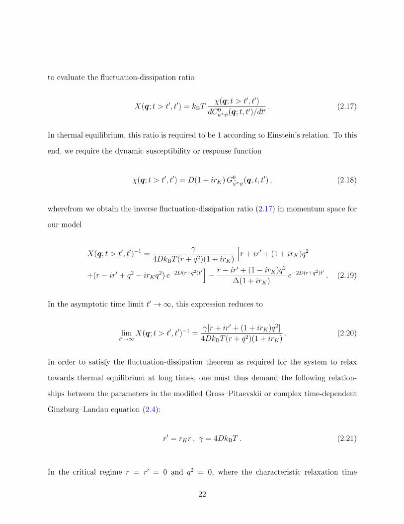
Figure 2.1: Full response propagator and one-particle reducible self-energy.
initial-slip exponent θ → θ′:
C(q; t, t′/t→ 0) = |q|−2+η′ (t/t′)θ′−1 C0(qξ, |q|zDt, a|q|η−ηc) . (2.28)
Yet both the perturbative and non-perturbative RG analysis have established that this sys-
tem eventually thermalizes in the critical regime, whereupon detailed balance becomes ef-
fectively restored. This thermalization, which requires that ∆ = rU − rK → 0, implies
the identities η′ = η and also θ′ = θ. In addition, asymptotically in fact rU = rK → 0
and hence also r′ → 0, whereupon eq. (2.4) turns into the equilibrium time-dependent
Ginzburg–Landau equation with a non-conserved complex order parameter field. Conse-
quently the static and dynamic critical exponents ν, η, and z all become identical to those
for the two-component equilibrium model A [3–5].
This leaves us with the explicit computation of the initial-slip or critical aging exponent θ
for our driven-dissipative system, for which we may closely follow the procedure in Ref. [12].
Hence we just sketch the essential points in this calculation. The first step is to list the basic
components for the perturbation series and associated Feynman diagrams. The response
(2.14) and correlation propagators (2.15) are already listed above, and are graphically rep-
resented by directed and non-directed lines, respectively. The non-linear fluctuation terms
25

∝ u′ in the Janssen–De Dominicis functional (2.6) yield the four-point vertex
− 1
2Γ0ψψ∗ψ∗ψ
= −Du′
6(1 + irU) (2.29)
and its complex conjugate. The randomized initial preparation of the system breaks time
translation invariance, and induces one additional singularity that needs to be renormalized
on the initial time sheet in the temporal domain. Inspection of the ensuing Feynman graphs
for the response propagator shows that it can generally be written as a convolution of its
stationary counterpart and a one-particle reducible self-energy Σ′, see Fig. 2.1; i.e.:
〈ψ(−q, t)ψ∗(q, t)〉 =
∫ t
0
〈ψ(−q, t)ψ∗(q, t′)〉stat Σ′(q, t′) dt′ . (2.30)
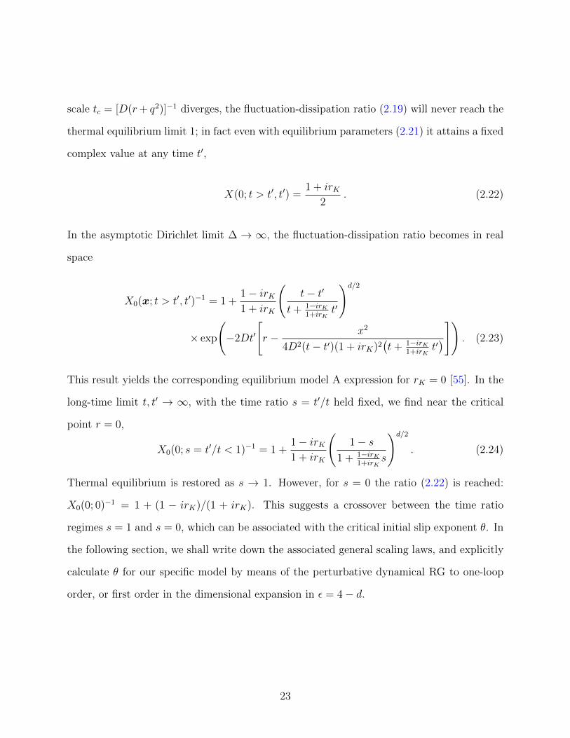
To first order in u′, the only contribution to Σ′ is the ‘Hartree loop’ shown in Fig. 2.2. In the
asymptotic limit ∆ → ∞, it is to be evaluated with the Dirichlet correlator (2.16), which
yields
Σ′(q, t) = δ(t)− 2
3u′D(1 + irU)G0
ψ∗ψ(q, t)
∫ddk
(2π)dCDψ∗ψ(k, t, t) . (2.31)
It is crucial to note that as the loop closes onto itself at intermediate time t′, the non-
equilibrium component in the first term of eq. (2.16) that contains r′ and rK disappears, and
the Dirichlet propagator contributions are identical to those in equilibrium. After straightfor-
ward temporal Fourier transform, we obtain after integration with dimensional regularization
(see appendix A):
Σ′(q, ω) = 1 +γu′(1 + irU)Ad
6[(1 + irU)r + (1 + irK)q2 + iω/D](d− 2)ε
× 1
[(3 + irU)r/2 + (1 + irK)q2/2 + iω/2D]1−d/2, (2.32)
where Ad = Γ(3− d/2)/2d−1πd/2.
26
q, 0 q, t
t'
k-k
P P
Figure 2.2: Feynman tadpole diagram or Hartree loop.
For the subsequent renormalization procedure, we set the normalization point to r = 0,
q = 0, but iω/2D = µ2 outside the infrared-singular region, whence in minimal subtraction
and with (2.21) and u = kBTu′:
Σ′(0, ω)NP = 1 +u(1 + irU)Adµ
−ε
3ε. (2.33)
Next we define the renormalization constant for the initial response field through ψR(x, 0) =
(Z0Zψ)1/2ψ(x, 0), whence Z0 absorbs the ultraviolet divergence in the renormalized self-
energy: Σ′R(q, ω) = Z1/20 Σ′(q, ω). Explicitly, we then find to one-loop order
Z0 = 1− 2uR(1 + irUR)
3ε+O(u2
R) , (2.34)
where uR = ZuuAdµ−ε and rUR = ZrU rU with Zu and ZrU determined in Ref. [5]. The
associated Wilson’s flow function that enters the renormalization group equation becomes
γ0(uR) = µ∂µ|0 lnZ0 =2
3uR(1 + irUR) +O(u2
R) . (2.35)
27

As a final step, one resorts to a short-time expansion for the response field ψ(x, t′) =
σ(t′)ψ(x, 0) + . . ., which through the RG flow translates into the asymptotic scaling σ(t′) =
(Dt′)−θσ(t′/ξz) [12], where we identify
θ = γ0(u∗)/2z . (2.36)
Under the RG flow, as stated before, rUR → 0 [5], and the non-linear coupling uR approaches
an infrared-stable fixed point u∗ = 3ε/5 + O(ε2) in dimensions d < dc = 4 (ε > 0). Thus
γ0(u∗) = 2ε/5+O(ε2), and with the standard two-loop critical exponents for the equilibrium
model A with two order parameter components [6, 29]
η = ε2/50 +O(ε3) , z = 2 + [6 ln(4/3)− 1 +O(ε)] η , (2.37)
we at last obtain
θ = ε/10 +O(ε2) , (2.38)
precisely as for the two-component model A.
2.4 Effect of two-loop and higher-order fluctuation cor-
rections
Higher-order loop corrections assuredly do not display the temporally local feature of the
tadpole graph, Fig. 2.2; hence non-equilibrium contributions and phase-coherent interference
terms from the dynamical correlation functions (2.15) cause deviations relative to the relax-
ation kinetics in the equilibrium model A. However, we know from the one-loop RG flow
equations that asymptotically all non-equilibrium parameters flow to zero [5]. Any effects
28

−20 −15 −10 −5 0ln(l)
0.0
0.1
0.2
0.3
0.4
0.5
0.6
0.7
u(l
)
∆(1) =0.01∆(1) =0.1∆(1) =1.0
−20 −15 −10 −5 0ln(l)
0.1
0.2
0.3
0.4
0.5
0.6
0.7
u(l
)
∆(1) =0.01∆(1) =0.1∆(1) =1.0
−20 −15 −10 −5 0ln(l)
0.60
0.65
0.70
0.75
0.80
0.85
0.90
0.95
1.00
u(l
)
∆(1) =0.01∆(1) =0.1∆(1) =1.0
(a) (b) (c)
Figure 2.3: Flow of the non-equilibrium parameter ∆(`) with initial values (a) ∆(1) = 0.01,(b) ∆(1) = 0.1, and (c) ∆(1) = 1.0 for several different initial values of the non-linearcoupling u(1) = 0.01, 0.1, 1.0, in d = 3 dimensions (ε = 1) and rk(1) = 1.0.
from the coherent quantum kinetics thus ultimately disappear at the critical point, which
also applies to the critical aging scaling regime. Yet for some initial values of the running
couplings, conceivably the RG flow might temporarily reach a transient metastable point
in parameter space, with associated dynamic scaling properties distinct from those of the
two-component model A.
In order to investigate this possibility, we consider the one-loop RG flow equations for the
running counterparts of the non-linear coupling uR and the non-equilibrium parameter ∆R =
rUR − rKR, as derived in Ref. [5]:
l∂lu(l) = u(l)
[−ε+
5
3u(l)− ∆(l)2
3[1 + rK(l)2]u(l) +O
(u(l)2
)],
l∂l∆(l) = ∆(l)
[1 +
2rK(l)∆(l) + ∆(l)2
1 + rK(l)2
]u(l)
3+O
(u(l)2
), (2.39)
obtained from the characteristics µ → µl. Their ultimately stable equilibrium fixed point
is ∆∗ = 0 and u∗ = 3ε/5 + O(ε2). We solve the coupled system of non-linear ordinary
differential equations (2.39) numerically by means of a four-step Runge-Kutta method, for
various initial values u(l = 1) and ∆(l = 1).
For dimensional parameter ε = 1, i.e., d = 3, the resulting RG flows of the coupling param-
29

−20 −15 −10 −5 0ln(l)
0.000
0.002
0.004
0.006
0.008
0.010
u(l
)
u(1) =0.01u(1) =0.1u(1) =1.0
−20 −15 −10 −5 0
ln(l)
0.00
0.02
0.04
0.06
0.08
0.10
0.12
u(l
)
u(1) =0.01u(1) =0.1u(1) =1.0
−20 −15 −10 −5 0
ln(l)
0.0
0.2
0.4
0.6
0.8
1.0
u(l
)
u(1) =0.01u(1) =0.1u(1) =1.0
(a) (b) (c)
Figure 2.4: Flow of the non-linear coupling parameter u(`) with initial values (a) u(1) = 0.01,(b) u(1) = 0.1, and (c) u(1) = 1.0 for several different initial values of the non-equilibriumparameter ∆(1) = 0.01, 0.1, 1.0, in d = 3 dimensions (ε = 1) and rk(1) = 1.0.
eters ∆(l) and u(l) are respectively shown in Figs. 2.3 and 2.4. We observe that the RG
flow quite quickly runs into the asymptotic values ∆∗ = 0 and u∗ = 3/5, which represents
the equilibrium model A fixed point. No interesting transient metastable crossover region is
discernible in these graphs for either parameter. This leads us to anticipate that the results
from two- or higher-loop fluctuation corrections ultimately become identical to the corre-
sponding ones for the two-component equilibrium model A [12], and no interesting distinct
crossover region emerges.
2.5 Spherical model
Our goal in this section is to analyze the partition function Z[h = 0] for an n-component
extension of the complex Landau–Ginzburg pseudo-Hamiltonian in the spherical model limit
n→∞, which can be directly generated from (2.5):
H[ψα] =
∫ddx
[(r + ir′)
n∑α=1
|ψα(x)|2 + (1 + irK)n∑
α=1
|∇ψα(x)|2
+u′
12(1 + irU)
(∑α
|ψα(x)|2)2 ]
. (2.40)
30

The corresponding spherical equilibrium model A has been investigated extensively in pre-
vious work, utilizing either a self-consistent decoupling method [12] or a Gaussian Hubbard–
Stratonovich transformation to effectively ‘linearize’ the quartic non-linear term in this
Hamiltonian (see, e.g., Refs. [6, 16, 70]). These two approaches are equivalent, but we
employ the latter to analyze our non-equilibrium system. To this end, we introduce an aux-
iliary field Ψ(x), through which the Gaussian Hubbard–Stratonovich transformation can be
performed, ∫d(iΨ) e−(1+irU )[Ψ(
∑α |ψα|2)−3Ψ2/u′] ∝ e−(1+irU )(
∑α |ψα|2)2/12 . (2.41)
Substituting this transformation as well as r′ = rKr, the augmented Hamiltonian becomes
H[ψα,Ψ] =
∫ddx
[(1 + irK)[r + Ψ(x)]
∑α
|ψα(x)|2 + (1 + irK)∑α
|∇ψα(x)|2
− 3
u′(1 + irU)Ψ(x)2
]. (2.42)
At this point the original order parameter fields can be integrated out, and one arrives at
Z[h = 0] ∝∫D[iΨ] exp
[3(1 + irU)
u′Ψ(x)2 − nTr ln
(1 + irK)GΨ(x,x′)−1
2π
], (2.43)
with the inverse Green’s function
GΨ(x,x′)−1 = [r + Ψ(x)−∇2] δ(x− x′) (2.44)
and its Fourier transform in momentum space
GΨ(q, q′)−1 = (r + q2) (2π)dδ(q + q′) + Ψ(q + q′) . (2.45)
Now recall that the RG fixed point for the non-linear coupling is u∗ ∝ ε/(n + 2); thus,
31

for large n, resetting the non-linear coupling as u = u′/n will render the parameter u′
independent of the number of components n as n → ∞. This yields the partition function
Z[h = 0] ∝∫D[iΨ]e−nΦ[Ψ] with the effective potential
Φ[Ψ] = −3(1 + irU)
u′
∫ddxΨ2(x) + Tr ln
(1 + irK)GΨ(x,x′)−1
2π. (2.46)
In the spherical model limit n→∞, the steepest-descent approximation will become exact,
that is we need to seek the solution of the classical field equation δΦ[Ψ]/Ψ(x) = 0. For
simplicity, we assume a homogeneous solution Ψ(x) = Ψ, whence the stationarity condition
yields a self-consistent equation for Ψ:
Ψ =u′
6(1 + irU)
∫ddq
(2π)d1
r + Ψ + q2. (2.47)
This result looks precisely like its equibilirium spherical model A counterpart, aside from the
overall complex prefactor 1+irU . Specifically, the integral is just the bare correlation function
C0(x = 0) with a shifted temperature parameter r → r+Ψ. Yet previous work [6] established
that asymptotically rU → 0 at the stable RG fixed point; therefore, one obtains the static
critical exponents of the equilibrium spherical model A: η = 0 and γ = 2ν = 2/(d − 2) for
d < dc = 4. Furthermore, the analysis for the dynamics of this non-equilibrium system will
also be essentially identical as for the equilibrium spherical model [6, 16], and results in the
dynamical critical and initial-slip exponents
z = 2 , θ = (4− d)/4 , (2.48)
both coinciding identical with the equilibrium spherical model A values.
The above analysis of the spherical model extension for the time-dependent complex Ginzburg–
32

Landau equation of course holds to all orders in a perturbative expansion. The fact that
the spherical model limit too recovers the equilibrium values for all critical exponents of this
system further supports our conclusion in the previous section 2.4 that higher-order fluctu-
ation corrections to the critical initial-slip exponent for our driven non-equilibrium kinetics
must be identical to those of model A in thermal equilibrium.
2.6 Conclusion and outlook
We have investigated the driven-dissipative non-equilibrium critical dynamics of a non-
conserved complex order parameter field. Specifically, we have addressed the situation where
the system experiences a sudden change in its parameters that quenches it from a random
initial configuration into the critical regime. We have mainly focused on the initial-slip crit-
ical exponent θ which governs the universal short-time behavior during the transient non-
equilibrium relaxation period before the asymptotic long-time stationary regime is reached.
We have employed the perturbative field-theoretical renormalization group method to cal-
culate the value of θ to first order in the dimensional ε expansion. Our explicit result turns
out identical to that for the equilibrium dynamical model A [12]. Quantum coherence effects
do not modify this universal scaling exponent owing to the temporal locality of the one-loop
Feynman diagram, or equivalently the fact that the phase term in the correlation propagator
is annihilated rendering the results identical to those for the equilibrium system without
drive. Rather than analytically calculating the complicated higher-order loop corrections,
we have invoked the one-loop renormalization group flow equations [5] as well as a suitable
spherical model extension, constructed along the lines of Ref. [70], to argue that the above
conclusion likely remains true to all orders in the perturbation expansion.
In the future, we intend to study this and related stochastic dynamical systems by means
33

of direct numerical integration. Comparing the resulting data with our analytical theory
should further aid our quantitative understanding of the dynamical critical properties of
driven-dissipative quantum systems that experience parameter quenches, and hence take
us another step closer towards the ultimate goal of obtaining a complete and systematic
classification of non-equilibrium dynamical criticality.
Appendix. Dimensional regularization, Feynman
parametrization
In order to arrive at a small expansion parameter for the perturbational analysis in our field-
theoretic RG approach, we need to consider non-integer spatial dimensions close and below
the upper critical dimension dc = 4. We may consider these non-integer dimensionalities
as an analytical continuation of integer ones by means of dimensional regularization. The
fluctuation loop integrals in momentum space associated with the Feynman diagrams are
tpyically of the following form (see, e.g., Ref. [6]):
I(σ,s)d (τ) =
∫ddk
(2π)dk2σ
(τ + k2)s=
Γ(σ + d/2)Γ(s− σ − d/2)
2dπd/2Γ(d/2)Γ(s)τσ−s+d/2 . (2.49)
Integrals with different denominators can be reduced to this form through Feynman’s parametriza-
tion:
1
ArBs=
Γ(r + s)
Γ(r)Γ(s)
∫ 1
0
xr−1(1− x)s−1
[xA+ (1− x)B]r+sdx . (2.50)
These expressions are widely used to evaluate the momentum loop integrals. Euler’s gamma
function provides the appropriate interpolation for non-integer dimensions.
34

Chapter 3
Aging phenomena in the
two-dimensional complex
Ginzburg-Landau equation
3.1 Introduction
Systems can be brought out of equilibrium states through a rapid change of their thermo-
dynamic control parameter(s). If strong fluctuation effects are subsequently generated and
govern the relaxation processes, they cannot rapidly return to the stationary states, espe-
cially in the continuous transition case or at the critical point where the typical relaxation
time scales diverge. “Aging phenomena,” which describe the change of materials properties
over time with or without an applied external force, will emerge when this significant slowing-
down present [16]. These phenomena are important in physics studies since they provide the
probabilities to predict long-time behavior according to the thermal history of associated
systems. In these systems time-translation-invariance is spontaneously broken due to the
35

fact that a specified time is chosen to kick the systems out of its equilibrium state, which is
usually at t = 0.0. Concurrently, a dynamical scaling is also suggested underlying this slow
relaxation processes. Thus, a general definition of aging phenomena is given as: physical
aging can be observed in a many-body system when its relaxation process satisfies three
properties [16]: the relaxation process is slow, i. e. non-exponential relaxation; the breaking
of time-translation-invariance; and dynamical scaling is observed. Furthermore, another un-
expected property of aging phenomena is that physical aging is also thermoreversible even
though the time-translation-invariance is broken, which enhances the importance as better
understanding these phenomena.
Two-time quantities are often employed to characterize aging phenomena. For example, the
two-time autocorrelation function
C(t, s) = 〈φ(t)φ(s)〉. (3.1)
Here φ(t) generally is the time-dependent order parameter. t is the observation time, and s is
called waiting time, which must be earlier than t due to causality. To ensure the emergence
of dynamical scaling, we require t � s � t0, where t0 referred to as any microscopic time
scale. We may expect C(t, s) to follow a simple aging scaling form if aging phenomena is
observed:
C(t, s) = s−bfC(t/s), (3.2)
where b is the aging exponent and fC(y) is the scaling function which only depends on the
ratio y = t/s.
Aging phenomena[16] are known to exist in a broad variety of physical systems, such as Ising
model [74, 75], population dynamics models [65], and systems of skyrmions [76]. However,
most of the examples we mentioned here are investigating these phenomena using Monte
36

Carlo simulations or molecular dynamics simulations. A numerical exploration of this topic
in fieldtheoretic regime is important to better understand these systems.
To fulfill this objective, we study the complex Ginzburg-Landau (CGL) equation in this
paper. The CGL is one of the most studied nonlinear partial differential equations in the
physics community. It is thought to be at least a natural description of the kernel of many
physical systems that can be characterized by an amplitude (or ”envelope” or ”modula-
tional”) equation. It includes only a simplest cubic nonlinear term; however, it describes a
large number of phenomena, spread from nonlinear waves to second-order phase transitions
to Bose-Einstein condensation to liquid crystals.
According to the vast library of previous work, a reduced form of the original CGL equation
can be obtained through rescaling, and is usually employed in the relevant numerical study.
It is
∂tA(x, t) = A(x, t) + (1 + iα)∇2A(x, t)
−(1 + iβ)|A(x, t)|2A(x, t). (3.3)
Here, the A(x, t) is a complex field, while α and β are two real parameters characterize the
linear and non-linear dispersion, respectively. Eq. (3.3) is an amplitude equation of Hopf
bifurcation in the spatially homogeneous case. In the spatially extended case, especially in
two dimensions, it will express rich behaviors, including spatio-temporal chaos[77], nucleation
of spiral wave structures [78] and dynamic freezing [79]. Therefore, it is reasonable to expect
aging phenomena to take place in this kind of system. Chate and Manneville have pointed
out that it is promising to investigate aging in the frozen state of two-dimensional CGL[80];
however, there are actually various problems in the observation of aging behavior in most of
the states of two-dimensional CGL systems, which we will discuss in details.
37
3.2 Model description
First of all, in two-dimensional CGL, the strongly fluctuating turbulent states, either with
or without topological defects, are hopeless for observing aging, as they are both strong
disordering states. Topological defects, specify in two dimensions, are identified by the zeros
of the complex field A(x, t). At these points there is singularity of the phase θ = argA(x, t),
since they can not be defined in the case of zero amplitude. The so-called topological charge
n = 1/(2π)∮Cdθ is used to quantify this singularities, where C is a contour around the zero
of A(x, t). Only single-charge defects, with n = ±1, are topologically stable. They can emit
stable and well-established spiral waves, which will fill the whole space and make the systems
frozen. The relaxation processes of these frozen states, on another hand, is too fast for aging
phenomena to be found, which we numerically verify.
However, there is a connection between CGL systems and aging phenomena. It is reported
that there aging has been observed in two-dimensional XY models[81]. Indeed, in the special
case of α = β = 0.0, Eq. (3.3) can be reduced to the “real” Ginzburg-Landau (RGL) equa-
tion, which describes kinetics resembling the model E for a nonconserved two component
order parameter field, namely, the classical two-dimensional XY model[5]. Dynamics of the
defects, which actually become vortices, in the real Ginzburg-Landau systems are analogous
to charge point. Two oppositely charged topological defects will accelerate towards each
other and eventually the attraction will lead to the annihilation of both defects. Similar
dynamics should be expected for the CGL case. However, in the frozen state, the surviv-
ing topological defects can not interact with each other due to the fact that there are shock
structures between different well-established spiral domains. Information is then screened by
these shocks and hence no interaction exists between defects in different domains. Therefore,
to ensure further slow dynamics, one should try to further destroy these shocks. Das[79] had
proposed to introduce disorder in either the α or β parameters to unlock the frozen dynam-
38

ics. However, this strategy will result in more complicated behavior for the characteristic
length of the CGL system. It divides into two significant different sections, the first one
corresponds to the transient freezing stage, and the second part is suggested to be consistent
with exponential behavior. Thus this strategy actually fails to provide us aging behavior.
An interesting fact we notice is that in the previous study from the same group[82] , power
law behavior of the characteristic length evolution was observed when one fixed α = 0.0
and set β = 0.25 or 0.5. Aging phenomena can be expected at these points. According to
their own suggestion, this is due to the fact that the average length scale L(t) of a single
spiral structure is comparable to the wavelength of the associated asymptotic plane wave
solution of those spiral waves. Spirals will then behave similarly to those vortices seen in the
XY model. This condition will be satisfied either when approaching the “real” Ginzburg-
Landau limit in the “focusing-quadrants” where αβ < 0.0 and the spirals are focusing, or
when a system is quenched into the “defocusing-quadrant” where αβ > 0.0, and the spiral
wave are defocusing. Bohr et al.[11] study the spiral-domain patterns and shocks structures,
and also suggest that if the length scale of a single spiral structure is not much larger than
the characteristic wavelength, the phase matching constraint may be broken down and no
well-established shock lines will be formed.
We study the aging behavior of the two-dimensional complex Ginzburg-Landau equation for
both cases respectively, which are distinguished by the winding behavior of related spirals.
We extract the dynamic exponent z, which indicates the scaling behavior as L(t) ∼ t1/z as
well as the corresponding aging exponents of aging phenomena for all the parameter choices
we tested. We also try to calculate the autocorrelation exponent λC from the scaling function
fc(y) ∼ y−λC/z for the “focusing” spiral case. We do not repeat this step for the “defocusing”
case as there is observable bending in the resulting curves for scaled two-time autocorrela-
tions. We claim that our estimate of λC may not be very reliable. However, as systems
39

are approaching the XY model for this case, this exponent will provide us probabilities for
further comparison of these two models.
3.3 Numerical scheme
We employ standard Euler discretization method to solve Eq. (3.3), with a forward finite
differential for time and a central differential for the ∇2. We will focus on systems on
two-dimensional square lattices with periodic boundary conditions. Our system size will be
512× 512 and the grid sizes are ∆x = 1, ∆t = 0.002, unless otherwise mentioned. However,
we have also tested other system sizes and the ∆t = 0.001 case, which will provide us
consistent results here. We will always use entirely random initial configurations to ensuring
that we have enough topological defects at the very beginning. We also add a small Gaussian,
white, and Markovian noise term λη(x, t) into Eq. (3.3) to make it Langevin like. λ = 0.1
is the noise strength and η(x, t) can be characterized by these correlators:
〈η(x, t)〉 = 〈η∗(x, t)〉 = 0,
〈η∗(x, t)η(x′, t′)〉 = γ2δ(x− x′)δ(t− t′),
〈η(x, t)η(x′, t′)〉 = 〈η∗(x, t)η∗(x′, t′)〉 = 0, (3.4)
with γ = 0.2 and η∗(x, t) as the complex conjugate of η(x, t).
The characteristic length of system is thought to be the average size of spiral domains and
can be calculated as:
l(t) =L√N(t)
. (3.5)
Here L = 512 is the linear size of our system and N(t) is the total number of topological
defects in the system at time t. To investigate the aging phenomena, we also need to calculate
40

0 100 200 300 400 500
0
100
200
300
400
500
Amplitude
0 100 200 300 400 500
0
100
200
300
400
500
Phase
−1.2
−0.8
−0.4
0.0
0.4
0.8
1.2
0.1
0.2
0.3
0.4
0.5
0.6
0.7
0.8
0.9
1.0
Figure 3.1: An example system configuration obtained from the solution of CGL on a two-dimensional square lattice for the focusing spiral wave case when quenched near the RGLlimit with α = −0.05; β = 0.5 and t = 500. The white-red plot (on the left) shows theamplitude of the complex order parameter; the blue-white one depicts the phase.
the two time autocorrelation function. However, since we are working with complex order
parameter, we need to modify Eq. (3.1). We will estimate the modulus of this complex
function as follow:
C(t, s) = |〈A(x, t)A∗(x, s)〉|. (3.6)
A∗(x, t) is the complex conjugate of A(x, t). Without ambiguity, this is what we refer to as
the two-time autocorrelation function in rest of this letter.
3.4 Results
We consider both the focusing spiral wave case when systems are quenched near the RGL
limit and the defocusing spiral wave case. Fig. 3.1 shows example plots of system configura-
tions for the focusing case. In the phase plot (blue-while one, or right one), there are small
41

spiral structures which are not well-established due to the fact their wavelength is comparable
to their average size, and hence there will be no significant shock structures in the amplitude
plot (red-white one, or left one). Most of the space in the amplitude plot holds an amplitude
around |A(x, t)| = 1.0 except for those deep red points which are topological defects cores
with zero amplitude. There is no spontaneous creation of defect pairs in this case. They just
try to approach the nearest neighbor with opposite topological charge and annihilate with
each other. Due to this, there are spiral waves in the phase plot. When the distance between
two oppositely charged defects are close enough, instead of directly approaching like vortices
in the XY model, they tend to drift along the tangential direction, and merge gradually and
eventually annihilate. Some residual of the shocks can be viewed in the amplitude plot as
the bright still regions that indicate |A(x, t)| > 1.0. These residual, will become prominent
when departing from the RGL limit and will finally partition systems into clearly separated
domains. The dynamics will become freezing in this case. Defects with defocusing spiral will
behave similarly to the focusing case, except the spirals rotate differently.
As shown in Fig. 3.2 (a), there is suggestive scaling behavior of the characteristic length of
the CGL system with control parameter pair (α, β) = (−0.05, 0.5) if the strong fluctuating
part due to the finite size effect is ignored. A dynamic exponent 1/z = 0.307 can be extracted.
It is relatively smaller than the value 1/z = 0.5, which is obtained in the two-dimensional
XY model below the critical temperature and quenched from a totally disordered initial
state[74]. A logarithmic correction in the relation between the characteristic length and the
time, l(t) ∼ (t/ ln t)1/z is also acquired in the latter case. However, if we also apply this
logarithmic correction in our CGL case, the resulted scaling behavior of the characteristic
length is even worse than the no correction case with an aging exponent b ∼ 0.8 and the
autocorrelation exponent λC/z = 1.49. Again compared with the XY model [81] where
b = 0.03 and λC/z = 1.05 when T/Tc = 0.3, both our aging exponent b and auto-correlation
42

0.5 1.0 1.5 2.0 2.5 3.0 3.5log10(t)
−0.2
0.0
0.2
0.4
0.6
dlo
g 10[L
(t)]/d
log 1
0(t)
dlog10[L(t)]dlog10(t)
= 0.307
Data
−0.2 0.0 0.2 0.4 0.6 0.8 1.0 1.2 1.4 1.6log10(t/s)
0.0
0.5
1.0
1.5
2.0
log 1
0(sb
C),
b=
0.8
s=140.0s=170.0s=200.0s=230.0
(a) (b)
Figure 3.2: (a) The derivative of the logarithm of the characteristic length of the two-dimensional CGL system with respect to the logarithm of the time, with control parametersα = −0.05; β = 0.5, namely for focusing spirals. (b) the scaled two-time autocorrelationfunction for various waiting time s. The aging exponent here is b = 0.8. The blue dashed linewith slope 1.49 is roughly parallel to the collapsed curve, which indicates the autocorrelationexponent λC/z = −1.49. The data result from averaging over 1000 independent runs.
exponent λC are larger. All these facts suggest that the scaling and aging behavior of the
CGL systems with nonvanishing control parameter pair (b, c) is clearly different from the
classic XY model. We then try to vary the control parameter pair (b, c) to reinforce our
conclusions. Relevant results are listed in Table 3.1. We use 1000 independent realizations
for each parameter pairs. We only try to extract the autocorrelation exponent when we think
we see a meaningful value, namely when the scaled autocorrelation function looks linear.
Table 3.1: Measured values of the dynamic, aging scaling, and autocorrelation exponents forthe focusing spiral case
(α, β) 1/z b λC/z
(−0.05, 0.5) 0.307± 0.003 [0.69, 0.80] 1.49± 0.02(−0.05, 0.4) 0.354± 0.003 N/A N/A(−0.05, 0.6) 0.293± 0.004 [0.35, 0.44] 1.22± 0.01(−0.04, 0.5) 0.312± 0.003 [0.72, 0.85] 1.42± 0.02(−0.06, 0.5) 0.298± 0.004 [0.63, 0.77] 1.45± 0.01
43

0.5 1.0 1.5 2.0 2.5 3.0 3.5log10(t)
−0.2
0.0
0.2
0.4
0.6
dlo
g 10[L
(t)]/d
log 1
0(t)
dlog10[L(t)]dlog10(t)
= 0.431
Data
−0.2 0.0 0.2 0.4 0.6 0.8 1.0 1.2 1.4 1.6log10(t/s)
−0.2
0.0
0.2
0.4
0.6
log 1
0(sb
C),
b=
0.25
s=140.0s=170.0s=200.0s=230.0
(a) (b)
Figure 3.3: (a) The derivative of the logarithm of the characteristic length of the two-dimensional CGL system with respect to the logarithm of the time, with control parametersα = 1.176; β = 0.7, namely for defocusing spirals. (b) the scaled two-time autocorrelationfunction for various waiting times s. The aging exponent here is b = 0.25. These resultswere obtained by averaging over 8000 independent runs.
Here we focused ourselves the small α case, as it can be directly related to the spatial scale.
According to the extracted values of the aging exponent b, we conclude that these suggest a
non-universal behavior of our CGL systems with focusing spirals. This is reasonable since the
non-vanishing linear term in Eq. (3.3) automatically assumes that we are below the critical
point here. The variance is stronger when we change the parameter β in this small α case,
while only slightly changing if we change α. This is because β contributes much more than
α to the deviation from the RGL limit α = β = 0.0. Furthermore, the (−0.05, 0.6) systems
become almost frozen at the very end. The scaled two-time autocorrelation functions curves
are observed to be dispersed in this parameter choice. On the other hand, the (−0.05, 0.4)
systems show no significant aging scaling behavior during the time regime we observe. This
absence of aging phenomena can be viewed as more evidence of non-universal behavior.
Aside from the small α case in the focusing spiral quadrant, which is considered to explicitly
approach the RGL limit, one can also eliminate the significant shock structures and have
interactive spiral dynamics through quenching the systems into the defocusing quadrant,
44
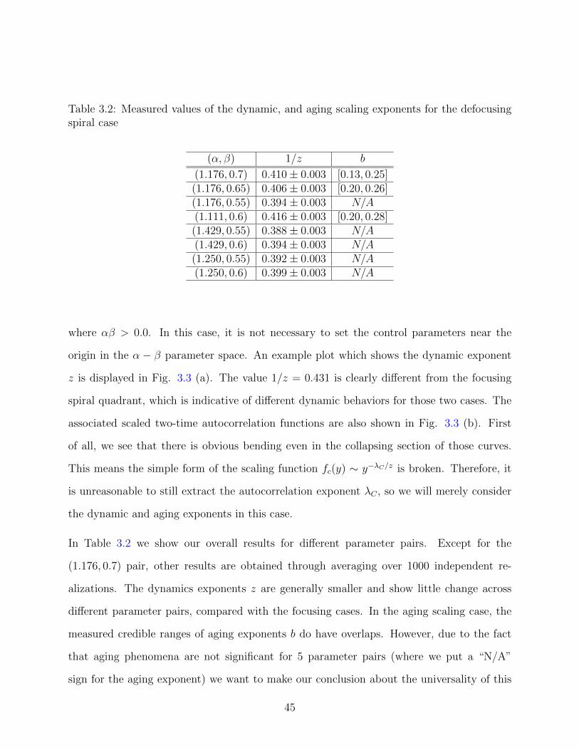
Table 3.2: Measured values of the dynamic, and aging scaling exponents for the defocusingspiral case
(α, β) 1/z b
(1.176, 0.7) 0.410± 0.003 [0.13, 0.25](1.176, 0.65) 0.406± 0.003 [0.20, 0.26](1.176, 0.55) 0.394± 0.003 N/A(1.111, 0.6) 0.416± 0.003 [0.20, 0.28](1.429, 0.55) 0.388± 0.003 N/A(1.429, 0.6) 0.394± 0.003 N/A(1.250, 0.55) 0.392± 0.003 N/A(1.250, 0.6) 0.399± 0.003 N/A
where αβ > 0.0. In this case, it is not necessary to set the control parameters near the
origin in the α − β parameter space. An example plot which shows the dynamic exponent
z is displayed in Fig. 3.3 (a). The value 1/z = 0.431 is clearly different from the focusing
spiral quadrant, which is indicative of different dynamic behaviors for those two cases. The
associated scaled two-time autocorrelation functions are also shown in Fig. 3.3 (b). First
of all, we see that there is obvious bending even in the collapsing section of those curves.
This means the simple form of the scaling function fc(y) ∼ y−λC/z is broken. Therefore, it
is unreasonable to still extract the autocorrelation exponent λC , so we will merely consider
the dynamic and aging exponents in this case.
In Table 3.2 we show our overall results for different parameter pairs. Except for the
(1.176, 0.7) pair, other results are obtained through averaging over 1000 independent re-
alizations. The dynamics exponents z are generally smaller and show little change across
different parameter pairs, compared with the focusing cases. In the aging scaling case, the
measured credible ranges of aging exponents b do have overlaps. However, due to the fact
that aging phenomena are not significant for 5 parameter pairs (where we put a “N/A”
sign for the aging exponent) we want to make our conclusion about the universality of this
45

exponent more carefully. To this end, we want to first answer the question of why dynamical
scaling behavior can generally exist and why spirals can behave like vortices even in systems
that are quenched far from the RGL limit α = β = 0. In fact, there exists a more general
case for Eq. (3.3) other than the RGL limit, which is obtained by setting α = β 6= 0. This
special case can be related to the RGL limit through a transformation into a “rotating” frame
A → A exp(ibt) if one is going to obtain an approximately analytic solution of Eq. (3.3)
for the isolated spiral case[7]. After neglecting high-order corrections, the resulting solution
is identical with the RGL solution except for a shift in the wavenumber. In other words,
there exists a whole branch of vortices-like behavior limit in the defocusing quadrant, which
is not the case when αβ < 0.0. Systems that are quenched far from the origin in (α−β) pa-
rameter space in defocusing quadrant can still show nice dynamical scaling and aging when
their control parameter pair is set near the line α = β. This fact, as well as our numerical
results in Table 3.2, suggest that the criterion for significant aging phenomena emerging or
not is that aging scaling is restored when the control parameter pairs approaching the limit
α− β → 0. The asymptotic wavenumber of the spiral vanishes in this limit. Therefore, the
effect of shock structures is assumed to be weak here. However, due to the fact that when
α = β 6= 0 there is still an obvious rotation of the equiphase lines, the interaction between
defects is expected to be oblique repulsion and attraction. Two defects will never approach
each along the line connecting them, like the vortices in RGL case. They will either spiral
with respect to each other if they are like-charged, or move along the tangential direction,
or approach each gradually and finally annihilate with each other in the oppositely charged
case.
We then further test this criterion by explicitly quenching the control parameter near the
α = β limit and shows our results in Table 3.3.
Firstly, the result of aging exponent b = 0.03 from previous study of the two-dimensional
46

Table 3.3: Measured values of the dynamic and aging scaling exponents for the defocusingspiral case, near the limit α = β
(α, β) 1/z b
(1.2, 1.2) 0.441± 0.002 [0.00, 0.13](1.0, 1.0) 0.426± 0.003 [0.00, 0.13](1.2, 1.25) 0.444± 0.002 [0.00, 0.15](1.2, 1.15) 0.440± 0.003 [0.00, 0.13]
XY model below the critical temperature[81] falls into all the extracted credible ranges of b
in these tests. This confirm the analytic conclusion that CGL will restore some XY model
behaviors when approaching the α = β 6= 0. The dynamical scaling exponent z is also
observed to be closer to the limit 1/z = 0.5 than that in Table 3.1 and Table 3.2. The
remaining deviation can be either from the fact that CGL still holds different dynamical
scaling behavior from the XY model, or from the logarithmic correction issue. Further
studies are needed to confirm these effects. And finally, although these aging exponents
share similar ranges in Table 3.3, they are clearly different from those in Table 3.2, which
will also suggest a non-universal behavior of the spirals in the defocusing quadrant. Aside
from that, the slightly bending features persist even if we are in the limit case α = β. We
may tentatively suggest that this is because the equiphase lines of the resulted spirals (or
vortices) are defocusing rotating, which will definitely affect the dynamics of those spirals.
3.5 Conclusion
In summary, we have investigated the dynamic scaling and aging phenomena in the two-
dimensional CGL equation, both in the focusing and defocusing spiral quadrants. To avoid
the shock structures which will prevent the interaction between defects and cause the systems
to become frozen, we should quench the control parameters near the RGL limit α = β = 0.0
47

in the focusing spiral case or be in the defocusing quadrant. In the time regime we considered
here, both the dynamical scaling and aging are slightly different from the vortices behavior in
the two-dimensional XY model when quenched below the critical temperature in the focusing
spiral systems, even if they are considered to be approaching to that limit. In fact, the aging
phenomena will even turn out to be absent for some control parameter pairs, serving as
evidence that there exist non-universal scaling behavior in these systems. In the defocusing
spiral case, as one can approach another limit case α = β while not having to be near the
regime of α = β = 0, aging phenomena can still be restored even if systems are quenched
far away from the origin in the parameter space. This non-universal behavior is suggested
again by our observations. A slightly bending of the scaled two-time autocorrelation function
curves is always found in all the defocusing spiral cases, whether the aging scaling behaviour
emerges or not. We tentatively assumed that this can be viewed as an effect of the defocusing
rotation of the equiphase lines connecting different topological defects(or vortices). Thus, no
simple aging scaling exists in this defocusing spiral quadrant. Better statistical data, as well
as larger system sizes, are needed to further confirm those conclusions. Different boundary
conditions, and other initial configurations, e. g. uniform initial configurations with slight
perturbations may also be important here since the scaling behavior of these systems is
non-universal.
48
Chapter 4
Nucleation of spatio-temporal
structures from defect turbulence in
the two-dimensional complex
Ginzburg–Landau equation
4.1 Introduction
Spontaneous spatial structure formation, as well as its inverse process, the dynamical de-
struction of patterns through spatio-temporal chaos, are of considerable interest, especially
in far-from-equilibrium systems. These phenomena are encountered in condensed matter
physics, chemistry, and biology. Studies of this topic have benefited from the recent devel-
opment of careful experiments, as well as analytic and numerical tools. Non-equilibrium
spatial patterns often emerge due to linear system instabilities that are induced by varying
49

some control parameter(s) beyond certain thresholds [50, 51]. The term “ideal pattern” is
defined to represent the spatially periodic structure of an infinitely extended system. De-
fects, which can generally be viewed as any departure from this ideal pattern, constitute
important “real pattern” effects. Their structures may reflect the topological characteristics
of the ideal patterns in a (quasi-)stationary dynamical state. For example, the stationary
kinetics in non-equilibrium steady states as well as the relaxation towards such station-
ary regimes are often governed by the properties of topological defects in these non-linear
dynamical systems. Indeed, the onset of spatio-temporal chaos in excitable or oscillatory
media can trigger the appearance of topological defects, which are point-like objects in two
dimensions, but can be extended in higher dimensions. A striking example are the famous
chemical oscillations in the Belousov–Zhabotinsky (BZ) reactions [83–87], where the defect
points emit spiral chemical waves. Such striking wave patterns are also observed in spatially
extended stochastic population dynamics, e.g., the stochastic May–Leonard model with three
cyclically competing species [88–91]. Other types of topological defects are encountered in
driven systems maintaining non-linear traveling waves such as Rayleigh–Benard convection
in planar nematic liquid crystals [92, 93], or electroconvecting nematic liquid crystals [94].
Here the defects constitute dislocations in the roll pattern of the traveling waves [95].
A simple, generic description of many pattern-forming systems is afforded through the com-
plex Ginzburg–Landau equation (CGL). Indeed, the CGL is considered to at least represent
the “kernel” of many amplitude equation models [80] that have been employed to character-
ize spontaneous spatial pattern formation [95, 96]. A large number of numerical studies of
the CGL in two dimensions has been performed over the past three decades, and uncovered
a wide variety of intriguing dynamical behavior upon varying certain control parameters. In
this work, we mostly consider the transition from the “defect-mediated turbulence” state
with strong spatio-temporal fluctuations to the so-called “frozen” state displaying beautiful
50

stationary spiral wave patterns that resemble structures observed in two-dimensional oscil-
lating media (e.g., the BZ reactions and the stochastic May–Leonard model). Only a few
previous studies have addressed the transition dynamics between these two states, namely
the crossover from the strongly fluctuating into a dynamically frozen state [78]. This pro-
cess is thought to be important for controlling spatio-temporal chaos in spatially extended
systems [97, 98]. The inverse transition has been also observed in a real BZ reaction with
an open reactor [99]. The transition between turbulent and frozen spiral states can be al-
tered by adding a chiral symmetry breaking term into the right-hand-side of the CGL [100],
which also modifies the specific form of the dynamical equation and hence the phase dia-
gram. To obtain a better understanding of the accompanying transient processes, we aim for
a quantitative characterization of the transition dynamics, where one switches the control
parameters beyond a transition limit in parameter space. The defect-mediated turbulence
state is thus rendered meta-stable, and well-established spiral structures emerge. As pointed
out in Ref. [78], when turbulence becomes transient, the onset of the formation of spiral
wave structures can be viewed as a nucleation process. The authors of Ref. [78] primarily
investigated situations where the control parameters were chosen near the crossover regime,
and hence the defect-mediated turbulence state becomes just unstable. In the present study,
we conversely also consider sudden parameter switches which represent deep quenches into
the stable frozen state regime. Based on our numerical results and subsequent finite-size
extrapolation analysis, we obtain evidence for a non-vanishing nucleation barrier for the for-
mation of spiral structures. Consequently we conclude that the transition from the defect
turbulence to the quasi-stationary frozen state is of a discontinuous nature.
In addition to spiral wave structures, reaction-diffusion systems may also exhibit “target wave
patterns” in the presence of spatial inhomogeneities. For example, the BZ reaction supports
target waves if a dust grain or other impurity is inserted [83, 85]. According to Refs. [101,
51

102], a pacemaker is needed to stabilize the resulting wave pattern. However, target patterns
can also emerge in a homogeneous system if it is subjected to perturbations with oscillating
concentrations [101–104]. The singularity point in the defect center will assume this trigger
role for stable spiral structures, whence spontaneous creation and annihilation of defect pairs
may occur. Those pacemakers or nucleation centers ensure that the internal regions of those
heterogeneous nuclei will maintain an effectively higher oscillation frequency than the outside
bulk of the oscillatory medium, which is the reason why a local inhomogeneity is needed to
generate target waves. However, in contrast to rotating spirals, target waves take a concentric
circular shape, and propagate radially outward from their source. Previous work indicated
that target waves are characterized by a vanishing topological charge [105], in distinction to
the positively or negatively charged (oriented) spirals. There are also intriguing studies of
spatiotemporal chaos control through target waves [106]. Thus, in this work we also study
target wave nucleation and compare this scenario with the aforementioned spiral droplet
nucleation.
This paper is structured as follows: A general review of the CGL model is presented in
section 4.2; section 4.3 describes our numerical scheme as well as the methodology we devised
to characterize the spatial scale of the CGL system, especially when it contains “droplet”
nucleating structures, and to determine the nucleation time distribution. In section 4.4,
we implement our algorithm and numerical analysis to study spontaneous spiral droplet
nucleation events in two-dimensional CGL systems subject to two distinct quench protocols:
namely either from fully randomized initial conditions, or from initial configurations that
correspond to stationary states in the defect turbulence region. Target wave nucleation with
an artificially prepared pacemaker are investigated and analyzed in section 4.5. Finally, we
summarize our results in the concluding section 4.6.
52

4.2 Model Description
A general description of non-linear driven-dissipative systems is afforded by the complex
Ginzburg–Landau equation in terms of a complex field A(x, t) [107–109]. A(x, t) provides
the amplitude and phase of the lowest Fourier mode of a characteristic quantity C(x, t)
describing the system. Therefore, C(x, t) can be decomposed as:
C(x, t) = C0 + A(x, t)eiω0t + c.c.+ h.o.t., (4.1)
where C0 is a constant, c.c. means complex conjugation, and h.o.t. denotes higher-order
terms. Furthermore, compared with the frequency scale ω0, the complex field A(x, t) is
assumed to be slowly varying. A(x, t) is often called order parameter, and obeys the CGL
which can be written in a rescaled form:
∂tA(x, t) = A(x, t) + (1 + ib)∇2A(x, t)
−(1 + ic)|A(x, t)|2A(x, t), (4.2)
with real constants b and c that characterize the linear and non-linear dispersion, respec-
tively. Here, the parameters that describe the deviation from the transition threshold, the
diffusivity, and the non-linear saturation have been rescaled to 1. Note that the frequency
shift (the imaginary part of the coefficient of the linear term) is eliminated by gauge symme-
try. Eq. (4.2) is invariant under the transformation (A, b, c) → (A∗,−b,−c) [7]. Therefore,
we only need to consider half of the parameter space in the b-c plane and can directly pre-
dict same behavior of the system from this mapping; for example, in the two-dimensional
(b, c) parameter space, the first and third quadrants are equivalent due to that invariance
transformation. The first and third quadrants are labeled “defocusing quadrants”, since the
53
associated spiral waves rotate along the same direction as the equi-phase lines (or spiral
arms). The second and fourth quadrants are correspondingly called “focusing quadrants”,
and yield spirals that rotate inversely with respect to the defocusing quadrants. We shall
restrict ourselves to the focusing case in this paper.
The CGL (4.2) describes spatially extended systems whose homogeneous state is oscillatory
around the threshold of a super-critical Hopf bifurcation, e.g., for which the stable stationary
dynamical state becomes a global limit cycle. The isotropic non-linear partial differential
equation (4.2) reduces to the “real” Ginzburg-Landau Equation (GL) for b = c = 0. It may
also be viewed as a disspative extension of the conservative non-linear Schrodinger equation
[7], which formally follows in the limits b, c→∞ in Eq. (4.2).
There exists a simple homogeneous solution of Eq. (4.2), namely A = exp(−ict + φ) with
frequency ω = c and an arbitrary constant phase φ. This spatially uniform periodic solution
becomes unstable when 1 + bc < 0, known as the Benjamin–Feir limit. Long-wavelength
modes with wave numbers below a critical threshold proportional to√|1 + bc| will then be
exponentially enhanced. A more general solution form is a family of traveling plane wave
solutions,
A(x, t) =√
1−Q2 ei(Q·x−ωt), (4.3)
with frequency ω = c+(b−c)Q2, restricted to Q2 < 1. The homogeneous oscillating solution
is restored in the limit Q→ 0. The stability of this solution can be tested through perturbing
the plane wave solution (4.3) with modulation modes and studying their complex growth
rate [7, 110, 111]. Restricting the analysis to the most dangerous longitudinal perturbation
and performing a long-wavelength expansion (with b 6= c and Q 6= 0), one arrives at the
Eckhaus criterion for the plane wave solution (4.3) that can be tested against convective
instability for non-zero group velocities [112–114], for which the initial localized perturbation
will be amplified. However, at fixed position, it can in fact not be amplified due to the drift
54
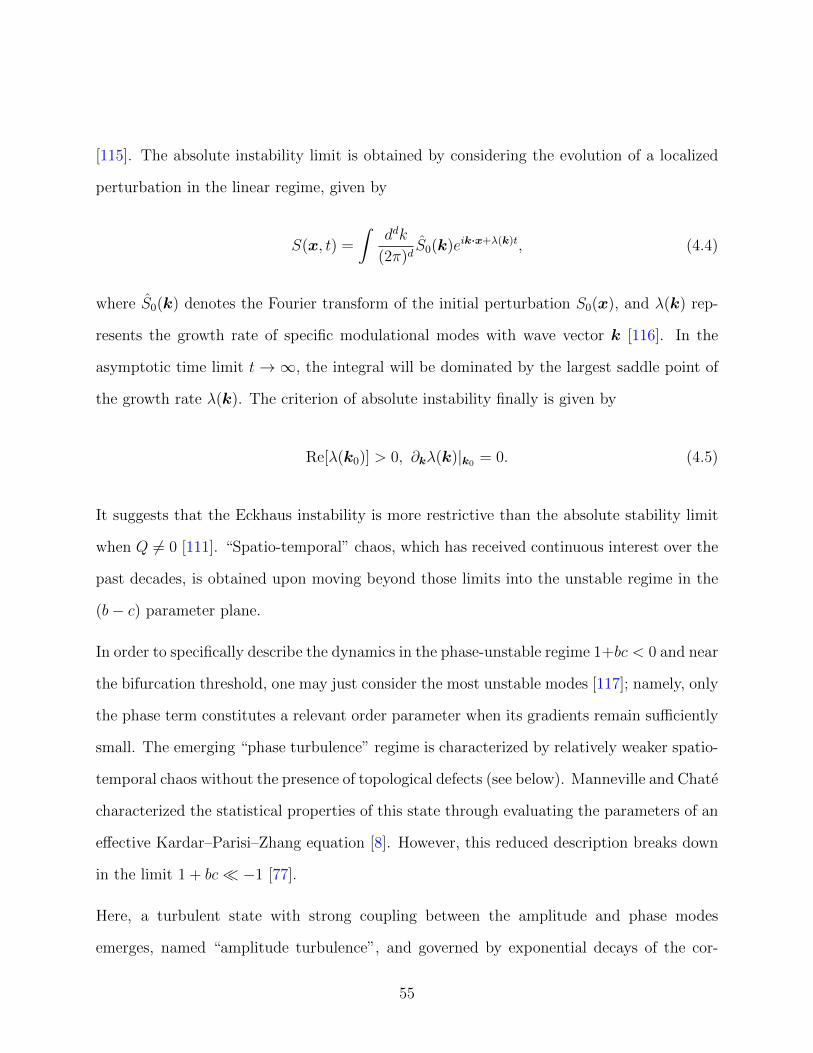
[115]. The absolute instability limit is obtained by considering the evolution of a localized
perturbation in the linear regime, given by
S(x, t) =
∫ddk
(2π)dS0(k)eik·x+λ(k)t, (4.4)
where S0(k) denotes the Fourier transform of the initial perturbation S0(x), and λ(k) rep-
resents the growth rate of specific modulational modes with wave vector k [116]. In the
asymptotic time limit t→∞, the integral will be dominated by the largest saddle point of
the growth rate λ(k). The criterion of absolute instability finally is given by
Re[λ(k0)] > 0, ∂kλ(k)|k0 = 0. (4.5)
It suggests that the Eckhaus instability is more restrictive than the absolute stability limit
when Q 6= 0 [111]. “Spatio-temporal” chaos, which has received continuous interest over the
past decades, is obtained upon moving beyond those limits into the unstable regime in the
(b− c) parameter plane.
In order to specifically describe the dynamics in the phase-unstable regime 1+bc < 0 and near
the bifurcation threshold, one may just consider the most unstable modes [117]; namely, only
the phase term constitutes a relevant order parameter when its gradients remain sufficiently
small. The emerging “phase turbulence” regime is characterized by relatively weaker spatio-
temporal chaos without the presence of topological defects (see below). Manneville and Chate
characterized the statistical properties of this state through evaluating the parameters of an
effective Kardar–Parisi–Zhang equation [8]. However, this reduced description breaks down
in the limit 1 + bc� −1 [77].
Here, a turbulent state with strong coupling between the amplitude and phase modes
emerges, named “amplitude turbulence”, and governed by exponential decays of the cor-
55

relation function in both time and distance; therefore, no long-range temporal or spatial
order persists. The existence of hysteretic behavior observed in Refs. [9, 77, 118] as well as
the Lyapunov exponent measured through different methods [119] suggest that the transition
from a homogeneous periodic solution to this amplitude turbulence regime is discontinuous.
The appearance of the turbulent state is accompanied by the presence of topological defects,
which will take the form of points in two spatial dimensions, and defect lines in three di-
mensions, and are located at the points where |A(x, t)| = 0, or the phase gradient of A(x, t)
diverges [119]. They can be characterized by the quantized circulation
∮C
dθ = 2πn, n = ±1,±2, . . . , (4.6)
with θ = argA, and where C denotes an arbitrary closed path which encloses the core
of a defect, and the integer n represents a “topological charge”. Previous studies suggest
that multiply charged defects are unstable and will split into a set of single-charged defects
[120]. The mechanism of defect creation was described in earlier work as well [77]. In the
phase-unstable regime, the phase turbulence quickly saturates, and phase gradients increase
rapidly. This will eventually lead to a pinching of the equi-phase, followed by a shock-
like event. This sequence hence creates a pair of topological defects with opposite charge
[121]. Since in the ultimate well-established turbulent state, the system will tend to have
a uniform distribution of topological charge, these creation events are likely to happen “far
from” any existing defects, implying a constant defect generation rate. On the other hand,
defect pair annihilation processes can be understood on a mean-field level assuming random
defect motion. The annihilation rate will then be roughly proportional to the square of
the defect number inside the system [78, 122]. Finally, the “defect-mediated turbulence”
regime describes a stationary configuration with defects continuously appearing, moving,
mixing, and annihilating [77, 117, 122–124]; it is consequently characterized by the balance
56

of spontaneous creation and annihilation of topological defects.
In the special case b = c, the dynamics of the system described by Eq. (4.2) will resemble
the critical dynamics of “model E” [13] for a non-conserved two-component critical order
parameter field, e.g., in a planar ferromagnet or superfluid in equilibrium [6], and restores
the “real” GL. In two dimensions, it yields the dynamics of the Berezinskii–Kosterlitz–
Thouless transition observable, e.g., in superfluid helium films [125]. The topological defects
will take the form of vortices as in the planar XY model; if b = c 6= 0, the vortices will rotate.
When b 6= c, topological defects may emit spiral waves whose arms (the equi-phase lines)
behave as those of an Archimedean spiral [87]; they can either propagate inward or outward.
Those spiral wave structures are thought to be very important features in biological systems
[126]. Stable spiral waves can be formed beyond a certain limit in the b-c plane where the
turbulent state becomes metastable. The existence of localized amplitude modes, i.e., stable
topological defects, will allow nucleation to happen, and thereby eventually generating stable
spiral structures in the system.
Aside from directly varying the control parameters (b, c), one may also change the two-
dimensional CGL system behavior by introducing suitable spatially localized inhomogeneities,
which will modify Eq. (4.2) by adding a local perturbation on its right-hand-side. This
additional heterogeneity can facilitate the formation of so-called “target wave” patterns.
Specifically, if the local oscillation frequency in the perturbed spatial patch is set to be lower
than in the surrounding bulk, and if the homogeneous solution of Eq. (4.2) has a stable
limit cycle, there should be a unique solution independent of the initial condition as t→∞,
which is comprised of radially outward propagating waves that originate from the localized
inhomogeneity [127]. Asymptotically, those spreading fronts should behave just like plane
waves (4.3). According to Hagan’s theoretical study [101], there actually exists a unique
and stable heterogeneous target wave solution of the modified CGL (4.2) with an additional
57

inhomogeneity. Its most common form is introduced by setting the control parameters (b, c)
within a small region different from its surrounding environment. Furthermore, two differ-
ent types of target wave solutions, distinguished by an additional superimposed temporal
modulation at another frequency in one of them, can be obtained if a more complicated
spatial inhomogeneity is introduced in the system [127]. Target wave solutions can also be
generated by boundary effects [128].
When wave fronts emitted by different sources, e.g., topological defects or even heterogeneous
nuclei, collide, their interaction causes the appearance of a “shock”, i.e., in two dimensions a
thin linear structure in the modulus field. These shocks are considered to be very strong per-
turbations marked by a sudden increase of |A|. As they can absorb incoming perturbations,
interactions between waves originating from different sources become effectively screened.
The shocks may be viewed as the boundaries of different domains of spiral or target waves,
which consequently generate “droplet” structures in the amplitude landscape for either wave
pattern. During the initial growth process of a spatio-temporal pattern, there will also be
shocks formed between the corresponding wave and its surrounding turbulent structures. As
the droplet sizes increase, those shocks will push the surrounding defect turbulence pied-
monts away. As an indirect result, this process accelerates the annihilation of defect pairs
with opposite topological charge since the spatial regions governed by defect turbulence are
being compressed, and defects with opposite charge are brought into closer vicinity.
During the spiral nucleation process, until the entire space is filled, each spiral structure will
occupy a certain domain with a length scale that is usually much larger than the wavelength
of the spiral waves. Those domains are separated by shock lines and are typically four-
or five-sided polygon-like structures; their boundary shocks are approximately hyperbolic
[11, 129]. Defects may also exist in the spiral far-field regime; these are thought to be
passive objects that persist inside the shock region, “enslaved” by the vortex of a spiral
58

domain. This CGL (quasi-)stationary state was termed “vortex glass” by Huber et al. [78],
and “frozen” state by Chate et al. [80], since the dynamics in this regime becomes extremely
slow; hence this state may persist indefinitely, at least in finite systems [7]. Several studies
have aimed at quantitatively analyzing the relaxation processes in the frozen state [130], as
well as the “unlocking” of freezing [79, 131, 132]. Aranson et al. [133, 134] investigated the
interaction between different spirals in both symmetric and asymmetric situations, as well
as the mobility of spirals when driven by external white noise [135, 136]. The competition
between spiral and target patterns was studied by Hendrey et al. [127].
In this paper, we are predominantly interested in the incipient stages in the formation of spiral
structures or target waves following a sudden quench from a random initial configuration, or
alternatively from the defect-turbulent regime, namely nucleation processes, and the ensuing
transient kinetics [137].
4.3 Numerical Scheme and Nucleation Measurement
In this paper, we limit ourselves to studying the CGL on a two-dimensional spatial domain
with periodic boundary conditions. We implement Eq. (4.2) on a square lattice using the
standard Euler discretization, employing central differentials in space and forward finite dif-
ferential in time. Our discretization mesh sizes were ∆x = ∆y = 1.0, and ∆t = 0.001. We
should clarify the reason for choosing a relatively smaller (by a factor of ten compared to
previous studies [78, 132]) differential time step: Since defect turbulence is spontaneously
created by intrinsic chaotic fluctuations rather than external noise, the stability of the con-
tinuous partial differential equation (4.2), as well as the stability of the numerical solution
scheme definitely require careful consideration. This caveat is supported by numerical exper-
iments: The stable regime of temporal periodic solutions and phase turbulence in the b− c
59

parameter plane becomes successively compressed as the individual integration time steps
are increased. Consequently, the differential scheme itself is rendered unstable. Therefore, in
order to avoid such numerical artifacts and still maintain acceptable computational efficiency,
we choose ∆t = 0.001 as a reasonable differential time step for our implementation.
In order to handle the complex field A(x, t), we separate its real and imaginary parts,
A(x, t) = Ar(x, t) + iAi(x, t); Eq. (4.2) thus splits into two coupled real partial differential
equations for Ar(x, t) and Ai(x, t) respectively:
∂tAr = Ar +∇2Ar − |A|2Ar − b∇2Ai + c|A|2Ai,
∂tAi = Ai +∇2Ai − |A|2Ai + b∇2Ar − c|A|2Ar. (4.7)
The finite differential scheme described above can then be readily applied to numerically
solve these two coupled partial differential equations.
To quantitatively characterize the nucleation in CGL systems, a previous study [78] chose to
monitor the defect density, or equivalently the number of topological defects n(t) in a fixed
domain area L2 as function of simulation time t. A corresponding typical defect separation
length is then given by lsep(t) = L/√n(t) for a system with linear dimension L. The
nucleation time can be measured by determining when the associated defect density drops
below, say, two standard deviations from its statistical average in the transient turbulent
state. However, as noted in Refs. [122, 124, 138], the number of topological defects fluctuates
around a mean value n with variance (∆n)2 = n. Thus, as in typical simulation domains
n is large in the defect turbulence state, the ensuing sizeable fluctuations will render the
resulting nucleation time rather inaccurate.
This is illustrated in Fig. 4.1, where we test two individual systems with different control
parameter pairs, namely (a,b): b = −3.5, c = 0.556, which is close to the transition regime
60
0 100 200 300 400 500 600 700 800t
0
200
400
600
800
1000
1200
n(t)
(a)
System 1System 2System 3System 4Nucleation Threshold
0 100 200 300 400 500 600 700 800t
0
100
200
300
400
500
l(t)
(b)
System 1System 2System 3System 4Nucleation Threshold
150 200 250 300 350 400 450 500375
380
385
390
395
150 200 250 300 350 400 450 500
22
24
26
28
30
0 100 200 300 400 500 600 700 800t
0
500
1000
1500
2000
n(t)
(c)
System 1System 2System 3System 4Nucleation Threshold
0 100 200 300 400 500 600 700 800t
0
50
100
150
200
250
l(t)
(d)
System 0System 1System 2System 3Nucleation Threshold
80 90 100 110 120725
730
735
740
745
80 90 100 110 12025.0
25.5
26.0
26.5
27.0
27.5
28.0
28.5
29.0
Figure 4.1: (a), (c): Number of topological defects n(t) and (b), (d) numerically determinedcharacteristic length scale l(t), determined from the mean shock front distances, as functionsof numerical simulation time t, for systems with control parameter pairs b = −3.5, c = 0.556(a), (b); b = −3.5, c = 0.44 (c), (d). The different graphs (with distinct colors) representfour independent realization runs. The estimated nucleation threshold values for each plotwere chosen ad hoc “by hand and eye”: (a): nth = 385.0; (b): lth = 26.0; (c): nth = 735.0;(d): lth = 27.0.
61

0 100 200 300 400 500
0
100
200
300
400
500
dxdy
Amplitude
0 100 200 300 400 500
0
100
200
300
400
500
Phase
−1.2
−0.8
−0.4
0.0
0.4
0.8
1.2
0.15
0.30
0.45
0.60
0.75
0.90
1.05
1.20
Figure 4.2: Amplitude (red-white, left panel) and phase (white-blue, right panel) plots of thecomplex order parameter A, for control parameters b = −3.5, c = 0.44. The darkest pointsin the amplitude plot indicate the topological defects for which |A| = 0, while the lightestcolor (almost white) here indicates the shock line structures with steep amplitude gradients.The spiral structures are clearly visible in the phase plot within the domains separated bythe shock fronts.
from defect turbulence to the frozen state; and (c,d): b = −3.5, c = 0.44, which represents
a location deep within the frozen region. In Figs. 4.1(a,c), we show the measured decay-
ing defect number n(t) as function of time for four independent simulation runs (starting
from different random initial configurations). The black dashed lines indicate the estimated
nucleation thresholds, here simply determined by visual inspection of the graphs (below,
we shall propose a more systematic approach to obtain this threshold and describe it via
a phenomenological formula). Due to the large fluctuations of those individual time tracks
n(t), they may intersect the supposed threshold line multiple times, leading to considerable
ambiguity in the measurement of associated nucleation times. One may of course reduce the
relative fluctuations through running a multitude of independent numerical integrations and
thus improve the statistics, yet at marked increase in computational expenses.
62

In order to overcome this difficulty, we propose an alternative method to extract a relevant
characteristic length scale l(t) directly, which is much less affected by stochastic fluctuations
and consequently displays improved monotonic behavior during the nucleation process. To
this end, we recall that the final states reached after nucleation are stationary, typically
square- or pentagon-shaped single-spiral domains, which are well-separated by shocks. Hence
we choose the average size of those domains, or equivalently, the initially growing mean
distance between shock fronts, to represent a useful quantitative measure for a characteristic
length scale in such CGL systems. Specifically, we compute the distance between all pairs of
adjacent shock lines both along the x and y directions in the amplitude plots (e.g., shown in
the left panel of Fig. 4.2); their average serves as a direct measurement of the time-dependent
characteristic length scale in our system.
More details of the this method are illustrated in Fig. 4.2 [137]: We first select a point
and measure both dx and dy respectively (the selected point thus is the intersection of the
two depicted black lines). We then repeat this process by scanning all points in our square
lattice and simply compute the average of all dx and dy values, yielding an estimate for the
characteristic length scale l(t). Some preliminary measurements of this quantity for the same
systems for which we determined the decaying defect number n(t) are shown in Fig. 4.1(b,d)
as well. We make the following pertinent observations: First, the mean separation distances
between defects lsep(t) following from the data in graphs (a,c) roughly follow the behavior
of the curves (b,d). The data for the characteristic lengths l(t) in Fig. 4.1(b,d) are however
clearly subject to much lower fluctuations, and from the curves’ intersection with the set
threshold lines allow markedly better defined estimates for nucleation times for the onset of
stable spiral structures, even near the strongly fluctuating transition regime (b). Yet this also
implies that the characteristic length scale l(t) is quite sensitive to those nucleation processes,
and a careful analysis of the entire evolution history for the complex order parameter A(x, t)
63
is required to appropriately select the proper nucleation threshold.
We shall subsequently apply the method described above to determine the growing length
scales in two-dimensional CGL systems, and utilize these to further characterize nucleation
processes as follows: First of all, we carefully investigate the evolution histories of both the
phase and amplitude of the complex field A(x, t) on the square lattice, and select a tentative
threshold lth according to these investigations. Next, we collect statistically significant data,
and employ this prior selected length to monitor nucleation processes: When the charac-
teristic length l(t) > lth exceeds the set threshold, we assume a spiral structure to have
successfully nucleated. The spiral associated with this nucleation will then expand, and
ultimately either fill the entire two-dimensional system by itself or jointly with other spiral
domains. We hence measure the time difference from the very beginning of the numerical
simulation (t = 0) until t = Tn where l(Tn) ≥ lth, and collect the resulting time interval data
Tn for further analysis: In order to eliminate inaccuracies introduced by our ad-hoc choice of
the nucleation threshold size lth as well as finite-size effects, we examine the dependence of
the associated dimensionless nucleation barrier on lth and L with the aid of a phenomenolog-
ical formula, and finally extract an extrapolated critical nucleus size and barrier (details will
be described in the following section 4.4). We repeat these procedures and data collection
with ensuing analysis for different selections of parameter pairs (b, c) according to their dis-
tance to the transition line where the defect turbulence regime becomes meta-stable; these
various scenarios will be discussed in the following section.
Furthermore, since target wave patterns display quite similar shock structures as the spiral
structures in the frozen state, we may also characterize the characteristic length scale of
the corresponding CGL systems and their nucleation dynamics in section 4.5 in a similar
manner.
64

4.4 Spiral Structure Nucleation
We now proceed to explore spiral structure nucleation processes in two-dimensional CGL
systems, for two representative different parameter pairs (b, c). Specifically, we quench the
control parameters to values that correspond to states that are situated either deep in the
frozen region, or close the transition or crossover line where defect turbulence becomes meta-
stable [137]. These two quench scenarios present distinct challenges to the subsequent sta-
tistical analysis, which hence needs to be performed carefully. In order to obtain robust
conclusions, we gather data with sufficient statistics from many numerical integrations with
different initial conditions for various system sizes L, which may subsequently allow us to
extrapolate to the infinite-system limit.
4.4.1 Quench Far Beyond the Defect Turbulence Instability Line
We begin with quenches of the control parameters (b = −3.5, c = 0.44) deep into the stable
frozen-state regime, for which nucleation processes should happen comparatively fast, hence
requiring less computation time. Furthermore, since the eventual frozen configurations are
usually occupied by multiple spirals [137], finite-size effects can be at least approximately
eliminated through extrapolation to the L→∞ limit.
A histogram plot for the normalized nucleation time distribution for different linear system
sizes L is shown on the left panel in Fig. 4.3. The tentative threshold length employed here
is lth = 27, which is simply chosen by inspection of l(t) time track data, see Fig. 4.1(d).
The nucleation time distributions for these different systems look quite similar, but display
steeper and sharper peaks as the system size increases, as one would expect: Smaller systems
are more strongly affected by finite-size effects, which tend to broaden the distribution.
Moreover, as also observed in the previous study [78], we find that the total number of
65

0 50 100 150 200Tn
0.00
0.01
0.02
0.03
0.04
0.05
P(T
n)
L=640L=576L=512L=448L=384L=256
0.0 0.2 0.4 0.6 0.8 1.0 1.2 1.4 1.6L−2(×105)
4.1
4.2
4.3
4.4
4.5
4.6
4.7
4.8
∆
lth=28
lth=27
lth=26
lth=25
20 25 30 35 40 45 50lth
4.2
4.4
4.6
4.8
5.0
5.2
5.4
∆∞
LS Regression∆∞
Figure 4.3: (Left) Normalized distribution (histogram) P (Tn) of measured nucleation timesTn for two-dimensional CGL systems with b = −3.5, c = 0.44 and different sizes (varyingfrom 256×256 to 640×640); here we set lth = 27 and ran 20, 000 realizations for each systemsize. (Middle) Extracted dimensionless nucleation barrier ∆ as function of the inverse systemsize L−2 utilizing different values for the tentative threshold lth; the dashed lines indicate aleast-square fit for the data points with the four largest system sizes. (Right) Infinite-sizelimit (L→∞) barrier ∆∞ vs. the prior selected threshold length lth; the (blue) dashed lineshows the least-square fit to Eq. (4.9) using the seven data points with the smallest thresholdlengths.
66

defects increases with growing system size, whence multiple nucleation events may happen
simultaneously for larger systems. With increasing L, a slight shift of the peak to larger
nucleation times is also noticeable in our data, which can be viewed as evidence for imperfect
threshold length selection. Indeed, a threshold length that renders the average nucleation
time 〈Tn〉 size-invariant should constitute at least a temporary optimal choice. We thus
collected data for multiple selected tentative threshold lengths lth for otherwise identical
system in our numerical experiment.
We proceed drawing an analogy with nucleation at first-order phase transitions in equilib-
rium, where thermal fluctuations may help a nucleus beyond a critical size to overcome
the free-energy barrier between the metastable and stable states. For the CGL, we take
the intensity of stochastic fluctuations in the defect turbulence regime to play the role of
temperature, and also assume that nucleating stable spiral structures requires the system to
overcome an effective barrier. However, in this far-from-equilibrium system, we cannot easily
quantify an effective temperature nor uniquely determine a free-energy landscape. We may
however introduce an effective dimensionless nucleation barrier ∆, which we simply define
via the following connection with the average transition time 〈Tn〉:
〈Tn〉 = e∆ (4.8)
(in units of simulation time). Furthermore, in metastable systems finite-size effect play a
crucial role, as observed in numerous numerical studies.
In the following, we describe our data analysis procedure that allows us to successfully elimi-
nate or at least drastically mitigate finite-size corrections: First, we propose a straightforward
relation between the numerically extracted barrier from Eq. (4.8) and the system size L2:
∆ ≈ CLL−2 + ∆∞, (4.9)
67

i.e., we assume the finite-size corrections to scale inversely with the system size; this linear
dependence of ∆ on L−2 is in fact confirmed in our data for sufficiently large L in the middle
panel of Fig. 4.3 for four different threshold values. Since the first term here vanishes as
L→∞, ∆∞ corresponds to the effective dimensionless barrier in the thermodynamic limit.
Second, we wish to eliminate ambiguities and uncertainties related to our ad-hoc choice of
the threshold length lth used to measure the nucleation times. Indeed, the extrapolated value
for ∆∞ does depend significantly on the selection of lth, as is evident in the middle panel of
Fig. 4.3: A larger threshold length implies bigger nucleation droplet size, the formation of
which definitely requires longer time. Yet we may immediately rule out some choices first
based on Eq. (4.9); for example, when lth = 25, we find a negative slope (CL < 0) which
contradicts the basic assertion that activation barriers should become entropically reduced
in larger systems; therefore, we may consider lth = 25 an inappropriate choice. Indeed,
since our goal is to also eliminate finite-size effects inasmuch as at all feasible, it appears
natural to pick a threshold length criterion that will provide us with a size-invariant mean
nucleation time. For the data displayed in the middle panel of Fig. 4.3, we infer that this
optimal threshold lc should lie in the range (25.0, 26.0), but closer to the upper bound,
according to the slope of the four dashed lines. One might thus iterate the above simulation
steps to further confine the interval for an optimized lc; however, this procedure would be
computationally quite expensive, and also impeded by sizeable statistical errors that render
distinctions between almost flat functions ∆(L−2) very difficult.
We therefore propose an alternative approach in postulating a purely phenomenological
formula to model the relationship between the extrapolated ∆∞ and lth:
∆∞(lth) = ∆0 + ∆1 (lth − lc)θ , (4.10)
68

2.6 2.8 3.0 3.2 3.4 3.6 3.8 4.0b
0.60
0.65
0.70
0.75
0.80
0.85
θ
Direct quench
2.6 2.8 3.0 3.2 3.4 3.6 3.8 4.0b
24
25
26
27
28
29
30
l c
Direct quench
2.6 2.8 3.0 3.2 3.4 3.6 3.8 4.0b
4.00
4.05
4.10
4.15
4.20
4.25
4.30
∆0
Direct quench
Figure 4.4: From left to right: size-invariant dimensionless barrier ∆0, critical thresholdlength lc, and exponent θ as functions of the control parameter b, with c = −0.40 held fixed.These quantities are extracted by fitting our numerical data to the empirical formula (4.10);the label “Direct quench” indicates that the CGL systems here are directly quenched fromrandom initial configurations into the frozen regime.
which empirically fits our data quite well for lth ≈ lc, as shown in the right panel of Fig. 4.3.
Naturally, we would expect Eq. (4.10) to hold only when lth ≈ lc, and consequently restrict
our subsequent data analysis to this regime where the results are nearly independent of the
originally selected threshold length lth. We note that selecting a too large value for lth would
bias configurations towards super-critical nuclei, which essentially have already reached the
frozen state. Similarly, when estimating our error bars for, e.g., the least-square fits to our
empirical formula (4.10), we give more weight to the data points closer to lc.
We have applied the data analysis method described above to investigate representative CGL
parameter pairs (b, c). In order to check for systematic dependencies, we hold either b or c
fixed, and vary the other control parameter, to yield two complementary data sets. Since
we investigate the focusing quadrants with bc < 0, we may utilize the fundamental gauge
symmetry (A, b, c) → (A∗,−b,−c) to restrict ourselves to fixing either b < 0 with varying
c > 0, or vice versa. Figures 4.4 (for fixed c = −0.4) and 4.5 (with fixed b = −3.5) show our
results for ∆0, lc, and θ in Eq. (4.10) for each parameter set. In both sets of parameters, upon
increasing c > 0 or b > 0, respectively, the system approaches the transition line beyond
which persistent defect turbulence is stabilized [7].
69

0.36 0.38 0.40 0.42 0.44 0.46 0.48 0.50c
0.55
0.60
0.65
0.70
0.75
0.80
0.85
θ
Quench from DTDirect quench
0.36 0.38 0.40 0.42 0.44 0.46 0.48 0.50c
24
25
26
27
28
29
30
l c
Quench from DTDirect quench
0.36 0.38 0.40 0.42 0.44 0.46 0.48 0.50c
3.9
4.0
4.1
4.2
4.3
4.4
∆0
Quench from DTDirect quench
Figure 4.5: From left to right: size-invariant dimensionless barrier ∆0, critical thresholdlength lc, and exponent θ as functions of the control parameter c, with b = −3.50 heldfixed. The label “Quench from DT” (data plotted in red) indicates that these systems wereinitialized in the defect turbulence regime with b = −3.4 and c = 1.0, remained in this phasefor a simulation time interval ∆t = 50, and were subsequently quenched into a frozen statecharacterized by the parameter pairs (b, c) listed.
We first observe that the extracted dimensionless nucleation barriers ∆0, which according to
our analysis should be essentially independent of the choice of the threshold length and effec-
tively represent values extrapolated to infinite system size, appear to display no statistically
significant dependence either on our adjusted sets of parameter values b or c, but merely
fluctuate around ∆0 ≈ 4.15. This robust positive value is likely a consequence of the fact
that those parameter pairs reside far away from the crossover limit. Hence the meta-stable
transient turbulent state observed in Ref. [78] does not become apparent, and our systems
directly nucleate from the imposed fully random initial configurations to persistent spiral
structures in the frozen state with typical nucleation times that do not differ markedly for
the parameter range tested here. Thus, within the parameter ranges explored in this work,
it appears that the effective extrapolated nucleation barrier ∆0 remains positive, and based
on the absence of any noticeable decrease upon approaching the instability line of the defect
turbulence state, we conjecture that it remains non-zero throughout the frozen (or “vortex
glass”) state. This would imply that the transition from defect turbulence to the frozen state
is discontinuous. Indeed, in our data in Fig. 4.5 for fixed b = −3.5, one might even discern
70

that ∆0 rather slightly grows with increasing c, which may indicate an enhanced effective
surface tension. However, fluctuations also become larger upon approaching the transition
limit, and we would need much improved statistics to make a definitive conclusion.
Second, we find the extracted threshold lengths lc that consistently monitor the nucleation
for different system sizes to slightly drop with increasing c > 0 for fixed b < 0, see Fig. 4.5,
while they remain constant within our error bars as function of b > 0 for fixed c < 0, Fig. 4.4.
This observation may be explained through the fact that upon varying the parameter c from
c = 0.4 to c = 0.46 at constant b = −3.5, one approaches the transition regime faster, and
comes closer to it, than for the explored b range at constant c = −0.40. Third, we do not
discern significant systematic variations of the fit exponent θ in Eq. (4.10) with b or c, see
the left panels of Figs. 4.4 and 4.5; within our numerical accuracy, this exponent appears
universal for the frozen states with the distinct parameter pairs investigated here.
As mentioned above, our results for the spiral structure nucleation processes appear at
variance with the findings in Ref. [78]. The main reason for this discrepancy is that we
consider quenches of our system much deeper into the frozen regime, whence we do not
observe meta-stable defect turbulence states. Our data consequently do not allow us to
decouple the initial decay process, suggested by Huber et al., from the actual nucleation
process that overcomes the barrier. For the cases studied here, the transient relaxation
kinetics is obviously fast, and we may therefore simplify our nucleation time measurements by
simply combining these two processes. In order to check if this simplification is adequate, we
have applied a different quench protocol to investigate nucleation into frozen spiral structures:
Namely, instead of directly adjusting the parameter pair (b, c) to the frozen state regime, we
first quench the system to the defect turbulence region. We subsequently run its dynamics
sufficiently long for the system to reach a stationary (quasi-stable) turbulent state with
roughly constant density, and only then quench the system again into the frozen state regime.
71

Thus we first explicitly set the system up in the defect turbulence region, and later let the
spiral structures nucleate from this configuration.
We apply the same techniques as previously to analyze spiral structure nucleation processes
in this scenario, except that the nucleation time is now measured as the elapsed interval after
performing the second quench. We choose the corresponding control parameter pair for the
explicit defect turbulence state uniformly as b = −3.4 and c = 1.0. Yet there is of course
still stochastic variability for the ensuing nucleation processes; hence we test three pairs of
control parameters, namely (b, c) = (−3.5, 0.4), (−3.5, 0.42), and (−3.5, 0.44). Inspection of
the resulting data yields that the explicit defect turbulence intermediate state merely causes
an overall shift of the nucleation time distribution towards lower values; and this offset
turns out small compared with the average nucleation time. The associated size-invariant
nucleation barriers ∆0, the critical threshold lengths lc, and fit exponents θ are shown (as
red data points) in Fig. 4.5. The thus extracted dimensionless nucleation barrier values
are consistent with the direct quench results within our error bars. This suggests quite
similar nucleation kinetics starting from either random initial configurations or from a pre-
arranged defect turbulence state. Therefore, our discontinuous transition conclusion should
hold even if one explicitly decouples the initial decay from random initial configurations
from the subsequent relaxation from the defect turbulence state, at least in this deep-quench
scenario. We do however observe deviations in the measured optimal critical threshold
lengths (middle panel in Fig. 4.5) for these two quench strategies, with the data obtained
from the case with intermediate defect turbulence states resulting in slightly larger and more
uniform values for lc. Apparently, these minor variations in the critical threshold lc do not
strongly affect the extracted size-invariant barriers ∆0 ≈ 4, which show no tendency to
decrease upon approaching the instability line.
72

0 500 1000 1500 2000 2500Tn
0.000
0.001
0.002
0.003
0.004
0.005
0.006
P(T
n)
L=384L=448L=512L=576
0 500 1000 1500 2000 2500Tn
0.0000
0.0005
0.0010
0.0015
0.0020
0.0025
0.0030
P(T
n)
lth =25
lth =27
lth =29
lth =31
lth =33
Figure 4.6: Normalized nucleation time distributions P (Tn) for two-dimensional CGL sys-tems with b = −3.5 and c = 0.556. Left panel: Data for varying the system size L2 from384 × 384 to 576 × 576, with ad-hoc selected nucleation threshold length lth = 24. Rightpanel: Histograms for different nucleation thresholds lth at fixed system size L = 384; 4, 000independent realizations were run until simulation time t = 2400 for each histogram.
4.4.2 Quench Close To the Instability Line
Next we proceed to investigate a parameter quench close to the transition line [137], ap-
plying similar numerical methods. When approaching the crossover regime, as shown in
Fig. 4.1(a,b), a meta-stable state with a well-defined topological defect density and corre-
sponding characteristic droplet size is formed. However, the proximity to the instability
regime in the b-c parameter space induces much larger fluctuations than in the deep-quench
scenario of the previous subsection. Therefore, a wider nucleation time distribution with
larger mean is to be expected in this case. Indeed, this prediction is borne out by our sim-
ulations, for which we gathered data for quenches to the control parameter values b = −3.5
and c = 0.556, exactly the same as used in Fig. 4.1, with comparatively lower statistics
(4, 000 realizations were run for each distribution). The resulting normalized nucleation
time histograms are displayed in Fig. 4.6 for various system sizes L (left panel) and different
choices for the threshold length lth (right panel).
We note that there is no significant difference visible between between the nucleation time
histograms in the left panel of Fig. 4.6 for the data obtained with linear system sizes L = 384
73

and 448, in contrast with the results shown in Fig. 4.3 for quenches far beyond the transition
line. Even the two distributions for the larger size curves L = 512 and 576 do not differ
very much from those for smaller systems. The reason for this distinct behavior is, perhaps
counter-intuitively, a larger finite-size effect in this present case: Indeed, most of the CGL
systems in domains of size 384 × 384 or 448 × 448 will actually in the end be occupied
by a single large spiral, owing to stronger fluctuations and lower nucleation probabilities.
Therefore, the ensuing nucleation distributions are quite similar, while the two bigger simu-
lation domains may accommodate perhaps two or three spiral structures, resulting in slightly
narrower and sharper peaks in the associated nucleation time distributions. These obser-
vations unfortunately render the extrapolation method detailed in the previous subsection
impractical in the present situation, as this would require runs on prohibitively much larger
systems which exceeds our current computational resources. Furthermore, the rather small
differences between the nucleation time distributions obtained for different pre-set thresh-
old lengths (right panel) do not allow systematic studies of the dependence on lth either.
Consequently we focus on characterizing the long, “fat” tail in the nucleation time distri-
butions instead, which were in fact comparatively insignificant in the deep-quench scenario.
Hence we now restrict ourselves on relatively small systems with L = 384, for which the
final quasi-stationary state most likely contains a single spiral, but measure the nucleation
time distribution for fixed size and a single set nucleation threshold lth = 24 with the same
control parameters, but with much better statistics, namely running 40, 000 independent re-
alizations; the resulting histogram is depicted in Fig. 4.7. As shown in the middle panel, the
decaying part of this nucleation time distribution is well-described by a simple exponential
form
P (Tn) ∝ e−Tn/τ , (4.11)
as is further confirmed by the double-logarithmic fit for the long-time “fat” tail in the right
74

0 500 1000 1500 2000 2500Tn
0.0000
0.0005
0.0010
0.0015
0.0020
0.0025
P(T
n)
L=384
0 500 1000 1500 2000 2500Tn
−5.5
−5.0
−4.5
−4.0
−3.5
−3.0
−2.5
log 1
0[P
(Tn)]
L=3842.2 2.4 2.6 2.8 3.0 3.2 3.4
log10(Tn)
−0.4
−0.2
0.0
0.2
0.4
0.6
0.8
1.0
log 1
0{−
(log
10[P
(Tn)]−C
)}
Fit(slope=1.00)L=384
Figure 4.7: Normalized nucleation time distribution P (Tn) for two-dimensional CGL systemswith b = −3.5, c = 0.556, linear system size L = 384, and nucleation threshold lengthlth = 24; 40, 000 independent realizations were run until simulation time t = 2400.
panel; i.e., our measured nucleation time can be viewed as an exponentially distributed
random variable in the long tail regime. We point out that a nucleation study in the meta-
stable region for a two-dimensional ferromagnetic Ising spin system with Glauber dynamics
in systems subject to a polarizing magnetic field at zero temperature yielded very similar
results [139]. For that model, the normalized nucleation time of a single rectangular droplet
of positive spins in a bulk region of opposite alignment has been proven to represent be a
unit-mean exponentially distributed random variable. This fact in turn is a consequence of
the discontinuous nature of the phase transition separating both ferromagnetic configurations
below the critical temperature upon tuning the magnetic field. The average lifetime of the
metastable state is also rigorously shown to satisfy Eq. (4.8) with appropriate free-energy
barrier relative to kBT [140], consistent with our conclusion in subsection 4.4.1.
It should however be noted that our CGL nucleation processes are not completely captured
by this equilibrium asymptotic analysis, and our measured nucleation time distributions are
not perfectly exponential, in neither of the quench scenarios discussed above. This is due to
several facts: First of all, for systems that are quenched from random initial configuration,
there exists a finite initial decay interval until they attain a meta-stable state. This was
pointed out by Huber et al. [78], who consequently applied an overall time shift for the nu-
75

cleation histograms. Second, finite-size effects clearly affect numerically obtained nucleation
time distributions. As is apparent in the left panel of Fig. 4.6, the function P (Tn) approaches
an exponential shape for larger systems, and its rising flank tends to disappear as L → ∞.
For quenches close to the instability line, computational limitations prevent us from system-
atically eliminating finite-size effects. On the other hand, CGL configurations quenched far
beyond the crossover regime are characterized by separate spiral droplet domains that are
separated by sharp shock fronts. These structures are very stable, at least in simulations
with finite system sizes, and hence effectively prevent the merging of individual spirals to
form increasingly large droplets. Consequently, the CGL systems indeed become “frozen”,
in stark contrast with the slow coarsening kinetics in the ferromagnetic Ising spin system.
4.5 Target Wave Nucleation
Upon introducing an appropriate localized inhomogeneity, one may trigger target wave pat-
terns for the CGL [137]. These small inhomogeneous spatial regions then play the role of
pacemakers, which locally alter the oscillation frequency [141]. Another useful analogy is
to view the small inhomogeneous regime as a slit, whence target wave patterns can be in-
terpreted as diffraction phenomena. Thus the spatial extend of the inhomogenity should be
comparable to the wave length of the resulting target structure. In contrast to the spiral
waves discussed in the previous section, target waves carry zero topological charge n = 0.
In the following, we explore transient kinetics in the formation of target waves, and indeed
characterize it in terms of nucleation dynamics, applying the same techniques as detailed
above for incipient spiral structures. To this end, we set our CGL simulations up as follows:
We initiate them with fully randomized configurations, and select control parameters ac-
cording to previous work that aimed to control defect turbulence by means of target waves
76

0 50 100 150 200 250
0
50
100
150
200
250
Amplitude
0 50 100 150 200 250
0
50
100
150
200
250
Phase
−1.2
−0.8
−0.4
0.0
0.4
0.8
1.2
0.15
0.30
0.45
0.60
0.75
0.90
1.05
Figure 4.8: Amplitude (red-white, left panel) and phase (white-blue, right panel) plots of thecomplex order parameter A, with bulk control parameters b = −1.4, c = 0.9 in a 256× 256system; in the central 4× 4 block, instead b = −1.4, c = 0.6 (discernible as the small squarestructure with different coloring in the center). The configuration is shown at numerical timet = 1200; in the left panel, the lightest color (almost white) indicates shock line structureswith steep amplitude gradients.
77

[106], namely we fix b = −1.4 over the whole system, and set c = 0.9 to obtain an absolutely
unstable defect turbulence configuration, except for a “central” patch of 4 × 4 sites, where
c = 0.6, which corresponds to a stable frozen state. We remark in passing that other inhomo-
geneities may also generate target waves, as investigated in Ref. [105]. There, however, the
basic Eq. (4.2) becomes modified by an addition to the imaginary part in the coefficient of
the linear term which causes an explicit frequency shift. In this case, there exist two different
types of target wave solution; we will however not consider this type of inhomogeneity as
the ensuing phenomenology cannot be directly compared with our spiral nucleation study.
With the setup described above, a target wave oscillating with the pacemaker’s frequency
becomes spontaneously excited, after sufficient computation time has elapsed. Furthermore,
the number of target wave structures is determined by how many distinct impurity regions are
introduced. An example for a resulting coherent structure is depicted in Fig. 4.8, for which
a single local inhomogeneity was implanted, whence exactly one emergent target wave is
expected. The existence of the shock-line structures separating the near-circular target waves
from the surrounding defect turbulent state ensure that our method to monitor nucleation
events using a characteristic growing length scale l(t) is applicable here as well. However,
close observation of the temporal evolution of this target wave structure invalidates our
strategy of section 4.4.1 to extract an invariant threshold length. Due to the significant
spatial asymmetry for the target wave expansion into its turbulent environment, there is a fair
chance that the initiated droplet structure may suddenly shrink and subsequently attempt
to reform towards a more symmetric droplet shape. This leads to significant non-monotonic
variations in the characteristic droplet size, and concomitant ambiguity in determining any
incipient nucleation event. We note that this phenomenon may be associated with the fact
that the inhomogeneity is introduced by hand, as well as the imposed periodic boundary
conditions. Furthermore, the nucleation of target wave droplets is markedly more difficult
78

0 500 1000 1500 2000 2500Ts
0.0000
0.0005
0.0010
0.0015
0.0020
P(T
s)
L=384L=448L=512L=576
0 500 1000 1500 2000 2500Ts
−5.0
−4.5
−4.0
−3.5
−3.0
−2.5
log 1
0[P
(Ts)
]
L=384L=448L=512L=576
2.2 2.4 2.6 2.8 3.0 3.2 3.4log10(Ts)
−0.4
−0.2
0.0
0.2
0.4
0.6
0.8
1.0
log 1
0{−
(log
10[P
(Ts)
]−C
)}
L=384(Slope=0.98)L=448(Slope=0.98)L=512(Slope=0.98)L=576(Slope=0.96)L=384L=448L=512L=576
Figure 4.9: (Left) Normalized nucleation time distribution P (Ts) for two-dimensional CGLsystems with bulk control parameter values set to b = −1.4 and c = 0.9, whereas c = 0.6in the central 4 × 4 patch, for varying linear system size ranging from L = 384 to 576.Ts represents the measured nucleation time adjusted by a size-dependent shift in order toachieve data collapse; we set the nucleation threshold length to lth = 17.0, and ran 20, 000independent realizations for each system size.
than that of spiral structures as investigated in section 4.4, since there is now only one pre-
assigned nucleation center, and the surroundings, which reside in a stable defect turbulence
state, are subject to stronger fluctuations. Consequently we proceed to tentatively investigate
target wave nucleation processes with a single ad-hoc selected nucleation threshold, under
the assumption that this will suffice to characterize the system’s time evolution, similar as
in section 4.4.2 for spiral structures in the near-instability quench scenario.
Our measured nucleation time distributions, obtained for different system sizes with 20, 000
runs for each L, are shown in Fig. 4.9. As anticipated, the typical nucleation times for
the target waves are much longer than those for spiral structures. In fact, some simulation
runs did not lead to successful nucleation events by the time t = 2, 400 when our runs were
terminated. Hence, the actual number of realizations over which the data were averaged are
actually different for each system size, as listed in Table 4.1. Upon increasing L, we observed
a manifest shift to higher values in the directly measured nucleation times, which reflects
the enhanced stability of the bulk defect turbulence regime with growing total system size
at fixed spatial extent of the central nucleation inhomogeneity. Correspondingly, we detect
79

a slight decrease in the number of successful nucleation incidents (Table 4.1). In order to
facilitate the comparison of data resulting from the different system sizes, we have shifted the
nucleation time histograms by hand to collapse them on top of each other. Aside from that
overall shift, these distributions (as functions of the shifted nucleation times Ts) are quite
similar because of the identical nucleation centers. Furthermore, they display long, fat tails
in the large-time regime, akin to spiral droplet nucleation for quenches close to the transition
line in parameter space. Indeed, as in that quench scenario, the CGL systems dominated
by target waves are ultimately also occupied by a single droplet structures, since of course
only one inhomogeneous nucleus was placed in the simulation domain. The large-Ts tails
are again of an exponential functional form, as demonstrated by the logarithmic and double-
logarithmic data plots in Fig. 4.9. This remarkable consistency between spiral structure and
target wave nucleation may be explained in a natural manner by simply viewing the latter
as externally stabilized structures with topological charge n = 0 [105], akin to spiral waves
with n = ±1, whence their nucleation events display similar exponential statistics.
System size Number of nucleated systems384× 384 19, 792448× 448 19, 733512× 512 19, 732576× 576 19, 589
Table 4.1: Number of systems that have nucleated successfully by computation time t =2, 400 among 20, 000 independent realizations for different system sizes.
4.6 Conclusions
We have studied the transient dynamics from the defect turbulence to the frozen state
in the two-dimensional CGL. To this end, we have numerically solved the CGL equation
explicitly on a square lattice, and investigated the associated nucleation process of stable
80
spiral as well as target wave structures, which eventually dominate the whole two-dimensional
domain when the quasi-stationary frozen state is reached [137]. In order to quantitatively
and reliably characterize the nucleation kinetics, we have proposed a computational method
to systematically extract the characteristic nucleation lengths for various parameters in the
CGL systems, which signify the typical size of incipient droplet structures in the amplitude
field of the complex order parameter. We have collected sufficient data and for various system
sizes to ensure decent statistics, and in the deep-quench scenario allow for extrapolation to
infinite system size.
For the spiral droplet nucleation study, we prepare our system with random initial config-
urations and quench it to the meta-stable defect turbulence regime in control parameter
(b, c) space, in two scenarios either near and far away from the transition or crossover line
to the frozen region. By means of our extrapolation method and proposed phenomeno-
logical formula to eliminate artifacts related to the choice for the nucleation threshold as
well as finite-size effects, we have extracted a finite effective dimensionless nucleation barrier
for CGL systems that are quenched far away from the instability line. We posit that this
non-zero, and approximately constant nucleation barrier indicates a discontinuous transition
from the defect turbulence to the frozen state displaying persistent stationary spiral struc-
tures. We have found indications that this conclusion holds for various quenches into the
defect turbulence region with different system control parameters, and it appears that the
fit exponent θ in Eq. (4.10) might be universal as well. In addition, we have considered a
distinct quench scenario with an intermediate explicit turbulent state to evaluate the effect
of quite different initial conditions on the ultimate spiral nucleation processes. We have
detected only minor differences in both critical nucleus sizes and effective nucleation barriers
between both situations, apparently confirming a robust discontinuous transition picture.
On the other hand, for quenches to regions located near the transition line in parameter
81

space, we obtain an exponential decay in the measured nucleation time distributions, with
long “fat” tail. This finding is remarkably similar to spin droplet nucleation in ferromagnetic
spin systems with non-conserved Glauber dynamics in finite two-dimensional lattices with
periodic boundary conditions subject to a polarizing external field in the zero-temperature
limit. Drawing this analogy provides us with additional evidence for our discontinuous transi-
tion conclusion, despite obvious differences between nucleation processes in two-dimensional
non-equilibrium CGL systems and such equilibrium ferromagnetic lattices. The results from
our combined two different quench scenarios reinforce our conclusion that the transition
between the defect turbulence and spiral frozen states is likely discontinuous.
Finally, we have investigated nucleation processes for different patterns that can be also ob-
served in some experimental systems, namely target waves. In this situation, in the eventual
frozen state our systems become filled with target wave rather than spiral structures in the
phase map of the order parameter, which also are droplet-like in the associated amplitude
field. To trigger the nucleation process for target waves, one needs to introduce some specific
inhomogeneity into the two-dimensional CGL systems. (We note that there also exist other
methods to generate target wave structures [142] which are beyond the scope of this paper.)
We have applied the same analysis method as for our spiral-wave nucleation study in the
near-transition line quench case, and arrive at the remarkable conclusion that the nucleation
kinetics in these two very distinct situations, leading to rather different final wave structures,
are in fact quite similar: Again we observe an exponential distribution for target wave nu-
cleation, accompanied by the characteristic long fat tails that are indicative of an associated
discontinuous transition from the defect turbulence to the frozen state. We hope that similar
methods will be utilized in the future, perhaps with improved and more powerful computa-
tional resources, to quantitatively explore and robustly characterize nucleation features for
both the CGL as well as other stochastic non-linear dynamical systems.
82
Chapter 5
Conclusions
We presented three studies in this dissertation investigating the complex Ginzburg-Landau
equation by means of different approaches: Chapters 2 and 3 focus on initial-slip and aging
phenomena when the system is quenched either at the critical point or below the critical
point, while Chapter 4 discusses nucleation processes for spiral or target wave structures
when transitions are induced from the “defect turbulence” state to a dynamically frozen
state. All these three studies reveal interesting transient dynamical properties of the complex
Ginzburg-Landau equation.
Employing the perturbative field-theoretic renormalization group method we investigated the
critical initial-slip scaling behavior in the complex Ginzburg-Landau equation with additive
noise analytically. The initial-slip exponent was explicitly extracted and turned out to be
identical to the corresponding equilibrium value to first order in the perturbation expansion.
Further relevant studies were consistent with our conclusion; we also provided an argument
that this result may persist to all orders in the perturbation series.
We then numerically solved the complex Ginzburg-Landau equation on a two-dimensional
83
square lattice using a finite-differential method. Intriguing patterns emerge in this regime,
where topological defects play a very important role since they can emit spiral waves. We
reported non-universal dynamical and aging scaling behavior in both the focusing and de-
focusing spiral case after system was quenched close to the real Ginzburg-Landau equation
limit. Related non-universal aging and auto-correlation exponents were numerically calcu-
lated.
Finally, we also investigated the transition from the strongly chaotic “defect turbulence”
state to a frozen state when the control parameter pair is quenched beyond the limit of
stability for the defect chaos state, which hence becomes metastable. The establishment of
stable spiral structures is induced by nucleation processes. A finite dimensionless barrier was
extracted for the deep-quench case in the infinite system size limit, which suggests that the
associated transition is discontinuous. A detailed analysis of the nucleation time distribution
for the near-transition limit case revealed an exponential decay behavior in the long tails of
these distributions. This is consistent with a discontinuous transition scenario as well. We
also studied the nucleation of another interesting pattern, namely target wave structures,
which emerge if spatial inhomogeneities are introduced. Similar results and conclusions as
the near-crossover limit case of spiral wave nucleation apply in this situation.
We hope these comprehensive studies of non-equilibrium dynamical phenomena described by
complex Ginzburg-Landau equation using both analytical and numerical approaches will fur-
ther aid researchers to more comprehensively understand the complex behavior of nonlinear
dynamical systems.
84
Bibliography
[1] H. Hinrichsen, Physica A: Statistical Mechanics and its Applications 369, 1 (2006).
[2] U. C. Tauber, Annual Review of Condensed Matter Physics 8, 185 (2017).
[3] L. Sieberer, S. Huber, E. Altman, and S. Diehl, Physical Review Letters 110, 195301
(2013).
[4] L. Sieberer, S. Huber, E. Altman, and S. Diehl, Physical Review B 89, 134310 (2014).
[5] U. C. Tauber and S. Diehl, Physical Review X 4, 021010 (2014).
[6] U. C. Tauber, Critical dynamics: a field theory approach to equilibrium and non-
equilibrium scaling behavior (Cambridge: Cambridge University Press, 2014).
[7] I. S. Aranson and L. Kramer, Reviews of Modern Physics 74, 99 (2002).
[8] P. Manneville and H. Chate, Physica D: Nonlinear Phenomena 96, 30 (1996).
[9] H. Sakaguchi, Progress of Theoretical Physics 84, 792 (1990).
[10] P. S. Hagan, SIAM Journal on Applied Mathematics 42, 762 (1982).
[11] T. Bohr, G. Huber, and E. Ott, Physica D: Nonlinear Phenomena 106, 95 (1997).
85

[12] H. Janssen, B. Schaub, and B. Schmittmann, Zeitschrift fur Physik B Condensed
Matter 73, 539 (1989).
[13] P. C. Hohenberg and B. I. Halperin, Reviews of Modern Physics 49, 435 (1977).
[14] L. C. E. Struik, Physical aging in amorphous polymers and other materials (Citeseer,
1977).
[15] C. A. Angell, Science 267, 1924 (1995).
[16] M. Henkel and M. Pleimling, Non-Equilibrium Phase Transitions: Volume 2: Ageing
and Dynamical Scaling Far from Equilibrium (Dordrecht: Springer, 2010).
[17] R. Becker and W. Doring, Annalen der Physik 416, 719 (1935).
[18] D. Turnbull and J. C. Fisher, The Journal of Chemical Physics 17, 71 (1949).
[19] D. W. Oxtoby, Journal of Physics: Condensed Matter 4, 7627 (1992).
[20] D. W. Oxtoby, Accounts of Chemical Research 31, 91 (1998).
[21] J. M. Garcıa-Ruiz, Journal of Structural Biology 142, 22 (2003).
[22] R. P. Sear, Journal of Physics: Condensed Matter 19, 033101 (2007).
[23] W. Liu and U. C. Tauber, Journal of Physics A: Mathematical and Theoretical 49,
434001 (2016).
[24] D. J. Amit, Field Theory, The Renormalization Group and Critical Phenomena (Sin-
gapore: World Scientific, 1984).
[25] C. Itzykson and J.-M. Drouffe, Statistical Field Theory: vols 1, 2 (Cambridge Univ.
Press, 1989).
86

[26] H. Kleinert and V. Schulte-Frohlinde, Critical Properties of φ4 Theories (Singapore:
World Scientific, 2001).
[27] J. Zinn-Justin, Quantum Field Theory and Critical Phenomena (Clarendon Press,
2002).
[28] A. Vasiliev, The field theoretic renormalization group in critical behavior theory and
stochastic dynamics (Chapman and Hall/CRC, 2004).
[29] R. Folk and G. Moser, Journal of Physics A: Mathematical and General 39, R207
(2006).
[30] A. Kamenev, Field theory of non-equilibrium systems (Cambridge: Cambridge Univer-
sity Press, 2011).
[31] I. Carusotto and C. Ciuti, Reviews of Modern Physics 85, 299 (2013).
[32] K. Baumann, C. Guerlin, F. Brennecke, and T. Esslinger, Nature 464, 1301 (2010).
[33] H. Ritsch, P. Domokos, F. Brennecke, and T. Esslinger, Reviews of Modern Physics
85, 553 (2013).
[34] F. Brennecke, R. Mottl, K. Baumann, R. Landig, T. Donner, and T. Esslinger, Pro-
ceedings of the National Academy of Sciences 110, 11763 (2013).
[35] J. Clarke and F. K. Wilhelm, Nature 453, 1031 (2008).
[36] M. J. Hartmann, F. G. Brandao, and M. B. Plenio, Laser & Photonics Reviews 2,
527 (2008).
[37] A. A. Houck, H. E. Tureci, and J. Koch, Nature Physics 8, 292 (2012).
[38] S. Schmidt and J. Koch, Annalen der Physik 525, 395 (2013).
87

[39] F. Marquardt and S. M. Girvin, Physics 2, 40 (2009).
[40] D. Chang, A. H. Safavi-Naeini, M. Hafezi, and O. Painter, New Journal of Physics
13, 023003 (2011).
[41] M. Ludwig and F. Marquardt, Physical Review Letters 111, 073603 (2013).
[42] A. Imamoglu, R. Ram, S. Pau, Y. Yamamoto, et al., Physical Review A 53, 4250
(1996).
[43] J. Kasprzak, M. Richard, S. Kundermann, A. Baas, P. Jeambrun, J. Keeling,
F. Marchetti, M. Szymanska, R. Andre, J. Staehli, et al., Nature 443, 409 (2006).
[44] K. G. Lagoudakis, M. Wouters, M. Richard, A. Baas, I. Carusotto, R. Andre, L. S.
Dang, and B. Deveaud-Pledran, Nature Physics 4, 706 (2008).
[45] G. Roumpos, M. Lohse, W. H. Nitsche, J. Keeling, M. H. Szymanska, P. B. Littlewood,
A. Loffler, S. Hofling, L. Worschech, A. Forchel, et al., Proceedings of the National
Academy of Sciences 109, 6467 (2012).
[46] S. A. Moskalenko, S. A. Moskalenko, and D. Snoke, Bose-Einstein condensation of ex-
citons and biexcitons: and coherent nonlinear optics with excitons (Cambridge: Cam-
bridge University Press, 2000).
[47] J. Keeling, M. H. Szymanska, and P. B. Littlewood, Optical Generation and Control
of Quantum Coherence in Semiconductor Nanostructures (Berlin: Springer, 2010).
[48] U. C. Tauber, V. K. Akkineni, and J. E. Santos, Physical Review Letters 88, 045702
(2002).
[49] S. Utsunomiya, L. Tian, G. Roumpos, C. Lai, N. Kumada, T. Fujisawa, M. Kuwata-
Gonokami, A. Loffler, S. Hofling, A. Forchel, et al., Nature Physics 4, 700 (2008).
88

[50] M. C. Cross and P. C. Hohenberg, Reviews of Modern Physics 65, 851 (1993).
[51] M. Cross and H. Greenside, Pattern formation and dynamics in nonequilibrium systems
(Cambridge: Cambridge University Press, 2009).
[52] E. Frey, Physica A: Statistical Mechanics and its Applications 389, 4265 (2010).
[53] T. Risler, J. Prost, and F. Julicher, Physical Review E 72, 016130 (2005).
[54] E. Altman, L. M. Sieberer, L. Chen, S. Diehl, and J. Toner, Physical Review X 5,
011017 (2015).
[55] P. Calabrese and A. Gambassi, Journal of Physics A: Mathematical and General 38,
R133 (2005).
[56] A. Chiocchetta, A. Gambassi, S. Diehl, and J. Marino, Physical Review B 94, 174301
(2016).
[57] K. Oerding and H. Janssen, Journal of Physics A: Mathematical and General 26, 3369
(1993).
[58] K. Oerding and H. Janssen, Journal of Physics A: Mathematical and General 26, 5295
(1993).
[59] B. Zheng, International Journal of Modern Physics B 12, 1419 (1998).
[60] M. Krech, Physical Review E 55, 668 (1997).
[61] G. L. Daquila and U. C. Tauber, Physical Review E 83, 051107 (2011).
[62] M. Henkel, J. D. Noh, and M. Pleimling, Physical Review E 85, 030102 (2012).
[63] G. L. Daquila and U. C. Tauber, Physical Review Letters 108, 110602 (2012).
89

[64] J. J. Ramasco, M. Henkel, M. A. Santos, and C. A. da Silva Santos, Journal of Physics
A: Mathematical and General 37, 10497 (2004).
[65] S. Chen and U. C. Tauber, Physical Biology 13, 025005 (2016).
[66] H.-K. Janssen, Zeitschrift fur Physik B Condensed Matter 23, 377 (1976).
[67] C. D. Dominicis, in J. Phys.(Paris), Colloq (1976) pp. C1–247.
[68] R. Bausch, H.-K. Janssen, and H. Wagner, Zeitschrift fur Physik B Condensed Matter
24, 113 (1976).
[69] H. W. Diehl, Phase Transitions and Critical Phenomena (Academic, London, 1986).
[70] M. Henkel and X. Durang, Journal of Statistical Mechanics: Theory and Experiment
2015, P05022 (2015).
[71] M. Wouters and I. Carusotto, Physical Review Letters 105, 020602 (2010).
[72] M. Wouters, T. Liew, and V. Savona, Physical Review B 82, 245315 (2010).
[73] C. Gardiner and P. Zoller, Quantum noise: a handbook of Markovian and non-
Markovian quantum stochastic methods with applications to quantum optics, Vol. 56
(Springer Science & Business Media, 2004).
[74] M. Henkel, M. Pleimling, C. Godreche, and J. M. Luck, Physical Review Letters 87,
265701 (2001).
[75] M. Pleimling, Physical Review B 70, 104401 (2004).
[76] B. L. Brown, U. C. Tauber, and M. Pleimling, Physical Review B 97, 020405 (2018).
[77] P. Coullet, L. Gil, and J. Lega, Physical Review Letters 62, 1619 (1989).
90
[78] G. Huber, P. Alstrøm, and T. Bohr, Physical Review Letters 69, 2380 (1992).
[79] S. K. Das, Europhysics Letters 97, 46006 (2012).
[80] H. Chate and P. Manneville, Physica A: Statistical Mechanics and its Applications
224, 348 (1996).
[81] S. Abriet and D. Karevski, The European Physical Journal B 37, 47 (2004).
[82] S. Puri, S. K. Das, and M. Cross, Physical Review E 64, 056140 (2001).
[83] A. Zaikin and A. Zhabotinsky, Nature 225, 535 (1970).
[84] A. T. Winfree, Science 175, 634 (1972).
[85] A. T. Winfree, Science 181, 937 (1973).
[86] S. C. Muller, T. Plesser, and B. Hess, Physica D: Nonlinear Phenomena 24, 87 (1987).
[87] G. S. Skinner and H. L. Swinney, Physica D: Nonlinear Phenomena 48, 1 (1991).
[88] T. Reichenbach, M. Mobilia, and E. Frey, Physical Review E 74, 051907 (2006).
[89] T. Reichenbach, M. Mobilia, and E. Frey, Nature 448, 1046 (2007).
[90] Q. He, M. Mobilia, and U. C. Tauber, The European Physical Journal B 82, 97
(2011).
[91] S. R. Serrao and U. C. Tauber, Journal of Physics A: Mathematical and Theoretical
50, 404005 (2017).
[92] F. Daviaud, J. Lega, P. Berge, P. Coullet, and M. Dubois, Physica D: Nonlinear
Phenomena 55, 287 (1992).
[93] Q. Feng, W. Pesch, and L. Kramer, Physical Review A 45, 7242 (1992).
91

[94] I. Rehberg, S. Rasenat, and V. Steinberg, Physical Review Letters 62, 756 (1989).
[95] P. Coullet and J. Lega, Europhysics Letters 7, 511 (1988).
[96] S. Komineas, F. Heilmann, and L. Kramer, Physical Review E 63, 011103 (2000).
[97] I. Aranson, H. Levine, and L. Tsimring, Physical Review Letters 72, 2561 (1994).
[98] H. Zhang, B. Hu, G. Hu, Q. Ouyang, and J. Kurths, Physical Review E 66, 046303
(2002).
[99] C. Zhang, H. Zhang, Q. Ouyang, B. Hu, and G. H. Gunaratne, Physical Review E
68, 036202 (2003).
[100] K. Nam, E. Ott, M. Gabbay, and P. N. Guzdar, Physica D: Nonlinear Phenomena
118, 69 (1998).
[101] P. S. Hagan, Advances in Applied Mathematics 2, 400 (1981).
[102] N. Kopell, Advances in Applied Mathematics 2, 389 (1981).
[103] N. Kopell and L. Howard, Advances in Applied Mathematics 2, 417 (1981).
[104] A. E. Bugrim, M. Dolnik, A. M. Zhabotinsky, and I. R. Epstein, The Journal of
Physical Chemistry 100, 19017 (1996).
[105] M. Hendrey, K. Nam, P. Guzdar, and E. Ott, Physical Review E 62, 7627 (2000).
[106] M. Jiang, X. Wang, Q. Ouyang, and H. Zhang, Physical Review E 69, 056202 (2004).
[107] A. C. Newell and J. A. Whitehead, Journal of Fluid Mechanics 38, 279 (1969).
[108] Y. Kuramoto, Chemical oscillations, waves, and turbulence (Courier Corporation,
2003).
92

[109] A. Newell, Annual Review of Fluid Mechanics 25, 399 (1993).
[110] I. Aranson, L. Aranson, L. Kramer, and A. Weber, Physical Review A 46, R2992
(1992).
[111] A. Weber, L. Kramer, I. Aranson, and L. Aranson, Physica D: Nonlinear Phenomena
61, 279 (1992).
[112] L. Kramer and W. Zimmermann, Physica D: Nonlinear Phenomena 16, 221 (1985).
[113] L. S. Tuckerman and D. Barkley, Physica D: Nonlinear Phenomena 46, 57 (1990).
[114] B. Janiaud, Physica D: Nonlinear Phenomena 55, 269 (1992).
[115] L. D. Landau and E. Lifshitz, Course of Theoretical Physics Vol. 6 Fluid Mechanies
(Pergamon Press, 1959).
[116] J. T. Stuart and R. Di Prima, Proceedings of the Royal Society of London. A. Math-
ematical and Physical Sciences 372, 357 (1980).
[117] P. Coullet, L. Gil, and J. Lega, Physica D: Nonlinear Phenomena 37, 91 (1989).
[118] B. I. Shraiman, A. Pumir, W. van Saarloos, P. C. Hohenberg, H. Chate, and M. Holen,
Physica D: Nonlinear Phenomena 57, 241 (1992).
[119] T. Bohr, A. W. Pedersen, and M. H. Jensen, Physical Review A 42, 3626 (1990).
[120] P. S. Hagan, SIAM Journal on Applied Mathematics 42, 762 (1982).
[121] A. V. Gaponov-Grekhov and M. I. Rabinovich, Physics-Uspekhi 30, 433 (1987).
[122] L. Gil, J. Lega, and J. Meunier, Physical Review A 41, 1138 (1990).
[123] J. Lega, Computer Methods in Applied Mechanics and Engineering 89, 419 (1991).
93
[124] H. Wang, Physical Review Letters 93, 154101 (2004).
[125] D. Bishop and J. Reppy, Physical Review B 22, 5171 (1980).
[126] J. M. Davidenko, P. Kent, and J. Jalife, Physica D: Nonlinear Phenomena 49, 182
(1991).
[127] M. Hendrey, E. Ott, and T. M. Antonsen Jr, Physical Review E 61, 4943 (2000).
[128] V. M. Eguiluz, E. Hernandez-Garcıa, and O. Piro, International Journal of Bifurcation
and Chaos 9, 2209 (1999).
[129] T. Bohr, G. Huber, and E. Ott, Europhysics Letters 33, 589 (1996).
[130] R. Braun and F. Feudel, Physical Review E 53, 6562 (1996).
[131] S. K. Das, Physical Review E 87, 012135 (2013).
[132] S. Patra and S. K. Das, The European Physical Journal E 36, 130 (2013).
[133] I. S. Aranson, L. Kramer, and A. Weber, Physical Review E 47, 3231 (1993).
[134] I. S. Aranson, L. Kramer, and A. Weber, Physical Review E 48, R9 (1993).
[135] H. Sakaguchi, Progress of Theoretical Physics 82, 7 (1989).
[136] I. S. Aranson, H. Chate, and L.-H. Tang, Physical Review Letters 80, 2646 (1998).
[137] Several simulation movies for different parameter regimes and scenarios are available
at this URL: http://www1.phys.vt.edu/~tauber/CGLEMovies/ (2019), (Generated
by W. Liu).
[138] G. F. Mazenko, Physical Review E 64, 016110 (2001).
94

[139] E. J. Neves and R. H. Schonmann, Communications in Mathematical Physics 137, 209
(1991).
[140] K. Park, P. A. Rikvold, G. M. Buendıa, and M. Novotny, Physical Review Letters 92,
015701 (2004).
[141] V. K. Vanag and I. R. Epstein, Science 294, 835 (2001).
[142] B. Li, X. Gao, Z. Deng, H. Ying, and H. Zhang, Europhysics Letters 91, 34001 (2010).
95
Related Documents