A general solution to blind inverse problems for sparse input signals

ARTICLE IN PRESS

/neucom

Neurocomputing 69 (2005) 198–215

www.elsevier.com/locate

Ab

092

doi

$

und�

luis

s

,

005

A general solution to blind inverse problemfor sparse input signals$

David Luengoa,�, Ignacio Santamarıab, Luis Vielvab

aDpto. de Teorıa de la Senal y Comunicaciones (TSC), Universidad Carlos III de Madrid

Leganes (Madrid) 28911, SpainbDpto. de Ingenierıa de Comunicaciones (DICOM), Universidad de Cantabria,

Santander (Cantabria) 39005, Spain

Received 22 April 2004; received in revised form 2 December 2004; accepted 9 February 2

Available online 6 September 2005

stract

general

e of the

roblems

tions of

atrix is

signals.

a linear

ity. The

d using

ification;

In this paper, we present a computationally efficient algorithm which provides a

solution to blind inverse problems for sparse input signals. The method takes advantag

clustering typical of sparse input signals to identify the channel matrix, solving four p

sequentially: detecting the number of input signals (i.e. clusters), estimating the direc

the clusters, estimating their amplitudes, and ordering them. Once the channel m

known, the pseudoinverse can be used as the canonical solution to obtain the input

When the input signals are not sparse enough, the algorithm can be applied after

transformation of the signals into a domain where they show a good degree of spars

performance of the algorithm for the different types of problems considered is evaluate

Monte Carlo simulations.

r 2005 Elsevier B.V. All rights reserved.

Keywords: Blind deconvolution; Blind equalization; Blind source separation; Blind channel ident

SIMO and MIMO systems; Sparse input signals

5-2312/$ - see front matter r 2005 Elsevier B.V. All rights reserved.

:10.1016/j.neucom.2005.02.019

This work has been partially financed by the Spanish MCYT (Ministerio de Ciencia y Tecnologia)

er grant TIC2001-0751-C04-03.

Corresponding author.

E-mail addresses: [email protected] (D. Luengo), [email protected] (I. Santamarıa),

@gtas.dicom.unican.es (L. Vielva).

1. Introduction

sourcel is totisticalnel. Int (LTI)als areence ofe inputreplicang the

ls, the. Thisystemse input(FIR)roblemx. Theuses

annel’s

IMOem hasorylessber ofutputsts thanstems,ed and

In thetial toin theglobalmixingobtainwever,signalsotherlinearmpletehat theof the

ARTICLE IN PRESS

D. Luengo et al. / Neurocomputing 69 (2005) 198–215 199

Blind deconvolution (BDE), blind equalization (BEQ), and blindseparation (BSS) are three closely related problems where the ultimate goaestimate the input signals using only the noisy output signals and some staassumptions about the inputs, but without explicit knowledge of the chanBDE, the aim is to obtain the input signal of an unknown linear time-invariansystem when the noisy output signals are available [16]. In BEQ, the input signdrawn from a known finite alphabet, and the objective is to obtain the sequinput symbols that minimizes the probability of error [8]. Finally, in BSS thsignals are usually considered to be independent, and the goal is to recover aof them (possibly subject to a global scale and rotation factor) imposirestriction of maximum independence of the reconstructed signals [7].In any of these applications, prior to the estimation of the input signa

system’s transfer function must be identified, either explicitly or implicitlyproblem is known as blind channel identification (BCI) [8]. We consider swhich can have multiple inputs and outputs, with linear relations between thand the output signals (i.e. a linear mixture), and finite impulse responsesubchannels between all inputs and outputs. Hence, the solution of the BCI pin general amounts to estimating a matrix: the channel’s or mixing matri

method presented in this paper solves the BCI problem, and thenMoore–Penrose’s pseudoinverse [10] as the canonical solution to invert the chmatrix and obtain the input signals.The algorithm presented in the sequel can be applied to SIMO and M

systems, as well as SISO and MISO systems with oversampling. When the systmemory the output is often named a convolutive mixture, whereas for memsystems it is usually called an instantaneous mixture. Depending on the numinputs and outputs, we can distinguish three cases: overdetermined (more othan inputs), determined (the same number), and underdetermined (less outpuinputs). Our method deals in a unified way with SIMO and MIMO syinstantaneous and convolutive mixtures, and the overdetermined, determinunderdetermined cases.In order to do so we impose a condition on the input signals: sparsity.

overdetermined and determined cases the requirement of sparsity is not essenbe able to identify the mixture. For example, in BSS it is well-known thatdetermined case the input signals can be separated (up to a permutation and ascale indeterminacy) as long as at most one of them is Gaussian and thematrix is nonsingular [6]. In the underdetermined case, sparsity is necessary togood estimates of the input signals, even if the mixing matrix is known [5]. Homany interesting signals satisfy this requisite (e.g. some biomedical signals, orfrom seismic deconvolution and nondestructive evaluation), and for manyones which are not sparse enough (e.g. audio, speech or images)transformations such as the Fourier transform or expansions using an overcobasis can be used to increase their sparsity [5,31]. In this paper we assume tinput signals already satisfy the requirement of sparsity. The main idea

algorithm is to exploit the clustering of the output signals, which occurs typicallyroblem

ARTICLE IN PRESS

D. Luengo et al. / Neurocomputing 69 (2005) 198–215200

when the input signals are sparse, to solve any blind signal processing psequentially in five stages:

(1) Detecting the number of input signals.

(2) Identifying the directions of the cluster related to each input(3) Estimating the norm of the basis vector associated to each cl

The first step can be considered a ‘‘preprocessing’’ stage, necessary to estimate thevidingst step. Noteple, inystemsnals is

odel isws thetion 3,ed. Innce iss, and

dimension of the problem. Steps (2)–(4) solve the BCI problem, prothe channel matrix required to estimate the input signals. Finally, the lainverts the mixture, achieving the desired identification of the input signalsthat for certain problems one or more steps may not be required. For examsome applications the number of input signals may be known. Moreover, for swithout memory any permutation and global scale factor in the input sigusually acceptable [6], so steps (3) and (4) can be omitted.The paper is organized as follows. In Section 2 the mathematical m

presented, including a parameterization of the mixing matrix which allopartition of the BCI problem into three sequential subproblems. Next, in Secthe probabilistic model for the sources and the output signals is introducSection 4 the five stages of the algorithm are shown, and its performaevaluated. Then, Section 5 presents a brief discussion of potential applicationfinally the conclusions are shown in Section 6.

2. Mathematical model of the mixture

ts. Them pluslinearf inputm, andof thece, the

(1)

at our

(2)

2.1. Linear mixture

We consider a system with q sources and m observations or measuremen

observations are obtained from the sources as the output of a linear systeadditive white Gaussian noise (AWGN). Hence, we have a system of m

equations (output signals) with l unknowns (input signals). The number osignals (lXq) depends on the type of problem: l ¼ q for a memoryless systel4q for a system with memory. In any case, m41 and l41, and, regardlesstype of problem studied, we can always construct a MIMO system. Heninformation available for each sample can be expressed as

~yðnÞ ¼ ~H~sðnÞ þ ~wðnÞ.

Assuming a data set composed of N samples, f~yðnÞgN�1n¼0 , all the information

disposal can be grouped together in a single equation as

~Y ¼ ~H~S þ ~W ¼ ~X þ ~W ,

where ~Y ¼ ½~yð0Þ; . . . ;~yðN � 1Þ is the m N output matrix, constructed stacking N

matrix,nds onmatrix,ucture;nÞ; . . . ;n withe m

linearhich ise of ~H

(3)

the ithless of

d as a

(4)

an m-a givenset of

we aretude ofthoughorithmedicalparsity

ithm toates as

(5)

(6)

ARTICLE IN PRESS

D. Luengo et al. / Neurocomputing 69 (2005) 198–215 201

consecutive output vectors, ~yðnÞ ¼ ½y1ðnÞ; . . . ; ymðnÞT; ~H is the m l mixing

which provides the channel’s transfer function, and has a structure that depethe type of problem considered; ~S ¼ ½~sð0Þ; . . . ;~sðN � 1ÞT is the l N input

which contains the input signals, and which has also a problem-dependent str~W ¼ ½~wð0Þ; . . . ; ~wðN � 1Þ is the m N AWGN matrix, with ~wðnÞ ¼ ½w1ð

wmðnÞT, and where wiðnÞ�Nð0; s2wi

Þ, meaning that each component is Gaussiazero mean and variance s2wi

; and, finally, ~X ¼ ~H~S ¼ ½~xð0Þ; . . . ; ~xðN � 1Þ is thN output matrix in the absence of noise, with ~xðnÞ ¼ ½x1ðnÞ; . . . ; xmðnÞ

T.

2.2. Parameterization of the mixing matrix

In the previous subsection we have shown the mathematical model for amixture. The mixing matrix, ~H, and the input vector, ~sðnÞ, have a structure wproblem dependent. However, regardless of the application and the structurand ~s, we can consider a columnwise representation of the mixing matrix as

~H ¼ ½~h1; . . . ; ~hl ,

where ~hi denotes the ith column of ~H, and hiðkÞ its kth element. Similarly,element of the input vector for a given sample will be denoted as siðnÞ, regardthe memory of the problem and the number of sources.It is well-known that the output vector at the nth sample can be expresse

linear combination of the columns of ~H [5,9,10]:

~yðnÞ ¼Xl

i¼1

siðnÞ~hi þ ~wðnÞ.

Hence the columns of the mixing matrix, ~hi, can be seen as basis vectors indimensional space, and siðnÞ as the portion of each basis vector contained inoutput vector. Thus, identifying ~H is equivalent to estimating the optimumbasis vectors.Instead of tackling this problem directly (i.e. estimating each element of ~hi)

going to solve the equivalent problem of estimating the direction and magnieach basis vector, which amounts to solving a clustering problem. Alclustering techniques are not new in BSS problems (e.g. see [29] for an algwhich uses a clustering technique, the E-M algorithm and ICA to solve a biomproblem), usually the methods proposed do not exploit explicitly the sinherent in many applications.In this paper we present the case m ¼ 2, and indicate how to extend the algor

the case m42. In order to do so, we express each basis vector in polar coordin

~hi ¼ ri½cosðyiÞ sinðyiÞT,

where ri is the magnitude of the ith basis vector, given by

ri ¼

ffiffiffiffiffiffiffiffiffiffiffiffiffiffiffiffiffiffiffiffiffiffiffiffiffiffiffiffiffihið1Þ

2þ hið2Þ

2

q,

and yi is the angle:

(7)

stages.lish therectioning anon andhave ang thes in the

ARTICLE IN PRESS

D. Luengo et al. / Neurocomputing 69 (2005) 198–215202

yi ¼ arctanhið2Þ

hið1Þ.

This parameterization allows us to solve the BCI problem in four sequentialFirst of all, the number of basis vectors has to be estimated, i.e. we have to estabdimension of the problem (number of clusters). Then, we have to estimate the diof each basis vector (i.e. the orientation of the clusters). If we are considerinstantaneous mixture the other two steps are not required, since any permutatiglobal scale factor in the basis vectors is generally admissible. When weconvolutional mixture, two additional stages must be performed: estimatimagnitude of each basis vector, and ordering the vectors to avoid permutationcolumns of ~H.

3. Statistical model of the input and output signals

e of ansparsemanycterizethoughwe aregreateroblem.

(8)

abilityve, andknownion or

(9)

use ofte that,DF of

les forhe kth

3.1. Model of the sources

The algorithms proposed to solve each stage of the BCI problem make usimportant feature of many input signals: their sparsity. A source is said to beif it is inactive at least 50% of the time (although typical inactivity periods inapplications can range from 75% to 95% of the time). We are going to charathe sources statistically using their probability density function (PDF). Alsome authors consider a Laplacian PDF to model sparse input signals [5,31],going to consider the model for the PDF used in [9,26], which allows aflexibility in the selection of different PDFs depending on the type of prAccording to it, the PDF for each individual input signal is

pSiðsiÞ ¼ pidðsiÞ þ ð1� piÞf Si

ðsiÞ,

where pi is the sparsity factor for the ith input signal, which indicates the probof the source being inactive, f Si

ðsiÞ is the PDF of the ith source when it is actii ¼ 1; . . . ; l. When the PDF of each source is Gaussian, (8) becomes the well-Bernouilli–Gaussian (BG) model, widely used in nondestructive evaluatseismic deconvolution [16]:

pSiðsiÞ ¼ pidðsiÞ þ

1� piffiffiffiffiffiffiffiffiffiffiffi2ps2si

q exp �s2i2s2si

!.

Although the BG model is the one used throughout the article, (8) allows theany PDF of interest for the sources, such as Laplacian or uniform PDFs. Nosince we are going to consider that the l input signals are independent, the Pthe input vector is the product of (8) for all the input signals.Now, we notice that, when the sparsity factor is high, there are many samp

which only one input signal is different from zero (i.e. active). Hence, if t

source is the only active one, the output signal can be written as

(10)

n of ~Hsignalsrectionlts in aited toof theignals.ven by

(11)

lution

tisticalof the

ARTICLE IN PRESS

D. Luengo et al. / Neurocomputing 69 (2005) 198–215 203

~yðnÞ ¼ skðnÞ~hk þ ~wðnÞ.

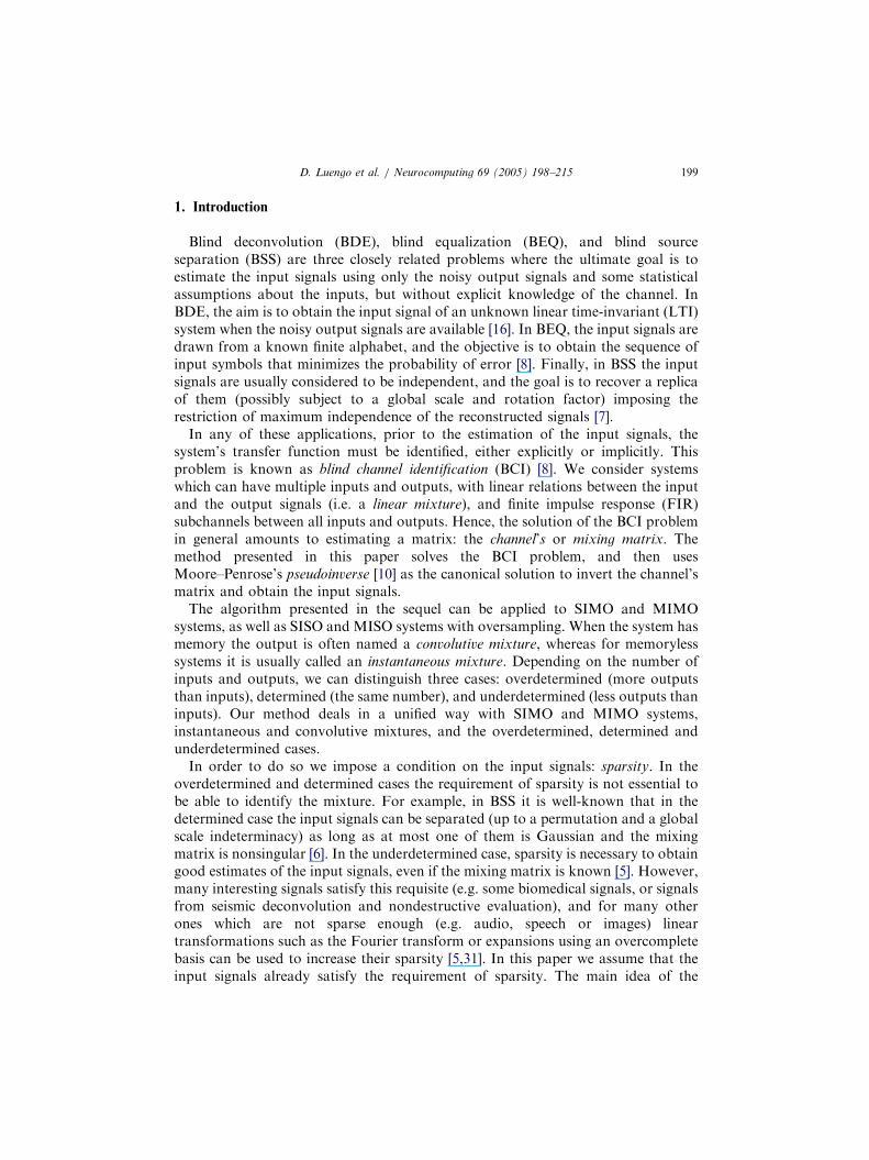
Thus, in the absence of noise the output vector is aligned with the kth colum(i.e. the direction of ~yðnÞ is given by the kth basis vector, ~hk). When the outputare corrupted by noise, the direction of ~yðnÞ will be spread around the true digiven by ~hk. In moderate/high signal to noise ratio (SNR) situations, this resuclustering of the output vectors around the basis vectors, which can be exploidentify them [5,9]. Fig. 1 shows a typical scatter plot of the componentsoutput vector, which displays the clustering characteristic of sparse input sThe data, generated synthetically using the BG model and a mixing matrix gi

~H ¼0:3500 �0:3696 0:8600 0:1732 �0:1854

0:6062 0:1531 �0:5000 0:1000 �0:5706

� �closely resemble the time series typical of applications such as seismic deconvo(see Fig. 5 for a time-domain representation using a different ~H).

3.2. Model of the output signals

In order to develop the different stages of the algorithm we require a stamodel of the output signals. Since the algorithm is based on the clustering

Fig. 1. Scatter plot of the output signals mixed with (11) using the BG model for the sources with s2s ¼ 1,

p ¼ 0:75, N ¼ 10000, and SNR ¼ 30 dB.

outputs around the basis vectors when there is only one nonzero input, we just neednd fored foractive,sion ofof the

ð12Þ

outputN andvector

(13)

ith ~hk),of the

ð14Þ

the kth

ARTICLE IN PRESS

D. Luengo et al. / Neurocomputing 69 (2005) 198–215204

a model for this case. Considering an equal variance for all the sources, s2s , aall the samples of the noise vector, s2w, the PDF of ~yðnÞ can be easily obtainm ¼ 2. In the absence of noise, and assuming that only the kth input signal isthe PDF of each of the components of the output vector is simply a scaled verthe PDF of sk. Since both outputs follow a deterministic relation, the PDFoutput vector is

f ~X ð~xðnÞÞ ¼1

jhkð1Þjf Sk

x1ðnÞ

hkð1Þ

� d x2ðnÞ �

hkð2Þ

hkð1Þx1ðnÞ

� ¼

1

jhkð2Þjf Sk

x2ðnÞ

hkð2Þ

� d x1ðnÞ �

hkð1Þ

hkð2Þx2ðnÞ

� .

Since the noise is white and independent of the sources, the PDF of the noisyvector is simply (12) convolved with the PDF of the noise. Considering AWGthe BG model, we obtain a zero-mean bivariate Gaussian PDF for the outputcharacterized by an autocorrelation matrix [15]

~Ry ¼ s2s~hk~hT

k þ s2w~I .

If we have Nk samples for which this happens (i.e. for which ~xðnÞ is aligned wthe global PDF is their product. Hence, the log-likelihood function in termsmagnitude and angle of the kth column is [15]

ln f ~Y ð~yÞ ¼ �Nk

2lnðr2ks

2s þ s2wÞ

þs2s r2k

2s2wðr2ks

2s þ s2wÞ

Xnk

ðy1ðnkÞ cos yk þ y2ðnkÞ sin ykÞ2,

where the constant terms that do not depend on the angle or magnitude ofbasis vector have been omitted, and nk ¼ fn : arctanðx2ðnÞ=x1ðnÞÞ ¼ ykg.

4. Description of the algorithm

ing themixingture tosystemand ahe five

beddedcriteria

In this section we describe in detail the five stages of the algorithm: detectnumber of input signals, estimating the direction of each basis vector of thematrix, estimating their magnitudes, ordering them, and inverting the mixobtain the input signals. As discussed previously, in the case of a memorylessthe third and fourth steps are not required, since a global scale factorpermutation in the input signals are admissible. If the system has memory tsteps are essential.

4.1. Detection of the number of input signals

The standard way of detecting the number of narrowband input signals emin a set of observations contaminated by noise is using information theoretic

such as Akaike’s information criterion (AIC) or Schwartz and Rissanen’s minimumsignalslus anproachequiresto thed haverequire

m ¼ 2.12], ansed asquired

ARTICLE IN PRESS

D. Luengo et al. / Neurocomputing 69 (2005) 198–215 205

description length (MDL) principle [30]. Both of them select the number ofwhich minimizes a cost function composed of the log-likelihood function padditional term which penalizes the complexity of the model. However, the appresented in [30], based on the eigenvalues of the sample covariance matrix, rmore outputs than inputs, and consequently cannot be applied directlyunderdetermined case. Several modifications and improvements of this methobeen presented, and some other algorithms are also available, but all of themlom.Nevertheless, in [15] the algorithm of [30] has been extended to the case

Noting the similarities between a power spectral density (PSD) and a PDF [autocorrelation matrix can be constructed from the PDF of the angle, and uthe sample covariance matrix for the algorithm presented in [30]. The steps reto detect the number of sources are the following:

(1) Obtain an N 1 vector of angles from the output signals:

(15)

in annsform

eyðnÞ ¼ arctany2ðnÞ

y1ðnÞ,

where �poeyðnÞpp, and n ¼ 0; . . . ;N � 1.(2) Noting the similarity between a PDF and a PSD, we may obta

‘‘autocorrelation function’’ (ACF) for the angles as the inverse Fourier tra

(16)

(17)

ði; jÞth

(IFT) of the estimated PDF of y [12]. Using a train of impulses at the anthe output signals as the estimated PDF,

pYðyÞ ¼1

N

XN�1

n¼0

dðy� eyðnÞÞand taking its IFT, the ACF of the angles becomes

RY½k ¼1

2pN

XN�1

n¼0

expðjkeyðnÞÞ,i.e. samples of the characteristic function for k ¼ 0; . . . ;N � 1.

(3) Construct the global autocorrelation matrix (ACM) using (17), so that itselement is given by ~RY ¼ RY½i � j ¼ R

½j � i.

eoretic

(4) Now, for increasing model orders (i ¼ 1; . . . ;M), apply an information thcriterion (ITC) using the first i columns and rows of the ACM:

(18)

ameterof thent thethe ithwhichse, the

ITCðiÞ ¼ � ln f ~Y ð~yjfðiÞÞ þ CðNÞvðiÞ,

where the first term is the log-likelihood function conditioned by the parset of the ith hypothesis, f

ðiÞ, and the second term penalizes the complexity

model. It is composed of CðNÞ, which is a function that takes into accousize of the data set, and vðiÞ, which is the number of free parameters ofhypothesis. The two most commonly used ITCs are the AIC [2], forCðNÞ ¼ 1, and the MDL [19,20], for which CðNÞ ¼ 1

2lnN. In this ca

number of free parameters for both of them is vðiÞ ¼ ið2M � iÞ [30]. Since theuse theM [30]:

(19)

es (19).

ARTICLE IN PRESS

15 20 25 30 35 400

0.1

0.2

0.3

0.4

0.5

0.6

0.7

0.8

0.9

1

SNR (dB)

Det

ectio

n P

roba

bilit

y

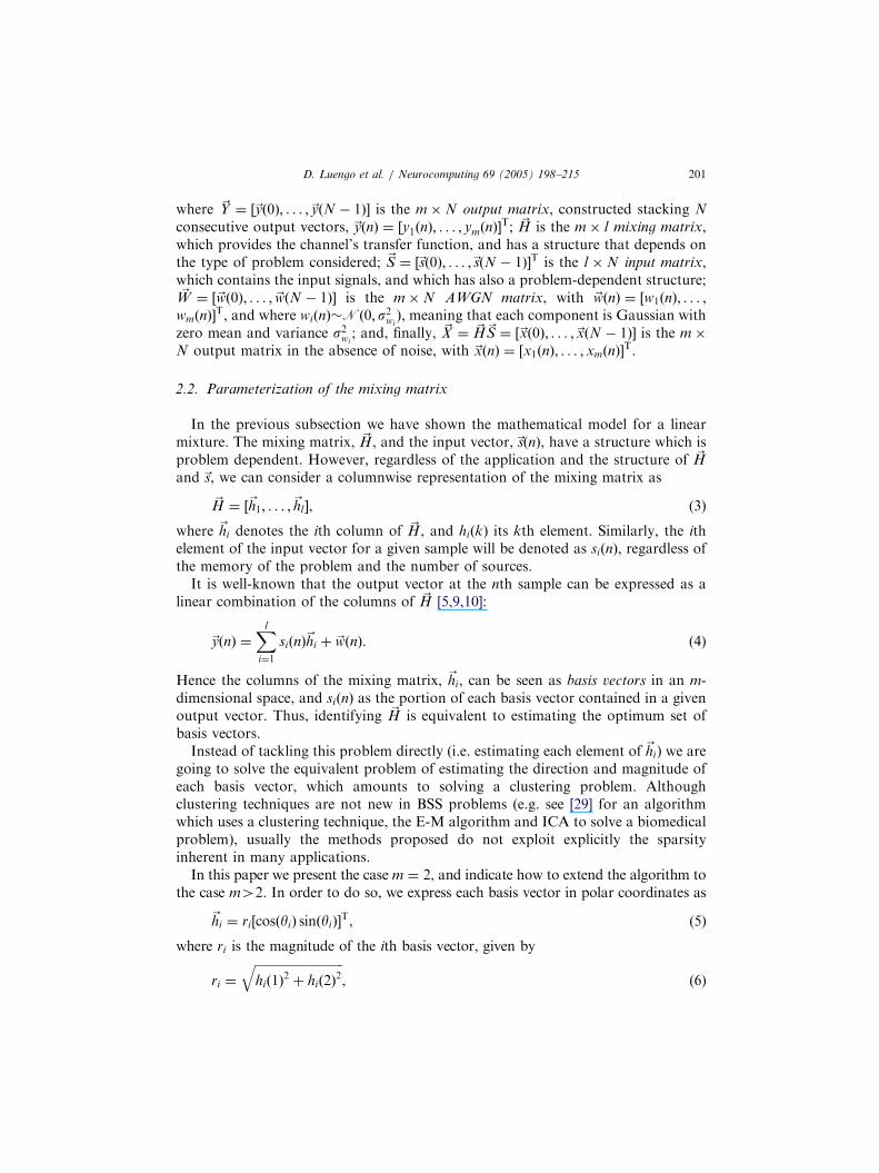
Inst. (p = 0.6)Inst. (p = 0.75)Conv. (p = 0.6)Conv. (p = 0.75)Conv. (p = 0.9)

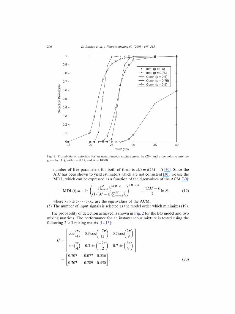
Fig. 2. Probability of detection for an instantaneous mixture given by (20), and a convolutive mixture

given by (11), with p ¼ 0:75, and N ¼ 10000.

D. Luengo et al. / Neurocomputing 69 (2005) 198–215206

AIC has been shown to yield estimators which are not consistent [30], weMDL, which can be expressed as a function of the eigenvalues of the AC

MDLðiÞ ¼ � ln

QMj¼iþ1l

1=ðM�iÞj

ð1=ðM � iÞÞPM

j¼iþ1lj

!ðM�iÞN

þið2M � iÞ

2lnN,

where l14l24 � � �4lm are the eigenvalues of the ACM.(5) The number of input signals is selected as the model order which minimiz

nd two

ð20Þ

mixing matrices. The performance for an instantaneous mixture is tested usfollowing 2 3 mixing matrix [14,15]:

~H ¼

cosp4

�0:3 cos

�7p12

� 0:7 cos

2p9

� sin

p4

�0:3 sin

�7p12

� 0:7 sin

2p9

� 266664

377775¼

0:707 �0:077 0:536

0:707 �0:289 0:450

" #.

The performance for a convolutive mixture is tested using the 2 5 mixing matrix

m ¼ 2,proaches canderate/native,s usednsiderthan aimatedolutionmatingnce ofsistent

rs (i.e.nmentsignalach ise veryn alsomation-based

D, anda PSDniquesSPRITwever,highuse acardedder theed bin.

angles

ARTICLE IN PRESS

D. Luengo et al. / Neurocomputing 69 (2005) 198–215 207

given by (11).Although this method provides good results for moderate/high SNRs and

it cannot be directly extended to the case m42. In these cases, a simple apbased on setting a threshold in the multidimensional PDF of the anglbe considered. This approach shows a satisfactory performance for mohigh SNRs, but requires the setting of a subjective threshold. A better alterif a clustering method such as the competitive one presented in [13] ifor the next step, is to start with a high number of basis vectors and cosome merging strategy (e.g. two vectors merge when they differ in lessgiven angle). The final number of basis vectors equals the number of estinput signals. This method presents the advantage of providing a joint sto the first two problems: detecting the number of signals and estithe directions of the basis vectors. However, the issue of convergeany clustering algorithm should be carefully considered to ensure consolutions.

4.2. Estimation of the direction of the basis vectors

There are several ways to estimate the directions of the basis vectothe columns of the mixing matrix), but they are all based on the aligbetween the output vectors and the basis vectors when only one inputis different from zero. In [5] a potential function based clustering approused. In [9] an approach based on Parzen windowing is shown to providgood results. The competitive clustering approach presented in [13] cabe used. However, in this paper we consider two alternatives: the estifrom the PSD considered in the previous section, and an histogramestimator.In the previous section we noted the close relation between a PDF and a PS

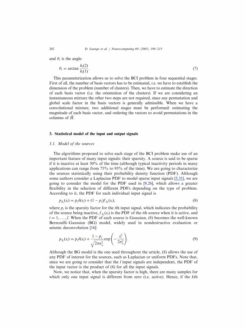
constructed an ACF (17). Taking the Fourier transform of (17) we obtainfunction, and can apply any of the rich variety of spectral estimation techavailable [22]. This approach has already been considered in [28], where the Emethod was used to estimate the peaks corresponding to each basis vector. Hoalthough this method provides very good results, it also requires acomputational cost. Thus, as a cost-efficient alternative, we are going tohistogram-based estimator. This approach was considered in [9] and disbecause of its poor results. Nevertheless, it can be greatly improved if we consiML estimator of the angles inside each bin, instead of the center of the selectThe method proceeds as follows:

(1) Construct a histogram of angles in the range ½0; p from the set of

oid the

estimated previously for each output signal, eyðnÞ. An example of aestimated PDF for the mixture given by (11) is shown in Fig. 3.

(2) Select the m highest peaks of the histogram, establishing a strategy to avdetection of false peaks due to noise.

(3) Apply the ML estimator for the angles inside each of the selected bins. If wetor for

ARTICLE IN PRESS

−1.5 −1 −0.5 0 0.5 1 1.50

0.002

0.004

0.006

0.008

0.01

0.012

0.014

0.016

0.018

θ

p Θ (θ

)

Fig. 3. Example of the estimated PDF (histogram) of the angle for a convolutive mixture given by (11)

with p ¼ 0:9, and SNR ¼ 30dB.

D. Luengo et al. / Neurocomputing 69 (2005) 198–215208

(21)

the Nk

consider a BG model, it can be easily seen from (14) that the ML estimathe angle of the kth basis vector is [15]

yk ¼1

2arctan

2~yT1~y2~yT1~y1 �~yT2~y2

!,

where ~y1 and ~y2 are the vectors with the first and second components ofoutput signals whose angle falls inside the kth selected bin.

Note that, when the exact PDF of the input signals is unknown or the MLng thendent.fficultygramsowingm ¼ 3o be aequateains an

estimator cannot be obtained, we can estimate the angles simply averagiestimates which fall inside each selected bin, making this stage PDF-indepeThis approach provides good results for m ¼ 2, but presents an increasing diand computational cost as m increases (searches in ðm � 1Þ-dimensional histoare required). The same happens for the potential function and Parzen windapproaches, and the approach based on the PSD (although an estimator forhas been proposed in [27]). The only viable alternative for high m seems tclustering approach such as the one presented in [13]. However, the adinitialization of the basis vectors for this algorithm is a delicate task and remopen problem.

4.3. Estimation of the amplitude of the basis vectors

tationsolved,ignals.of theamplesapplyd from

(22)

can beDF ofthosete that

(23)

utputse used

(24)

mporalon thepipq)mns ofs muste basiswith li

whichorder,on theSNR

nd thee BCIaneousor the

ARTICLE IN PRESS

D. Luengo et al. / Neurocomputing 69 (2005) 198–215 209

So far we have identified the mixing matrix up to a scale and a permuindeterminacy. In the case of an instantaneous mixture the BCI problem isand the only remaining step is inverting the mixture to obtain the input sHowever, for convolutive mixtures we need to estimate the relative amplitudescolumns and their order. From the previous section we have a set of sapproximately aligned with each of the l basis vectors. Hence, we can easilythe ML estimator of their magnitudes for each bin, which is readily obtaine(14) [15]:

rk ¼

ffiffiffiffiffiffiffiffiffiffiffiffiffiffiffiffiffiffiffiffiffiffiffiffiffiffiffiffiffiffiffiffiffiffiffiffiffiffiffiffiffiffiffiffiffiffiffiffiffiffiffiffiffiffiffiffiffiffiffiffiffiffiffiffiffiffiffiffiffiffiffiffiffiffiffiffiffiffiffiffiffiffiffiffiffiffiffiffiffiffiffiffiffiffiffiffiffiffiffiffiffiffiffiffiffið~y1 cos yk þ~y2 sin ykÞ

Tð~y1 cos yk þ~y2 sin ykÞ � Nks2wNks2s

s,

where ~y1 and ~y2 are the vectors obtained in the previous stage. This approacheasily extended for m42. Its main restriction is that it is dependent on the Pthe input signals, which may not be precisely known for some applications. Incases, when the noise is zero mean and independent of the input signals, we no

Ef~yðnkÞT~yðnkÞg ¼ s2s r2k þ s2w,

where Ef�g denotes the mathematical expectation, taken over the set of oaligned with the kth basis vector. Hence, in these cases the sample mean can bto estimate the magnitude of each column of ~H:

rk ¼

ffiffiffiffiffiffiffiffiffiffiffiffiffiffiffiffiffiffiffiffiffiffiffiffiffiffiffiffiffiffiffiffiffiffiffiffiffiffiffiffiffiffiffiffiffiffiffiffiffiPnk~yðnkÞ

T~yðnkÞ � Nks2wNks2s

s.

4.4. Ordering the basis vectors

The permutation indeterminacy can be removed by exploiting the tecorrelation between consecutive input vectors. The ordering method is basedfact that, in the absence of noise, a nonzero sample of the ith source (1surrounded by li � 1 zeros is sequentially aligned with the li consecutive coluthe mixing matrix related to its impulse response. Obviously, the other sourcealso be inactive during those samples. Hence, we can estimate the order of thvectors considering the set of output samples which are sequentially aligneddifferent basis vectors, and setting the most likely column order as the oneappears most often. In a certain sense this is the ML estimator of the columnsince we are estimating the most likely order of the basis vectors basedempirical PDF of their order, and works very well under moderate/highconditions.At this point the BCI problem has been solved, both for the instantaneous a

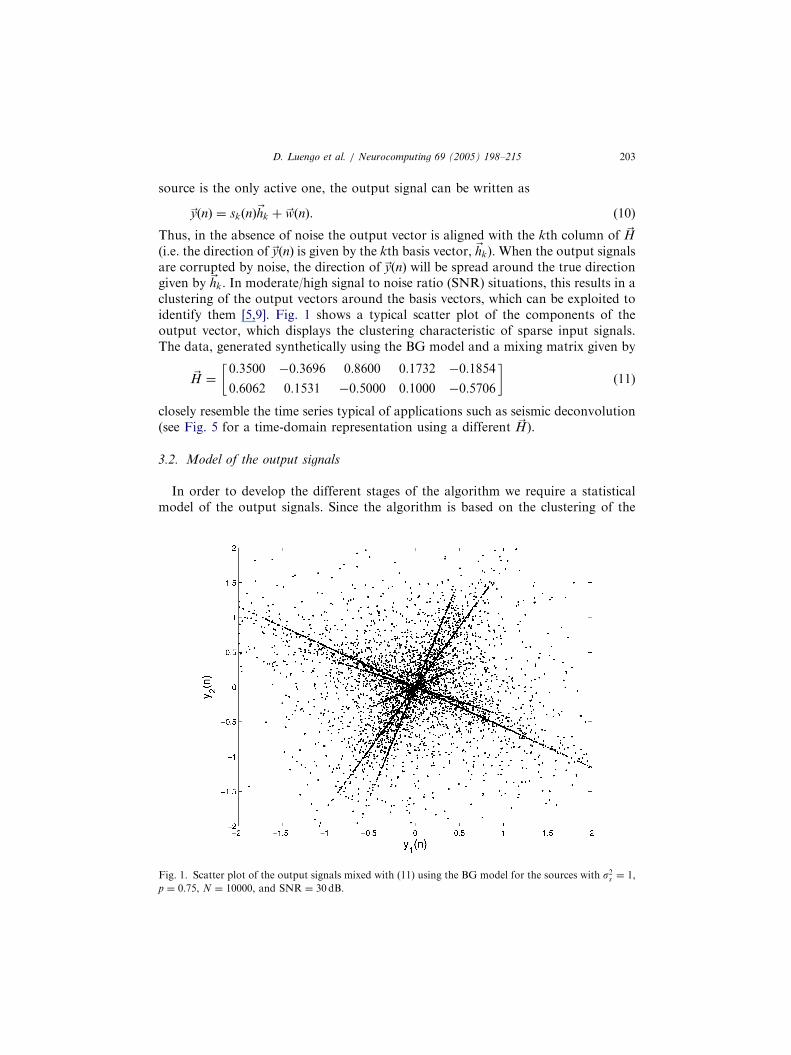
convolutive mixtures. As an example of the performance of the wholalgorithm, Fig. 4 shows the MSE obtained for the outputs for the instantmixture using (20) and the convolutive mixture using (11). The results f

convolutive mixture are 2–5 dB worse than for the instantaneous mixture due to theby the

by theolutionIn them [10],s beenple, ins beene suchd withhereasof thee closef noise

ARTICLE IN PRESS

10 15 20 25 30 35 4010

15

20

25

30

35

SNR (dB)

−10

log 1

0 (M

SE

)

N = 1000N = 2000N = 5000N = 10000

Fig. 4. Normalized MSE (dB) as a function of the SNR for p ¼ 0:8 and ~H given by (20) for the

instantaneous mixture (dashed line) and (11) for the convolutive mixture (continuous line).

D. Luengo et al. / Neurocomputing 69 (2005) 198–215210

increased number of sources, and the additional variance introducedmagnitude estimation step.

4.5. Inverting the mixture

In the determined case the input signals are completely characterizedmixing matrix. In the overdetermined case, the pseudoinverse provides the swith minimun L2 norm of the error, and hence it is commonly used.underdetermined case, the pseudoinverse is the solution with minimum L2 norand thus can be considered the canonical inversion strategy. However, it hashown in [26] that much better inversion strategies can be developed. For exam[26] a Bayesian inversion strategy, which has a high computational cost, hadeveloped, altogether with several heuristic criteria. In this paper we use onsimple heuristic criterion for the inversion: the output signals which are alignesome basis vector are inverted using only the corresponding column of ~H, wthe rest of the outputs are inverted using the pseudoinverse. An exampleinversion of the mixture is shown in Fig. 5 for the instantaneous case, where thresemblance of both signals, in spite of a scale factor and the appearance opeaks, can be appreciated.

5. Applications

on theuctures

signalsvectorþ ðj �

tructedoposed-ordernsionslts, butuld beis case

ARTICLE IN PRESS

0 100 200 300 400 500 600 700 800 900 1000

-2

-1

0

1

2

n

Orig

inal

sig

nal

0 100 200 300 400 500 600 700 800 900 1000

-2

-1

0

1

2

n

Rec

over

ed s

igna

l

Fig. 5. Example of an original input signal and the recovered signal for an instantaneous mixture given by

(20) with p ¼ 0:9 and SNR ¼ 30 dB.

D. Luengo et al. / Neurocomputing 69 (2005) 198–215 211

In Section 2.1 it was pointed out that the structure of ~H and~sðnÞ dependedproblem at hand. In this section we describe briefly the different possible strand some associated applications.

5.1. SISO systems with oversampling

In this case there is a single source, sðnÞ, and channel, hðnÞ. Multiple outputare obtained using an oversampling ratio m. Now the elements of the inputare siðnÞ ¼ sðn � iÞ, and the elements of the channel’s matrix are hij ¼ hði � 11ÞmÞ for i; j ¼ 1; . . . ;N.This approach is very common in BEQ, where a SIMO system can be cons

from a SISO problem by oversampling [8]. Using this technique Tong et al. pran algorithm based on subspace methods for identifying ~H using only secondstatistics of the output signals [24,25]. Since then, there have been several exteof this idea (see for example [1,17,23]). These methods provide very good resuhave a high computational cost. The algorithm described in this article coapplied to obtain a low cost solution of the problem. The main challenge in this finding a domain where the input signals are sparse enough.

5.2. SIMO systems with convolutive mixtures

ðn � iÞ,tes the

lutionsponses. The(ML)ay be

e oftenithout

ixture.linearix, hij ,

use itss. Thebasedeoreticng andoposednd canBCI in

h q41olutiveusuallyable toe othernough.

ARTICLE IN PRESS

D. Luengo et al. / Neurocomputing 69 (2005) 198–215212

In this case, the ith element of the input vector at time n is again siðnÞ ¼ s

and the elements of the mixing matrix are hij ¼ hiðn � j � 1Þ, where hið�Þ denosubchannel from the input to the ith observation.This situation is typical in many BDE problems, such as seismic deconvo

[16] and nondestructive evaluation [21], where the output of the system in reto an input signal is measured using several sensors placed at different locationstandard approach to this problem is to perform maximum likelihooddeconvolution [16], but due to its high computational cost simpler methods mpreferred in some cases. Besides, in these applications the input signals arsparse enough to apply the techniques of the article in the time domain, wtransforming them into any other domain.

5.3. MIMO systems with instantaneous mixtures

The simplest MIMO systems are those in which we have an instantaneous mIn this case, the nth sample of the observation vector is simply a weightedcombination of the input signals. Thus, each element of the mixing matrrepresents the contribution of the jth source to the ith observation.This is the most widely used model in blind source separation (BSS), beca

simplicity allows the obtention of good solutions under certain assumptiondetermined case has been widely studied, and excellent solutions are availableon statistical principles, independent component analysis, and information thcriteria (see for example [4,6,11]). The underdetermined case is more challengihas received little attention until recently, when several methods have been pr[5,9,31]. The algorithm presented in this paper follows a similar approach, abe considered an extension of the methods presented separately for BSS and[9,14,15].

5.4. MIMO systems with convolutive mixtures

The last case is a combination of the two previous problems: a system witsources, and memory. This problem appears typically in BSS with convmixtures [7], and in BEQ of MIMO communication systems [8,18], and issolved in the frequency domain [3]. The algorithm presented in this article issolve the MIMO problem with convolutive mixtures in the same way as ththree problems, in the time domain, as long as the input signals are sparse e

6. Conclusions

solvingblind

oposed

In this paper we have presented a computationally efficient algorithm forinverse problems when the input signals are sparse, which can be applied todeconvolution, blind equalization, and blind source separation. The pr

method takes advantage of the sparsity of the input signals and a parameterizationlve thematinge basishe BGm42to anourcesy using

ARTICLE IN PRESS

D. Luengo et al. / Neurocomputing 69 (2005) 198–215 213

of the columns of the mixing matrix (basis vectors) in polar coordinates to soproblem in five sequential stages: detecting the number of input signals, estithe directions of the basis vectors, estimating their amplitudes, ordering thvectors, and inverting the mixture. Explicit formulas have been provided for tmodel and m ¼ 2, and considerations for the extension to different PDFs andhave been done. Future research lines include the extension of the methodarbitrary number of output signals, to different PDFs of the sources or even swith unknown PDFs, and for nonlinear and post-nonlinear mixtures, possiblspectral clustering techniques.

References

er blind

l AC-19

ation of

. Speech

nd blind

ntations,

–2025.

02.

g matrix

rence on

A, 2001,

ty Press,

, Neural

tt. 5 (12)

s testing:

channel

1.

f sparse

national

279–288.

tification

s—a key

[1] K. Abed-Meraim, E. Moulines, P. Loubaton, Prediction error methods for second-ord

identification, IEEE Trans. Signal Process. 45 (3) (1997) 694–705.

[2] H. Akaike, A new look at the statistical model identification, IEEE Trans. Automat. Contro

(1974) 716–723.

[3] S. Araki, R. Mukai, S. Makino, T. Nishikawa, H. Saruwatari, The fundamental limit

frequency domain blind source separation for convolutive mixtures of speech, IEEE Trans

Audio Process. 11 (2) (2003) 109–116.

[4] A.J. Bell, T.J. Sejnowski, An information–maximization approach to blind separation a

deconvolution, Neural Comput. 7 (1995) 1129–1159.

[5] P. Bofill, M. Zibulevsky, Underdetermined blind source separation using sparse represe

Signal Process. 81 (11) (2001) 2353–2362.

[6] J.F. Cardoso, Blind signal separation: statistical principles, Proc. IEEE 86 (10) (1998) 2009

[7] A. Cichocki, S. Amari, Adaptive Blind Signal and Image Processing, Wiley, New York, 20

[8] Z. Ding, Y.G. Li, Blind Equalization and Identification, Marcel Dekker, New York, 2001.

[9] D. Erdogmus, L. Vielva, J.C. Prıncipe, Nonparametric estimation and tracking of the mixin

for underdetermined blind source separation, in: Proceedings of the International Confe

Independent Component Analysis and Blind Signal Separation (ICA), San Diego, CA, US

pp. 189–193.

[10] G.H. Golub, C.F. Van Loan, Matrix Computations, 3rd ed., The John Hopkins Universi

Baltimore, MD, USA, 1996.

[11] A. Hyvarinen, E. Oja, Independent component analysis: algorithms and applications

Networks 13 (4–5) (2000) 411–430.

[12] S.M. Kay, Model-based probability density function estimation, IEEE Signal Process. Le

(1998) 318–320.

[13] D. Luengo, C. Pantaleon, I. Santamarıa, L. Vielva, J. Ibanez, Multiple composite hypothesi

a competitive approach, J. VLSI Signal Process. 37 (2004) 319–331.

[14] D. Luengo, I. Santamarıa, J. Ibanez, L. Vielva, C. Pantaleon, A fast blind SIMO

identification algorithm for sparse sources, IEEE Signal Process. Lett. 10 (5) (2003) 148–15

[15] D. Luengo, I. Santamarıa, L. Vielva, C. Pantaleon, Underdetermined blind separation o

sources with instantaneous and convolutive mixtures, in: Proceedings of the XIII IEEE Inter

Workshop on Neural Networks for Signal Processing (NNSP), Toulouse, France, 2003, pp.

[16] J.M. Mendel, Maximum Likelihood Deconvolution, Springer, Berlin, 1990.

[17] E. Moulines, P. Duhamel, J.F. Cardoso, S. Mayrargue, Subspace methods for the blind iden

of multichannel FIR filters, IEEE Trans. Signal Process. 43 (2) (1995) 516–525.

[18] A.J. Paulraj, D.A. Gore, R.U. Nabar, H. Bolcskei, An overview of MIMO communication

to gigabit wireless, Proc. IEEE 92 (2) (2004) 198–218.

[19] J. Rissanen, Modeling by shortest data description, Automatica 14 (1978) 465–471.

[20] G. Schwartz, Estimating the dimension of a model, Ann. Statist. 6 (1978) 461–464.

structive

J, 1997.

tatistics:

ultipath

rs, 1991,

tistics: a

babilistic

ependent

675–679.

d BSS in

rence on

n, 2003,

n of the

iques, in:

560.

, K. Li,

II IEEE

ce, 2003,

Acoust.

a signal

ived the

nication

nd 1998,

at the

antabria,

boratory

os III at

research

ing and

tion.

ARTICLE IN PRESS

D. Luengo et al. / Neurocomputing 69 (2005) 198–215214

[21] S.K. Sin, C.H. Sen, A comparison of deconvolution techniques for the ultrasonic nonde

evaluation of materials, IEEE Trans. Image Process. 1 (1) (1992) 3–10.

[22] P. Stoica, R.L. Moses, Introduction to Spectral Analysis, Prentice-Hall, Englewood Cliffs, N

[23] L. Tong, G. Xu, B. Hassibi, T. Kailath, Blind channel identification based on second-order s

a frequency domain approach, IEEE Trans. Inform. Theory 41 (1) (1995) 329–334.

[24] L. Tong, G. Xu, T. Kailath, A new approach to blind identification and equalization of m

channels, in: Proceedings of the Asilomar Conference on Signals, Systems, and Compute

pp. 856–860.

[25] L. Tong, G. Xu, T. Kailath, Blind identification and equalization based on second-order sta

time domain approach, IEEE Trans. Inform. Theory 40 (2) (1994) 340–349.

[26] L. Vielva, D. Erdogmus, J.C. Prıncipe, Underdetermined blind source separation using a pro

source sparsity model, in: Proceedings of the Second International Conference on Ind

Component Analysis and Blind Signal Separation (ICA), San Diego, CA, USA, 2001, pp.

[27] L. Vielva, Y. Pereiro, D. Erdogmus, J.C. Prıncipe, Inversion techniques for underdetermine

an arbitrary number of dimensions, in: Proceedings of the Fourth International Confe

Independent Component Analysis and Blind Signal Separation (ICA), Nara, Japa

pp. 131–136.

[28] L. Vielva, I. Santamarıa, C. Pantaleon, J. Ibanez, D. Erdogmus, J.C. Prıncipe, Estimatio

mixing matrix for underdetermined blind source separation using spectral estimation techn

Proceedings of the XI European Signal Processing Conference (EUSIPCO), 2002, pp. 557–

[29] Y. Wang, J. Xuan, R. Srikanchana, J. Zhang, Z. Szabo, Z. Bhujwalla, P. Choyke

Computed simultaneous imaging of multiple biomarkers, in: Proceedings of the XI

International Workshop on Neural Networks for Signal Processing (NNSP), Toulouse, Fran

pp. 269–278.

[30] M. Wax, T. Kailath, Detection of signals by information theoretic criteria, IEEE Trans.

Speech Signal Process. ASSP-33 (2) (1985) 387–392.

[31] M. Zibulevsky, B.A. Pearlmutter, Blind source separation by sparse decomposition in

dictionary, Neural Comput. 13 (2001) 863–882.

David Luengo was born in Santander, Spain, in 1974. He rece

Radiocommunication Bachelor Engineer degree and the Telecommu

Engineer Degree from the University of Cantabria, Spain, in 1994 a

respectively. From 1998 to 2003 he was a Research Associate

Departamento de Ingenierıa de Comunicaciones, Universidad de C

Spain. In 2002, he spent a visiting period at the Coordinated Science La

(CSL), University of Illinois. In 2003 he joined the Universidad Carl

Madrid, where he is currently an Assistant Professor. His current

interests include applications of chaos theory to signal process

communications, machine learning algorithms, and blind source separa

and the

d, Spain,

genierıa

ently an

at the

Florida.

journals

include

gorithms

Ignacio Santamarıa received the Telecommunication Engineer Degree

Ph.D. in electrical engineering from the Polytechnic University of Madri

in 1991 and 1995, respectively. In 1992 he joined the Departamento de In

de Comunicaciones, Universidad de Cantabria, Spain, where he is curr

Associate Professor. He held visiting positions in 2000 and 2004

Computational NeuroEngineering Laboratory (CNEL), University of

He has authored and coauthored more than 70 publications in refereed

and international conference papers. His current research interests

nonlinear modelling techniques, adaptive systems, machine learning al

and their application to digital communication systems.

Luis Vielva was born in Santander, Spain, in 1966. He received his Licenciado

antabria,

ento de

ere he is

d at the

Florida.

national

paration

ARTICLE IN PRESS

D. Luengo et al. / Neurocomputing 69 (2005) 198–215 215

degree in Physics and his Ph.D. in Physics from the University of C

Spain in 1989 and 1997, respectively. In 1989 he joined the Departam

Ingenierıa de Comunicaciones, Universidad de Cantabria, Spain, wh

currently an Associate Professor. In 2001, he spent a visiting perio

Computational NeuroEngineering Laboratory (CNEL), University of

Dr. Vielva has more than 50 publications in refereed journals and inter

conference papers. His current research interests include blind source se

and bioinformatics.