A general predictive model for estimating monthly ecosystem evapotranspiration

ECOHYDROLOGYEcohydrol. 4, 245–255 (2011)Published online 29 December 2010 in Wiley Online Library(wileyonlinelibrary.com) DOI: 10.1002/eco.194

A general predictive model for estimating monthly ecosystemevapotranspiration

Ge Sun,1* Karrin Alstad,2 Jiquan Chen,2 Shiping Chen,3 Chelcy R. Ford,4 Guanghui Lin,3

Chenfeng Liu,5 Nan Lu,2 Steven G. McNulty,1 Haixia Miao,3 Asko Noormets,6

James M. Vose,4 Burkhard Wilske,2 Melanie Zeppel,7 Yan Zhang5

and Zhiqiang Zhang5

1 Eastern Forest Environmental Threat Assessment Center, USDA Forest Service, Raleigh, NC, USA2 Department of Environmental Sciences, University of Toledo, Toledo, OH, USA

3 Institute of Botany, Chinese Academy of Sciences, Beijing, China4 Coweeta Hydrologic Laboratory, USDA Forest Service, Otto, NC, USA

5 College of Soil and Water Conservation, Beijing Forestry University, Beijing, China6 Department of Forestry and Environmental Resources, North Carolina State University, Raleigh, NC, USA

7 Department of Biology, Macquarie University, Sydney, Australia

ABSTRACT

Accurately quantifying evapotranspiration (ET) is essential for modelling regional-scale ecosystem water balances. This studyassembled an ET data set estimated from eddy flux and sapflow measurements for 13 ecosystems across a large climatic andmanagement gradient from the United States, China, and Australia. Our objectives were to determine the relationships amongmonthly measured actual ET (ET), calculated FAO-56 grass reference ET (ETo), measured precipitation (P), and leaf areaindex (LAI)—one associated key parameter of ecosystem structure. Results showed that the growing season ET from wetforests was generally higher than ETo while those from grasslands or woodlands in the arid and semi-arid regions were lowerthan ETo. Second, growing season ET was found to be converged to within š10% of P for most of the ecosystems examined.Therefore, our study suggested that soil water storage in the nongrowing season was important in influencing ET and wateryield during the growing season. Lastly, monthly LAI, P, and ETo together explained about 85% of the variability of monthlyET. We concluded that the three variables LAI, P, and ETo, which were increasingly available from remote sensing productsand weather station networks, could be used for estimating monthly regional ET dynamics with a reasonable accuracy. Suchan empirical model has the potential to project the effects of climate and land management on water resources and carbonsequestration when integrated with ecosystem models. Copyright 2010 John Wiley & Sons, Ltd.

KEY WORDS climate change; ET; eddy flux; modelling; sapflow; water balance

Received 27 January 2010; Accepted 4 December 2010

INTRODUCTION

Evapotranspiration (ET) accounts for over half of thetotal water loss from most terrestrial vegetated ecosys-tems (Zhang et al., 2001; Lu et al., 2003). For example,in water-limited semi-arid and arid regions, ET can com-prise an even greater percentage of the total water loss(Wang et al., 2010) and can equal precipitation. Changesin land use/land cover and climate can also directlyimpact water supply and demand and the regional hydro-logical cycle (DeWalle et al., 2000; Jackson et al., 2001;Foley et al., 2005; Liu et al., 2008; Sun et al., 2008a) byaltering the ET processes. Although ET is a key vari-able that links hydrological and biological processes inmost ecosystem models (Hanson et al., 2004), ET is oneof the most difficult water budget components to quan-tify (Allen, 2008; Shuttleworth, 2008). Worldwide hightemporal scale ET measurements based on soil water

* Correspondence to: Ge Sun, Eastern Forest Environmental ThreatAssessment Center, USDA Forest Service, Raleigh, NC, USA.E-mail: ge [email protected]

balance, sapflow, and eddy covariance methods offerednew insights in ecohydrological sciences and helped toadvance our understanding of the ET processes. Sev-eral techniques for quantifying ET exist; for example,the watershed water balance method of precipitation (P)inputs minus streamflow outputs (Q), or ET D P � Q, istypically limited to long-term average, when the changein water storage component is negligible (Wilson et al.,2001; Ford et al., 2007). At the other temporal extreme,sapflow- and eddy covariance-based ET estimates agreewell with other techniques for uniform stands with largefootprints (i.e. continuous coverage), but are less reliablein complex stands and small or nonuniform footprints(i.e. canopy gaps) (Wullschleger et al., 1998; Wilsonet al., 2001; Ewers et al., 2002; Law et al., 2002; Arainet al., 2003; Paw U, 2006; Ford et al., 2007; Sun et al.,2008a, 2009, 2010; Barker et al., 2009). Eddy covari-ance and sapflow methods have gained popularity forsimultaneously measuring both water and carbon fluxesbecause of their ability to resolve fluxes on a short time-step, offering high temporal resolution. This is largely

Copyright 2010 John Wiley & Sons, Ltd.

246 G. SUN et al.

due to performance improvements and reduced costs offast-response monitoring equipment in recent years. Ageneral predictive model of ET at a monthly scale couldhelp land managers to maximize the ecosystem servicesbecause ET is highly coupled with carbon gain (Lawet al., 2002; Jackson et al., 2005; Noormets et al., 2006)and other ecosystem services such as biodiversity (Currie,1991).

Biophysical modelling has been the most popularapproach for estimating the regional ET using mass-and energy balance theories and empirical relationshipsamong potential ET, precipitation or soil moisture sta-tus, and/or land cover type (Zhang et al., 2001; Lu et al.,2003; Amatya and Trettin, 2007; Zhou et al., 2008).Energy and water balances of terrestrial ecosystems aretightly coupled through the ET processes at multiplescales. The long-term ET for a large area is mainlycontrolled by water and energy availability and by landsurface characteristics to a minor extent (Milly, 1994;Zhang et al., 2001, 2004). Although a comparison ofBudyko-type models that describe such energy–waterrelationships is found in Zhang et al. (2004), quantifyingET of vegetated surfaces at a fine spatial and temporalscale (e.g. watershed, daily, monthly) remains challeng-ing. For example, the process-based Penman-MonteithET model requires several climatic variables that areoften not available, nor can the parameters be derived forlarge areas. Even the widely used FAO-56 grass referenceET (ETo) method (Allen et al., 1994), a simplified ver-sion of the Penman-Monteith equation, needs substantialcorrections to provide ET estimates for certain landscapes(e.g. forests) at a daily or monthly scale (Sun et al.,2010). Generally, because in situ ET measurements arerarely available at the watershed scale, most hydrologi-cal models are validated with run-off rates measured atthe watershed outlets only; thus, those models have largeuncertainties in describing the full hydrological cycle(Sun et al., 2008b). However, tree sapflow and eddy fluxmeasurements from many types of ecosystems around theglobe offer an opportunity to derive ET and water bal-ance models at a higher temporal resolution than werepreviously possible.

Our overall goal in this study was to develop a sim-ple monthly ET model that can be used for regionalapplications in modelling ecosystem services (i.e. predict-ing water yield, carbon sequestration, and biodiversity).Our hypothesis was that monthly ET could be estimatedfrom three environmental controls that include availableenergy (i.e. ETo), water (i.e. precipitation, P), and sea-sonal vegetation dynamics (i.e. leaf area index, LAI).We assembled data from ten United States-China CarbonConsortium (Sun et al., 2009) sites and three forestedsites with intensive sapflow measurements in the UnitedStates and Australia. Our specific objectives of this syn-thesis study were to: (1) contrast monthly ET and envi-ronmental controls (P, LAI, and ETo) among the 13 sites,and (2) develop an empirical monthly ET model that canbe readily used to estimate ET at the site or over a largeregion.

METHODS

Monthly ET, P, and LAI

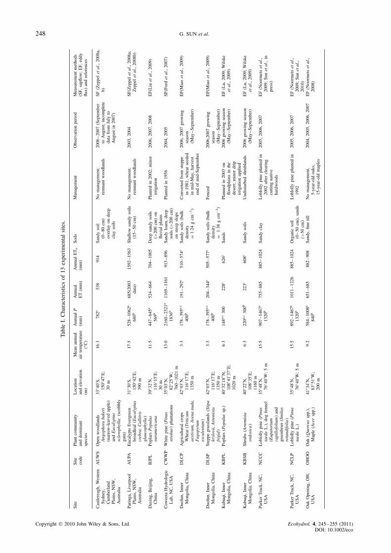
We assembled a database from 13 research sites that rep-resent a range of biomes. Sites span a large climatic gradi-ent, ranging from subtropical rain forests (CWWP) in thehumid Appalachians in the southeastern United States,to the hot dry woodlands in eastern Australia (AUWS,AUPA), and from forested wetlands (NCLP, NCCC) onthe Atlantic coastal plain in the southeastern United Statesto the grasslands (DLSP, XLDS, XLFC) and shrub lands(KBSB) and cultivated croplands (DLCP) in the semi-arid Inner Mongolia region in northern China (Figure 1;Table I). Management practices also vary widely. Thedata set includes two loblolly pine plantations (NCLP,NCCC) on a drained wetland landscape and two poplarplantation sites (BJPL, KBPL) that were subject to briefirrigation during the growing seasons. For the same grass-land ecosystem type, the data set consists of an ecosystemthat was under annual grazing (XLDS) and one underprotection (XLFC) from human disturbances (i.e. fenced,no grazing). The geographic range of the sites varies inlatitude from 43Ð5 °N to 33Ð7 °S and in longitude from83Ð8 °W to 150Ð8 °E. The annual mean air temperatureranges from 0Ð6 to 17Ð6 °C and mean annual precipitationfrom 300 to over 1800 mm year�1. Details of the physi-cal characteristics, site codes, research methods, and keyreferences that have published the ET data for each siteare listed in Table I.

Monthly total ET from each site was scaled fromhalf-hour measurements using either the standard eddycovariance methods or the sapflow and interceptionmethods (Table I). Although most of the ET data hadbeen published, ancillary data, such as monthly averagedLAI, P, and climatic variables, were assembled fromvarious sources.

To be consistent, we defined the growing seasonin the northern hemisphere to be May–September andOctober–April in the southern hemisphere. We acknowl-edge that there was no distinct growing season for thetwo Australian forests used here and the tree growth wasgenerally limited to water availability. As some sites didnot have year-round measurements, therefore, this studyfocused on growing season ET when cross-site compar-isons were made.

Calculated grass reference evapotranspiration (ETo)

Potential evapotranspiration (PET) is a nebulous termand can evoke confusion because PET does not clearlyspecify what land surface it refers to. For example,the ‘potential’ amount of water that a forest couldevaporate and transpire would be much higher thana grassland ecosystem could under the same ‘waterunlimited’ conditions due to the larger leaf area of theforest compared to the grassland. Thus, forest PET valuesshould be much higher than grassland PET under thesame climate. When the differences of PET methodsare ignored and a general PET method for grassland orcrops is used for a forest-dominated landscape, serious

Copyright 2010 John Wiley & Sons, Ltd. Ecohydrol. 4, 245–255 (2011)DOI: 10.1002/eco

A MODEL FOR ESTIMATING ECOSYSTEM EVAPOTRANSPIRATION 247

OakOpening, Toledo,Ohio(OHOO)

Beijing Poplar Plantation(BJPL)

DuolunSteppe (DLSP) , IM

XilinhotGrazed Grassland (XLDS),IM

Australia, Castlereagh,Western Sydney(AUWS)

Australia, Paringa, Open woodland (AUPA)White pine,Coweeta,

NC(CWWP

Loblolly pine(NCLP)

Clearcut(NCCC)

XilinhotFencedGrassland (XLSP),IM

KubuqiShrubland(KBSB),Inner Mongolia (IM)

KubuqiPoplar Plantation (KBPL) ,Inner Mongolia (IM)

DuolunCroplands (DLCP) , IM

Figure 1. Geographic distribution and characteristics of 13 ecosystems across a climatic and management gradient.

underestimation of actual forest ET is expected (Sunet al., 2010). To allay this confusion and normalizethe vegetated land surface to which PET refers to,the term grass reference ET (ETo) has gradually beenreplacing the PET term as a standard way to represent theenergy conditions for a particular region and makes PETestimates comparable worldwide (Allen et al., 1994).Using the process-based Penman-Monteith ET equation,actual daily ET of a hypothetical well-watered grass (i.e.ETo) that has a 0Ð12-m canopy height, a leaf area of 4Ð8,a bulk surface resistance of 70 s m�1, and an albedo of0Ð23 is estimated as follows:

ETo D 0Ð408�Rn � G� C ��C/�T C 273��u2�es � ea�

C ��1 C 0Ð34u2�,

�1�where ETo D grass reference ET (mm)

D slope of the saturation water vapour pressure atair temperature T (kPa °C�1)

D 2503e17Ð27T/�TC237Ð3�

�T C 237Ð3�2

Rn D net radiation (MJ m�2);G D soil heat flux (MJ m�2);� D the psychrometric constant (kPa °C�1);es D saturation vapour pressure (kPa);ea D actual vapour pressure (kPa);u2 D mean wind speed (m s�1) at 2 m height;C D unit conversion factor with a value of 900.

Details of the computation procedures are found in Allenet al. (1994). Monthly ETo rates were calculated as thesum of daily values in this study.

Empirical ET model development

We pooled all published data of monthly ET, P, andLAI that were measured onsite using various methods(Table I), and the monthly ETo estimated by Equation (1)as described above. The observation time length variedfrom one full growing season to 3 years (Table I). Thisdatabase contains 270 records (i.e. 270 site-months).All data analyses were performed using the SAS 9Ð2software (SAS Institute Inc., 2008). Regression modelsthat relate ET, ETo, P, and LAI for the entire data setwere developed using the SAS’s regression procedure.Different combinations of the independent variables (P,LAI, and ETo) were tested to derive the best fit ofobserved data. Influences of ETo, P, and LAI on ETfor each site were determined by the Pearson correlationcoefficients with significant level at ˛ D 0Ð05.

RESULTS

ETo, P, and ET in the growing season

The 13 sites covered a large range of climatic regimesas indicated by average air temperature and annual totalprecipitation (Table I), resulting in a large difference inecosystem structures (i.e. LAI) and water balance pat-terns. For example, the Coweeta site (CWWP) in the


248 G. SUN et al.

Tabl

eI.

Cha

ract

eris

tics

of13

expe

rim

enta

lsi

tes.

Site

Site

code

Plan

tco

mm

unity

and

dom

inan

tsp

ecie

s

Loc

atio

nan

del

evat

ion

(m)

Mea

nan

nual

air

tem

pera

ture

(°C

)

Ann

ual

P(m

m)

Ann

ual

ET

(mm

)A

nnua

lE

To

(mm

)So

ilsM

anag

emen

tO

bser

vatio

npe

riod

Mea

sure

men

tm

etho

ds(S

F,sa

pflow

;E

F,ed

dyflu

x)an

dre

fere

nces

Cas

tlere

agh,

Wes

tern

Sydn

ey,

Cum

berl

and

Pla

ins,

NS

W,

Aus

tral

ia

AU

WS

Ope

nw

oodl

ands

Ang

opho

raba

keri

(nar

row

-lea

ved

appl

e)an

dE

ucal

yptu

ssc

lero

phyl

la;

(scr

ibbl

ygu

m)

33° 4

00 S,

150°

470 E

;30

m

16Ð3

782a

538

914

Sand

yso

il(0

–80

cm)

over

lay

onde

epcl

ayso

ils

No

man

agem

ent;

rem

nant

woo

dlan

ds20

06–

2007

(Sep

tem

ber

toA

ugus

t;in

com

plet

eda

tafr

omJu

lyto

Aug

ust

in20

07)

SF(Z

eppe

let

al.,

2008

a,b)

Pari

nga,

Liv

erpo

olP

lain

s,N

SW

,A

ustr

alia

AU

PAE

ucal

ypts

Eve

rgre

enbr

oadl

eaf

(Euc

alyp

tus

creb

ra;

Cal

litr

isgl

auco

phyl

la)

31° 3

00 S,

150°

420 E

;39

0m

17Ð5

528

–10

62a

680b

685(

2003

data

)15

92–

1563

Sha

llow

sand

yso

ils(1

5–

50cm

)N

om

anag

emen

t;re

mna

ntw

oodl

ands

2003

,20

04SF

(Zep

pel

etal

.,20

08a;

Zep

pel

etal

.,20

08b)

Dax

ing,

Bei

jing,

Chi

naB

JPL

Pop

lars

Pop

ulus

eura

mer

ican

a39

° 320 N

,11

6°15

0 E;

30m

11Ð5

447

–64

5a

569b

524

–66

470

4–

1005

Dee

psa

ndy

soils

(>20

0cm

)on

fluvi

alpl

ains

Plan

ted

in20

02;

min

orir

riga

tion

2006

,20

07,

2008

EF(

Liu

etal

.,20

09)

Cow

eeta

Hyd

rolo

gic

Lab

,N

C,

USA

CW

WP

Whi

tepi

ne(P

inus

stro

bus)

plan

tatio

ns35

° 030 N

,82

° 250 W

;76

0–

1021

m

13Ð0

2160

–23

21a

1836

b11

69–

1161

913

–89

6Sa

ndy

loam

,de

epso

ils(>

200

cm)

onst

eep

slop

s

Plan

ted

in19

5620

04,

2005

SF(F

ord

etal

.,20

07)

Duo

lun,

Inne

rM

ongo

lia,

Chi

naD

LC

PA

gric

ultu

ral

crop

sW

heat

(Tri

ticu

mae

stiv

um,

Ave

nanu

da,

Fag

opyr

umes

cule

ntum

)

42° 0

30 N,

116°

170 E

;13

50m

3Ð317

8–

395a,

c

400b

191

–29

2c51

0–

574c

Sand

yso

ils(b

ulk

dens

ityD

1Ð24

gcm

�3)

Con

vert

edfr

omst

eppe

in19

81;

whe

atse

eded

inm

id-M

ay,

harv

est

end

ofm

id-S

epte

mbe

r

2006

,20

07gr

owin

gse

ason

(May

–S

epte

mbe

r)

EF(

Mia

oet

al.,

2009

)

Duo

lun,

Inne

rM

ongo

lia,

Chi

naD

LSP

Step

pegr

assl

ands

(Sti

pakr

ylov

ii,

Art

emis

iafr

igid

)

42° 0

30 N,

116°

170 E

;13

50m

3Ð317

8–

395a,

c

400b

204

–34

4c50

5–

577c

Sand

yso

ils(b

ulk

dens

ityD

1Ð38

gcm

�3)

Fenc

ed20

06,2

007

grow

ing

seas

on(M

ay–

Sep

tem

ber)

EF(

Mia

oet

al.,

2009

)

Kub

uqi,

Inne

rM

ongo

lia,

Chi

naK

BPL

Popl

ars

(Pop

ulus

sp.)

40° 3

20 1800 N

,10

8°41

0 3700 E

;10

20m

6Ð314

8a,c

300

228c

626c

Sand

sP

lann

edin

2003

onflo

odpl

ains

inth

ede

sert

;m

inor

drip

irri

gatio

nap

plie

d

2006

grow

ing

seas

on(M

ay–

Sep

tem

ber)

EF

(Lu,

2009

;W

ilske

etal

.,20

09)

Kub

uqi,

Inne

rM

ongo

lia,

Chi

naK

BSB

Shru

bs(A

rtem

isia

ordo

sica

)40

° 220 N

,10

8°35

0 E;

1160

m

6Ð322

0a,c

300b

223c

608c

Sand

yso

ilsU

ndis

turb

edsh

rubl

ands

2006

grow

ing

seas

on(M

ay–

Sep

tem

ber)

EF

(Lu,

2009

;W

ilske

etal

.,20

09)

Par

ker

Tra

ck,

NC

,U

SA

NC

CC

Lob

lolly

pine

(Pin

usta

eda

L.)

,do

gfe

nnel

(Eup

ator

ium

capi

llof

oliu

m)

and

gree

nbri

er(S

mil

axro

tund

ifol

ia)

35° 4

80 N,

76° 4

00 W;

5m

15Ð5

907

–14

67a

1320

b75

5–

885

885

–10

24S

andy

clay

Lob

lolly

pine

plan

ted

in20

02af

ter

clea

ring

cutti

ngna

tive

hard

woo

ds

2005

,20

06,

2007

EF

(Noo

rmet

set

al.,

2009

;S

unet

al.,

inpr

ess)

Par

ker

Tra

ck,

NC

,U

SA

NC

LP

Lob

lolly

pine

(Pin

usta

eda

L.)

35° 4

80 N,

76° 4

00 W;

5m

15Ð5

892

–14

67a

1320

b10

11–

1226

885

–10

24O

rgan

icso

il(0

–50

cm),

sand

s(>

50cm

)

Lob

lolly

pine

plan

ted

in19

9220

05,

2006

,20

07E

F(N

oorm

ets

etal

.,20

09;

Sun

etal

.,20

10)

Oak

Ope

ning

,O

H,

US

AO

HO

OO

ak(Q

uerc

ussp

p.),

Map

le(A

cer

spp.

)41

° 340 N

,83

° 510 W

;20

0m

9Ð258

4–

1008

a

840b

651

–68

588

2–

908

San

dy,

fine

till

No

man

agem

ent,

5-ye

ar-o

ldoa

ks;

15-y

ear-

old

map

les

2004

,20

05,

2006

,20

07E

F(N

oorm

ets

etal

.,20

08)



Tabl

eI.

(Con

tinu

ed).

Site

Site

code

Pla

ntco

mm

unity

and

dom

inan

tsp

ecie

s

Loc

atio

nan

del

evat

ion

(m)

Mea

nan

nual

air

tem

pera

ture

(°C

)

Ann

ual

P(m

m)

Ann

ual

ET

(mm

)A

nnua

lE

To

(mm

)So

ilsM

anag

emen

tO

bser

vatio

npe

riod

Mea

sure

men

tm

etho

ds(S

F,sa

pflow

;E

F,ed

dyflu

x)an

dre

fere

nces

Xili

nhot

,In

ner

Mon

golia

,C

hina

XL

DS

Deg

rade

dSt

eppe

gras

slan

ds(L

eym

usch

inen

sis,

Stip

akr

ylov

ii,

Art

emis

iafr

igid

)

43° 3

30 N,

116°

400 E

;12

50m

0Ð615

4–

184a,

c

350b

¾192

c60

8–

699c

Sand

yso

ils(b

ulk

dens

ityD

1Ð33

gcm

�3)

Und

erlo

ng-t

erm

graz

ing

2006

,200

7gr

owin

gse

ason

(May

–S

epte

mbe

r)

EF

(Mia

oet

al.,

2009

)

Xili

nhot

,In

ner

Mon

golia

,C

hina

XL

FCSt

eppe

gras

slan

ds(L

eym

usch

inen

sis,

Stip

agr

andi

s,A

rtem

isia

frig

id)

43° 3

30 N,

116°

400 E

;12

50m

0Ð615

4–

184a,

c

350b

¾190

c66

2–

708c

Sand

yso

ils(b

ulk

dens

ityD

1Ð22

gcm

�3)

Fenc

edin

2005

afte

rlo

ng-t

erm

graz

ing

2006

,20

07gr

owin

gse

ason

(May

–S

epte

mbe

r)

EF

(Mia

oet

al.,

2009

)

aPr

ecip

itatio

nlis

ted

deno

tes

the

rang

eor

tota

ldu

ring

the

stud

ype

riod

.b

Prec

ipita

tion

liste

dde

note

sth

era

nge

orto

tal

duri

ngth

elo

ng-t

erm

mea

n.c

Gro

win

gse

ason

(May

–Se

ptem

ber)

mea

sure

men

tson

ly.

southeastern United States had the highest annual pre-cipitation (>2000 mm) with a temperate climate, thussupported a plantation conifer forest with the highest LAI(peak LAI D 7Ð1) among all sites examined. In contrast,The Kubuqi shrub (KUSB) and poplar plantation (KUPL)sites in a desert environment of western China’s InnerMongolia had an annual precipitation of <300 mm andlow air temperature of 6Ð3 °C (Table I). Thus, those twosites supported plant communities with a low LAI (LAI< 0Ð4). The Paringa site on the Liverpool Plain in east-ern Australia had the highest annual ETo (¾1070 mm)and moderate annual precipitation (P D 680 mm) with arather high seasonal and annual variability. A combina-tion of high ETo and uneven distribution of rainfall mightexplain the periodic water stress that resulted in low LAI(maximum LAI < 1Ð3) for this water-limited ecosystem(Zeppel et al., 2006).

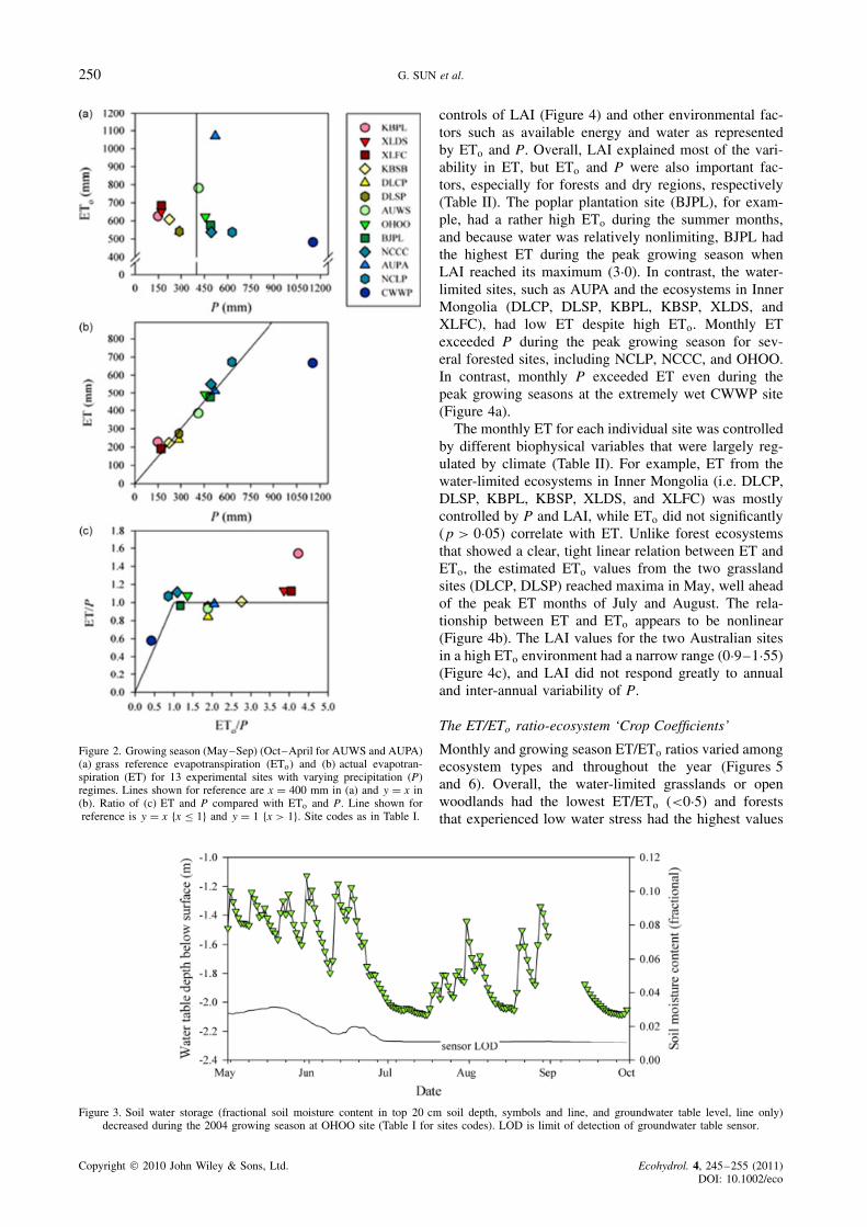
In addition to the contrasting differences in annualaveraged climate, the 13 sites had contrasting patternsof P and ETo during the growing seasons (Figure 2).The CWWP had the highest precipitation (1153 mm)but the lowest ETo (482 mm), while the KBPL receivedthe lowest precipitation (228 mm) and the AUPA hadthe highest ETo (1070 mm) (Figure 2a). Across the 13sites, it appears that the 400 mm precipitation line sep-arated the grassland ecosystems from temperate forestsand water-stressed open woodlands in eastern Australia(Figure 2a). Energy received by the grassland regions onthe Mongolian Plateau and other drier forest sites (Bei-jing and Toledo) were comparable to the forest sites inthe southeastern United States, suggesting that the aridand semi-humid ecosystems were not energy limited forET during the growing season, but rather limited by P.

The total growing season ET was linearly correlatedwith P (R2 D 0Ð96, p < 0Ð001) with a slope of 0Ð99, withCWWP being an exception (Figure 2b) to the overallrelationship as a group. Among the 13 sites, except for thewettest (CWWP) and driest (KUPL) sites, ET was within10% of P (Figure 2c). Precipitation barely matched theET demand at BJPL, AUWS, AUPA, DLSP, and KUSBand was less than ET at the NCLP, NCCC, OHOO,KUPL, XLDS, XLFC sites during the growing season.In contrast, the CWWP had the lowest ETo, but thehighest ET (Figures 2a–b). The CWWP received 50%more P (1153 mm) than needed for ET consumptionduring the growing season. Thus, severe droughts werenot likely for this site, and a perennial stream existedat this relatively wet site (ETo/P < 0Ð5) (Ford et al.,2007). Therefore, unlike the other 12 sites that weresomewhat water-limited as indicated by the aridity index(ETo/P), the CWWP was an energy-limited system. Thegroundwater table, an indicator of soil water storage,declined dramatically during the growing season at theNCLP, NCCC (Sun et al., 2010), and OHOO sites(Figure 3).

Monthly ETo, P, and ET

Monthly ET values varied from less than 10 mm month�1

to as high as 170 mm month�1, reflecting the biophysical


250 G. SUN et al.

Figure 2. Growing season (May–Sep) (Oct–April for AUWS and AUPA)(a) grass reference evapotranspiration (ETo) and (b) actual evapotran-spiration (ET) for 13 experimental sites with varying precipitation (P)regimes. Lines shown for reference are x D 400 mm in (a) and y D x in(b). Ratio of (c) ET and P compared with ETo and P. Line shown forreference is y D x fx � 1g and y D 1 fx > 1g. Site codes as in Table I.

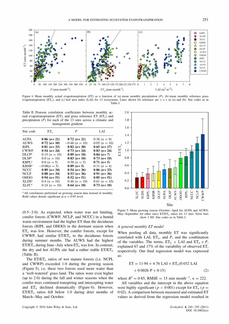
controls of LAI (Figure 4) and other environmental fac-tors such as available energy and water as representedby ETo and P. Overall, LAI explained most of the vari-ability in ET, but ETo and P were also important fac-tors, especially for forests and dry regions, respectively(Table II). The poplar plantation site (BJPL), for exam-ple, had a rather high ETo during the summer months,and because water was relatively nonlimiting, BJPL hadthe highest ET during the peak growing season whenLAI reached its maximum (3Ð0). In contrast, the water-limited sites, such as AUPA and the ecosystems in InnerMongolia (DLCP, DLSP, KBPL, KBSP, XLDS, andXLFC), had low ET despite high ETo. Monthly ETexceeded P during the peak growing season for sev-eral forested sites, including NCLP, NCCC, and OHOO.In contrast, monthly P exceeded ET even during thepeak growing seasons at the extremely wet CWWP site(Figure 4a).

The monthly ET for each individual site was controlledby different biophysical variables that were largely reg-ulated by climate (Table II). For example, ET from thewater-limited ecosystems in Inner Mongolia (i.e. DLCP,DLSP, KBPL, KBSP, XLDS, and XLFC) was mostlycontrolled by P and LAI, while ETo did not significantly(p > 0Ð05) correlate with ET. Unlike forest ecosystemsthat showed a clear, tight linear relation between ET andETo, the estimated ETo values from the two grasslandsites (DLCP, DLSP) reached maxima in May, well aheadof the peak ET months of July and August. The rela-tionship between ET and ETo appears to be nonlinear(Figure 4b). The LAI values for the two Australian sitesin a high ETo environment had a narrow range (0Ð9–1Ð55)(Figure 4c), and LAI did not respond greatly to annualand inter-annual variability of P.

The ET/ETo ratio-ecosystem ‘Crop Coefficients’

Monthly and growing season ET/ETo ratios varied amongecosystem types and throughout the year (Figures 5and 6). Overall, the water-limited grasslands or openwoodlands had the lowest ET/ETo (<0Ð5) and foreststhat experienced low water stress had the highest values

Figure 3. Soil water storage (fractional soil moisture content in top 20 cm soil depth, symbols and line, and groundwater table level, line only)decreased during the 2004 growing season at OHOO site (Table I for sites codes). LOD is limit of detection of groundwater table sensor.



Figure 4. Mean monthly actual evapotranspiration (ET) as a function of (a) mean monthly precipitation (P), (b) mean monthly reference grassevapotranspiration (ETo), and (c) leaf area index (LAI) for 13 ecosystems. Lines shown for reference are y D x in (a) and (b). Site codes as in

Table I.

Table II. Pearson correlation coefficients between monthly ac-tual evapotranspiration (ET), and grass reference ET (ETo) andprecipitation (P) for each of the 13 sites across a climatic and

management gradient.

Site code ETo P LAI

AUPA 0Ð86 (n= 21) 0Ð72 (n= 21) 0Ð36 (n D 9)AUWS 0Ð72 (n= 10) �0Ð46 (n D 10) 0Ð05 (n D 10)BJPL 0Ð81 (n= 33) 0Ð82 (n= 30) 0Ð65 (n= 17)CWWP 0Ð54 (n= 24) 0Ð73 (n= 24) 0Ð83 (n= 24)DLCPa 0Ð15 (n D 10) 0Ð89 (n= 10) 0Ð84 (n= 7)DLSPa 0Ð0 (n D 10) 0Ð83 (n= 10) 0Ð73 (n= 10)KBPLa 0Ð0 (n D 5) 0Ð58 (n D 5) 0Ð71 (n= 5)KBSBa �0Ð08(n D 5) 0Ð89 (n= 5) 0Ð31 (n D 4)NCCC 0Ð89 (n= 34) 0Ð54 (n= 36) 0Ð86 (n= 33)NCLP 0Ð88 (n= 34) 0Ð53 (n= 36) 0Ð91 (n= 36)OHOO 0Ð94 (n= 51) 0Ð52 (n= 51) 0Ð85 (n= 51)XLDSa 0Ð4 (n D 10) 0Ð46 (n D 10) 0Ð61 (n D 10)XLFCa 0Ð24 (n D 10) 0Ð64 (n= 10) 0Ð73 (n= 10)

a All correlations performed on growing season data instead of monthly.Bold values denote significant at ˛ D 0Ð05 level.

(0Ð5–2Ð0). As expected, when water was not limiting,conifer forests (CWWP, NCLP, and NCCC) in a humidwarm environment had the higher ET than the deciduousforests (BJPL and OHOO) in the dormant season whenETo was low. However, the conifer forests, except forCWWP, had similar ET/ETo to the deciduous forestsduring summer months. The AUWS had the highestET/ETo during June–July when ETo was low. In contrast,the dry and hot AUPA site had a rather stable ET/ETo

(Table II).The ET/ETo ratios of wet mature forests (i.e. NCPL

and CWWP) exceeded 1Ð0 during the growing season(Figure 5), i.e. these two forests used more water thana ‘well-watered’ grass land. The ratios were even higher(up to 2Ð0) during the fall and winter seasons when theconifer trees continued transpiring and intercepting waterand ETo declined dramatically (Figure 6). However,ET/ETo ratios fell below 1Ð0 during drier months ofMarch–May and October.

Figure 5. Mean growing season (October–April for AUPA and AUWS;May–September for other sites) ET/ETo ratios for 13 sites. Error bars

show 1 SD. Site codes as in Table I.

A general monthly ET model

When pooling all data, monthly ET was significantlycorrelated with LAI, ETo, and P, and the combinationof the variables. The terms, ETo ð LAI and ETo ð P,explained 67 and 17% of the variability of observed ET,respectively. Our final regression model was expressedas:

ET D 11Ð94 C 4Ð76 LAI C ETo�0Ð032 LAI

C 0Ð0026 P C 0Ð15� �2�

where R2 D 0Ð85, RMSE D 15 mm month�1, n D 222.All variables and the intercept in the above equation

were highly significant (p < 0Ð001) except for ETo (p D0Ð02). A comparison between measured and estimated ETvalues as derived from the regression model resulted in


252 G. SUN et al.

Figure 6. Mean monthly ratio of evapotranspiration (ET) to a grass reference evapotranspiration (ETo) for 13 sites. Error bars are 1 SD. Site codesas in Table I.

Figure 7. Predicted and measured monthly evapotranspiration (ET). Linesshown are modelled mean (solid) and prediction intervals for the mean

(dotted).

an overall RMSE of 15Ð1 mm month�1, representing anrelative error of 23% (Figure 7).

DISCUSSION

Relationships between ET, P, ETo, and LAI

At a long time scale, ecosystem ET is mainly controlledby the availability of evaporative energy (ETo) and waterinputs (P) and, to a minor extent, by vegetation types(Zhang et al., 2001, 2004; Lu et al., 2003; Oudin et al.,2008). The general relationships among ET, P, and ETo

for average climatic conditions have been well describedby Budyko-type of models (Zhang et al., 2004). Budykocurves show the relationship of E/P versus PET/P (i.e.aridity index). Theoretically, in energy-limited systemsthese two variables are linearly related to one anotherwith a slope of 1Ð0. In extremely water-limited systems,E/P approaches the limit of 1Ð0 over a long term.This suggests that ET/PET ratios for most ecosystems

should fall below the theoretical curve (Zhang et al.,2004), and ET can be estimated from the site levelaridity index (PET/P). However, finer temporal resolution(i.e. monthly or seasonal) information is required to aidin the water resource management decisions such aswater allocation during droughts or flooding mitigation.Ecosystem and water stresses on human water supplyoccur most often during periods with high water demandand low water supply, both supply and demand fluctuateseasonally, but normally reach the extremes during thegrowing season (Sun et al., 2008a).

This multiple-ecosystem synthesis study shows that thegeneral relationships among terrestrial water loss, energy,and water availability as outlined by Zhang et al. (2004)hold true. However, our study offers new insights onthe intricate relationships among precipitation, availabil-ity of evaporative energy, and vegetation dynamics at afiner temporal scale (i.e. monthly)—a scale that mostregional-scale hydrological models use for global changestudies (Vorosmarty et al., 1998; McNulty et al., 2010).By examining the empirical relations between ET andLAI across a range of ecosystems and temporal scales,this study confirmed that besides energy and water avail-ability, LAI is a critical variable for understanding andmodelling regional ET at a seasonal basis. LAI has beenwell known to be a good integrator of many biologi-cal and physiological controls on ET processes (Chapinet al., 2004); thus, this finding was not surprising. LAIdynamics affect land surface albedo (Betts, 2000; Sunet al., 2010), stand canopy total conductance (Zeppelet al., 2008b; Ford et al., 2010), canopy interception rates(Helvey, 1967; McCarthy et al., 1992), root biomass anddistribution (O’Grady et al., 2006), and the partitioningbetween evaporation and transpiration (Scott et al., 2006;Zhou et al., 2008). In fact, most process-based foresthydrological models (i.e. MIKE SHE) consider LAI as amajor control on daily or sub-daily ET (Lu et al., 2009).Plants respond to water stress through reducing stomatalconductance and/or LAI (Limousin et al., 2009). Zep-pel et al. (2008b) suggested that tree water use at theAustralian sites responded to water availability through



adjusting stomatal conductance, not LAI. A large portion(>50%) of the total ET loss for these types of woodlandswas by understory ET and canopy interception (Zeppelet al., 2008b).

Jackson et al. (2009) emphasized the hydrological sig-nificance of vegetation change due to human activitiessuch as afforestation or deforestation, especially in aridand semi-arid regions where ecohydrology is sensitiveto human disturbances and climatic change. Our studyoffered new evidence of the delicate balances betweenwater use, water yield, and vegetation structure for awide range of climatic and management regimes. Waterloss (ET) from most ecosystems examined in this studyconverged more or less around the amount of precipita-tion (P) received during the growing season. The growingseason ET of the young poplar plantation at the KUPLsite exceeded more than 50% of precipitation under anextremely dry environment (ETo/P > 4). Therefore, dripirrigation using groundwater as additional water sourceswas needed to support stand development (Lu et al.,2009; Wilske et al., 2009). For those sites where ETwas about 10% higher than P, shallow groundwater wasessential for NCLP, NCCC, and OHOO (Sun et al., 2010)and soil moisture was essential for XLDS and XLFC(Chen et al., 2009; Miao et al., 2009). Both sources ofwater represent water accumulated prior to the growingseason. Therefore, groundwater or soil storage systemslikely served as important reservoirs to meet peak ETdemand during the growing season for those systems.

The tight coupling between P and ET during the grow-ing season, and the fact that ET could slightly exceedP, even in forested wetlands (e.g. NCLP, NCCC) haveimportant implications for the ecosystem water balanceand its response to climatic variability. Both growing sea-son precipitation and soil water recharge in the nongrow-ing season were necessary for ecosystems to meet waterdemand in the growing season. Therefore, shifting sea-sonal precipitation patterns due to climate change couldprofoundly affect ecosystem water use patterns during thegrowing season, thus affecting the sustainability of somemanaged ecosystems. For example, a slight reductionin precipitation or increase in atmospheric evaporativedemand (e.g. climatic warming) could severely impactecosystems such as BJPL, KUSB, DLSP, SUPA, AUPA,and AUWS that were on the threshold of being underchronic seasonal water stress. While our synthesis studysuggests that rates of water loss from ecosystems con-verges on growing season precipitation, a larger samplesize and representation of vegetation types would be nec-essary to rigorously address this hypothesis.

Applications of the ET model

The accuracy of the ET model derived from this studyis sufficient for monthly hydrological forecasting at aregional scale as judged by the high R2 value (0Ð85)and moderate estimation error. However, future studiesshould include more diverse ecosystems to make theempirical model more applicable. For example, there

was a large data gap in terms of growing seasonprecipitation regime between 650 and 1150 mm, andbeyond 1150 mm in wet tropical regions (Figure 2). Asa result of the data gaps, it is unclear if the maximumgrowing seasonal ET found from this study (about700 mm during May–September) is the ET limit ofterrestrial forested ecosystems.

Although much advancement in the fields of remotesensing, global hydrological and climatic monitoring, andflux measurements has been made, accurately estimatingET for a large area remains challenging (Mu et al., 2007).The empirical ET model developed from our study hasthe potential to estimate regional ET using hybrid datasets that can be acquired from a combination of remotesensing and ground monitoring. For example, LAI, a keyinput to our model, is readily available at a relativelyhigh resolution (8 days, 500 m ð 500 m) from theModerate Resolution Imaging Spectroradiometer remotesensing products. Both ETo and P can be derivedfrom interpolated products from a network of weatherstations or projected climate change scenarios fromGlobal Circulation Models. When climatic variables suchas radiation, humidity, or wind speed are not available,ETo in our model should be estimated by the modifiedsimpler PET models (Lu et al., 2005) based on therelationship between ETo and PET.

Uncertainties

Estimating monthly ET is an imprecise science (Allen,2008) regardless of the estimation methods. For example,a š10% measurement error for energy fluxes as quan-tified by energy balance ratio (sum of latent heat andsensible heat divided by total available energy, i.e. netradiation minus soil heat flux) was not uncommon amongthe FLUXNET sites (Wilson et al., 2002). The energyclosure for our study sites ranged from 62% at the BJPLto 110% at the Inner Mongolia grassland sites. Likewise,the tree-based sapflow C canopy interception method forestimating ecosystem-level ET could contribute 7–14%of error when compared to watershed-scale water bal-ance method at the CWWP site (Ford et al., 2007). Thecanopy interception rate was high at this site, approxi-mately 45% of total ET. This component was not mea-sured directly but was rather modelled using an empiricalcanopy interception model (Ford et al., 2007). Up to 10%disparity between modelled tree transpiration and scaledup sapflux estimates were found for the AUPA in an anal-ysis by Zeppel et al. (2008b). For such sparsely vegetatedsites such as AUPA and AUWS, soil evaporation waslikely a large component of total ET, and canopy inter-ception estimates were uncertain (Zeppel et al., 2008b).In addition, measurement errors were possible in evenbasic landscape-scale hydrological and energy compo-nents, such as precipitation and net radiation. Errors forthese components can range as high as 9–20% (Barkeret al., 2009). Such measurement errors could result in alarge uncertainty in estimated monthly P and ETo. Werecognize that the current study may include some of


254 G. SUN et al.

the above errors, as well as errors associated with multi-ple site syntheses. Variations in instrumentation type anddata processing methodology (e.g. gap filling and scalingfrom 30-min measurements to daily and monthly val-ues) may all contribute to the uncertainty of reported ETdata. These errors may have contributed to the estimationerrors of the regression model that included 15% unex-plained elements other than P, ETo, and LAI. In addition,the six sites in Inner Mongolia had measurements onlyduring the growing seasons. Thus, the incomplete mea-surement cycles might cause bias towards the growingseasons and might miss important information regardingthe interactions of water and energy balances betweenthe nongrowing season and growing seasons that wereartificially set.

CONCLUSIONS

This synthesis study concludes that most of the variabilityof monthly ecosystem ET across a diverse climatic andmanagement gradient could be explained by leaf area(LAI), precipitation, and the availability of evaporativeenergy. The empirical ET model developed from thisstudy has the potential to be used for studying the regionalimpacts of climate and land cover change on seasonal ETand ecosystem water balances.

For most ecosystems examined, water use was close toprecipitation received during the growing season. There-fore, growing season precipitation is critical to meetingplant water demand. This implies that deviations from the‘norm’ in hydrological fluxes due to either precipitationreduction or increase in plant water consumption couldtip the water balances and result in the alteration of onsiteand offsite water flow and downstream water availabil-ity. Nongrowing season precipitation and water storagein soils and aquifers would affect streamflow and wateravailability in the growing season because precipitationwas roughly balanced by ET during the growing season.Future studies should include more eddy flux sites, suchas the FLUXNET that covers a wider climatic regime (i.e.wet tropics), to test the proposed hypotheses (i.e. grow-ing season ET convergence phenomena) and to refine theempirical model for wider applications.

The ET/ETo ratios varied seasonally and annually, andacross ecosystem types due to climatic variability andplant phenology. The ‘Crop Coefficient’ values offereda convenient way to empirically estimate ET when cli-matic data are available from local weather stations. Thisstudy offered additional evidence to show that temper-ate forests could use more water than ‘potential ET’ ofgrass ecosystems in a humid environment. The traditionalhydrological modelling approach that sets an ET limitusing potential ET (defined as the well-watered grass ref-erence ET) may cause large estimation errors, especiallyfor modelling ET for a forest-dominated landscape. Moreresearch is needed to develop standardized forest ver-sions of FAO Penman-Monteith models to account for thecomplexity of forest ecosystems in contrast to annualcrops or grasslands.

ACKNOWLEDGEMENTS

This study was supported by the USDA Forest ServiceEastern Forest Environmental Threat Assessment Centerand the Coweeta Hydrologic Laboratory. This study isalso partially supported by the United States-China Car-bon Consortium (USCCC), the Natural Science Founda-tion of China (30928002), and NASA-NEWS and NASALUCC Program (NNX09AM55G).

REFERENCES

Allen RG. 2008. Why do we care about ET? Southwest Hydrology 7:18–19.

Allen RG, Smith M, Perrier A, Pereira LS. 1994. An update for thedefinition of reference evapotranspiration. ICID Bulletin 43: 1–34.

Amatya DM, Trettin CC. 2007. Annual evapotranspiration of a forestedwetland watershed, SC. ASABE Paper No. 07222. In ASABE AnnualInternational Meeting . ASABE: St. Joseph, MI; 16.

Arain MA, Black TA, Barr AG, Griffis TJ, Morgenstern K, Nesic Z.2003. Year-round observations of the energy and water vapour fluxesabove a boreal black spruce forest. Hydrological Processes 17:3581–3600. DOI: 10.1002/hyp.1348.

Barker CA, Amiro BD, Kwon H, Ewers BE, Angstmann JL. 2009.Evapotranspiration in intermediate-aged and mature fens and uplandblack spruce boreal forests. Ecohydrology 2: 462–471. DOI:10.1002/eco.74.

Betts RA. 2000. Offset of the potential carbon sink from borealforestation by decreases in surface albedo. Nature 408: 187–190. DOI:10.1038/35041545.

Chapin FS III, Matson PA, Mooney HA. 2004. Principles of TerrestrialEcosystem Ecology . Springer: New York, NY; 472.

Chen S, Chen J, Lin G, Zhang W, Miao H, Wei L, Huang J, Han X.2009. Energy balance and partition in Inner Mongolia steppeecosystems with different land use types. Agricultural and ForestMeteorology 149: 1800–1809. DOI: 10.1016/j.agrformet.2009.06.009.

Currie DJ. 1991. Energy and large-scale patterns of animal- and plant-species richness. The American Naturalist 137: 27–49.

DeWalle DR, Swistock BR, Johnson TE, McGuire KJ. 2000. Potentialeffects of climate change and urbanization on mean annual streamflowin the United States. Water Resources Research 36: 2655–2664.

Ewers BE, Mackay DS, Gower ST, Ahl DE, Burrows SN, Samanta SS.2002. Tree species effects on stand transpiration in northern Wisconsin.Water Resources Research 38: 1103. DOI: 10.1029/2001WR000830.

Foley JA, DeFries R, Asner GP, Barford C, Bonan G, Carpenter SR,Chapin FS, Coe MT, Daily GC, Gibbs HK, Helkowski JH, Hol-loway T, Howard EA, Kucharik CJ, Monfreda C, Patz JA, Pren-tice IC, Ramankutty N, Snyder PK. 2005. Global consequences of landuse. Science 309: 570–574. DOI: 10.1126/science.1111772.

Ford CR, Hubbard RM, Kloeppel BD, Vose JM. 2007. A comparison ofsap flux-based evapotranspiration estimates with catchment-scale waterbalance. Agricultural and Forest Meteorology 145: 176–185. DOI:10.1016/j.agrformet.2007.04.010.

Ford CR, Hubbard RM, Vose JM. 2010. Quantifying structural andphysiological controls on canopy transpiration of planted pine andhardwood stand species in the southern Appalachians. Ecohydrology4: 2.

Hanson PJ, Amthor JS, Wullschleger SD, Wilson KB, Grant RF, Hart-ley A, Hui D, Hunt JER, Johnson DW, Kimball JS, King AW, Luo Y,McNulty SG, Sun G, Thornton PE, Wang S, Williams M, Baldoc-chi DD, Cushman RM. 2004. Oak forest carbon and water simulations:model intercomparisons and evaluations against independent data. Eco-logical Monographs 74: 443–489. DOI: 10.1890/03-4049.

Helvey JD. 1967. Interception by eastern white pine. Water ResourcesResearch 3: 723–729.

Jackson RB, Carpenter SR, Dahm CN, McKnight DM, Naiman RJ,Postel SL, Running SW. 2001. Water in a changing world.Ecological Applications 11: 1027–1045. DOI: 10.1890/1051-0761(2001)011[1027:WIACW]2.0.CO;2.

Jackson RB, Jobbagy EG, Avissar R, Roy SB, Barrett DJ, Cook CW,Farley KA, le Maitre DC, McCarl BA, Murray BC. 2005. Tradingwater for carbon with biological carbon sequestration. Science 310:1944–1947. DOI: 10.1126/science.1119282.

Jackson RB, Jobbagy EG, Nosetto MD. 2009. Ecohydrology in a human-dominated landscape. Ecohydrology 2: 383–389. DOI: 10.1002/eco.81.



Law BE, Falge E, Gu L, Baldocchi DD, Bakwin P, Berbigier P,Davis K, Dolman AJ, Falk M, Fuentes JD, Goldstein A, Granier A,Grelle A, Hollinger D, Janssens IA, Jarvis P, Jensen NO, Katul G,Mahli Y, Matteucci G, Meyers T, Monson R, Munger W, Oechel W,Olson R, Pilegaard K, Paw U KT, Thorgeirsson H, Valentini R,Verma S, Vesala T, Wilson K, Wofsy S. 2002. Environmental controlsover carbon dioxide and water vapor exchange of terrestrialvegetation. Agricultural and Forest Meteorology 113: 97–120. DOI:10.1016/S0168-1923(02)00104-1.

Limousin JM, Rambal S, Ourcival JM, Rocheteau A, Joffre R,Rodriguez-Cortina R. 2009. Long-term transpiration change withrainfall decline in a Mediterranean Quercus ilex forest. Global ChangeBiology 15: 2163–2175.

Liu C, Zhang Z, Sun G, Zhu J, Zha T, Shen L, Chen J, Fang X, Chen J.2009. Quantifying evapotranspiration and the biophysical regulationsof a poplar plantation assessed by eddy covariance and sap flowmethods (Chinese). Journal of Plant Ecology 33: 706–718.

Liu Y, Stanturf J, Lu H. 2008. Modeling the potential of the northernChina forest shelterbelt in improving hydroclimate conditions. Journalof the American Water Resources Association 44: 1176–1192. DOI:10.1111/j.1752-1688.2008.00240.x.

Lu N. 2009. Regional climate change and vegetation water relations inInner Mongolia—lessons learned within the NASA project “Effectsof land use change on the energy and water balance of the semi-arid region of Inner Mongolia, China”. PhD dissertation, University ofToledo, Toledo, USA.

Lu J, Sun G, McNulty SG, Amatya DM. 2003. Modeling actualevapotranspiration from forested watersheds across the southeasternUnited States. Journal of the American Water Resources Association39: 886–896. DOI: 10.1111/j.1752-1688.2003.tb04413.x.

Lu J, Sun G, McNulty SG, Amatya DM. 2005. A comparison ofsix potential evapotranspiration methods for regional use in thesoutheastern United States. Journal of the American Water ResourcesAssociation 41: 621–633. DOI: 10.1111/j.1752-1688.2005.tb03759.x.

Lu J, Sun G, McNulty SG, Comerford NB. 2009. Sensitivity of pineflatwoods hydrology to climate change and forest management inFlorida, USA. Wetlands 29: 826–836. DOI: 10.1672/07-162.1.

McCarthy EJ, Flewelling JW, Skaggs RW. 1992. Hydrologic model fordrained forest watershed. Journal of Irrigation and Drainage Engi-neering 118: 242–255. DOI: 10.1061/(ASCE)0733–9437(1992)118 : 2(242).

McNulty SG, Sun G, Moore Myers JA, Cohen EC. 2010. Robbing Peterto Pay Paul: Tradeoffs Between Ecosystem Carbon Sequestration andWater Yield. Presented at Watershed Management 2010, Madison,Wisconsin, August 23–27.

Miao H, Chen S, Chen J, Zhang W, Zhang P, Wei L, Han X, Lin G.2009. Cultivation and grazing altered evapotranspiration anddynamics in Inner Mongolia steppes. Agricultural and ForestMeteorology 149: 1810–1819. DOI: 10.1016/j.agrformet.2009.06.011.

Milly PCD. 1994. Climate, soil water storage, and the average annualwater balance. Water Resources Research 30: 2143–2156.

Mu Q, Heinsch FA, Zhao M, Running SW. 2007. Development of aglobal evapotranspiration algorithm based on MODIS and globalmeteorology data. Remote Sensing of Environment 111: 519–536. DOI:10.1016/j.rse.2007.04.015.

Noormets A, Ewers BE, Sun G, Mackay S, Zheng D, McNulty SG,Chen J. 2006. Water and carbon cycles in heterogeneous landscapes: anecosystem perspective. In Ecology of Hierarchical Landscapes: FromTheory to Application, Chen J, Saunders SC, Brosofske KD, Crow TR(eds). Nova Science Publishers, Inc.: New York; 89–123.

Noormets A, McNulty SG, DeForest JL, Sun G, Li Q, Chen J. 2008.Drought during canopy development can have lasting effect onannual carbon balance. New Phytologist 179: 818–828. DOI:10.1111/j.1469–8137.2008.02501.x.

Noormets A, McNulty SG, Gavazzi MJ, Sun G, Domec JC, King J,Chen J. 2009. Response of carbon fluxes to drought in a coastalplain loblolly pine forest. Global Change Biology 16: 272–287. DOI:10.1111/j.365–2486.009.01928.x.

O’Grady AP, Worledge D, Battaglia M. 2006. Above- and below-groundrelationships, with particular reference to fine roots, in a youngEucalyptus globulus (Labill.) stand in southern Tasmania. Trees 20:531–538.

Oudin L, Andreassian V, Lerat J, Michel C. 2008. Has land cover asignificant impact on mean annual streamflow? An internationalassessment using 1508 catchments. Journal of Hydrology 357:303–316. DOI: 10.1016/j.jhydrol.2008.05.021.

Paw U KT. 2006. Unifying biomicrometeorological measurements.Agricultural and Forest Meteorology 137: 121–122. DOI: 10.1016/j.agrformet.2006.03.004.

Scott RL, Huxman TE, Cable WL, Emmerich WE. 2006. Partitioning ofevapotranspiration and its relation to carbon dioxide exchange in aChihuahuan desert shrubland. Hydrological Processes 20: 3227–3243.DOI: 10.1002/hyp.6329.

Shuttleworth WJ. 2008. Evapotranspiration measurement methods.Southwest Hydrology 7: 22–23.

Sun G, McNulty SG, Myers JAM, Cohen EC. 2008a. Impacts of multiplestresses on water demand and supply across the southeastern UnitedStates. Journal of the American Water Resources Association 44:1441–1457. DOI: 10.1111/j.1752-1688.2008.00250.x.

Sun G, Noormets A, Chen J, McNulty SG. 2008b. Evapotranspirationestimates from eddy covariance towers and hydrologic modeling inmanaged forests in Northern Wisconsin, USA. Agricultural and ForestMeteorology 148: 257–267. DOI: 10.1016/j.agrformet.2007.08.010.

Sun G, Sun J, Zhou G. 2009. Water and carbon dynamics in selectedecosystems in China. Agricultural and Forest Meteorology 149:1789–1790. DOI: 10.1016/j.agrformet.2009.06.008.

Sun G, Noormets A, Gavazzi MJ, McNulty SG, Chen J, Domec JC,King JS, Amatya DM, Skaggs RW. 2010. Energy and water balanceof two contrasting loblolly pine plantations on the lower coastalplain of North Carolina, USA. Forest Ecology and Management 259:1299–1310.

Vorosmarty CJ, Federer CA, Schloss AL. 1998. Potential evaporationfunctions compared on US watersheds: possible implications forglobal-scale water balance and terrestrial ecosystem modeling. Journalof Hydrology 207: 147–169. DOI: 10.1016/S0022-1694(98)00109-7.

Wang Y, Yu P, Feger KH, Wei X, Sun G, Bonell M, Xiong W, Zhang S,Xu L. Annual runoff and evapotranspiration of forestlands andnon-forestlands in selected basins of the Loess Plateau of China.Ecohydrology 4: 2.

Wilske B, Lu N, Wei L, Chen S, Zha T, Liu C, Xu W, Noormets A,Huang J, Wei Y, Chen J, Zhang Z, Ni J, Sun G, Guo K, McNulty SG,John R, Han X, Lin G, Chen J. 2009. Poplar plantation has thepotential to alter water balance in semiarid Inner Mongolia. Journal ofEnvironmental Management 90: 2762–1770.

Wilson K, Goldstein A, Falge E, Aubinet M, Baldocchi D, Berbigier P,Bernhofer C, Ceulemans R, Dolman H, Field C, Grelle A, Ibrom A,Law BE, Kowalski A, Meyers T, Moncrieff J, Monson R, Oechel W,Tenhunen J, Valentini R, Verma S. 2002. Energy balance closure atFLUXNET sites. Agricultural and Forest Meteorology 113: 223–243.DOI: 10.1016/S0168-1923(02)00109-0.

Wilson KB, Hanson PJ, Mulholland PJ, Baldocchi DD, Wullschleger SD.2001. A comparison of methods for determining forest evapotranspira-tion and its components: sap-flow, soil water budget, eddy covarianceand catchment water balance. Agricultural and Forest Meteorology106: 153–168. DOI: 10.1016/S0168-1923(00)00199-4.

Wullschleger SD, Meinzer FC, Vertessy RA. 1998. A review of whole-plant water use studies in tree. Tree Physiology 18: 499–512. DOI:10.1093/treephys/18.8– 9.499.

Zeppel MJB, Yunusa IAM, Eamus D. 2006. Daily, seasonal and annualpatterns of transpiration from a stand of remnant vegetationdominated by a coniferous Callitris species and a broad-leaved Euca-lyptus species. Physiologia Plantarum 127: 413–422. DOI:10.1111/j.1399–3054.2006.00674.x.

Zeppel M, Mcacinnis-Ng CMO, Ford CR, Eamus D. 2008a. Theresponse of sap flow to pulses of rain in a temperate Australianwoodland. Plant and Soil 305: 121–130.

Zeppel MJB, Macinnis-Ng CMO, Yunusa IAM, Whitley RJ, Eamus D.2008b. Long term trends of stand transpiration in a remnant forestduring wet and dry years. Journal of Hydrology 349: 200–213. DOI:10.1016/j.jhydrol.2007.11.001.

Zhang L, Dawes WR, Walker GR. 2001. Response of mean annualevapotranspiration to vegetation changes at catchment scale. WaterResources Research 37: 701–708.

Zhang L, Hickel K, Dawes WR, Chiew FHS, Western AW, Briggs PR.2004. A rational function approach for estimating mean annualevapotranspiration. Water Resources Research 40: W02502. DOI:10.1029/2003WR002710.

Zhou G, Sun G, Wang X, Zhou C, McNulty SG, Vose JM, Amatya DM.2008. Estimating forest ecosystem evapotranspiration at multipletemporal scales with a dimension analysis approach. Journal ofthe American Water Resources Association 44: 208–221. DOI:10.1111/j.1752-1688.2007.00148.x.


A general predictive model for estimating monthly ecosystem evapotranspiration

Documents