Outline Method I: Perturbation and Scaled Cook’s Distance Method II: Sensitivity Analysis Acknowledgement A General Framework for Model Diagnostics: Diagnostic Measures and Influence Analysis Hongtu Zhu Department of Biostatistics and Biomedical Research Imaging Center The University of North Carolina at Chapel Hill August 22, 2012 1 / 98

Welcome message from author
This document is posted to help you gain knowledge. Please leave a comment to let me know what you think about it! Share it to your friends and learn new things together.
Transcript

OutlineMethod I: Perturbation and Scaled Cook’s Distance
Method II: Sensitivity AnalysisAcknowledgement
A General Framework for Model Diagnostics:Diagnostic Measures and Influence Analysis
Hongtu Zhu
Department of Biostatistics and Biomedical Research Imaging CenterThe University of North Carolina at Chapel Hill
August 22, 2012
1 / 98
OutlineMethod I: Perturbation and Scaled Cook’s Distance
Method II: Sensitivity AnalysisAcknowledgement
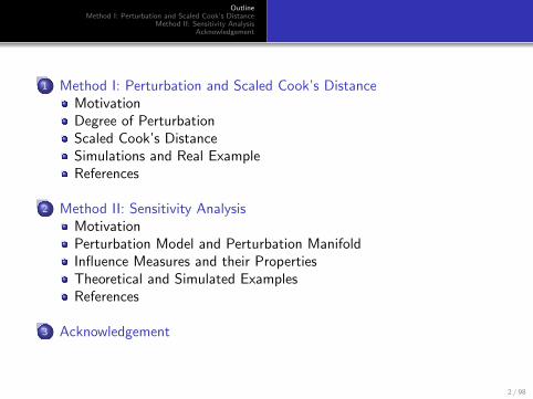
1 Method I: Perturbation and Scaled Cook’s DistanceMotivationDegree of PerturbationScaled Cook’s DistanceSimulations and Real ExampleReferences
2 Method II: Sensitivity AnalysisMotivationPerturbation Model and Perturbation ManifoldInfluence Measures and their PropertiesTheoretical and Simulated ExamplesReferences
3 Acknowledgement
2 / 98

OutlineMethod I: Perturbation and Scaled Cook’s Distance
Method II: Sensitivity AnalysisAcknowledgement
MotivationDegree of PerturbationScaled Cook’s DistanceSimulations and Real ExampleReferences
Motivation
Figure: True complicated process, Data, and ‘Right’/‘Fitted’ model.3 / 98
OutlineMethod I: Perturbation and Scaled Cook’s Distance
Method II: Sensitivity AnalysisAcknowledgement
MotivationDegree of PerturbationScaled Cook’s DistanceSimulations and Real ExampleReferences
Motivation
Data may come from a true complicated process.
Finding a ‘right’/‘fitted’ model to interpret a dataset and toapproximate the true complicated process.
Fitted Model 6= True Process
Discrepancy = Fitted ModelTrue Process
How do we use statistical tools (or diagnostic measures) to detectsuch discrepancies?
4 / 98
OutlineMethod I: Perturbation and Scaled Cook’s Distance
Method II: Sensitivity AnalysisAcknowledgement
MotivationDegree of PerturbationScaled Cook’s DistanceSimulations and Real ExampleReferences
Motivation
Discrepancy exists between isolated observations (e.g., influentialpoints and outliers) and the rest of the observations
residualsleveragescase-deletion measures
Any systematic discrepancies between the data and the fitted valuesobtained from statistical models
graphical procedures of residuals, such as partial residual and addedvariable plotsgoodness-of-fit test statistics and test procedures for testing specificalternativessensitivity analysis
5 / 98
OutlineMethod I: Perturbation and Scaled Cook’s Distance
Method II: Sensitivity AnalysisAcknowledgement
MotivationDegree of PerturbationScaled Cook’s DistanceSimulations and Real ExampleReferences
Motivation
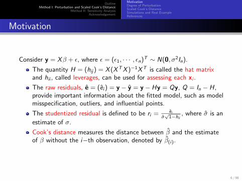
Consider y = Xβ + ε, where ε = (ε1, · · · , εn)T ∼ N(0, σ2In).
The quantity H = (hij) = X (XTX )−1XT is called the hat matrixand hii , called leverages, can be used for assessing each xi .
The raw residuals, e = (ei ) = y − y = y − Hy = Qy, Q = In − H,provide important information about the fitted model, such as modelmisspecification, outliers, and influential points.
The studentized residual is defined to be ri = eiσ√
1−hii, where σ is an
estimate of σ.
Cook’s distance measures the distance between β and the estimateof β without the i−th observation, denoted by β(i).
6 / 98
OutlineMethod I: Perturbation and Scaled Cook’s Distance
Method II: Sensitivity AnalysisAcknowledgement
MotivationDegree of PerturbationScaled Cook’s DistanceSimulations and Real ExampleReferences
Motivation
Most diagnostic measures were originally developed under linearregression models (Cook, 1977; Cook and Weisberg, 1982;Chatterjee and Hadi, 1988).
Considerable research has been devoted to developing diagnosticmeasures for generalized linear models and models for survival data(Andersen, 1992, Davison and Tsai, 1992; Wei, 1998; Storer andCrowley, 1985; Therneau, Grambsch, and Fleming, 1990; Lin, Wei,and Ying, 1993).
Diagnostic measures have been developed for various models forclustered data and models for missing data (Christensen et al., 1992;Preisser and Qaqish, 1996; Banerjee and Frees,1997; Haslett, 1999;Zhu, et al. 2001; Fung, et.al, 2002).
7 / 98

OutlineMethod I: Perturbation and Scaled Cook’s Distance
Method II: Sensitivity AnalysisAcknowledgement
MotivationDegree of PerturbationScaled Cook’s DistanceSimulations and Real ExampleReferences
Figure: Residual Analysis
8 / 98
OutlineMethod I: Perturbation and Scaled Cook’s Distance
Method II: Sensitivity AnalysisAcknowledgement
MotivationDegree of PerturbationScaled Cook’s DistanceSimulations and Real ExampleReferences
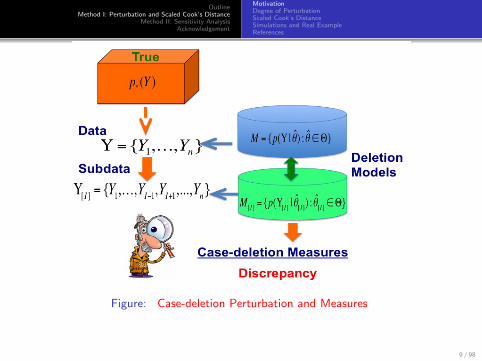
Figure: Case-deletion Perturbation and Measures
9 / 98
OutlineMethod I: Perturbation and Scaled Cook’s Distance
Method II: Sensitivity AnalysisAcknowledgement
MotivationDegree of PerturbationScaled Cook’s DistanceSimulations and Real ExampleReferences
Motivation
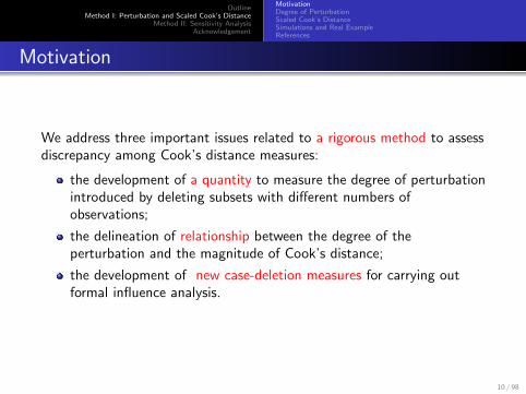
We address three important issues related to a rigorous method to assessdiscrepancy among Cook’s distance measures:
the development of a quantity to measure the degree of perturbationintroduced by deleting subsets with different numbers ofobservations;
the delineation of relationship between the degree of theperturbation and the magnitude of Cook’s distance;
the development of new case-deletion measures for carrying outformal influence analysis.
10 / 98

OutlineMethod I: Perturbation and Scaled Cook’s Distance
Method II: Sensitivity AnalysisAcknowledgement
MotivationDegree of PerturbationScaled Cook’s DistanceSimulations and Real ExampleReferences
Cook’s Distance
Consider YT = (Y T1 , . . . ,Y
Tn ) and p(Y|θ), where θ ∈ Θ ⊂ Rq.
The dimension of Yi = (yi,1, . . . , yi,mi ) may vary significantly acrossall i .
Let subscript ‘[I]’ denote the relevant quantity with all observationsin a set I deleted.
Let Y[I ] be a subsample of Y with YI = Y(i,j) : (i , j) ∈ I deletedand p(Y[I ]|θ) be its probability function.
θ = argmaxθ log p(Y|θ) and θ[I ] = argmaxθ log p(Y[I ]|θ);
CD(I ) = (θ[I ] − θ)TGnθ(θ[I ] − θ).
11 / 98
OutlineMethod I: Perturbation and Scaled Cook’s Distance
Method II: Sensitivity AnalysisAcknowledgement
MotivationDegree of PerturbationScaled Cook’s DistanceSimulations and Real ExampleReferences
Cook’s Distance
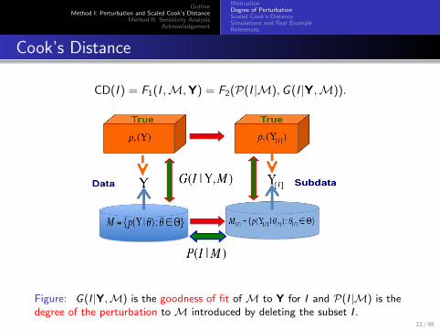
CD(I ) = F1(I ,M,Y) = F2(P(I |M),G (I |Y,M)).
Figure: G(I |Y,M) is the goodness of fit of M to Y for I and P(I |M) is thedegree of the perturbation to M introduced by deleting the subset I .
12 / 98

OutlineMethod I: Perturbation and Scaled Cook’s Distance
Method II: Sensitivity AnalysisAcknowledgement
MotivationDegree of PerturbationScaled Cook’s DistanceSimulations and Real ExampleReferences
Degree of Perturbation
Our choice of P(I |M) is motivated by five principles as follows.
(P.a) (non-negativity) For any subset I , P(I |M) is alwaysnon-negative.
(P.b) (uniqueness) P(I |M) = 0 if and only if I is an empty set.
(P.c) (monotonicity) If I2 ⊂ I1, then P(I2|M) ≤ P(I1|M).
(P.d) (additivity) If I2 ⊂ I1, I1·2 = I1 − I2, andp(YI1·2 |Y[I1],θ) = p(YI1·2 |Y[I1·2],θ) for all θ, then we haveP(I1|M) = P(I2|M) + P(I1·2|M).
(P.e) P(I |M) should naturally arise from the current model M, thedata Y, and the subset I .
13 / 98
OutlineMethod I: Perturbation and Scaled Cook’s Distance
Method II: Sensitivity AnalysisAcknowledgement
MotivationDegree of PerturbationScaled Cook’s DistanceSimulations and Real ExampleReferences
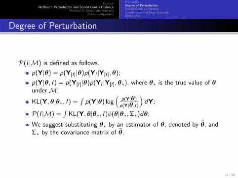
Degree of Perturbation
P(I |M) is defined as follows.
p(Y|θ) = p(Y[I ]|θ)p(YI |Y[I ],θ);
p(Y|θ, I ) = p(Y[I ]|θ)p(YI |Y[I ],θ∗), where θ∗ is the true value of θunder M;
KL(Y,θ|θ∗, I ) =∫
p(Y|θ) log(
p(Y|θ)
p(Y|θ,I )
)dY;
P(I |M) =∫
KL(Y,θ|θ∗, I )φ(θ|θ∗,Σ∗)dθ;
We suggest substituting θ∗ by an estimator of θ, denoted by θ, andΣ∗ by the covariance matrix of θ.
14 / 98

OutlineMethod I: Perturbation and Scaled Cook’s Distance
Method II: Sensitivity AnalysisAcknowledgement
MotivationDegree of PerturbationScaled Cook’s DistanceSimulations and Real ExampleReferences
Degree of Perturbation
Theorem 1. Suppose that L(Y : p(YI |Y[I ],θ) = p(YI |Y[I ],θ∗)) > 0for any θ 6= θ∗, where L(A) is the Lebesgue measure of a set A. Then,P(I |M) defined above satisfies the five principles (P.a)-(P.e).
15 / 98
OutlineMethod I: Perturbation and Scaled Cook’s Distance
Method II: Sensitivity AnalysisAcknowledgement
MotivationDegree of PerturbationScaled Cook’s DistanceSimulations and Real ExampleReferences
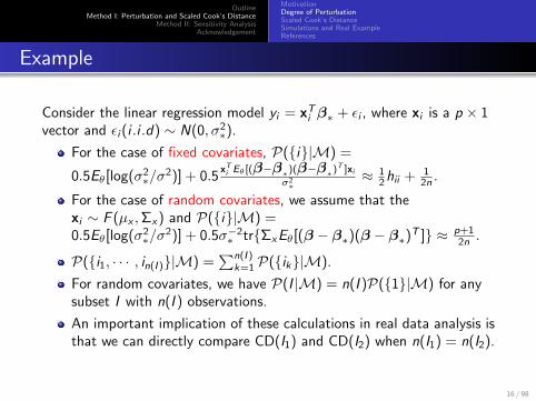
Example
Consider the linear regression model yi = xTi β∗ + εi , where xi is a p × 1vector and εi (i .i .d) ∼ N(0, σ2
∗).
For the case of fixed covariates, P(i|M) =
0.5Eθ[log(σ2∗/σ
2)] + 0.5xTi Eθ [(β−β∗)(β−β∗)T ]xi
σ2∗
≈ 12 hii + 1
2n .
For the case of random covariates, we assume that thexi ∼ F (µx ,Σx) and P(i|M) =0.5Eθ[log(σ2
∗/σ2)] + 0.5σ−2
∗ trΣxEθ[(β − β∗)(β − β∗)T ] ≈ p+12n .
P(i1, · · · , in(I )|M) =∑n(I )
k=1 P(ik|M).
For random covariates, we have P(I |M) = n(I )P(1|M) for anysubset I with n(I ) observations.
An important implication of these calculations in real data analysis isthat we can directly compare CD(I1) and CD(I2) when n(I1) = n(I2).
16 / 98
OutlineMethod I: Perturbation and Scaled Cook’s Distance
Method II: Sensitivity AnalysisAcknowledgement
MotivationDegree of PerturbationScaled Cook’s DistanceSimulations and Real ExampleReferences
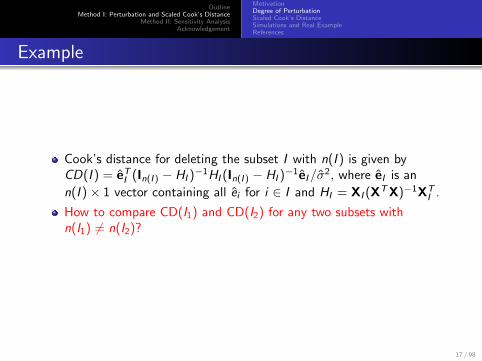
Example
Cook’s distance for deleting the subset I with n(I ) is given byCD(I ) = eT
I (In(I ) − HI )−1HI (In(I ) − HI )
−1eI/σ2, where eI is an
n(I )× 1 vector containing all ei for i ∈ I and HI = XI (XTX)−1XTI .
How to compare CD(I1) and CD(I2) for any two subsets withn(I1) 6= n(I2)?
17 / 98
OutlineMethod I: Perturbation and Scaled Cook’s Distance
Method II: Sensitivity AnalysisAcknowledgement
MotivationDegree of PerturbationScaled Cook’s DistanceSimulations and Real ExampleReferences
Example
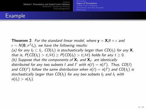
Theorem 2. For the standard linear model, where y = Xβ + ε andε ∼ N(0, σ2In), we have the following results:(a) for any I2 ⊂ I1, CD(I1) is stochastically larger than CD(I2) for any X,that is, P(CD(I1) > t|M) ≥ P(CD(I2) > t|M) holds for any t ≥ 0.(b) Suppose that the components of XI and XI ′ are identicallydistributed for any two subsets I and I ′ with n(I ) = n(I ′). Thus, CD(I )and CD(I ′) follow the same distribution when n(I ) = n(I ′) and CD(I1) isstochastically larger than CD(I2) for any two subsets I2 and I1 withn(I1) > n(I2).
18 / 98
OutlineMethod I: Perturbation and Scaled Cook’s Distance
Method II: Sensitivity AnalysisAcknowledgement
MotivationDegree of PerturbationScaled Cook’s DistanceSimulations and Real ExampleReferences
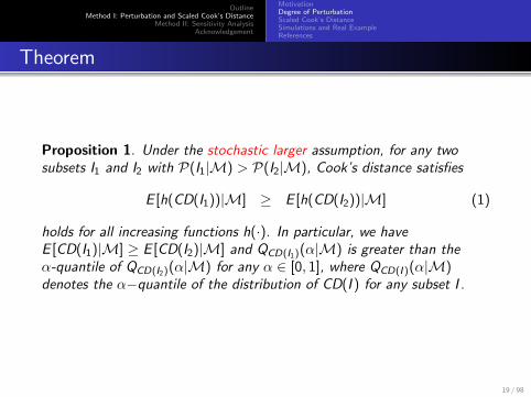
Theorem
Proposition 1. Under the stochastic larger assumption, for any twosubsets I1 and I2 with P(I1|M) > P(I2|M), Cook’s distance satisfies
E [h(CD(I1))|M] ≥ E [h(CD(I2))|M] (1)
holds for all increasing functions h(·). In particular, we haveE [CD(I1)|M] ≥ E [CD(I2)|M] and QCD(I1)(α|M) is greater than theα-quantile of QCD(I2)(α|M) for any α ∈ [0, 1], where QCD(I )(α|M)denotes the α−quantile of the distribution of CD(I ) for any subset I .
19 / 98
OutlineMethod I: Perturbation and Scaled Cook’s Distance
Method II: Sensitivity AnalysisAcknowledgement
MotivationDegree of PerturbationScaled Cook’s DistanceSimulations and Real ExampleReferences
Definition
Definition 1. The scaled Cook’s distances for matching (mean, Std) and(median, Mstd) are, respectively, defined as
SCD1(I ) =CD(I )− E [CD(I )|M]
Std[CD(I )|M]and SCD2(I ) =
CD(I )− QCD(I )(0.5|M)
Mstd[CD(I )|M],
where both the expectation and the quantile are taken with respect toM.Definition 2. The conditionally scaled Cook’s distances (CSCD) formatching (mean, Std) and (median, Mstd) while controlling for Z are,respectively, defined as
CSCD1(I ,Z) =CD(I )− E [CD(I )|M,Z]
Std[CD(I )|M,Z],
CSCD2(I ,Z) =CD(I )− QCD(I )(0.5|M,Z)
Mstd[CD(I )|M,Z],
where Z is the set of some fixed covariates in Y and the expectation andquantiles are taken with respect to M given Z.
20 / 98
OutlineMethod I: Perturbation and Scaled Cook’s Distance
Method II: Sensitivity AnalysisAcknowledgement
MotivationDegree of PerturbationScaled Cook’s DistanceSimulations and Real ExampleReferences
First-order Approximation
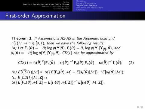
Theorem 3. If Assumptions A2-A5 in the Appendix hold andn(I )/n→ γ ∈ [0, 1), then we have the following results:(a) Let Fn(θ) = −∂2
θ log p(Y|θ), fI (θ) = ∂θ log p(YI |Y[I ], θ), andsI (θ) = −∂2
θ log p(YI |Y[I ],θ), CD(I ) can be approximated by
CD(I ) = fI (θ)T [Fn(θ)− sI (θ)]−1Fn(θ)[Fn(θ)− sI (θ)]−1fI (θ); (2)
(b) E [CD(I )|M] ≈ tr(E [Fn(θ)|M]− E [sI (θ)|M]−1E [sI (θ)|M]);
(c) E [CD(I )|M,Z] ≈tr(E [Fn(θ)|M,Z]− E [sI (θ)|M,Z]−1E [sI (θ)|M,Z]).
21 / 98
OutlineMethod I: Perturbation and Scaled Cook’s Distance
Method II: Sensitivity AnalysisAcknowledgement
MotivationDegree of PerturbationScaled Cook’s DistanceSimulations and Real ExampleReferences
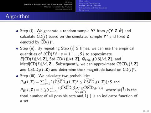
Algorithm
Step (i). We generate a random sample Ys from p(Y|Z, θ) and
calculate CD(I ) based on the simulated sample Ys and fixed Z,
denoted by CD(I )s .
Step (ii). By repeating Step (i) S times, we can use the empirical
quantities of CD(I )s : s = 1, . . . ,S to approximateE [CD(I )|M,Z], Std[CD(I )|M,Z], QCD(I )(0.5|M,Z), andMstd[CD(I )|M,Z]. Subsequently, we can approximate CSCD1(I ,Z)
and CSCD2(I ,Z) and determine their magnitude based on CD(I )s .
Step (iii). We calculate two probabilities
PA(I ,Z) =∑S
s=1 1(CSCD1(I ,Z)s ≤ CSCD1(I ,Z))/S and
PB(I ,Z) =∑
I
∑Ss=1
1(CSCD1(I ,Z)s≤CSCD1(I ,Z))
S×#(I ), where #(I ) is the
total number of all possible sets and 1(·) is an indicator function ofa set.
22 / 98
OutlineMethod I: Perturbation and Scaled Cook’s Distance
Method II: Sensitivity AnalysisAcknowledgement
MotivationDegree of PerturbationScaled Cook’s DistanceSimulations and Real ExampleReferences
Simulations
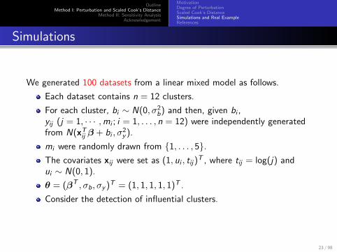
We generated 100 datasets from a linear mixed model as follows.
Each dataset contains n = 12 clusters.
For each cluster, bi ∼ N(0, σ2b) and then, given bi ,
yij (j = 1, · · · ,mi ; i = 1, . . . , n = 12) were independently generatedfrom N(xTij β + bi , σ
2y ).
mi were randomly drawn from 1, . . . , 5.The covariates xij were set as (1, ui , tij)
T , where tij = log(j) andui ∼ N(0, 1).
θ = (βT , σb, σy )T = (1, 1, 1, 1, 1)T .
Consider the detection of influential clusters.
23 / 98
OutlineMethod I: Perturbation and Scaled Cook’s Distance
Method II: Sensitivity AnalysisAcknowledgement
MotivationDegree of PerturbationScaled Cook’s DistanceSimulations and Real ExampleReferences
Simulations
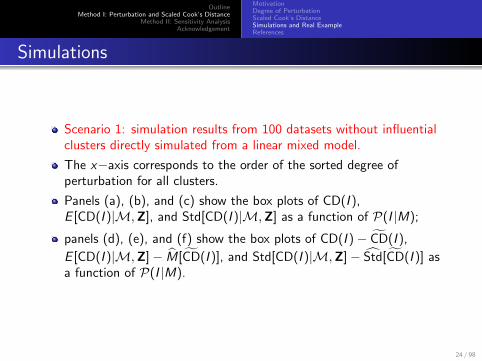
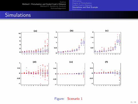
Scenario 1: simulation results from 100 datasets without influentialclusters directly simulated from a linear mixed model.
The x−axis corresponds to the order of the sorted degree ofperturbation for all clusters.
Panels (a), (b), and (c) show the box plots of CD(I ),E [CD(I )|M,Z], and Std[CD(I )|M,Z] as a function of P(I |M);
panels (d), (e), and (f) show the box plots of CD(I )− CD(I ),
E [CD(I )|M,Z]− M[CD(I )], and Std[CD(I )|M,Z]− Std[CD(I )] asa function of P(I |M).
24 / 98
OutlineMethod I: Perturbation and Scaled Cook’s Distance
Method II: Sensitivity AnalysisAcknowledgement
MotivationDegree of PerturbationScaled Cook’s DistanceSimulations and Real ExampleReferences
Simulations
Figure: Scenario 125 / 98

OutlineMethod I: Perturbation and Scaled Cook’s Distance
Method II: Sensitivity AnalysisAcknowledgement
MotivationDegree of PerturbationScaled Cook’s DistanceSimulations and Real ExampleReferences
Simulations
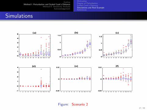
Scenario 2: Simulation results from 100 datasets with two influentialclusters simulated from a linear mixed model.
We reset (m1, b1) = (1, 4) and (mn, bn) = (5, 3) to generate yi,j fori = 1, n and all j according to the same linear mixed model.
The x−axis corresponds to the order of the sorted degree ofperturbation for all clusters.
Panels (a), (b), and (c) show the box plots of CD(I ),E [CD(I )|M,Z], and Std[CD(I )|M,Z] as a function of P(I |M);
panels (d), (e), and (f) show the box plots of CD(I )− CD(I ),
E [CD(I )|M,Z]− M[CD(I )], and Std[CD(I )|M,Z]− Std[CD(I )] asa function of P(I |M).
26 / 98
OutlineMethod I: Perturbation and Scaled Cook’s Distance
Method II: Sensitivity AnalysisAcknowledgement
MotivationDegree of PerturbationScaled Cook’s DistanceSimulations and Real ExampleReferences
Simulations
Figure: Scenario 227 / 98
OutlineMethod I: Perturbation and Scaled Cook’s Distance
Method II: Sensitivity AnalysisAcknowledgement
MotivationDegree of PerturbationScaled Cook’s DistanceSimulations and Real ExampleReferences
Simulations
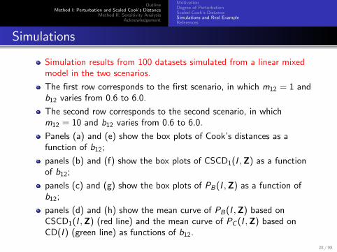
Simulation results from 100 datasets simulated from a linear mixedmodel in the two scenarios.
The first row corresponds to the first scenario, in which m12 = 1 andb12 varies from 0.6 to 6.0.
The second row corresponds to the second scenario, in whichm12 = 10 and b12 varies from 0.6 to 6.0.
Panels (a) and (e) show the box plots of Cook’s distances as afunction of b12;
panels (b) and (f) show the box plots of CSCD1(I ,Z) as a functionof b12;
panels (c) and (g) show the box plots of PB(I ,Z) as a function ofb12;
panels (d) and (h) show the mean curve of PB(I ,Z) based onCSCD1(I ,Z) (red line) and the mean curve of PC (I ,Z) based onCD(I ) (green line) as functions of b12.
28 / 98
OutlineMethod I: Perturbation and Scaled Cook’s Distance
Method II: Sensitivity AnalysisAcknowledgement
MotivationDegree of PerturbationScaled Cook’s DistanceSimulations and Real ExampleReferences
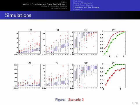
Simulations
Figure: Scenario 329 / 98

OutlineMethod I: Perturbation and Scaled Cook’s Distance
Method II: Sensitivity AnalysisAcknowledgement
MotivationDegree of PerturbationScaled Cook’s DistanceSimulations and Real ExampleReferences
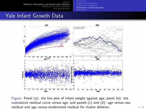
Yale Infant Growth Data
Study whether cocaine exposure during pregnancy may lead to themaltreatment of infants after birth.
A total of 298 children were recruited from cocaine exposed groupand unexposed group.∑n
i=1 mi = 3176, whereas mi varies from 2 to 30.
yi,j = xTi,jβ + εi,j , where yi,j is the weight (in kilograms) of the j-thvisit from the i-th subject, xi,j =(1, di,j , (di,j − 120)+, (di,j − 200)+, (gi − 28)+, di,j(gi − 28)+, (di,j −60)+(gi − 28)+, (di,j − 490)+(gi − 28)+, sidi,j , si (di,j − 120)+)T , inwhich di,j and gi (days) are the age of visit and gestational age,respectively, and si is the indicator for gender.
εi = (εi,1, . . . , εi,mi )T ∼ Nmi (0,Ri (α)).
M1: Ri (α) = α0Imi + α11⊗2mi
.
M2: V (d) = exp(α0 + α1d + α2d2 + α3d3) and ρ(l) = α4 + α5l ,where l is the lag between two visits.
30 / 98
OutlineMethod I: Perturbation and Scaled Cook’s Distance
Method II: Sensitivity AnalysisAcknowledgement
MotivationDegree of PerturbationScaled Cook’s DistanceSimulations and Real ExampleReferences
Yale Infant Growth Data
Figure: Panel (a): the line plot of infant weight against age; panel (b): thecumulative residual curve versus age; and panels (c) and (d): age versus rawresidual and age versus studentized residual for cluster deletion. 31 / 98
OutlineMethod I: Perturbation and Scaled Cook’s Distance
Method II: Sensitivity AnalysisAcknowledgement
MotivationDegree of PerturbationScaled Cook’s DistanceSimulations and Real ExampleReferences
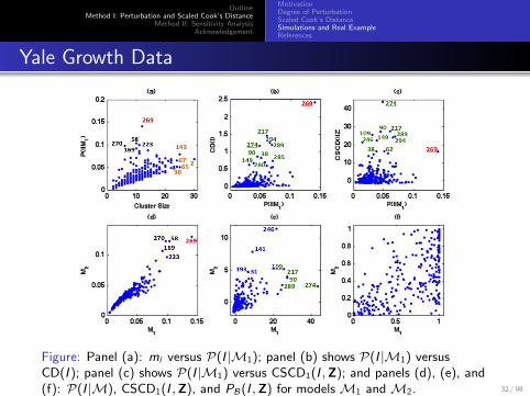
Yale Growth Data
Figure: Panel (a): mi versus P(I |M1); panel (b) shows P(I |M1) versusCD(I ); panel (c) shows P(I |M1) versus CSCD1(I ,Z); and panels (d), (e), and(f): P(I |M), CSCD1(I ,Z), and PB(I ,Z) for models M1 and M2. 32 / 98
OutlineMethod I: Perturbation and Scaled Cook’s Distance
Method II: Sensitivity AnalysisAcknowledgement
MotivationDegree of PerturbationScaled Cook’s DistanceSimulations and Real ExampleReferences
Yale Growth Data
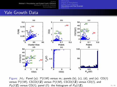
Figure: M1: Panel (a): P(I |M) versus mi ; panels (b), (c), (d), and (e): CD(I )versus P(I |M), CSCD(I |Z) versus P(I |M), CSCD(I |Z) versus CD(I ), andPB(I |Z) versus CD(I ); panel (f): the histogram of PB(I |Z). 33 / 98
OutlineMethod I: Perturbation and Scaled Cook’s Distance
Method II: Sensitivity AnalysisAcknowledgement
MotivationDegree of PerturbationScaled Cook’s DistanceSimulations and Real ExampleReferences
Yale Growth Data
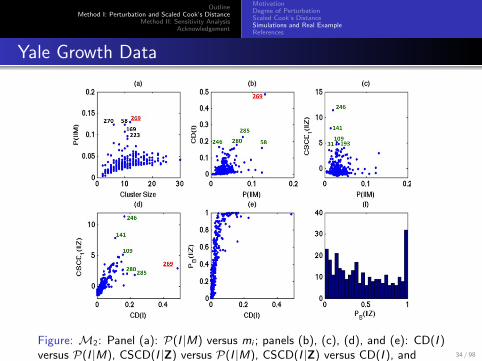
Figure: M2: Panel (a): P(I |M) versus mi ; panels (b), (c), (d), and (e): CD(I )versus P(I |M), CSCD(I |Z) versus P(I |M), CSCD(I |Z) versus CD(I ), andPB(I |Z) versus CD(I ); panel (f): the histogram of PB(I |Z).
34 / 98
OutlineMethod I: Perturbation and Scaled Cook’s Distance
Method II: Sensitivity AnalysisAcknowledgement
MotivationDegree of PerturbationScaled Cook’s DistanceSimulations and Real ExampleReferences
References
Zhu, HT., Ibrahim JG, Cho HS. Perturbation and scaled Cook’s distance.Annals of Statistics, 40, 785-811, 2012.
Zhu, HT, Ibrahim JG., Cho HS, and Tang, N.S. Bayesian case-deletionmeasures for statistical models with missing data, Journal ofComputational and Graphical Statistics, in press, 2012.
Zhu HT, Ibrahim, JG., Shi, X.Y. Diagnostic measures for generalizedlinear models with missing covariates. Scandivian Journal of Statistics, 36,686-712, 2009.
Cho HS, Ibrahim JG, Sinha and Zhu HT. Bayesian Case InfluenceDiagnostics for Survival Models, Biometrics, 65, 116-124, 2009.
Zhu HT, Tang NS, Ibrahim JG, and Zhang HP. Diagnostic measures forempirical likelihood of general estimating equations. Biometrika, 95,489-507, 2008.
Zhu HT, Lee SY, Wei BC, and Zhou JL. Case-deletion measures formodels with incomplete data. Biometrika, 88:727-737, 2001.
35 / 98

OutlineMethod I: Perturbation and Scaled Cook’s Distance
Method II: Sensitivity AnalysisAcknowledgement
MotivationPerturbation Model and Perturbation ManifoldInfluence Measures and their PropertiesTheoretical and Simulated ExamplesReferences
Motivation
Bayesian inference about a parameter θ is typically based oncalculating and summarizing the posterior distribution
p(θ|Dobs) =p(θ)p(Dobs |θ)∫p(θ)p(Dobs |θ)dθ
. (3)
It is well known that posterior quantities, such as the Bayes factor,posterior mean, etc... for a given dataset may be sensitive to anyperturbation to the three key elements of a Bayesian analysis: Dobs ,p(θ) and p(Dobs |θ).
In the Bayesian literature, various methods for sensitivity analysishave been developed to perturb each of these three key elementsand to assess the influence of various perturbations on the posteriordistribution and its associated posterior quantities.
36 / 98
OutlineMethod I: Perturbation and Scaled Cook’s Distance
Method II: Sensitivity AnalysisAcknowledgement
MotivationPerturbation Model and Perturbation ManifoldInfluence Measures and their PropertiesTheoretical and Simulated ExamplesReferences
Motivation
There are two major formal sensitivity techniques including theglobal and local robustness approaches (Berger, 1994).
The key idea of the global robustness approach is to compute therange of posterior quantities as the perturbation to each of the threekey elements change in a certain set of distributions and thendetermine the “extremal” ones (Berger, 1990).
The conditional predictive ordinate (CPO) and the Kullback-Leiblerdivergence are two global influence measures for assessing individualobservations.
The Bayes factor can be regarded as a global sensitivity method.
All these global sensitivity methods are generally computationallyintensive for high-dimensional parameters.
37 / 98
OutlineMethod I: Perturbation and Scaled Cook’s Distance
Method II: Sensitivity AnalysisAcknowledgement
MotivationPerturbation Model and Perturbation ManifoldInfluence Measures and their PropertiesTheoretical and Simulated ExamplesReferences
Motivation
The local robustness approach primarily computes the derivatives ofthe posterior quantities with respect to a small perturbation to p(θ)or p(Dobs |θ).
In the frequentist literature, Cook’s (1986) seminal local influenceapproach is particularly useful for perturbing p(Dobs |θ) in order todetect influential observations and assessing model misspecification.
In the Bayesian literature, an analogue of Cook’s (1986) approachhas been developed (Gustafson, 1996; Gustafson and Wasserman,1995; McCulloch, 1989; Berger, 1994; Berger, Insua, and Ruggeri,2000).
38 / 98
OutlineMethod I: Perturbation and Scaled Cook’s Distance
Method II: Sensitivity AnalysisAcknowledgement
MotivationPerturbation Model and Perturbation ManifoldInfluence Measures and their PropertiesTheoretical and Simulated ExamplesReferences
Motivation
Very little has been done on developing a general Bayesian influenceapproach for simultaneously perturbing Dobs , p(θ) and p(Dobs |θ),assessing their effects, and examining their applications in severalsettings, such as settings with missing data.
Clarke and Gustafson (1998) is the sole paper on simultaneouslyperturbing (Dobs , p(θ), p(Dobs |θ)) in the context of independent andidentically distributed data.
39 / 98
OutlineMethod I: Perturbation and Scaled Cook’s Distance
Method II: Sensitivity AnalysisAcknowledgement
MotivationPerturbation Model and Perturbation ManifoldInfluence Measures and their PropertiesTheoretical and Simulated ExamplesReferences
Motivation
We address three important issues related to the Bayesian influenceapproach:
the development of a perturbation model that unifies variousperturbation schemes for individually or simultaneously perturbing(Dobs , p(θ), p(Dobs |θ));
the development of a Bayesian perturbation manifold to characterizethe intrinsic structure of the perturbation model;
the development of local influence measures for selecting the mostinfluential perturbation based on various objective functions andtheir statistical properties;
the development of global influence measures for carrying outsensitivity analysis in missing data problem.
40 / 98
OutlineMethod I: Perturbation and Scaled Cook’s Distance
Method II: Sensitivity AnalysisAcknowledgement
MotivationPerturbation Model and Perturbation ManifoldInfluence Measures and their PropertiesTheoretical and Simulated ExamplesReferences
Perturbation Model
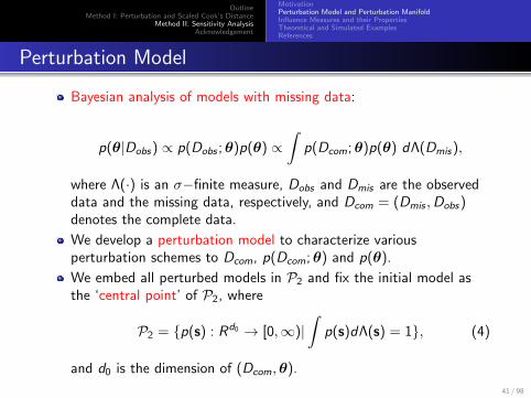
Bayesian analysis of models with missing data:
p(θ|Dobs) ∝ p(Dobs ;θ)p(θ) ∝∫
p(Dcom;θ)p(θ) dΛ(Dmis),
where Λ(·) is an σ−finite measure, Dobs and Dmis are the observeddata and the missing data, respectively, and Dcom = (Dmis ,Dobs)denotes the complete data.
We develop a perturbation model to characterize variousperturbation schemes to Dcom, p(Dcom;θ) and p(θ).
We embed all perturbed models in P2 and fix the initial model asthe ‘central point’ of P2, where
P2 = p(s) : Rd0 → [0,∞)|∫
p(s)dΛ(s) = 1, (4)
and d0 is the dimension of (Dcom,θ).
41 / 98
OutlineMethod I: Perturbation and Scaled Cook’s Distance
Method II: Sensitivity AnalysisAcknowledgement
MotivationPerturbation Model and Perturbation ManifoldInfluence Measures and their PropertiesTheoretical and Simulated ExamplesReferences
Perturbation Model
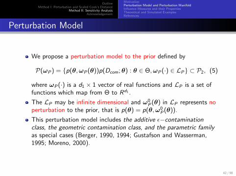
We propose a perturbation model to the prior defined by
P(ωP) = p(θ,ωP(θ))p(Dcom;θ) : θ ∈ Θ,ωP(·) ∈ LP ⊂ P2, (5)
where ωP(·) is a d1 × 1 vector of real functions and LP is a set offunctions which map from Θ to Rd1 .
The LP may be infinite dimensional and ω0P(θ) in LP represents no
perturbation to the prior, that is p(θ) = p(θ,ω0P(θ)).
This perturbation model includes the additive ε−contaminationclass, the geometric contamination class, and the parametric familyas special cases (Berger, 1990, 1994; Gustafson and Wasserman,1995; Moreno, 2000).
42 / 98
OutlineMethod I: Perturbation and Scaled Cook’s Distance
Method II: Sensitivity AnalysisAcknowledgement
MotivationPerturbation Model and Perturbation ManifoldInfluence Measures and their PropertiesTheoretical and Simulated ExamplesReferences
Perturbation Model
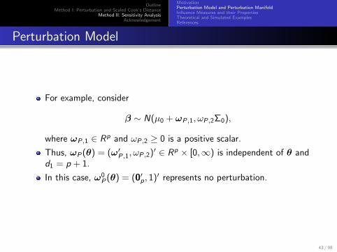
For example, consider
β ∼ N(µ0 + ωP,1, ωP,2Σ0),
where ωP,1 ∈ Rp and ωP,2 ≥ 0 is a positive scalar.
Thus, ωP(θ) = (ω′P,1, ωP,2)′ ∈ Rp × [0,∞) is independent of θ andd1 = p + 1.
In this case, ω0P(θ) = (0′p, 1)′ represents no perturbation.
43 / 98
OutlineMethod I: Perturbation and Scaled Cook’s Distance
Method II: Sensitivity AnalysisAcknowledgement
MotivationPerturbation Model and Perturbation ManifoldInfluence Measures and their PropertiesTheoretical and Simulated ExamplesReferences
Perturbation Model
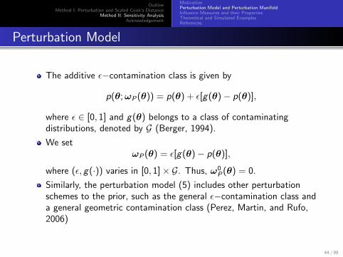
The additive ε−contamination class is given by
p(θ;ωP(θ)) = p(θ) + ε[g(θ)− p(θ)],
where ε ∈ [0, 1] and g(θ) belongs to a class of contaminatingdistributions, denoted by G (Berger, 1994).
We setωP(θ) = ε[g(θ)− p(θ)],
where (ε, g(·)) varies in [0, 1]× G. Thus, ω0P(θ) = 0.
Similarly, the perturbation model (5) includes other perturbationschemes to the prior, such as the general ε−contamination class anda general geometric contamination class (Perez, Martin, and Rufo,2006)
44 / 98
OutlineMethod I: Perturbation and Scaled Cook’s Distance
Method II: Sensitivity AnalysisAcknowledgement
MotivationPerturbation Model and Perturbation ManifoldInfluence Measures and their PropertiesTheoretical and Simulated ExamplesReferences
Data and Sampling Distribution
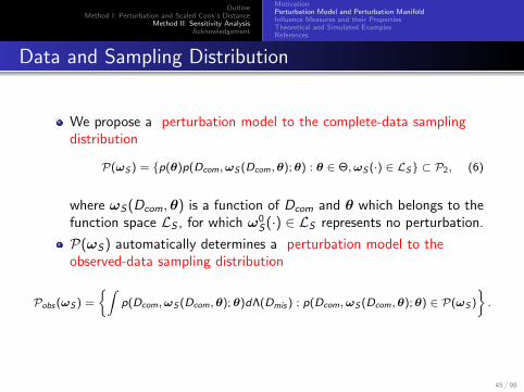
We propose a perturbation model to the complete-data samplingdistribution
P(ωS ) = p(θ)p(Dcom,ωS (Dcom,θ);θ) : θ ∈ Θ,ωS (·) ∈ LS ⊂ P2, (6)
where ωS(Dcom,θ) is a function of Dcom and θ which belongs to thefunction space LS , for which ω0
S(·) ∈ LS represents no perturbation.
P(ωS) automatically determines a perturbation model to theobserved-data sampling distribution
Pobs(ωS ) =
∫p(Dcom,ωS (Dcom,θ);θ)dΛ(Dmis) : p(Dcom,ωS (Dcom,θ);θ) ∈ P(ωS )
.
45 / 98
OutlineMethod I: Perturbation and Scaled Cook’s Distance
Method II: Sensitivity AnalysisAcknowledgement
MotivationPerturbation Model and Perturbation ManifoldInfluence Measures and their PropertiesTheoretical and Simulated ExamplesReferences
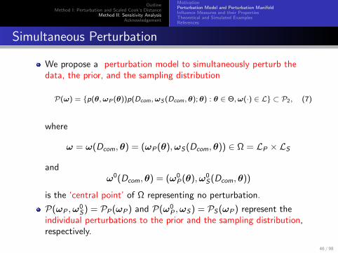
Simultaneous Perturbation
We propose a perturbation model to simultaneously perturb thedata, the prior, and the sampling distribution
P(ω) = p(θ,ωP(θ))p(Dcom,ωS (Dcom,θ);θ) : θ ∈ Θ,ω(·) ∈ L ⊂ P2, (7)
where
ω = ω(Dcom,θ) = (ωP(θ),ωS(Dcom,θ)) ∈ Ω = LP × LS
andω0(Dcom,θ) = (ω0
P(θ),ω0S(Dcom,θ))
is the ‘central point’ of Ω representing no perturbation.
P(ωP ,ω0S) = PP(ωP) and P(ω0
P ,ωS) = PS(ωP) represent theindividual perturbations to the prior and the sampling distribution,respectively.
46 / 98
OutlineMethod I: Perturbation and Scaled Cook’s Distance
Method II: Sensitivity AnalysisAcknowledgement
MotivationPerturbation Model and Perturbation ManifoldInfluence Measures and their PropertiesTheoretical and Simulated ExamplesReferences
Simultaneous Perturbation
Based on the perturbation model (7), we can measure the amountof perturbation, the extent to which each component of aperturbation model contributes to, and the degree of orthogonalityfor the components of the perturbation model.
Such a quantification is very useful for rigorously assessing therelative influence of each component in a Bayesian analysis, whichcan reveal any discrepancy among data, the prior, or the samplingmodel.
For instance, a data-prior discrepancy can arise when either anestimate of the parameter is in a low probability region of the prioror the prior leads to an improper posterior distribution.
Because the components of the perturbation model may not beorthogonal to each other, special care should be taken when weinterpret local influence measures from such a perturbation.
47 / 98
OutlineMethod I: Perturbation and Scaled Cook’s Distance
Method II: Sensitivity AnalysisAcknowledgement
MotivationPerturbation Model and Perturbation ManifoldInfluence Measures and their PropertiesTheoretical and Simulated ExamplesReferences
Bayesian Perturbation Manifold
We develop a Bayesian perturbation manifold (BPM) to measureeach perturbation ω in the perturbation model and apply thismethodology to a wide variety of statistical models, allowing forincomplete-data.
The perturbation model M = p(Dcom,θ;ω) : ω ∈ Ω has a naturalgeometrical structure. Since Ω can be either a finite dimensional setor an infinite dimensional set, we need to develop a manifold forinfinite dimensional space, which includes the finite dimensionalmanifold as a submanifold.
For instance, Ω for the ε−contamination class and the linearperturbation class are infinite dimensional, whereas Ω for theparametric family are finite dimensional.
48 / 98
OutlineMethod I: Perturbation and Scaled Cook’s Distance
Method II: Sensitivity AnalysisAcknowledgement
MotivationPerturbation Model and Perturbation ManifoldInfluence Measures and their PropertiesTheoretical and Simulated ExamplesReferences
Bayesian Perturbation Manifold
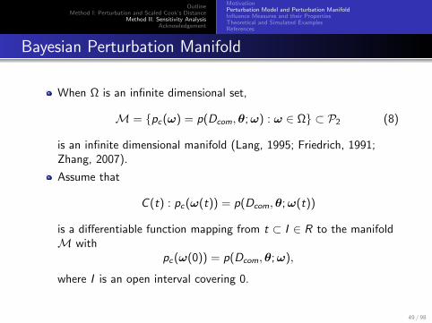
When Ω is an infinite dimensional set,
M = pc(ω) = p(Dcom,θ;ω) : ω ∈ Ω ⊂ P2 (8)
is an infinite dimensional manifold (Lang, 1995; Friedrich, 1991;Zhang, 2007).
Assume that
C (t) : pc(ω(t)) = p(Dcom,θ;ω(t))
is a differentiable function mapping from t ⊂ I ∈ R to the manifoldM with
pc(ω(0)) = p(Dcom,θ;ω),
where I is an open interval covering 0.
49 / 98
OutlineMethod I: Perturbation and Scaled Cook’s Distance
Method II: Sensitivity AnalysisAcknowledgement
MotivationPerturbation Model and Perturbation ManifoldInfluence Measures and their PropertiesTheoretical and Simulated ExamplesReferences
Bayesian Perturbation Manifold
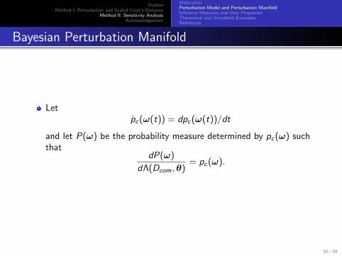
Letpc(ω(t)) = dpc(ω(t))/dt
and let P(ω) be the probability measure determined by pc(ω) suchthat
dP(ω)
dΛ(Dcom,θ)= pc(ω).
50 / 98
OutlineMethod I: Perturbation and Scaled Cook’s Distance
Method II: Sensitivity AnalysisAcknowledgement
MotivationPerturbation Model and Perturbation ManifoldInfluence Measures and their PropertiesTheoretical and Simulated ExamplesReferences
Bayesian Perturbation Manifold
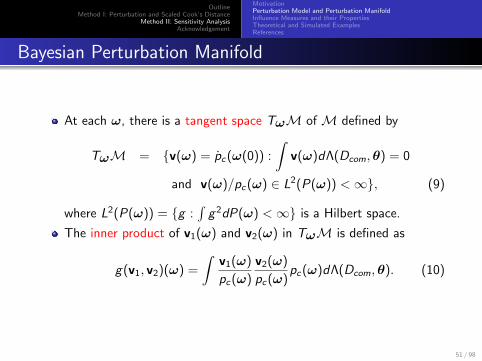
At each ω, there is a tangent space TωM of M defined by
TωM = v(ω) = pc(ω(0)) :
∫v(ω)dΛ(Dcom,θ) = 0
and v(ω)/pc(ω) ∈ L2(P(ω)) <∞, (9)
where L2(P(ω)) = g :∫
g 2dP(ω) <∞ is a Hilbert space.
The inner product of v1(ω) and v2(ω) in TωM is defined as
g(v1, v2)(ω) =
∫v1(ω)
pc(ω)
v2(ω)
pc(ω)pc(ω)dΛ(Dcom,θ). (10)
51 / 98
OutlineMethod I: Perturbation and Scaled Cook’s Distance
Method II: Sensitivity AnalysisAcknowledgement
MotivationPerturbation Model and Perturbation ManifoldInfluence Measures and their PropertiesTheoretical and Simulated ExamplesReferences
Bayesian Perturbation Manifold
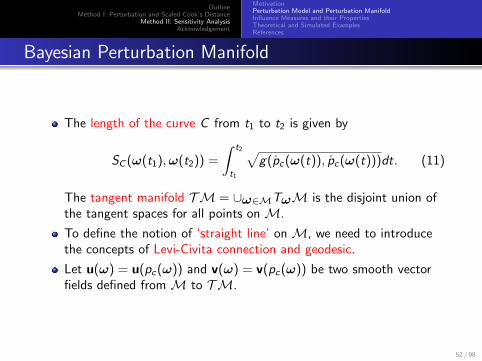
The length of the curve C from t1 to t2 is given by
SC (ω(t1),ω(t2)) =
∫ t2
t1
√g(pc(ω(t)), pc(ω(t)))dt. (11)
The tangent manifold TM = ∪ω∈MTωM is the disjoint union ofthe tangent spaces for all points on M.
To define the notion of ‘straight line’ on M, we need to introducethe concepts of Levi-Civita connection and geodesic.
Let u(ω) = u(pc(ω)) and v(ω) = v(pc(ω)) be two smooth vectorfields defined from M to TM.
52 / 98
OutlineMethod I: Perturbation and Scaled Cook’s Distance
Method II: Sensitivity AnalysisAcknowledgement
MotivationPerturbation Model and Perturbation ManifoldInfluence Measures and their PropertiesTheoretical and Simulated ExamplesReferences
Bayesian Perturbation Manifold
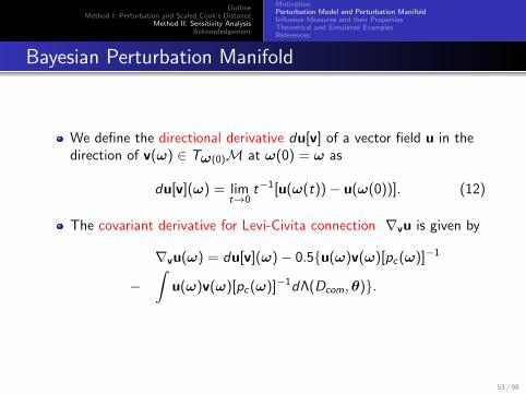
We define the directional derivative du[v] of a vector field u in thedirection of v(ω) ∈ Tω(0)M at ω(0) = ω as
du[v](ω) = limt→0
t−1[u(ω(t))− u(ω(0))]. (12)
The covariant derivative for Levi-Civita connection ∇vu is given by
∇vu(ω) = du[v](ω)− 0.5u(ω)v(ω)[pc(ω)]−1
−∫
u(ω)v(ω)[pc(ω)]−1dΛ(Dcom,θ).
53 / 98
OutlineMethod I: Perturbation and Scaled Cook’s Distance
Method II: Sensitivity AnalysisAcknowledgement
MotivationPerturbation Model and Perturbation ManifoldInfluence Measures and their PropertiesTheoretical and Simulated ExamplesReferences
Bayesian Perturbation Manifold
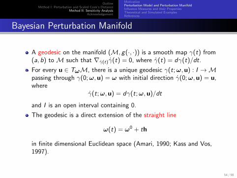
A geodesic on the manifold (M, g(·, ·)) is a smooth map γ(t) from(a, b) to M such that ∇γ(t)γ(t) = 0, where γ(t) = dγ(t)/dt.
For every u ∈ TωM, there is a unique geodesic γ(t;ω,u) : I →Mpassing through γ(0;ω,u) = ω with initial direction γ(0;ω,u) = u,where
γ(t;ω,u) = dγ(t;ω,u)/dt
and I is an open interval containing 0.
The geodesic is a direct extension of the straight line
ω(t) = ω0 + th
in finite dimensional Euclidean space (Amari, 1990; Kass and Vos,1997).
54 / 98
OutlineMethod I: Perturbation and Scaled Cook’s Distance
Method II: Sensitivity AnalysisAcknowledgement
MotivationPerturbation Model and Perturbation ManifoldInfluence Measures and their PropertiesTheoretical and Simulated ExamplesReferences
Bayesian Perturbation Manifold
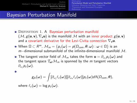
Definition 1. A Bayesian perturbation manifold(M, g(u, v),∇vu) is the manifold M with an inner product g(u, v)and a covariant derivative for the Levi-Civita connection ∇vu.
When Ω ⊂ Rm, Mm = pc(ω) = p(Dcom,θ;ω) : ω ∈ Ω is anm−dimensional submanifold of the infinite-dimensional manifold M.
The tangent vector field of Mm takes the form u = ∂ωj pc(ω) andthe tangent space TωMm is spanned by the m tangent vectors∂ωj pc(ω).
gjk(ω) =
∫[∂ωj `c(ω)][∂ωk
`c(ω)]pc(ω)dΛ(Dcom,θ),
where `c(ω) = log pc(ω).
55 / 98
OutlineMethod I: Perturbation and Scaled Cook’s Distance
Method II: Sensitivity AnalysisAcknowledgement
MotivationPerturbation Model and Perturbation ManifoldInfluence Measures and their PropertiesTheoretical and Simulated ExamplesReferences
Bayesian Perturbation Manifold
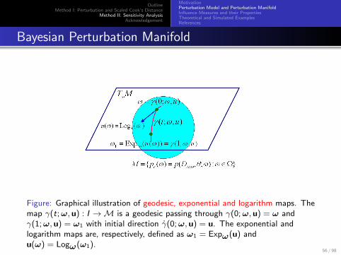
Figure: Graphical illustration of geodesic, exponential and logarithm maps. Themap γ(t;ω, u) : I →M is a geodesic passing through γ(0;ω, u) = ω andγ(1;ω, u) = ω1 with initial direction γ(0;ω, u) = u. The exponential andlogarithm maps are, respectively, defined as ω1 = Expω(u) andu(ω) = Logω(ω1).
56 / 98
OutlineMethod I: Perturbation and Scaled Cook’s Distance
Method II: Sensitivity AnalysisAcknowledgement
MotivationPerturbation Model and Perturbation ManifoldInfluence Measures and their PropertiesTheoretical and Simulated ExamplesReferences
Bayesian Perturbation Manifold
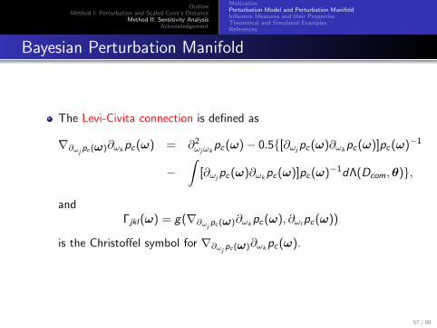
The Levi-Civita connection is defined as
∇∂ωjpc (ω)∂ωk
pc(ω) = ∂2ωjωk
pc(ω)− 0.5[∂ωj pc(ω)∂ωkpc(ω)]pc(ω)−1
−∫
[∂ωj pc(ω)∂ωkpc(ω)]pc(ω)−1dΛ(Dcom,θ),
andΓjkl(ω) = g(∇∂ωj
pc (ω)∂ωkpc(ω), ∂ωl
pc(ω))
is the Christoffel symbol for ∇∂ωjpc (ω)∂ωk
pc(ω).
57 / 98

OutlineMethod I: Perturbation and Scaled Cook’s Distance
Method II: Sensitivity AnalysisAcknowledgement
MotivationPerturbation Model and Perturbation ManifoldInfluence Measures and their PropertiesTheoretical and Simulated ExamplesReferences
Examples of Bayesian Perturbation Manifolds
BPM for the Prior
For the parametric family perturbation to the prior,
gjk(ωP) =
∫[∂ωj `(θ;ωP)∂ωk
`(θ;ωP)]p(θ;ωP)dΛ(θ), (13)
where `(θ;ωP) = log p(θ;ωP).
We consider a hierarchical structure for the prior,
p(θ) = p(θ1)p(θ2;θ[1]) · · · p(θp;θ[p−1])
and
p(θ;ωP) = p(θ1;ωP,1)p(θ2; θ[1], ωP,2) · · · p(θp; θ[p−1], ωP,p), (14)
where θ[j] = (θ1, · · · , θj−1).
58 / 98

OutlineMethod I: Perturbation and Scaled Cook’s Distance
Method II: Sensitivity AnalysisAcknowledgement
MotivationPerturbation Model and Perturbation ManifoldInfluence Measures and their PropertiesTheoretical and Simulated ExamplesReferences
Bayesian Perturbation Manifold
Different ωP,j are orthogonal to each other, that is gjk(ω) = 0 for allj 6= k .
All geometric quantities (e.g., geodesic) of the BPM for the prior areindependent of the sampling distribution.
59 / 98

OutlineMethod I: Perturbation and Scaled Cook’s Distance
Method II: Sensitivity AnalysisAcknowledgement
MotivationPerturbation Model and Perturbation ManifoldInfluence Measures and their PropertiesTheoretical and Simulated ExamplesReferences
Examples of Bayesian Perturbation Manifolds
BPM for the ε−contamination class of priors
This BPM is an infinite dimensional manifold. Recall that
ωP(θ) = ε[g(θ)− p(θ)].
We substitute ε with t in ωP(θ), which yields
ωP(θ) = ωP(t, g(θ)) = t[g(θ)− p(θ)].
Considering
vj(ω0P) = ωP(t, gj(θ)) = [gj(θ)− p(θ)]p(Dcom;θ)
for j = 1, 2, we get
g(v1, v2)(ω0P) =
∫[g1(θ)/p(θ)− 1][g2(θ)/p(θ)− 1]p(θ)dΛ(θ),
which is independent of p(Dcom;θ).
60 / 98

OutlineMethod I: Perturbation and Scaled Cook’s Distance
Method II: Sensitivity AnalysisAcknowledgement
MotivationPerturbation Model and Perturbation ManifoldInfluence Measures and their PropertiesTheoretical and Simulated ExamplesReferences
Examples of Bayesian Perturbation Manifolds
g(v, v)(ω0P) =
∫[g(θ)/p(θ)− 1]2p(θ)dΛ(θ)
reduces to the L2 norm considered in Gustafson (1996a).
The BPMs for all perturbations to the prior are independent of thespecification of the sampling distribution.
61 / 98

OutlineMethod I: Perturbation and Scaled Cook’s Distance
Method II: Sensitivity AnalysisAcknowledgement
MotivationPerturbation Model and Perturbation ManifoldInfluence Measures and their PropertiesTheoretical and Simulated ExamplesReferences
Examples of Bayesian Perturbation Manifolds
BPM for the single-case perturbation scheme to the sampling distribution
For the independent-type-incomplete-data model, the complete-datadensity for the single-case perturbation may be defined by
p(Dcom;θ,ωS) =n∏
i=1
p(di,c ;θ, ωS,i ),
This BPM is a finite dimensional manifold with metric tensor
gjk(ωS) =
∫gjk(θ;ωS)p(θ)dΛ(θ)
for j , k = 1, · · · , n, where
gjk(θ;ωS) = δjk
∫[∂ωS,j
log p(dj,c , ωS,j ;θ)]⊗2p(dj,c ;θ)dΛ(Dcom).
If p(θ) concentrates on θmle , then we obtain the metric tensorgjk(ωS) = gjk(θmle ;ωS) defined in Zhu et al. (2007).
62 / 98
OutlineMethod I: Perturbation and Scaled Cook’s Distance
Method II: Sensitivity AnalysisAcknowledgement
MotivationPerturbation Model and Perturbation ManifoldInfluence Measures and their PropertiesTheoretical and Simulated ExamplesReferences
Bayesian Perturbation Manifold
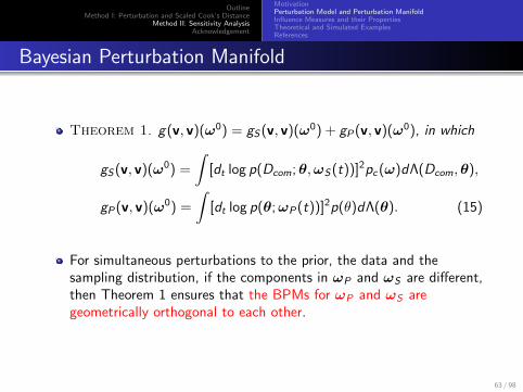
Theorem 1. g(v, v)(ω0) = gS(v, v)(ω0) + gP(v, v)(ω0), in which
gS(v, v)(ω0) =
∫[dt log p(Dcom;θ,ωS(t))]2pc(ω)dΛ(Dcom,θ),
gP(v, v)(ω0) =
∫[dt log p(θ;ωP(t))]2p(θ)dΛ(θ). (15)
For simultaneous perturbations to the prior, the data and thesampling distribution, if the components in ωP and ωS are different,then Theorem 1 ensures that the BPMs for ωP and ωS aregeometrically orthogonal to each other.
63 / 98

OutlineMethod I: Perturbation and Scaled Cook’s Distance
Method II: Sensitivity AnalysisAcknowledgement
MotivationPerturbation Model and Perturbation ManifoldInfluence Measures and their PropertiesTheoretical and Simulated ExamplesReferences
Global Influence Measures
We develop several global influence measures for quantifying the effectsof perturbing the three key elements of a Bayesian analysis.
Let pc(ω0) and pc(ω) represent the unperturbed and perturbedcomplete-data distributions.
Let C (t) = pc(ω(t)) : [−δ, δ]→M be a smooth curve on Mjoining pc(ω0) and pc(ω(s)) such that C (0) = pc(ω0) andC (1) = pc(ω), where δ > 1.
We consider a smooth function of interest
f (ω) = f (pc(ω)) :M→ R
for sensitivity analysis. Thus,
f (ω(t)) : [−δ, δ]→ R
is a real function of t.
64 / 98
OutlineMethod I: Perturbation and Scaled Cook’s Distance
Method II: Sensitivity AnalysisAcknowledgement
MotivationPerturbation Model and Perturbation ManifoldInfluence Measures and their PropertiesTheoretical and Simulated ExamplesReferences
Global Influence Measures
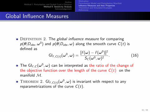
Definition 2. The global influence measure for comparingp(θ|Dobs ,ω
0) and p(θ|Dobs ,ω) along the smooth curve C (t) isdefined as
GIf ,C(t)(ω0,ω) =
[f (ω)− f (ω0)]2
SC (ω0,ω)2. (16)
The GIf ,C (ω0,ω) can be interpreted as the ratio of the change ofthe objective function over the length of the curve C (t) on themanifold M.
Theorem 2. GIf ,C(t)(ω0,ω) is invariant with respect to any
reparametrizations of the curve C (t).
65 / 98
OutlineMethod I: Perturbation and Scaled Cook’s Distance
Method II: Sensitivity AnalysisAcknowledgement
MotivationPerturbation Model and Perturbation ManifoldInfluence Measures and their PropertiesTheoretical and Simulated ExamplesReferences
Global Influence Measures
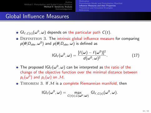
GIf ,C(t)(ω0,ω) depends on the particular path C (t).
Definition 3. The intrinsic global influence measure for comparingp(θ|Dobs ,ω
0) and p(θ|Dobs ,ω) is defined as
IGIf (ω0,ω) =[f (ω)− f (ω0)]2
d(ω0,ω)2. (17)
The proposed IGIf (ω0,ω) can be interpreted as the ratio of thechange of the objective function over the minimal distance betweenpc(ω0) and pc(ω) on M.
Theorem 3. If M is a complete Riemannian manifold, then
IGIf (ω0,ω) = maxC(t)∈L(ω0,ω)
GIf ,C(t)(ω0,ω).
66 / 98
OutlineMethod I: Perturbation and Scaled Cook’s Distance
Method II: Sensitivity AnalysisAcknowledgement
MotivationPerturbation Model and Perturbation ManifoldInfluence Measures and their PropertiesTheoretical and Simulated ExamplesReferences
Global Influence Measures
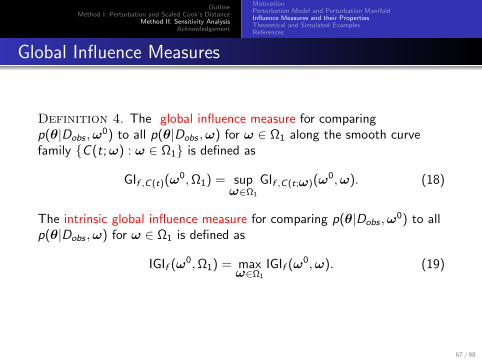
Definition 4. The global influence measure for comparingp(θ|Dobs ,ω
0) to all p(θ|Dobs ,ω) for ω ∈ Ω1 along the smooth curvefamily C (t;ω) : ω ∈ Ω1 is defined as
GIf ,C(t)(ω0,Ω1) = sup
ω∈Ω1
GIf ,C(t;ω)(ω0,ω). (18)
The intrinsic global influence measure for comparing p(θ|Dobs ,ω0) to all
p(θ|Dobs ,ω) for ω ∈ Ω1 is defined as
IGIf (ω0,Ω1) = maxω∈Ω1
IGIf (ω0,ω). (19)
67 / 98

OutlineMethod I: Perturbation and Scaled Cook’s Distance
Method II: Sensitivity AnalysisAcknowledgement
MotivationPerturbation Model and Perturbation ManifoldInfluence Measures and their PropertiesTheoretical and Simulated ExamplesReferences
Local Influence Measures
f (ω(t)) = f (ω(0)) + f (ω(0))t + 0.5f (ω(0))t2 + o(t2).
We need to distinguish two cases: f (ω(0)) 6= 0 for some smoothcurves ω(t) and f (ω(0)) = 0 for all smooth curves ω(t). Iff (ω(0)) = 0 for all smooth curves ω(t), then we have to considerthe second order term f (ω(0)) in order to characterize the localbehavior of f (ω(t)).
Definition 5. The first-order local influence measure is defined as
FIf [v](ω(0)) = limt→0
GIf ,C(t)(ω(0),ω(t)) =[df [v](ω(0))]2
g(v, v)(ω(0)). (20)
68 / 98
OutlineMethod I: Perturbation and Scaled Cook’s Distance
Method II: Sensitivity AnalysisAcknowledgement
MotivationPerturbation Model and Perturbation ManifoldInfluence Measures and their PropertiesTheoretical and Simulated ExamplesReferences
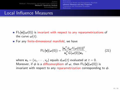
Local Influence Measures
FIf [v](ω(0)) is invariant with respect to any reparametrizations ofthe curve ω(t).
For any finite-dimensional manifold, we have
FIf [v](ω(0)) =[vT
h ∂ωf (ω(0))]2
vTh G (ω(0))vh
, (21)
where vh = (v1, · · · , vp) equals dtω(t) evaluated at t = 0.Moreover, if φ is a diffeomorphism of ω, then FIf [v](ω(0)) isinvariant with respect to any reparametrization corresponding to φ.
69 / 98
OutlineMethod I: Perturbation and Scaled Cook’s Distance
Method II: Sensitivity AnalysisAcknowledgement
MotivationPerturbation Model and Perturbation ManifoldInfluence Measures and their PropertiesTheoretical and Simulated ExamplesReferences
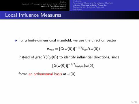
Local Influence Measures
For a finite-dimensional manifold, we use the direction vector
vmax = [G (ω(0))]−1/2∂ωf (ω(0))
instead of grad(f )(ω(0)) to identify influential directions, since
[G (ω(0))]−1/2∂ωpc(ω(0))
forms an orthonormal basis at ω(0).
70 / 98
OutlineMethod I: Perturbation and Scaled Cook’s Distance
Method II: Sensitivity AnalysisAcknowledgement
MotivationPerturbation Model and Perturbation ManifoldInfluence Measures and their PropertiesTheoretical and Simulated ExamplesReferences
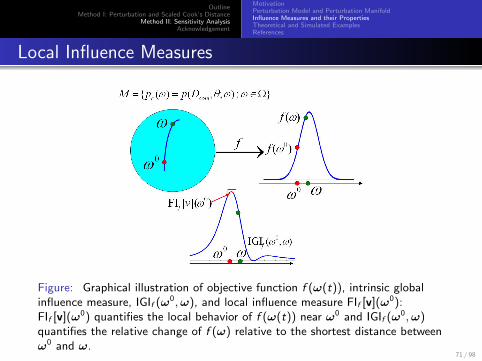
Local Influence Measures
Figure: Graphical illustration of objective function f (ω(t)), intrinsic globalinfluence measure, IGIf (ω0,ω), and local influence measure FIf [v](ω0):FIf [v](ω0) quantifies the local behavior of f (ω(t)) near ω0 and IGIf (ω0,ω)quantifies the relative change of f (ω) relative to the shortest distance betweenω0 and ω.
71 / 98

OutlineMethod I: Perturbation and Scaled Cook’s Distance
Method II: Sensitivity AnalysisAcknowledgement
MotivationPerturbation Model and Perturbation ManifoldInfluence Measures and their PropertiesTheoretical and Simulated ExamplesReferences
Local Influence Measures
We only consider the geodesic pc(ω(t)) = Exppc (ω(0))(tv) that
satisfies pc(ω(0)) = pc(ω0) and dtpc(ω(0)) = v ∈ Tω(0)M.
We obtain a covariant version of Taylor’s theorem as follows:
f (Expω(0)(tv)) = f (ω0) + tdf [v](ω(0)) + 0.5t2Hess(f )(v, v)(ω(0)) + o(t2),
where Hess(f )(v, v)(ω(0)) = f (Expω(0)(tv))|t=0 is a covariant (orRiemmanian) Hessian.
Geometrically, Hess(f )(u, v)(ω(0)) is a tensor of type (0,2) anddefined as
Hess(f )(u, v)(ω(0)) = d(df [v])[u](ω(0))− df [∇uv](ω(0)). (22)
72 / 98
OutlineMethod I: Perturbation and Scaled Cook’s Distance
Method II: Sensitivity AnalysisAcknowledgement
MotivationPerturbation Model and Perturbation ManifoldInfluence Measures and their PropertiesTheoretical and Simulated ExamplesReferences
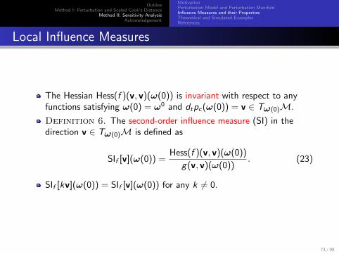
Local Influence Measures
The Hessian Hess(f )(v, v)(ω(0)) is invariant with respect to anyfunctions satisfying ω(0) = ω0 and dtpc(ω(0)) = v ∈ Tω(0)M.
Definition 6. The second-order influence measure (SI) in thedirection v ∈ Tω(0)M is defined as
SIf [v](ω(0)) =Hess(f )(v, v)(ω(0))
g(v, v)(ω(0)). (23)
SIf [kv](ω(0)) = SIf [v](ω(0)) for any k 6= 0.
73 / 98
OutlineMethod I: Perturbation and Scaled Cook’s Distance
Method II: Sensitivity AnalysisAcknowledgement
MotivationPerturbation Model and Perturbation ManifoldInfluence Measures and their PropertiesTheoretical and Simulated ExamplesReferences
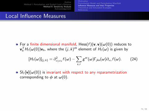
Local Influence Measures
For a finite dimensional manifold, Hess(f )(v, v)(ω(0)) reduces tovTh Hf (ω(0))vh, where the (j , k)th element of Hf (ω) is given by
[Hf (ω)](j,k) = ∂2ωjωk
f (ω)−∑s,r
g sr (ω)Γjks(ω)∂ωr f (ω). (24)
SIf [v](ω(0)) is invariant with respect to any reparametrizationcorresponding to φ at ω(0).
74 / 98

OutlineMethod I: Perturbation and Scaled Cook’s Distance
Method II: Sensitivity AnalysisAcknowledgement
MotivationPerturbation Model and Perturbation ManifoldInfluence Measures and their PropertiesTheoretical and Simulated ExamplesReferences
Theoretical Examples
Bayes Factor
f (ω) = B(ω) and ω(t) is a smooth curve on M with ω(0) = ω0
and dtpc(ω(t))|t=0 = v ∈ Tω(0)M.
B(ω) = log p(Dobs ;ω)− log p(Dobs ;ω0)
is a continuous map from M to R.
We consider the simultaneous perturbation to both the prior and thesampling distribution and, therefore we have
FIB [v](ω(0)) =E [dt log p(Dcom,θ;ω(t))|Dobs ]2
gP(v, v) + gS(v, v). (25)
75 / 98

OutlineMethod I: Perturbation and Scaled Cook’s Distance
Method II: Sensitivity AnalysisAcknowledgement
MotivationPerturbation Model and Perturbation ManifoldInfluence Measures and their PropertiesTheoretical and Simulated ExamplesReferences
Theoretical Examples
For p(θ; t) = p(θ) + t[g(θ)− p(θ)], we have
FIB [v](ω(0))] =E[g(θ)/p(θ)|Dobs ]2
VarP(g(θ)/p(θ))=
[pg (Dobs)/p(Dobs)]2
VarP(g(θ)/p(θ)), (26)
where
p(Dobs) =
∫p(Dcom;θ)p(θ)dΛ(Dmis ,θ)
and
pg (Dobs) =
∫p(Dcom;θ)g(θ)dΛ(Dmis ,θ).
FIB [v](ω(0))] is the square of the normalized Bayes factor of g(θ)against p(θ).
76 / 98

OutlineMethod I: Perturbation and Scaled Cook’s Distance
Method II: Sensitivity AnalysisAcknowledgement
MotivationPerturbation Model and Perturbation ManifoldInfluence Measures and their PropertiesTheoretical and Simulated ExamplesReferences
Theoretical Examples
Bayes Factor
For a perturbation scheme to the sampling distribution,
f (ω(0)) = E [dt`c(θ,ω(0))|Dobs ] ≈ dt`o(θ,ω(0))
and
FIB [v](ω(0))] =E [dt`c(θ,ω(0))|Dobs ]2
gS(v, v)≈ [dt`o(θ,ω(0))]2
gS(v, v),
where`o(θ,ω(t)) = log p(Dobs ; θ,ω(t))
and`c(θ,ω(t)) = log p(Dcom; θ,ω(t)).
77 / 98
OutlineMethod I: Perturbation and Scaled Cook’s Distance
Method II: Sensitivity AnalysisAcknowledgement
MotivationPerturbation Model and Perturbation ManifoldInfluence Measures and their PropertiesTheoretical and Simulated ExamplesReferences
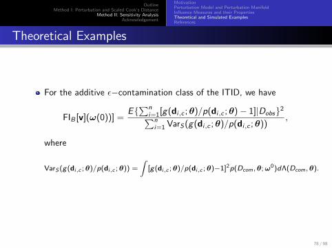
Theoretical Examples
For the additive ε−contamination class of the ITID, we have
FIB [v](ω(0))] =E∑n
i=1[g(di,c ;θ)/p(di,c ;θ)− 1]|Dobs2∑ni=1 VarS(g(di,c ;θ)/p(di,c ;θ))
,
where
VarS (g(di,c ;θ)/p(di,c ;θ)) =
∫[g(di,c ;θ)/p(di,c ;θ)−1]2p(Dcom,θ;ω0)dΛ(Dcom,θ).
78 / 98
OutlineMethod I: Perturbation and Scaled Cook’s Distance
Method II: Sensitivity AnalysisAcknowledgement
MotivationPerturbation Model and Perturbation ManifoldInfluence Measures and their PropertiesTheoretical and Simulated ExamplesReferences
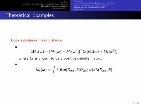
Theoretical Examples
Cook’s posterior mean distance
CMh(ω) = [Mh(ω)−Mh(ω0)]TCh[Mh(ω)−Mh(ω0)],
where Ch is chosen to be a positive definite matrix.
Mh(ω) =
∫h(θ)p(Dmis ,θ|Dobs ;ω)dΛ(Dmis ,θ).
79 / 98

OutlineMethod I: Perturbation and Scaled Cook’s Distance
Method II: Sensitivity AnalysisAcknowledgement
MotivationPerturbation Model and Perturbation ManifoldInfluence Measures and their PropertiesTheoretical and Simulated ExamplesReferences
Theoretical Examples
We set f (ω) = CMh(ω) and ω(t) is a smooth curve on M withω(0) = ω0 and
dtpc(ω(0)) = v ∈ Tω(0)M.
f (ω(0)) = 0 and
f (ω(0)) = Mh(v)TGhMh(v),
where
Mh(v) = Covh(θ), dt log p(Dcom,θ;ω(t))|Dobs|t=0. (27)
80 / 98

OutlineMethod I: Perturbation and Scaled Cook’s Distance
Method II: Sensitivity AnalysisAcknowledgement
MotivationPerturbation Model and Perturbation ManifoldInfluence Measures and their PropertiesTheoretical and Simulated ExamplesReferences
Theoretical Examples
We consider a simultaneous perturbation to both the prior and thesampling distribution.
SICMh[v](ω(0)) = Mh(v)TGhMh(v)
gP (v,v)+gS (v,v) .
For the perturbation to the prior,
p(θ; t) = p(θ) + t[g(θ)− p(θ)],
and SICMh[v](ω(0)) is given by
Covg(θ)/p(θ), h(θ)T |DobsChCovh(θ), g(θ)/p(θ)|DobsVarP(g(θ)/p(θ))
.
81 / 98
OutlineMethod I: Perturbation and Scaled Cook’s Distance
Method II: Sensitivity AnalysisAcknowledgement
MotivationPerturbation Model and Perturbation ManifoldInfluence Measures and their PropertiesTheoretical and Simulated ExamplesReferences
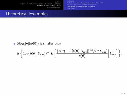
Theoretical Examples
SICMh[v](ω(0)) is smaller than
tr
Covh(θ)|Dobs)−1E
[h(θ)− E [h(θ)|Dobs ]⊗2p(θ|Dobs)
p(θ)
∣∣∣∣Dobs
].
82 / 98
OutlineMethod I: Perturbation and Scaled Cook’s Distance
Method II: Sensitivity AnalysisAcknowledgement
MotivationPerturbation Model and Perturbation ManifoldInfluence Measures and their PropertiesTheoretical and Simulated ExamplesReferences
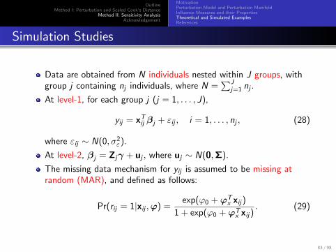
Simulation Studies
Data are obtained from N individuals nested within J groups, withgroup j containing nj individuals, where N =
∑Jj=1 nj .
At level-1, for each group j (j = 1, . . . , J),
yij = xTij βj + εij , i = 1, . . . , nj , (28)
where εij ∼ N(0, σ2ε).
At level-2, βj = Zjγ + uj , where uj ∼ N(0,Σ).
The missing data mechanism for yij is assumed to be missing atrandom (MAR), and defined as follows:
Pr(rij = 1|xij ,ϕ) =exp(ϕ0 +ϕT
x xij)
1 + exp(ϕ0 +ϕTx xij)
. (29)
83 / 98
OutlineMethod I: Perturbation and Scaled Cook’s Distance
Method II: Sensitivity AnalysisAcknowledgement
MotivationPerturbation Model and Perturbation ManifoldInfluence Measures and their PropertiesTheoretical and Simulated ExamplesReferences
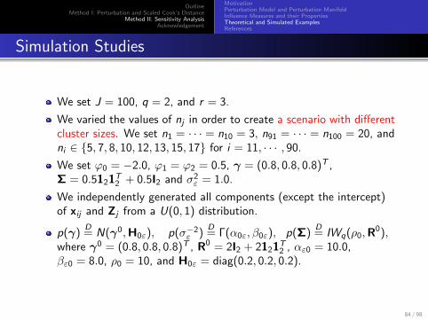
Simulation Studies
We set J = 100, q = 2, and r = 3.
We varied the values of nj in order to create a scenario with differentcluster sizes. We set n1 = · · · = n10 = 3, n91 = · · · = n100 = 20, andni ∈ 5, 7, 8, 10, 12, 13, 15, 17 for i = 11, · · · , 90.
We set ϕ0 = −2.0, ϕ1 = ϕ2 = 0.5, γ = (0.8, 0.8, 0.8)T ,Σ = 0.5121T
2 + 0.5I2 and σ2ε = 1.0.
We independently generated all components (except the intercept)of xij and Zj from a U(0, 1) distribution.
p(γ)D= N(γ0,H0ε), p(σ−2
ε )D= Γ(α0ε, β0ε), p(Σ)
D= IWq(ρ0,R
0),where γ0 = (0.8, 0.8, 0.8)T , R0 = 2I2 + 2121T
2 , αε0 = 10.0,βε0 = 8.0, ρ0 = 10, and H0ε = diag(0.2, 0.2, 0.2).
84 / 98
OutlineMethod I: Perturbation and Scaled Cook’s Distance
Method II: Sensitivity AnalysisAcknowledgement
MotivationPerturbation Model and Perturbation ManifoldInfluence Measures and their PropertiesTheoretical and Simulated ExamplesReferences
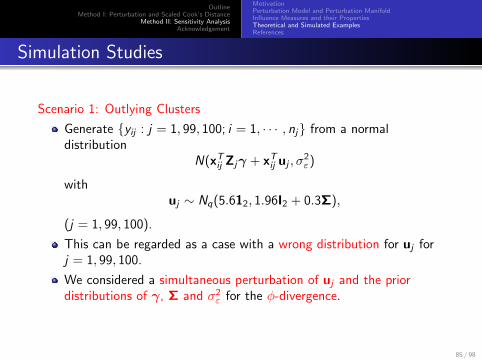
Simulation Studies
Scenario 1: Outlying Clusters
Generate yij : j = 1, 99, 100; i = 1, · · · , nj from a normaldistribution
N(xTij Zjγ + xTij uj , σ2ε)
withuj ∼ Nq(5.612, 1.96I2 + 0.3Σ),
(j = 1, 99, 100).
This can be regarded as a case with a wrong distribution for uj forj = 1, 99, 100.
We considered a simultaneous perturbation of uj and the priordistributions of γ, Σ and σ2
ε for the φ-divergence.
85 / 98
OutlineMethod I: Perturbation and Scaled Cook’s Distance
Method II: Sensitivity AnalysisAcknowledgement
MotivationPerturbation Model and Perturbation ManifoldInfluence Measures and their PropertiesTheoretical and Simulated ExamplesReferences
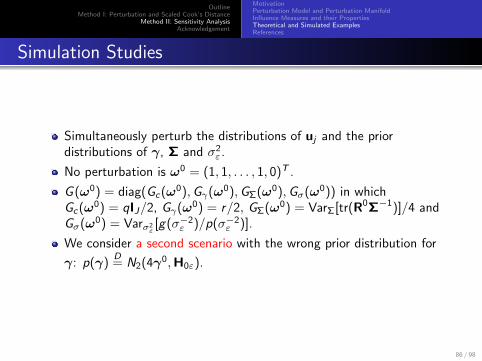
Simulation Studies
Simultaneously perturb the distributions of uj and the priordistributions of γ, Σ and σ2
ε.
No perturbation is ω0 = (1, 1, . . . , 1, 0)T .
G (ω0) = diag(Gc(ω0),Gγ(ω0),GΣ(ω0),Gσ(ω0)) in whichGc(ω0) = qIJ/2, Gγ(ω0) = r/2, GΣ(ω0) = VarΣ[tr(R0Σ−1)]/4 andGσ(ω0) = Varσ2
ε[g(σ−2
ε )/p(σ−2ε )].
We consider a second scenario with the wrong prior distribution for
γ: p(γ)D= N2(4γ0,H0ε).
86 / 98
OutlineMethod I: Perturbation and Scaled Cook’s Distance
Method II: Sensitivity AnalysisAcknowledgement
MotivationPerturbation Model and Perturbation ManifoldInfluence Measures and their PropertiesTheoretical and Simulated ExamplesReferences
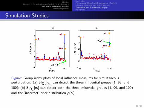
Simulation Studies
Figure: Group index plots of local influence measures for simultaneousperturbation: (a) SIDφ
[ej ] can detect the three influential groups (1, 99, and
100); (b) SIDφ[ej ] can detect both the three influential groups (1, 99, and 100)
and the ’incorrect’ prior distribution p(γ).
87 / 98

OutlineMethod I: Perturbation and Scaled Cook’s Distance
Method II: Sensitivity AnalysisAcknowledgement
MotivationPerturbation Model and Perturbation ManifoldInfluence Measures and their PropertiesTheoretical and Simulated ExamplesReferences
Simulation Studies
Scenario 2: Missing-data Mechanism
Explore the potential deviations of the MAR missing datamechanism in the direction of nonignorable MAR (NMAR).
We simulated a data set using the same setup as above except thatthe following missing data mechanism for yij was assumed,
Pr(rij = 1|xij , yij ,ϕ, ϕy ) =exp(ϕ0 +ϕ′xxij + ϕyyij)
1 + exp(ϕ0 +ϕ′xxij + ϕyyij)(30)
with ϕy = 0.5 to make the missing data fraction approximately 25%.
When ϕy 6= 0, the missing mechanism is nonignorable.
88 / 98
OutlineMethod I: Perturbation and Scaled Cook’s Distance
Method II: Sensitivity AnalysisAcknowledgement
MotivationPerturbation Model and Perturbation ManifoldInfluence Measures and their PropertiesTheoretical and Simulated ExamplesReferences
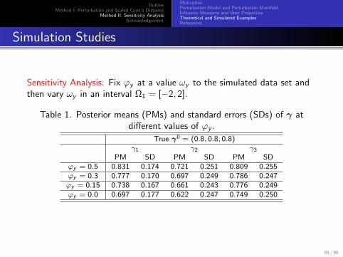
Simulation Studies
Sensitivity Analysis: Fix ϕy at a value ωy to the simulated data set andthen vary ωy in an interval Ω1 = [−2, 2].
Table 1. Posterior means (PMs) and standard errors (SDs) of γ atdifferent values of ϕy .
True γ0 = (0.8, 0.8, 0.8)γ1 γ2 γ3
PM SD PM SD PM SDϕy = 0.5 0.831 0.174 0.721 0.251 0.809 0.255ϕy = 0.3 0.777 0.170 0.697 0.249 0.786 0.247ϕy = 0.15 0.738 0.167 0.661 0.243 0.776 0.249ϕy = 0.0 0.697 0.177 0.622 0.247 0.749 0.250
89 / 98
OutlineMethod I: Perturbation and Scaled Cook’s Distance
Method II: Sensitivity AnalysisAcknowledgement
MotivationPerturbation Model and Perturbation ManifoldInfluence Measures and their PropertiesTheoretical and Simulated ExamplesReferences
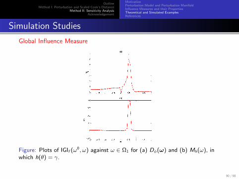
Simulation Studies
Global Influence Measure
Figure: Plots of IGIf (ω0, ω) against ω ∈ Ω1 for (a) Dφ(ω) and (b) Mh(ω), inwhich h(θ) = γ.
90 / 98
OutlineMethod I: Perturbation and Scaled Cook’s Distance
Method II: Sensitivity AnalysisAcknowledgement
MotivationPerturbation Model and Perturbation ManifoldInfluence Measures and their PropertiesTheoretical and Simulated ExamplesReferences
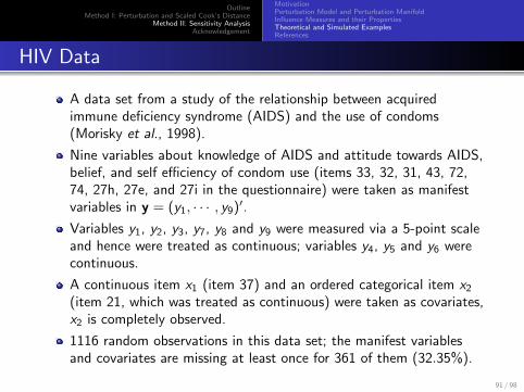
HIV Data
A data set from a study of the relationship between acquiredimmune deficiency syndrome (AIDS) and the use of condoms(Morisky et al., 1998).
Nine variables about knowledge of AIDS and attitude towards AIDS,belief, and self efficiency of condom use (items 33, 32, 31, 43, 72,74, 27h, 27e, and 27i in the questionnaire) were taken as manifestvariables in y = (y1, · · · , y9)′.
Variables y1, y2, y3, y7, y8 and y9 were measured via a 5-point scaleand hence were treated as continuous; variables y4, y5 and y6 werecontinuous.
A continuous item x1 (item 37) and an ordered categorical item x2
(item 21, which was treated as continuous) were taken as covariates,x2 is completely observed.
1116 random observations in this data set; the manifest variablesand covariates are missing at least once for 361 of them (32.35%).
91 / 98
OutlineMethod I: Perturbation and Scaled Cook’s Distance
Method II: Sensitivity AnalysisAcknowledgement
MotivationPerturbation Model and Perturbation ManifoldInfluence Measures and their PropertiesTheoretical and Simulated ExamplesReferences
HIV Data
yi = µ+ Λ$i + εi , i = 1, · · · , 1116, in which yi = (yi1, · · · , yi9)′
and $i = (ηi , ξi1, ξi2)′ via the following specifications ofµ = (µ1, · · · , µ9)′ and
Λ′ =
(1.0∗ λ21 λ31 0.0∗ 0.0∗ 0.0∗ 0.0∗ 0.0∗ 0.0∗
0.0∗ 0.0∗ 0.0∗ 1.0∗ λ52 λ62 0.0∗ 0.0∗ 0.0∗
0.0∗ 0.0∗ 0.0∗ 0.0∗ 0.0∗ 0.0∗ 1.0∗ λ83 λ93
),
and εi ∼ N(0,Ψ) distribution for i = 1, · · · , 9.
η=‘threat of AIDS’, ξ1 =‘aggressiveness of the sex worker’, andξ2=‘worry of contracting AIDS’.
ηi = b1xi1 + b2xi2 + γ1ξi1 + γ2ξi2 + δi , where δi ∼ N(0, ψδ),
logitPr(ryij = 1|ϕ) = ϕ0 + ϕ1yi1 + · · ·+ ϕ9yi9, whereϕ = (ϕ0, ϕ1, · · · , ϕ9)′.
logitPr(rxi1 = 1|ϕx) = ϕx0 + ωxi1.
92 / 98
OutlineMethod I: Perturbation and Scaled Cook’s Distance
Method II: Sensitivity AnalysisAcknowledgement
MotivationPerturbation Model and Perturbation ManifoldInfluence Measures and their PropertiesTheoretical and Simulated ExamplesReferences
HIV Data
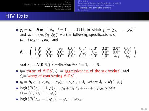
Global influence measures for the Kullback-Leibler divergence and Mh(ω)
Figure: HIV data: IGIf (ω0, ω) against ω ∈ [−2, 2] for (a) the Kullback-Leiblerdivergence and (b) Mh(ω), in which h(θ) = Γ = (b1, b2, γ1, γ2)T .
93 / 98
OutlineMethod I: Perturbation and Scaled Cook’s Distance
Method II: Sensitivity AnalysisAcknowledgement
MotivationPerturbation Model and Perturbation ManifoldInfluence Measures and their PropertiesTheoretical and Simulated ExamplesReferences
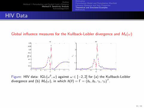
HIV Data
Sensitivity analysis
Figure: HIV data: the posterior means (red solid lines and dots) andmeans±2×SD (blue lines and dots) of b1 (a), b2 (b), γ1 (c), and γ2 (d) againstω ∈ [−2, 2], where SD denotes standard deviation.
94 / 98

OutlineMethod I: Perturbation and Scaled Cook’s Distance
Method II: Sensitivity AnalysisAcknowledgement
MotivationPerturbation Model and Perturbation ManifoldInfluence Measures and their PropertiesTheoretical and Simulated ExamplesReferences
HIV Data
Simultaneous perturbation scheme includes
variance perturbation for individual observationsperturbation to coefficients in the structural equations modelperturbation toηi = b1xi1 + b2xi2 + γ1ξi1 + γ2ξi2 + ωγ,1ξ
2i1 + ωγ,2ξ
2i2 + ωγ,3ξi1ξi2 + δi
perturbation to the prior distribution of µperturbation to the prior distribution of Γperturbation to the prior distribution of ϕperturbation to logitPr(rxi1 = 1|ϕx) = ϕx0 + ωxxi1.
We calculated the local influence measures of the Kullback-Leiblerdivergence under a simultaneous perturbation scheme.
95 / 98
OutlineMethod I: Perturbation and Scaled Cook’s Distance
Method II: Sensitivity AnalysisAcknowledgement
MotivationPerturbation Model and Perturbation ManifoldInfluence Measures and their PropertiesTheoretical and Simulated ExamplesReferences
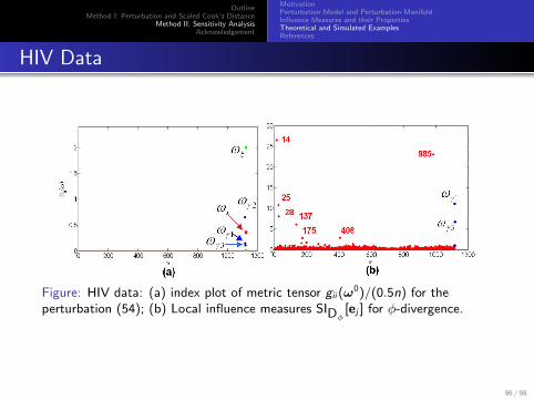
HIV Data
Figure: HIV data: (a) index plot of metric tensor gii (ω0)/(0.5n) for the
perturbation (54); (b) Local influence measures SIDφ[ej ] for φ-divergence.
96 / 98
OutlineMethod I: Perturbation and Scaled Cook’s Distance
Method II: Sensitivity AnalysisAcknowledgement
MotivationPerturbation Model and Perturbation ManifoldInfluence Measures and their PropertiesTheoretical and Simulated ExamplesReferences
References
Zhu, HT., Ibrahim, JG., and Tang, NS. Bayesian influence measures forjoint models for longitudinal and survival data. Biometrics, in press, 2012.
Zhu, HT., Ibrahim JG, Tang NS. Bayesian influence approach: ageometric approach. Biometrika, 98, 307-323, 2011.
Ibrahim, J. G., Zhu, H.T., Tang, N. S. Bayesian local influence for survivalmodels (with discussion). Lifetime Data Analysis, 17, 43-70, 2011.
Zhu HT, Ibrahim, JG, Lee SY, and Zhang HP. Appropriate perturbationand influence measures in local influence. Annals of Statistics, 35,2565-2588, 2007.
Shi, X Y., Zhu HT, Ibrahim, JG. Local influence for generalized linearmodels with missing covariates. Biometrics, 65, 1164-1174, 2009.
Zhu HT and Zhang HP. A diagnostic procedure based on local influence.Biometrika, 91:579-589, 2004.
Zhu HT and Lee SY. Local influence for generalized linear mixed models.Canadian Journal of Statistics, 31:293-309, 2003.
Zhu HT and Lee SY. Local influence for models with incomplete data.Journal of the Royal Statistical Society, Series B, 63:111-126, 2001.
97 / 98

OutlineMethod I: Perturbation and Scaled Cook’s Distance
Method II: Sensitivity AnalysisAcknowledgement
Acknowledgement
Southeast University: Bocheng Wei
University of Minnesota: Dennis Cook
Yale University: Heping Zhang
University of North Carolina at Chapel Hill: Joseph G. Ibrahim
Yunnan University: Niansheng Tang
SAS: Amy Shi
98 / 98
Related Documents