A game theoretic approach to coordinate pricing and vertical co-op advertising in manufacturer-retailer supply chains

European Journal of Operational Research 211 (2011) 263–273

Contents lists available at ScienceDirect

European Journal of Operational Research

journal homepage: www.elsevier .com/locate /e jor

Production, Manufacturing and Logistics

A game theoretic approach to coordinate pricing and vertical co-op advertisingin manufacturer–retailer supply chains

Mir Mehdi SeyedEsfahani a,⇑, Maryam Biazaran a, Mohsen Gharakhani b

a Department of Industrial Engineering, AmirKabir University of Technology, Tehran 15875-4413, Iranb Department of Industrial Engineering, Iran University of Science and Technology, Tehran 16846-13114, Iran

a r t i c l e i n f o

Article history:Received 23 March 2010Accepted 15 November 2010Available online 23 November 2010

Keywords:MarketingSupply chain coordinationPricingVertical cooperative advertisingGame theory

0377-2217/$ - see front matter � 2010 Elsevier B.V. Adoi:10.1016/j.ejor.2010.11.014

⇑ Corresponding author. Tel.: +98 66466497; fax: +E-mail addresses: [email protected] (M.M. Seye

Biazaran), [email protected] (M. Gharakhani).

a b s t r a c t

Vertical cooperative (co-op) advertising is a marketing strategy in which the retailer runs local advertis-ing and the manufacturer pays for a portion of its entire costs. This paper considers vertical co-op adver-tising along with pricing decisions in a supply chain; this consists of one manufacturer and one retailerwhere demand is influenced by both price and advertisement. Four game-theoretic models are estab-lished in order to study the effect of supply chain power balance on the optimal decisions of supply chainmembers. Comparisons and insights are developed. These embrace three non-cooperative games includ-ing Nash, Stackelberg-manufacturer and Stackelberg-retailer, and one cooperative game. In the lattercase, both the manufacturer and the retailer reach the highest profit level; subsequently, the feasibilityof bargaining game is discussed in a bid to determine a scheme to share the extra joint profit.

� 2010 Elsevier B.V. All rights reserved.

1. Introduction

Supply chain coordination has been the focus of many researchstudies without which channel members tend to maximize theirown profit. A prime example associated with such an uncoordi-nated system is ‘‘double marginalization’’, in which the retailermakes arbitrary decisions without considering supplier’s profitmargin (Spengler, 1950). Another example is the ‘‘bullwhip effect’’which occurs when supply chain members make decision ignoringthe others; this, in return, will lead to the spread of distorted de-mand information moving upstream (Lee et al., 1997).

Sahin and Robinson (2002) proposed two key drivers of supplychain performance involving information sharing and coordina-tion. Fugate et al. (2006) classified supply chain coordinationmechanisms into three categories: (1) price coordination, (2)non-price coordination and (3) flow coordination. Based on thisclassification, pricing and vertical cooperative advertising, twobusiness decisions discussed in this paper, are placed in the firstand second category, respectively.

A considerable amount of research has been conducted in re-cent years on different aspects of supply chain coordination includ-ing pricing, production, purchasing, inventory, etc. In this paper,optimal pricing and vertical co-op advertising decision is discussedin a single-manufacturer–single-retailer supply chain in which

ll rights reserved.

98 2188500995.dEsfahani), [email protected] (M.

consumer demand is influenced by both price and advertisingefforts.

Manufacturers and retailers use advertising programs to con-vince customers to purchase their products. Their efforts are differ-ent in the sense that, the aim of manufacturer’s nationaladvertising is to influence potential customers and raise brandawareness, while the Retailer’s local advertising is intended tobring potential customers to the point of desire and action (Huangand Li, 2001). Vertical co-op advertising is an arrangement where-by a manufacturer agrees to pay for a portion or the entire costs oflocal advertising undertaken by a retailer. The percentage of localadvertising cost that the manufacturer agrees to pay is called ‘‘par-ticipation rate’’ (Bergen and John, 1997). The main reason for themanufacturer to use co-op advertising is to strengthen the brandimage and promote immediate sales at the retail level (Hutchins,1953).

The vertical co-op advertising plays an important role in firms’marketing programs. Total expenditures on co-op advertising inthe United States in 2000 were estimated at $15 billion; an approx-imately fourfold increase in real terms compared with $900 millionin 1970 (Nagler, 2006). Berger (1972) was the first to address thevertical co-op advertising problem mathematically. Using a realworld application, he showed the proposed quantitative analysiscan be applied in determining the optimal decisions appropriately.

A common approach in the literature to analyze the role of co-op advertising in supply chain coordination is to use game theoret-ical models; these exist in two categories: static and dynamic. Instatic models, interactions among supply chain members are dis-cussed in a single period. Examples in this category are Dant and

264 M.M. SeyedEsfahani et al. / European Journal of Operational Research 211 (2011) 263–273

Berger (1996), Bergen and John (1997), Kim and Staelin (1999),Karray and Zaccour (2006, 2007), Huang and Li (2001), Huanget al. (2002) and Li et al. (2002). In dynamic models, a goodwillfunction is introduced to express the carry-over effect of advertis-ing. Most of the studies in this category ignore the participationrate despite its fundamental role. Reader is referred to Jørgensenet al. (2001, 2000) and Jørgensen and Zaccour (2003b) for moreexamples. On the other hand, when the retailer has perfect knowl-edge about manufacturer’s decision in advertising policy or in thecase it has already been announced, the required assumptions ofgame-theoretic model do not hold. Berger et al. (2006) consideredsuch issue in co-op advertising problem. Determining retail/whole-sale price has been the focus of many studies, as a fundamentaltask in the supply chain management literature. Jeuland andShugan (1983, 1988), McGuire and Staelin (1983), Moorthy(1988), Ingene and Parry (1995a,b, 1998, 2000) and Choi (1991,1996) discuss channel coordination in the context of two-levelsupply chain; they do this by adopting two common pricing mech-anisms as well as two-part tariffs and quantity discounts. There area number of studies that consider pricing and advertising decisionssimultaneously in supply chain coordination. Jørgensen andZaccour (1999) proposed a differential game model in which theyconsider pricing and advertising decisions in a two-level supplychain under channel conflict and coordination. In their study, con-sumer demand is influenced by retail price and advertising good-will. Jørgensen et al. (2001), considered the leadership role in asingle-manufacturer–single-retailer marketing channel; eachplayer controls her advertising and margin. In their model, con-sumer demand is influenced by both advertising goodwill and re-tail price. They proposed four game-theoretic models andcompared the results. Jørgensen and Zaccour (2003a) also modeledconsumer demand as the multiplicative product of retail price andadvertising goodwill in dynamic setting, and then compared re-sults in coordinated strategies with all those of uncoordinated.

In the static framework, Yue et al. (2006) extended the model ofHuang et al. (2002); they did this by considering a price-sensitivedemand and studied the impact direct discount from manufacturerto the costumer may have on the channel coordination. In his paper,Zaccour (2008) attempted to study the conditions that may lead themanufacturer to achieve the integrate channel solution by means ofa two-part tariff wholesale price. He further compared static anddynamic models in which demand function is affected by priceand advertising. He et al. (2009) modeled a single-manufacturer–single-retailer supply chain as a stochastic Stackelberg differentialgame; in this game the demand is a function of both retailer’s priceand advertising. Szmerekovsky and Zhang (2009) considered pric-ing and advertising in a two-member supply chain; where cos-tumer demand depends on both retail price and advertisement.They obtained both the manufacturer and the retailer’s optimaldecisions by solving the Stackelberg-manufacturer. Xie and Neyret(2009) and Xie and Wei (2009) followed a similar approach; theycompared the cooperative game optimal results with those ofnon-cooperative. Xie and Neyret (2009) investigated four game

Table 1Comparing the current paper with three most related studies.

Demand function Szmerekovsky and Zhang (2009) Xie and Neyret

Price effect p�e (e > 1) a1 � b1p (a1, b1

Advertising effect a2 � b2a�cAd (a2, b2,c, d > 0) a2 � b2a�cAd (a2

Game structures – NSM SM– SR– Co

p, retail price; a, local advertising expenditures; A, national advertising expenditures; N,cooperation game.

models, three of which were non-cooperative and one was cooper-ative; whereas, Xie and Wei (2009) only considered two game mod-els including Stackelberg-manufacturer and cooperative game.

This paper is closely related to the last three studies just men-tioned. According to Choi (1991), different demand-price functionslead to considerably different results. Following Choi’s results, inthis paper, a relatively general demand function is proposed, com-pared to what Xie and Wei (2009) did in their model. In addition,we investigate one cooperative and three non-cooperative game-theoretic models; in contrast to only two models discussed byXie and Wei. Major differences between this paper and three mostrelated studies mentioned above are summarized in Table 1.

To our best knowledge, most of the studies in the subject ofpower balance have assumed a dominant manufacturer. This con-siders the manufacturer as leader and the retailer as follower(Berger, 1972; Somers et al., 1990). Nowadays, this issue is the fo-cus of many research studies (e.g. see Kumar, 1996; Kadiyali et al.,2000; Geylani et al., 2007). There exist some different approachesin the supply chain coordination; for instance, consider a powerfulmanufacturer, such as P&G, who is able to order certain shelves inher retailer’s stores, whereas a powerful retailer, such as Wal-Mart,is able to limit manufacturer’s margin or demand extra require-ments including RFID attachment, inventory management, qualitycontrol, etc.

Keeping in mind both approaches, we propose four scenariosincluding (1) equal power as in Nash game, (2) powerful manufac-turer or Stackelberg-manufacturer game, (3) powerful retailer orStackelberg-retailer game and (4) the state of integration or coop-eration game.

The remainder of the paper is organized as follows: in Section 2,the model framework is presented. Four game-theoretic modelsbased on one cooperative and three non-cooperative games arediscussed in Section 3. Section 4 is dedicated to illustrate the re-sults of four proposed models. The feasibility of cooperation andsolution of bargaining game is discussed in Section 5. Finally, theconclusion including summary of the main results and some direc-tions for future research is given in Section 6. Proofs of all proposi-tions appear in the Appendix.

2. Model framework

Consider a supply chain that consists of a single manufacturer,selling her products through a single retailer that, in turn, sellsthe manufacturer’s product only. The manufacturer decides onthe wholesale price w, National advertising expenditures A, andparticipation rate t. The retailer, on the other hand, decides onthe retail price p and local advertising costs a. Bearing in mindthe prevalent assumption in the literature (Jørgensen and Zaccour,1999, 2003a; Yue et al., 2006; Szmerekovsky and Zhang, 2009; Xieand Wei, 2009; Xie and Neyret, 2009), it can be assumed that theconsumer demand D(p,a,A) to have the following form:

Dðp; a;AÞ ¼ D0 � gðpÞ � hða;AÞ; ð1Þ

(2009) Xie and Wei (2009) Proposed model

> 0) a1 � b1p (a1, b1 > 0) ða1 � b1pÞ1v ða1; b1 > 0Þ

, b2,c, d > 0) k1ffiffiffiapþ k2

ffiffiffiApðk1; k2 > 0Þ k1

ffiffiffiapþ k2

ffiffiffiApðk1; k2 > 0Þ

– NSM SM– SRCo Co

Nash game; SM, Stackelberg-manufacturer game; SR, Stackelberg-retailer game; Co,

M.M. SeyedEsfahani et al. / European Journal of Operational Research 211 (2011) 263–273 265

where D0 is the base demand, g(p) and h(a,A) reflect the effect of re-tail price and advertising costs on demand, respectively. Based onthe concept of price elasticity, the demand to a product changeswhen its price changes; in other words, an increase in the price re-sults in a decrease in demand. Change in quantity demanded in re-sponse to price change becomes excessive for the product that has ahigher elasticity, and this product type is called highly elastic. Basedon the economic interpretation of the price elasticity of demand, itcan be derived for proposed demand function as Ed ¼ ð1=vÞ �p

1�p

� �.

There exist two kinds of demand curve involving straight line andnon-linear. The reader interested in price elasticity of demand is re-ferred to Begg et al. (2002). In the literature, practitioners proposeddifferent demand functions of all possible curvatures includingstraight line, convex and concave (Hsu, 2006; Batten, 1988; Choi,1991). As proposed by Piana (2004), three types of society bringabout different shapes of demand curve. The linear demand curvearises when the reserve prices follow a uniform distribution. While,a concave demand curve arises when a wide number of consumershave the same middle reserve prices and only few rich or poor exist.By contrast, a polarized distribution of reserve price with most con-sumers having low reserve prices and only few are rich or middleleads to a convex demand curve.

Unlike the common assumption of the linear relationship be-tween demand and retail price, in this paper, g(p) is assumed tohave a relatively general form as:

gðpÞ ¼ ða� bpÞ1v ; ð2Þ

where a, b and v are positive constants. Values of v < 1, v = 1, andv > 1 yields convex, linear and concave demand-price curves,respectively.

The advertising effect h(a,A) is seen in a similar way as men-tioned by Xie and Wei (2009):

hða;AÞ ¼ k1ffiffiffiapþ k2

ffiffiffiAp

; ð3Þ

where k1 and k2 are positive constants that, respectively, reflect theeffectiveness of local and national advertising in generating sales.As it can be observed from Eq. (3), h(a,A) is an increasing concavefunction of both a and A. Since the additional advertising generatescontinuously diminishing returns, it would be consistent with the‘‘advertising saturation effect’’. Such effect is concluded to charac-terize the shape of sales-advertising function (Simon and Arndt,1980). Kim and Staelin (1999) and Karray and Zaccour (2006) useda similar approach to link sales and advertising efforts. CombiningEqs. (1)–(3), the demand function would be the following:

Dðp; a;AÞ ¼ D0ða� bpÞ1vðk1

ffiffiffiapþ k2

ffiffiffiApÞ: ð4Þ

In order to avoid negative demand, the following condition shouldbe verified:

Dðp; a;AÞ > 0) p <ab: ð5Þ

The profit functions of the two channel members and the system asa whole are calculated as:

Pmðw;A; tÞ ¼ D0ðw� cÞða� bpÞ1vðk1

ffiffiffiapþ k2

ffiffiffiApÞ � A� ta; ð6Þ

Prðp; aÞ ¼ D0ðp�w� dÞða� bpÞ1vðk1

ffiffiffiapþ k2

ffiffiffiApÞ � ð1� tÞa; ð7Þ

Pmþrðp; a;AÞ ¼ D0ðp� c � dÞða� bpÞ1vðk1

ffiffiffiapþ k2

ffiffiffiApÞ � A� a; ð8Þ

where c and d are positive constants, respectively, denoting themanufacturer’s unit production cost and the retailer’s unit handlingcost, in addition to purchasing cost w. Throughout this paper, sub-scripts m,r, and m + r represent the manufacturer, the retailer and

the whole system. To avoid the backwash effect of the profit inEqs. (6)–(8), we have:

Pm > 0) w > c; Pr > 0) p > wþ d > w;

Pmþr > 0) p > c þ d:

Combining Eq. (5) and the last inequality, it can be concluded thata � b(c + d) > 0. To simplify the analysis process throughout this pa-per, we use an appropriate change of variables similar to the oneused by Xie and Neyret (2009):

a0 ¼ a� bðc þ dÞ;

p0 ¼ ba0ðp� ðc þ dÞÞ; w0 ¼ b

a0ðw� cÞ;

k01 ¼ D0a01vþ1

bk1; k02 ¼ D0

a01vþ1

bk2:

Based on the above equations, we have:

p <ab() bp� bðc þ dÞ < a� bðc þ dÞ () bðp� ðc þ dÞÞ

a� bðc þ dÞ< 1() p0 < 1;

p > wþ d() p� ðc þ dÞ > w� c () p0 > w0:

By applying the above changes to Eqs. (6)–(8), it can be rewritten asfollows:

P0mðw0;A; tÞ ¼ w0ð1� p0Þ1v k01

ffiffiffiapþ k02

ffiffiffiAp� �

� A� ta; ð9Þ

P0rðp0; aÞ ¼ ðp0 �w0Þð1� p0Þ1v k01

ffiffiffiapþ k02

ffiffiffiAp� �

� ð1� tÞa; ð10Þ

P0mþrðp0; a;AÞ ¼ p0ð1� p0Þ1v k01

ffiffiffiapþ k02

ffiffiffiAp� �

� A� a: ð11Þ

For the sake of simplicity, we will remove the superscript (0) in thesequel.

3. Four game models

In this section, four game-theoretic models based on three non-cooperative games including Nash, Stackelberg-manufacturer andStackelberg-retailer (SM and SR in the sequel) with one coopera-tive is discussed.

3.1. Nash game

When the manufacturer and the retailer have the same decisionpower, they determine their strategies independently and simulta-neously. This situation is called a Nash game and the solution tothis structure is the Nash equilibrium. To determine the Nash equi-librium, manufacturer and retailer’s decision problems are solvedseparately and these are as follows:

max Pmðw;A; tÞ ¼ wð1� pÞ1vðk1

ffiffiffiapþ k2

ffiffiffiApÞ � A� ta ð12Þ

s:t: 0 6 w 6 1; 0 6 A and 0 6 t 6 1;

max Prðp; aÞ ¼ ðp�wÞð1� pÞ1vðk1

ffiffiffiapþ k2

ffiffiffiApÞ � ð1� tÞa ð13Þ

s:t: w 6 p 6 1 and 0 6 a:

An obvious result is that the optimal value of t would be zero in themanufacturer’s point of view, since it has a negative coefficient inthe objective function (12). In addition, Pm is increasing in line withw, which means the optimal value for w is p. However, sincep > w, w cannot be equal to one, or otherwise there would be no

266 M.M. SeyedEsfahani et al. / European Journal of Operational Research 211 (2011) 263–273

profit for both sides. We apply a similar approach as proposed byJørgensen and Zaccour (1999) and Xie and Neyret (2009) to tacklethe problem; we assume that the retailer will not sell the productif she does not get a minimum unit margin. We take manufacturer’sunit margin as such minimum level and replace the wholesale priceconstraint with:

lr > lm ) p�w P w) w 6 p=2;

where lr = p � w and lm = w are retailer’s and manufacturer’s unitmargins, respectively. Hence, the optimal value of w is p

2.

Proposition 1. The Nash game has the following unique equilibrium:

tN ¼ 0;

wN ¼ v2v þ 1

pN ¼ 2v2v þ 1

;

AN ¼ 14

k22v2 1

2v þ 1

� �2vþ2

aN ¼ 14

k21v2 1

2v þ 1

� �2vþ2

:

3.2. Stackelberg-manufacturer game

In this section, the relationship between the manufacturer andthe retailer is modeled as a sequential non-cooperative game,where the manufacturer is the leader and the retailer the follower.The solution to this structure is called the Stackelberg equilibrium.In order to obtain it, the best response of the follower and in thesecond stage should be determined at first. The leader’s decisionproblem is solved based on the follower’s response. Regardingthe retailer’s solution in Nash game, the retailer’s response is asfollows:

a ¼ 12ð1� tÞ k1v

1�wv þ 1

� �1vþ1

!2

; ð14Þ

p ¼ v þwv þ 1

: ð15Þ

Solving the manufacturer’s decision problem (12) by incorporatingoptimal values of a and p, the SM equilibrium can be calculated.

Proposition 2. The SM game has the following unique equilibrium:

wSM ¼2vðv þ 1Þk2 þ

ffiffiffiffiffiffiffiffiffiffiffiffiffiffiffiffiffiffiffiffiffiffiffiffiffiffiffiffiffiffiffiffiffiffiffiffiffiffiffiffiffiffiffiffiffiffiffiffiffiffiffiffiffiffiffiffiffiffiffiffiffiffiffiffiffiffiffiffiffiffiffiffiffiffiffiffi4v2ðv þ 1Þ2k2ðk2 þ 1Þv2 þ ðv þ 2Þ2

qðv þ 2Þ2 þ 4k2ðv þ 1Þ2

;

k ¼ k2

k1;

aSM ¼ vð1�wSMÞwSMðv þ 2Þ þ v k1v

1�wSM

v þ 1

� �1vþ1

!2

; ASM

¼ wSMk2

21�wSM

v þ 1

� �1=v !2

;

tSM ¼ wSMð3v þ 2Þ � vwSMðv þ 2Þ þ v ; pSM ¼ v þwSM

v þ 1:

3.3. Stackelberg-retailer game

We now model the manufacturer–retailer relationship as asequential non-cooperative game in which the retailer has moredecision power, and is the leader. The solution to this structure iscalled the SR equilibrium. The first step in determining it, similarto the previous section, is to find the best response of the manufac-turer. The manufacturer response as provided in Section 3.1 is:

t ¼ 0; ð16Þ

w ¼ p2; ð17Þ

A ¼ 12

k2wð1� pÞ1=v� �2

: ð18Þ

In order to determine the SR equilibrium, the retailer’s decisionproblem is solved through incorporating optimal values of t, w, Ain her profit function.

Proposition 3. The SR game has the following unique equilibrium:

wSR ¼ 12

vv þ 1

; ASR ¼ k22

16v2 1

v þ 1

� �2vþ2

; tSR ¼ 0;

pSR ¼ vv þ 1

; aSR ¼ k21

16v2 1

v þ 1

� �2vþ2

:

3.4. Cooperation

The previous three subsections discussed three non-cooperativegames. Now, we model the manufacturer–retailer relationship as acooperative game in which both channel members agree to coop-erate and maximize the profits of the whole system.

Proposition 4. The cooperation game has the following uniquesolution:

Aco ¼ 12

k2v1

v þ 1

� �1vþ1

!2

; aco ¼ 12

k1v1

v þ 1

� �1vþ1

!2

;

pco ¼ vv þ 1

:

The solution (pco,aco,Aco) gives the maximum profits for the wholesystem. The wholesale price w and participation rate t, are opento take any value between zero and 1. Despite this, it is obvious thatthe individual profit of neither the manufacturer nor the retailer isnot independent of w and t. Both sides would participate in thecooperation only if their individual profits are higher than thoseof non-cooperative cases. Thus, we will discuss the feasibility ofthe cooperative game in the next section. Table 2 summarizes theoptimal solution of four game models.

4. Discussion of the results

In this section, we will discuss the comparisons among the opti-mal solution of the four games. All the presented comparisons aregiven based on different values for the parameters k and v. Theparameter k, reflects the effectiveness of national advertising ver-sus local advertising and is defined as k = k2/k1. The parameter v,defines the shape of demand-price function. The demand-pricefunction would be linear, convex or concave on condition that vis equal to, less than or greater than 1, respectively. Comparisonsare independent of values for k1 and k2.

Considering the optimal solution summarized in Table 2, all ofthe decision variables are some function of the values k and v; thismeans the optimum decisions of both sides can be calculatedthrough estimating these two parameters. This would make the is-sue of determining these parameters more challenging, since thequality of the results depends greatly on the quality of the esti-mated parameters. Therefore, to determine the best policy, bothdecision makers should estimate these parameters at first. To doso, one should start a deep market research in order to specifythe behavior of the demand to advertisement, both national and lo-cal. The parameters k1 and k2 are positive constants which measure

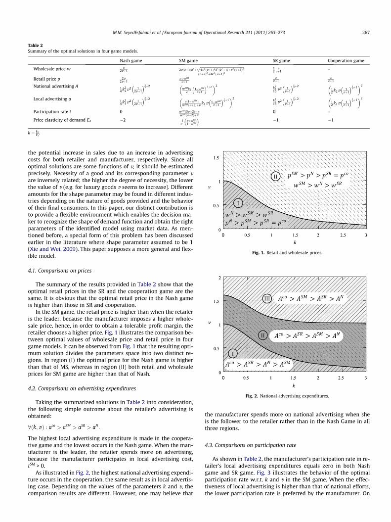
Table 2Summary of the optimal solutions in four game models.

Nash game SM game SR game Cooperation game

Wholesale price w v2vþ1 2vðvþ1Þk2þ

ffiffiffiffiffiffiffiffiffiffiffiffiffiffiffiffiffiffiffiffiffiffiffiffiffiffiffiffiffiffiffiffiffiffiffiffiffiffiffiffiffiffiffiffiffiffiffiffiffi4v2ðvþ1Þ2k2ðk2þ1Þþv2ðvþ2Þ2p

ðvþ2Þ2þ4k2ðvþ1Þ212

vvþ1

–

Retail price p 2v2vþ1

vþwSM

vþ1v

vþ1v

vþ1

National advertising A 14 k2

2v2 12vþ1

� �2vþ2

wSM k22

1�wSM

vþ1

� �1=v� �2

k22

16 v2 1vþ1

� �2vþ2

12 k2v 1

vþ1

� �1vþ1

� �2

Local advertising a 14 k2

1v2 12vþ1

� �2vþ2

vð1�wSM ÞwSM ðvþ2Þþv k1v 1�wSM

vþ1

� �1vþ1

� �2k2

116 v2 1

vþ1

� �2vþ2

12 k1v 1

vþ1

� �1vþ1

� �2

Participation rate t 0 wSM ð3vþ2Þ�vwSM ðvþ2Þþv

0 –

Price elasticity of demand Ed �2 �1v

vþwSM

1�wSM

� ��1 �1

k ¼ k2k1

.

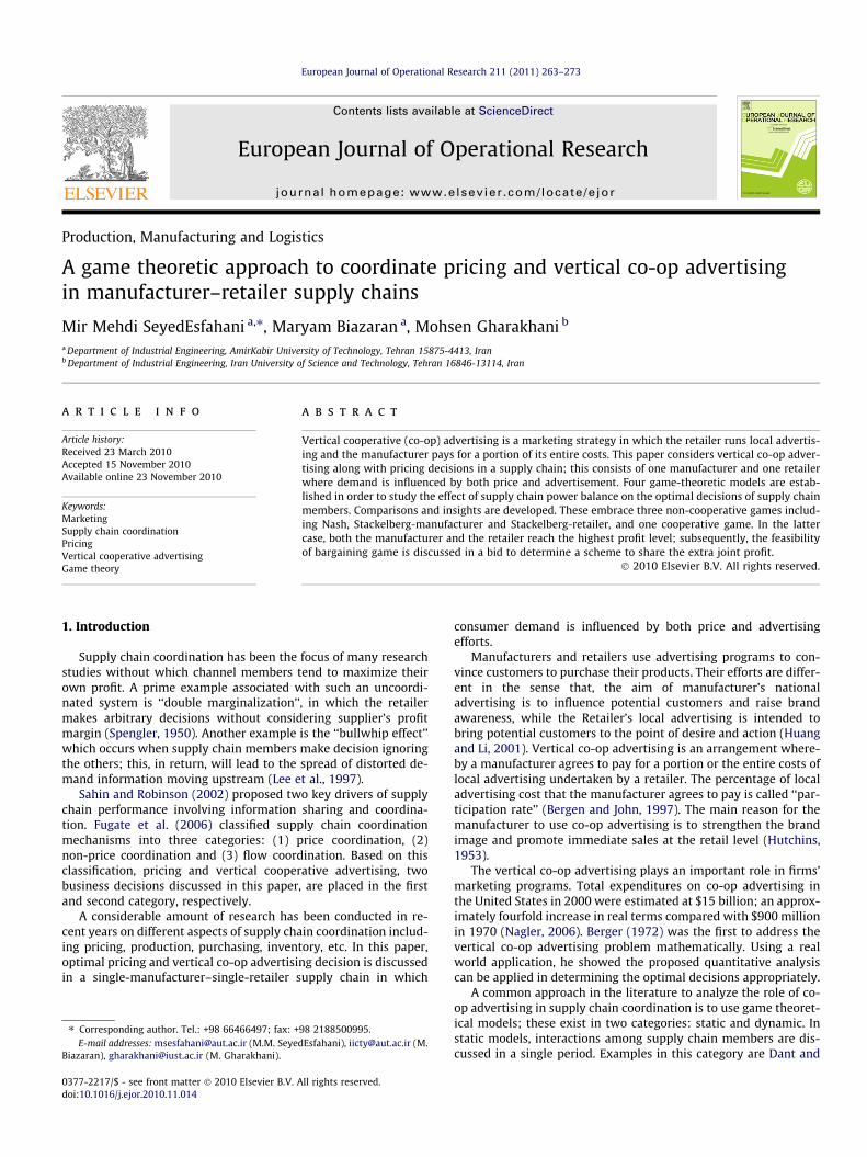
Fig. 1. Retail and wholesale prices.

Fig. 2. National advertising expenditures.

M.M. SeyedEsfahani et al. / European Journal of Operational Research 211 (2011) 263–273 267

the potential increase in sales due to an increase in advertisingcosts for both retailer and manufacturer, respectively. Since alloptimal solutions are some functions of v, it should be estimatedprecisely. Necessity of a good and its corresponding parameter vare inversely related; the higher the degree of necessity, the lowerthe value of v (e.g. for luxury goods v seems to increase). Differentamounts for the shape parameter may be found in different indus-tries depending on the nature of goods provided and the behaviorof their final consumers. In this paper, our distinct contribution isto provide a flexible environment which enables the decision ma-ker to recognize the shape of demand function and obtain the rightparameters of the identified model using market data. As men-tioned before, a special form of this problem has been discussedearlier in the literature where shape parameter assumed to be 1(Xie and Wei, 2009). This paper supposes a more general and flex-ible model.

4.1. Comparisons on prices

The summary of the results provided in Table 2 show that theoptimal retail prices in the SR and the cooperation game are thesame. It is obvious that the optimal retail price in the Nash gameis higher than those in SR and cooperation.

In the SM game, the retail price is higher than when the retaileris the leader, because the manufacturer imposes a higher whole-sale price, hence, in order to obtain a tolerable profit margin, theretailer chooses a higher price. Fig. 1 illustrates the comparison be-tween optimal values of wholesale price and retail price in fourgame models. It can be observed from Fig. 1 that the resulting opti-mum solution divides the parameters space into two distinct re-gions. In region (I) the optimal price for the Nash game is higherthan that of MS, whereas in region (II) both retail and wholesaleprices for SM game are higher than that of Nash.

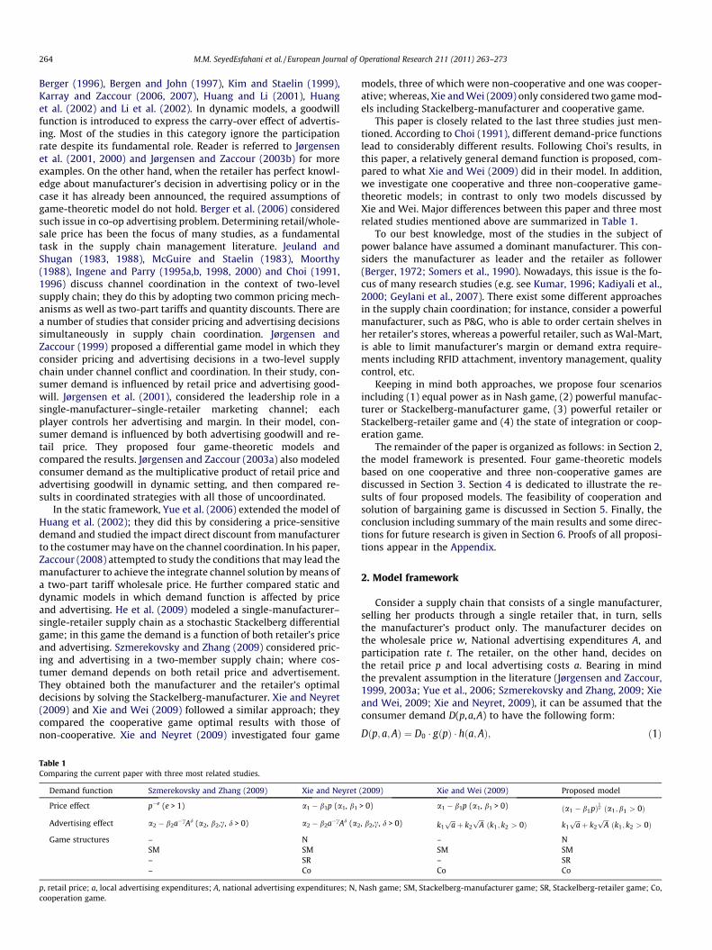
4.2. Comparisons on advertising expenditures

Taking the summarized solutions in Table 2 into consideration,the following simple outcome about the retailer’s advertising isobtained:

8ðk;vÞ : aco > aSM > aSR > aN :

The highest local advertising expenditure is made in the coopera-tive game and the lowest occurs in the Nash game. When the man-ufacturer is the leader, the retailer spends more on advertising,because the manufacturer participates in local advertising cost,tSM > 0.

As illustrated in Fig. 2, the highest national advertising expendi-ture occurs in the cooperation, the same result as in local advertis-ing case. Depending on the values of the parameters k and v, thecomparison results are different. However, one may believe that

the manufacturer spends more on national advertising when sheis the follower to the retailer rather than in the Nash Game in allthree regions.

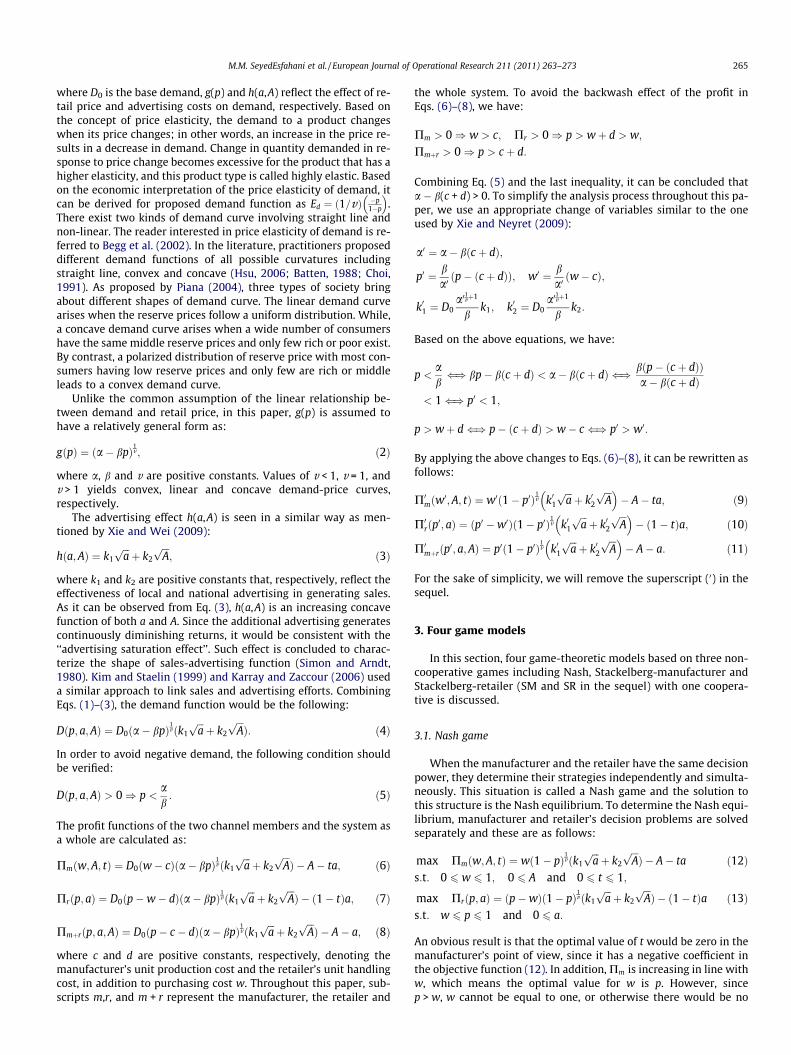
4.3. Comparisons on participation rate

As shown in Table 2, the manufacturer’s participation rate in re-tailer’s local advertising expenditures equals zero in both Nashgame and SR game. Fig. 3 illustrates the behavior of the optimalparticipation rate w.r.t. k and v in the SM game. When the effec-tiveness of local advertising is higher than that of national efforts,the lower participation rate is preferred by the manufacturer. On

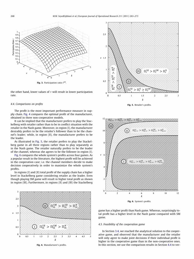
Fig. 3. Participation ratio tSM.

268 M.M. SeyedEsfahani et al. / European Journal of Operational Research 211 (2011) 263–273

the other hand, lower values of m will result in lower participationrate.

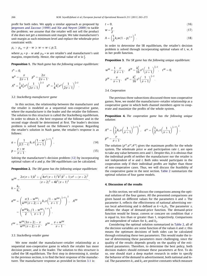
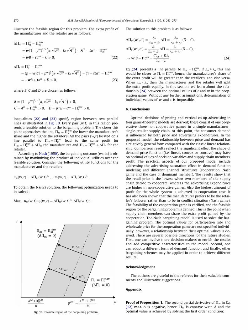
Fig. 5. Retailer’s profits.

The profit is the most important performance measure in sup-ply chain. Fig. 4 compares the optimal profit of the manufacturer,obtained in three non-cooperative models.

It can be implied that the manufacturer prefers to play the Stac-kelberg with retailer rather than to be in conflict situation with theretailer in the Nash game. Moreover, in region (I), the manufacturerdesirably prefers to be the retailer’s follower than to be the chan-nel’s leader; while, in region (II), the manufacturer prefers to bethe leader.

As illustrated in Fig. 5, the retailer prefers to play the Stackel-berg game in all three regions rather than to play separately asin the Nash game. The retailer naturally prefers to be the leaderof the channel, whereas she agrees to be the follower in region (I).

Fig. 6 compares the whole system’s profits across four games. Asa popular result in the literature, the highest profit will be achievedin the cooperation case; i.e. the channel members decide to makedecision cooperatively in order to maximize the whole system’sprofits.

In regions (I) and (II) total profit of the supply chain has a higherlevel in Stackelberg game considering retailer as the leader. Eventhough playing SM game will result in higher total profit as shownin region (III). Furthermore, in regions (II) and (III) the Stackelberg

Fig. 4. Manufacturer’s profits.

Fig. 6. System’s profits.

game has a higher profit than Nash game. Whereas, surprisingly to-tal profit has a higher level in the Nash game compared with SMgame.

4.5. Feasibility of the cooperation game

In Section 3.4, we reached the analytical solution to the cooper-ative game, and observed that the manufacturer and the retailerwill only agree to make joint decisions if their individual profit ishigher in the cooperative game than in the non-cooperative ones.In this section, we use the comparison results in Section 4.4 to ver-

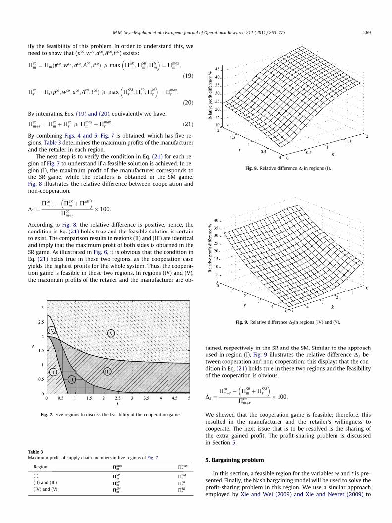
Fig. 8. Relative difference D1in regions (I).

M.M. SeyedEsfahani et al. / European Journal of Operational Research 211 (2011) 263–273 269

ify the feasibility of this problem. In order to understand this, weneed to show that (pco,wco,aco,Aco, tco) exists:

Pcom ¼ Pmðpco;wco; aco;Aco

; tcoÞP max PSMm ;PSR

m ;PNm

� �¼ Pmax

m ;

ð19Þ

Pcor ¼ Prðpco;wco; aco;Aco

; tcoÞP max PSMr ;PSR

r ;PNr

� �¼ Pmax

r :

ð20Þ

By integrating Eqs. (19) and (20), equivalently we have:

Pcomþr ¼ Pco

m þPcor P Pmax

m þPmaxr : ð21Þ

By combining Figs. 4 and 5, Fig. 7 is obtained, which has five re-gions. Table 3 determines the maximum profits of the manufacturerand the retailer in each region.

The next step is to verify the condition in Eq. (21) for each re-gion of Fig. 7 to understand if a feasible solution is achieved. In re-gion (I), the maximum profit of the manufacturer corresponds tothe SR game, while the retailer’s is obtained in the SM game.Fig. 8 illustrates the relative difference between cooperation andnon-cooperation.

D1 ¼Pco

mþr � PSRm þPSM

r

� �Pco

mþr

� 100:

According to Fig. 8, the relative difference is positive, hence, thecondition in Eq. (21) holds true and the feasible solution is certainto exist. The comparison results in regions (II) and (III) are identicaland imply that the maximum profit of both sides is obtained in theSR game. As illustrated in Fig. 6, it is obvious that the condition inEq. (21) holds true in these two regions, as the cooperation caseyields the highest profits for the whole system. Thus, the coopera-tion game is feasible in these two regions. In regions (IV) and (V),the maximum profits of the retailer and the manufacturer are ob-

Fig. 7. Five regions to discuss the feasibility of the cooperation game.

Table 3Maximum profit of supply chain members in five regions of Fig. 7.

Region Pmaxm Pmax

r

(I) PSRm PSM

r

(II) and (III) PSRm PSR

r

(IV) and (V) PSMm PSR

r

Fig. 9. Relative difference D2in regions (IV) and (V).

tained, respectively in the SR and the SM. Similar to the approachused in region (I), Fig. 9 illustrates the relative difference D2 be-tween cooperation and non-cooperation; this displays that the con-dition in Eq. (21) holds true in these two regions and the feasibilityof the cooperation is obvious.

D2 ¼Pco

mþr � PSRm þPSM

r

� �Pco

mþr

� 100:

We showed that the cooperation game is feasible; therefore, thisresulted in the manufacturer and the retailer’s willingness tocooperate. The next issue that is to be resolved is the sharing ofthe extra gained profit. The profit-sharing problem is discussedin Section 5.

5. Bargaining problem

In this section, a feasible region for the variables w and t is pre-sented. Finally, the Nash bargaining model will be used to solve theprofit-sharing problem in this region. We use a similar approachemployed by Xie and Wei (2009) and Xie and Neyret (2009) to

270 M.M. SeyedEsfahani et al. / European Journal of Operational Research 211 (2011) 263–273

illustrate the feasible region for this problem. The extra profit ofthe manufacturer and the retailer are as follows:

DPm ¼ Pcom �Pmax

m

¼ wð1� pcoÞ1=v k1

ffiffiffiffiffiffiacop

þ k2

ffiffiffiffiffiffiffiAco

p� �� Aco � taco �Pmax

m

¼ wB� taco � C > 0; ð22Þ

DPr ¼ Pcor �Pmax

r

¼ ðp�wÞð1� pcoÞ1v k1

ffiffiffiffiffiffiacop

þ k2

ffiffiffiffiffiffiffiAco

p� �� ð1� tÞaco �Pmax

r

¼ �wBþ taco þ D > 0; ð23Þ

where B, C and D are chosen as follows:

B ¼ ð1� pcoÞ1=v k1

ffiffiffiffiffiffiacop

þ k2

ffiffiffiffiffiffiffiAco

p� �> 0;

C ¼ Aco þPmaxm > 0; D ¼ pcoB� aco �Pmax

r > 0:

Inequalities (22) and (23) specify region between two parallellines as illustrated in Fig. 10. Every pair (w, t) in this region pre-sents a feasible solution to the bargaining problem. The closer thispoint approaches the line, Pm ¼ Pmax

m the lower the manufacturer’sshare and the higher the retailer’s. All the pairs (w, t) located on aline parallel to Pm ¼ Pmax

m lead to the same profit forPm ¼ Pmax

m þ DPm the manufacturer and Pr ¼ Pmaxr þ DPr for the

retailer.According to Nash (1950), the bargaining outcome (w⁄, t⁄) is ob-

tained by maximizing the product of individual utilities over thefeasible solution. Consider the following utility functions for themanufacturer and the retailer:

umðw; tÞ ¼ DPmðw; tÞkm ; urðw; tÞ ¼ DPrðw; tÞkr :

To obtain the Nash’s solution, the following optimization needs tobe solved:

Max umðw; tÞ:urðw; tÞ ¼ DPmðw; tÞkm :DPrðw; tÞkr :

Fig. 10. Feasible region of the bargaining problem.

The solution to this problem is as follows:

DPmðw�; t�Þ ¼km

km þ krDP ¼ km

km þ krðD� CÞ;

DPrðw�; t�Þ ¼kr

km þ krDP ¼ kr

km þ krðD� CÞ;

) w�B� t�aco ¼ Ckm þ Dkr

km þ kr: ð24Þ

Eq. (24) presents a line parallel to Pm ¼ Pmaxm . If km > kr, this line

would be closer to Pr ¼ Pmaxr , hence, the manufacturer’s share of

the extra profit will be greater than the retailer’s, and vice versa.When km = kr, then the manufacturer and the retailer will splitthe extra profit equally. In this section, we learn about the rela-tionship (24) between the optimal values of t and w in the coop-eration game. Without any further assumptions, determination ofindividual values of w and t is impossible.

6. Conclusions

Optimal decisions of pricing and vertical co-op advertising infour game-theoretic models are derived; these consist of one coop-erative three non-cooperative games in a single-manufacturer–single-retailer supply chain. At this point, the consumer demandis influenced by both price and advertising expenditures. In theproposed model, the relationship between price and demand hasa relatively general form compared with the classic linear relation-ship. Comparison results reflect the significant effect the shape ofdemand-price function (i.e. linear, convex or concave) may haveon optimal values of decision variables and supply chain members’profit. The practical aspects of our proposed model includeaddressing the advertising saturation effect in demand functionmodeling and different channel structures (cooperation, Nashgame and the case of dominant member). The results show thatthe retail price is the lowest when two members of the supplychain decide to cooperate, whereas the advertising expendituresare higher in non-cooperative games. Also the highest amount ofprofit for the whole system is achieved in cooperation case. Ithas also been shown that the manufacturer prefers to be the retai-ler’s follower rather than to be in conflict situation (Nash game).The feasibility of the cooperation game is verified, and the feasibleregion for the bargaining problem is defined. This is the point whensupply chain members can share the extra-profit gained by thecooperation. The Nash bargaining model is used to solve the bar-gaining problem. The optimal values for participation rate andwholesale price for the cooperation game are not specified individ-ually, however, a relationship between their optimal values is de-rived. There are several possible directions for the future studies.First, one can involve more decision-makers to enrich the resultsand add competitive characteristics to the model. Second, onecan adopt a different form of demand function and finally, otherbargaining schemes may be applied in order to achieve differentresults.

Acknowledgment

The authors are grateful to the referees for their valuable com-ments and illustrative suggestions.

Appendix

Proof of Proposition 1. The second partial derivative of Pm in Eq.(12) w.r.t. A is negative, hence, Pm is concave w.r.t. A and theoptimal value is achieved by solving the first order condition:

M.M. SeyedEsfahani et al. / European Journal of Operational Research 211 (2011) 263–273 271

@Pm

@A¼ 1

2k2wð1� pÞ

1vA�

12 � 1 ¼ 0) A ¼ 1

2k2wð1� pÞ

1v

� �2

: ðA1Þ

To solve the retailer’s problem (13), we define variable x asðp�wÞð1� pÞ

1v . To determine the domain of x, we solve the first or-

der equation below and compare the critical value with values of xat p = 0 and p = w:

@x@p¼ 1

v ð1� pÞ1v�1ðv � pðv þ 1Þ þwÞ ¼ 0) p1 ¼

v þwv þ 1

2 ðw;1Þ;

p ¼ w) x ¼ 0;

p ¼ p1 ¼v þwv þ 1

) x ¼ v 1�wv þ 1

� �1vþ1

> 0;

p ¼ 1) x ¼ 0:

Thus, the maximum of x is obtained while p = p1 and the minimumvalue of x equals zero. Now we rewrite the retailer’s decision prob-lem as follows:

max Prðx; aÞ ¼ xðk1ffiffiffiapþ k2

ffiffiffiApÞ � ð1� tÞa

s:t: 0 6 x 6 v 1�wv þ 1

� �1vþ1

and 0 6 a:

It is obvious that the retailer’s profit is increasing with x, thus, theoptimal value of x is:

x ¼ xmax ¼ v 1�wv þ 1

� �1vþ1

: ðA2Þ

It is also obvious that Pr is concave w.r.t. a; this is because the sec-ond partial derivative of Pr w.r.t. a is negative and therefore, theoptimal value of is obtained as follows:

@Pr

@a¼ 1

v k1xa�12 � ð1� tÞ ¼ 0) a ¼ 1

2ð1� tÞ k1x� �2

: ðA3Þ

Solving Eqs. (A1)–(A3) considering w ¼ p2 and t = 0, we achieve the

Nash equilibrium:

wN ¼ v2v þ 1

; pN ¼ 2v2v þ 1

; tN ¼ 0;

AN ¼ 14

k22v

2 12v þ 1

� �2vþ2

; aN ¼ 14

k21v

2 12v þ 1

� �2vþ2

:

This completes the proof of Proposition 1. h

Table A1Possible combinations of active constraints.

Possible combinationsof active constraints

combinations

No constraint is active (all ui = 0 ) 1Only one constraint is active g1,g2,g3,g4,g5,g6 6Only two constraints are

active(g1,g3), (g1,g4), (g1,g5),(g1,g6),(g2,g3), (g2,g4), (g2,g5),(g2,g6),

12

(g3,g5), (g3,g6), (g4,g5),(g4,g6),

Three constraints are active (g1,g3,g5), (g1,g3,g6),(g1,g4,g5),(g1,g4,g6), (g2,g3,g5),(g2,g3,g6),

8

(g2,g4,g5), (g2,g4,g6),Total 27

Proof of Proposition 2. Substituting Eqs. (14) and (15) into theexpression of Pm, the decision problem (12) becomes:

Max Pm ¼ w1�wv þ 1

� �1v k2

1v2ð1� tÞ

1�wv þ 1

� �1vþ1

þ k2

ffiffiffiAp

!� A

� tk21v2

4ð1� tÞ21�wv þ 1

� �2vþ2

s:t: 0 6 w 6 1; 0 6 A; 0 6 t 6 1:

Before solving this non-linear programming problem, we revise theconstraints to make sure that the objective function is continuousand differentiable in the solution area. Below comes the partialderivatives of objective function (12) w.r.t. its correspondingvariables.

@Pm

@w¼ k2

1

2ðv þ 1Þð1� tÞ1�wv þ 1

� �2v

ðv � 2wðv þ 1ÞÞ

þ k2

ffiffiffiAp

vðv þ 1Þ1�wv þ 1

� �1v�1

ðv �wðv þ 1ÞÞ

þ tk21v

2ð1� tÞ21�wv þ 1

� �2vþ1

;

@Pm

@A¼ wk2

2ffiffiffiAp 1�w

v þ 1

� �1v

� 1;

@Pm

@t¼ k2

1v4ð1� tÞ3ð1þ vÞ

1�wv þ 1

� �2vþ1

ð2wðv þ 1Þ � vð1�wÞ

� tð2wðv þ 1Þ þ vð1�wÞÞÞ:

As the partial derivatives of Pm show, this function is not differen-tiable at t = 1, w = 1 (if v > 1) and A = 0. When participation rate t ap-proaches 1, the profit function, in turn, approaches negative infinity.When w is equal to 1, the profit function equals �A < 0. We can as-sume a minimum level for the national advertising expenditures, toensure that the profit function is differentiable at this point. Thenew set of constraints is as follows:0 6 t 6 1� �t < 1;0 6 w 6 1� �w < 1;0 < �A 6 A 6 Amax;

where �t, �w, �A are positive constants and sufficiently close to zero.Amax is a positive constant, which is assumed to be as great as wedesire, employed to restrict the solution area. The new solution areais a closed and bounded set, and the objective function is definedover it. The ‘‘extreme value theorem’’ a.k.a. ‘‘Weierstrass theorem’’,states that if a real valued function is continuous over a closed andbounded set, this function must attain its minimum and maximumvalue, each at least once. Over the new set of constraints, Pm veri-fies the conditions of the ‘‘extreme value theorem’’. Thus, we canensure that there exists a solution to this problem. This solutionmust fulfill the KKT first order necessary conditions. The KKT condi-tions for this problem are as follows:

@ �Pmð Þ@w

@ �Pmð Þ@t

@ �Pmð Þ@a

0BB@

1CCAþX

6

i¼1

ui

@gi@w@gi@t@gi@a

0BB@

1CCA ¼ 0;

g1 ¼ �w 6 0; g2 ¼ w� ð1� �wÞ 6 0;g3 ¼ �t 6 0; g4 ¼ t � ð1� �tÞ 6 0;g5 ¼ �Aþ �A 6 0; g6 ¼ A� Amax 6 0;uigi ¼ 0 for i ¼ 1; . . . ;6;ui P 0 for i ¼ 1; . . . ;6:

272 M.M. SeyedEsfahani et al. / European Journal of Operational Research 211 (2011) 263–273

All the possible combinations of active constraints are shown inTable A1. The KKT necessary conditions need to be verified for eachcombination in order to achieve all candidate local maximumpoints.

Note that the constraints g1 and g2 are inconsistent; as a result,no combination with both g1 and g2 active is possible. The sameresult holds true for (g3,g4) and (g5,g6).

By verifying KKT first order necessary conditions in 27 combi-nations, only one feasible KKT point can be achieved and that iswhere no constraint is active.

All ui ¼ 0)

@ð�PmÞ@w

@ð�PmÞ@t

@ð�PmÞ@a

0BB@

1CCA ¼ 0 and All gi < 0

)

w ¼ 2vðvþ1Þk2þffiffiffiffiffiffiffiffiffiffiffiffiffiffiffiffiffiffiffiffiffiffiffiffiffiffiffiffiffiffiffiffiffiffiffiffiffiffiffiffiffiffiffiffiffiffi4v2ðvþ1Þ2k2ðk2þ1Þþv2ðvþ2Þ2pðvþ2Þ2þ4k2ðvþ1Þ2

; k ¼ k2k1; ðA4Þ

A ¼ wk22

1�wvþ1

� �1=v� �2

; ðA5Þ

t ¼ wð3vþ2Þ�vwðvþ2Þþv : ðA6Þ

8>>>>><>>>>>:

Based on the result of ‘‘extreme value theorem’’, this KKT solution isthe only local maximum candidate; hence, we conclude that thispoint is the global maximum of Pm. Therefore we obtain the SRequilibrium solving Eqs. (14) and (15) and Eqs.(A4)–(A6) as shownbelow:

wSM ¼2vðv þ 1Þk2 þ

ffiffiffiffiffiffiffiffiffiffiffiffiffiffiffiffiffiffiffiffiffiffiffiffiffiffiffiffiffiffiffiffiffiffiffiffiffiffiffiffiffiffiffiffiffiffiffiffiffiffiffiffiffiffiffiffiffiffiffiffiffiffiffiffiffiffiffiffiffiffiffiffiffiffiffiffi4v2ðv þ 1Þ2k2ðk2 þ 1Þ þ v2ðv þ 2Þ2

qðv þ 2Þ2 þ 4k2ðv þ 1Þ2

; k

¼ k2

k1;

aSM ¼ vð1�wSMÞwSMðv þ 2Þ þ v k1v

1�wSM

v þ 1

� �1vþ1

!2

; ASM

¼ wSMk2

21�wSM

v þ 1

� �1=v !2

;

tSM ¼ wSMð3v þ 2Þ � vwSMðv þ 2Þ þ v ; pSM ¼ v þwSM

v þ 1: �

Proof of Proposition 3. Substituting Eqs. (16)–(18) into theexpression of Pr , the decision problem (13) becomes:

max Prðp; aÞ ¼p2ð1� pÞ1=v k1

ffiffiffiapþ 1

4k2

2pð1� pÞ1=v� �

� a

s:t: 0 6 p 6 1 and 0 6 a:

To solve this problem, we define variable y as p2 ð1� pÞ1=v . To deter-

mine the domain of y, we solve the first order equation below andcompare the critical value of y at that specific point with values of yat p = 0 and p = 1.

@y@p¼ 1

2v ð1� pÞ1v�1ðv � pðv þ 1ÞÞ ¼ 0) p2 ¼

vv þ 1

;

p ¼ w) y ¼ 0;

p ¼ p2 ) y ¼ v2

1v þ 1

� �1vþ1

> 0;

p ¼ 1) y ¼ 0:

Hence, the maximum of y is achieved at p = p2 and the minimum va-lue of y equals zero. Now we rewrite the retailer’s decision problemas follows:

max Pr ¼ y k1ffiffiffiapþ 1

2k2

2y� �

� a

s:t: 0 6 y 6v2

1v þ 1

� �1vþ1

; 0 6 a:

We can conclude that Pr is an increasing function of y, therefore theoptimal value for y is:

y ¼ ymax ¼v2

1v þ 1

� �1vþ1

: ðA7Þ

It is also obvious that Pr is concave w.r.t. a; because the second par-tial derivative of Pr w.r.t. a is negative as shown below:

@2Pr

@a2 ¼ �14

k1ya�32 < 0:

Therefore, the optimal value of is achieved by solving the followingfirst order equation:

@Pr

@a¼ 1

2k1ya�

12 � 1 ¼ 0) a ¼ 1

2k1y

� �2

: ðA8Þ

By solving Eqs. (16)–(18), (A7) and (A8), The SR equilibrium wouldbe:

wSR ¼ 12

vv þ 1

; pSR ¼ vv þ 1

; tSR ¼ 0;

ASR ¼ k22

16v2 1

v þ 1

� �2vþ2

; aSR ¼ k21

16v2 1

v þ 1

� �2vþ2

: �

Proof of Proposition 4. To solve this problem, we define z asp(1 � p)1/v To determine the domain of z, we solve the first orderequation below and compare the value of at that point with valuesof z while p = 0 and p = 1.

@z@p¼ 1

v ð1� pÞ1v�1ðv � pðv þ 1ÞÞ ¼ 0) p3 ¼

vv þ 1

;

p ¼ w) z ¼ 0;

p ¼ p3 ¼v

v þ 1) z ¼ v 1

v þ 1

� �1vþ1

> 0;

p ¼ 1) z ¼ 0:

Hence, the maximum of z is obtained while p = p3 and the minimumvalue of z equals zero. Now we rewrite the decision problem asfollows:

max Pmþr ¼ z k1ffiffiffiapþ k2

ffiffiffiAp� �

� a� A

s:t: 0 6 z 6 v 1v þ 1

� �1vþ1

; 0 6 a and 0 6 A:

Now we derive the partial derivative of Pmþr w.r.t. z, that is:

@Pmþr

@z¼ k1

ffiffiffiapþ k2

ffiffiffiAp

> 0:

Thus, Pmþr is an increasing function of z, therefore, the optimal va-lue of z is:

z ¼ zmax ¼ v 1v þ 1

� �1vþ1

: ðA9Þ

The optimal values of a and A can be derived from the first orderconditions below:

M.M. SeyedEsfahani et al. / European Journal of Operational Research 211 (2011) 263–273 273

@Pmþr

@a¼ 1

2k1za�

12 � 1 ¼ 0) a ¼ 1

2k1z

� �2

; ðA10Þ

@Pmþr

@A¼ 1

2k2zA�

12 � 1 ¼ 0) A ¼ 1

2k2z

� �2

: ðA11Þ

The Hessian matrix is a negative definite matrix and fulfills the sec-ond-order condition for a maximum.

H ¼@2Pmþr@a2

@2Pmþr@a@A

@2Pmþr@A@a

@2Pmþr

@A2

24

35 ¼ �k1z

4affiffiap 0

0 �k2z4AffiffiAp

24

35:

Thus, the Eqs. (A9)–(A11) lead to the following solution for thecooperative game:

Aco ¼ 12

k2v1

v þ 1

� �1vþ1

!2

; aco ¼ 12

k1v1

v þ 1

� �1vþ1

!2

;

pco ¼ vv þ 1

: �

References

Batten, D., 1988. On the variable shape of the free spatial demand function. Journalof Regional Science 28 (2), 219–230.

Begg, D., Fischer, S., Dornbusch, R., 2002. Economics, seventh ed. McGraw-Hill,London.

Bergen, M., John, G., 1997. Understanding cooperative advertising participationrates in conventional channels. Journal of Marketing Research 34 (3), 357–369.

Berger, P., 1972. Vertical cooperative advertising ventures. Journal of MarketingResearch, 309–312.

Berger, P., Lee, J., Weinberg, B., 2006. Optimal cooperative advertising integrationstrategy for organizations adding a direct online channel. Journal of theOperational Research Society 57 (8), 920–927.

Choi, S., 1991. Price competition in a channel structure with a common retailer.Marketing Science, 271–296.

Choi, S., 1996. Price competition in a duopoly common retailer channel. Journal ofRetailing 72 (2), 117–134.

Dant, R., Berger, P., 1996. Modelling cooperative advertising decisions infranchising. Journal of the Operational Research Society, 1120–1136.

Fugate, B., Sahin, F., Mentzer, J., 2006. Supply chain management coordinationmechanisms. Journal of Business Logistics 27 (2), 129.

Geylani, T., Dukes, A., Srinivasan, K., 2007. Strategic manufacturer response to adominant retailer. Marketing Science 26 (2), 164.

He, X., Prasad, A., Sethi, S., 2009. Cooperative advertising and pricing in a dynamicstochastic supply chain: Feedback Stackelberg strategies. Production andOperations Management 18 (1), 78–94.

Hsu, S., 2006. Simple monopoly price theory in a spatial market. The Annals ofRegional Science 40 (3), 531–544.

Huang, Z., Li, S., 2001. Co-op advertising models in manufacturer–retailer supplychains: A game theory approach. European Journal of Operational Research 135(3), 527–544.

Huang, Z., Li, S., Mahajan, V., 2002. An analysis of manufacturer–retailer supplychain coordination in cooperative advertising. Decision Sciences 33 (3), 469–494.

Hutchins, M., 1953. Cooperative Advertising: Roland Press, New York.Ingene, C., Parry, M., 1995a. Channel coordination when retailers compete.

Marketing Science 14 (4), 360–377.Ingene, C., Parry, M., 1995b. Coordination and manufacturer profit maximization:

The multiple retailer channel. Journal of Retailing 71 (2), 129–151.Ingene, C., Parry, M., 1998. Manufacturer-optimal wholesale pricing when retailers

compete. Marketing Letters 9 (1), 65–77.

Ingene, C., Parry, M., 2000. Is channel coordination all it is cracked up to be? Journalof Retailing 76 (4), 511–547.

Jeuland, A., Shugan, S., 1983. Managing channel profits. Marketing Science, 239–272.

Jeuland, A., Shugan, S., 1988. Channel of distribution profits when channel membersfrom conjectures. Marketing Science, 202–210.

Jørgensen, S., Sigue, S., Zaccour, G., 2001. Stackelberg leadership in a marketingchannel. International Game Theory Review 3 (1), 13–26.

Jørgensen, S., Sigue, S., Zaccour, G., 2000. Dynamic cooperative advertising in achannel. Journal of Retailing 76 (1), 71–92.

Jørgensen, S., Zaccour, G., 1999. Equilibrium pricing and advertising strategies in amarketing channel. Journal of Optimization Theory and Applications 102 (1),111–125.

Jørgensen, S., Zaccour, G., 2003a. Channel coordination over time: Incentiveequilibria and credibility. Journal of Economic Dynamics and Control 27 (5),801–822.

Jørgensen, S., Zaccour, G., 2003b. A differential game of retailer promotions.Automatica 39 (7), 1145–1155.

Kadiyali, V., Chintagunta, P., Vilcassim, N., 2000. Manufacturer–retailer channelinteractions and implications for channel power: An empirical investigation ofpricing in a local market. Marketing Science 19 (2), 127–148.

Karray, S., Zaccour, G., 2006. Could co-op advertising be a manufacturer’scounterstrategy to store brands? Journal of Business research 59 (9), 1008–1015.

Karray, S., Zaccour, G., 2007. Effectiveness of coop advertising programs incompetitive distribution channels. International Game Theory Review 9 (2),151.

Kim, S., Staelin, R., 1999. Manufacturer allowances and retailer pass-through ratesin a competitive environment. Marketing Science, 59–76.

Kumar, N., 1996. The power of trust in manufacturer–retailer relationships. HarvardBusiness Review 74, 92–110.

Lee, H., Padmanabhan, V., Whang, S., 1997. Information distortion in a supply chain:the bullwhip effect. Management Science 43 (4), 546–558.

Li, S., Huang, Z., Zhu, J., Chau, P., 2002. Cooperative advertising, game theory andmanufacturer–retailer supply chains. Omega 30 (5), 347–357.

McGuire, T., Staelin, R., 1983. An industry equilibrium analysis of downstreamvertical integration. Marketing Science 2 (2), 161–191.

Moorthy, K., 1988. Strategic decentralization in channels. Marketing Science 7 (4),335–355.

Nagler, M., 2006. An exploratory analysis of the determinants of cooperativeadvertising participation rates. Marketing Letters 17 (2), 91–102.

Nash Jr., J., 1950. The bargaining problem. Econometrica: Journal of the EconometricSociety 18 (2), 155–162.

Piana, V., 2004. Consumer Decision Rules for Agent-Based Models. Economics WebInstitute.

Sahin, F., Robinson, E., 2002. Flow coordination and information sharing in supplychains: Review, implications, and directions for future research. DecisionSciences 33 (4), 505–536.

Simon, J., Arndt, J., 1980. The shape of the advertising response function. Journal ofAdvertising Research 20 (4), 11–28.

Somers, T., Gupta, Y., Herriott, S., 1990. Analysis of cooperative advertisingexpenditures: A transfer-function modeling approach. Journal of AdvertisingResearch 30 (1), 35–45.

Spengler, J., 1950. Vertical integration and antitrust policy. The Journal of PoliticalEconomy 58 (4), 347–352.

Szmerekovsky, J., Zhang, J., 2009. Pricing and two-tier advertising with onemanufacturer and one retailer. European Journal of Operational Research 192(3), 904–917.

Xie, J., Neyret, A., 2009. Co-op advertising and pricing models in manufacturer–retailer supply chains. Computers & Industrial Engineering 56 (4), 1375–1385.

Xie, J., Wei, J., 2009. Coordinating advertising and pricing in a manufacturer–retailerchannel. European Journal of Operational Research 197 (2), 785–791.

Yue, J., Austin, J., Wang, M., Huang, Z., 2006. Coordination of cooperative advertisingin a two-level supply chain when manufacturer offers discount. EuropeanJournal of Operational Research 168 (1), 65–85.

Zaccour, G., 2008. On the coordination of dynamic marketing channels and two-parttariffs. Automatica 44 (5), 1233–1239.