A fuzzy multi-criteria decision making approach for ...

HAL Id: hal-01758604https://hal.archives-ouvertes.fr/hal-01758604

Submitted on 4 Apr 2018

HAL is a multi-disciplinary open accessarchive for the deposit and dissemination of sci-entific research documents, whether they are pub-lished or not. The documents may come fromteaching and research institutions in France orabroad, or from public or private research centers.

L’archive ouverte pluridisciplinaire HAL, estdestinée au dépôt et à la diffusion de documentsscientifiques de niveau recherche, publiés ou non,émanant des établissements d’enseignement et derecherche français ou étrangers, des laboratoirespublics ou privés.

A fuzzy multi-criteria decision making approach formanaging performance and risk in integrated

procurement-production planningRihab Khemiri, Khaoula Elbedoui-Maktouf, Bernard Grabot, Belhassen

Zouari

To cite this version:Rihab Khemiri, Khaoula Elbedoui-Maktouf, Bernard Grabot, Belhassen Zouari. A fuzzy multi-criteriadecision making approach for managing performance and risk in integrated procurement-productionplanning. International Journal of Production Research, Taylor & Francis, 2017, vol. 55 (n°18), pp.5305-5329. �10.1080/00207543.2017.1308575�. �hal-01758604�

https://hal.archives-ouvertes.fr/hal-01758604

https://hal.archives-ouvertes.fr

To link to this article: DOI:10.1080/00207543.2017.1308575 URL:https://doi.org/10.1080/00207543.2017.1308575

This is an author-deposited version published in: http://oatao.univ-toulouse.fr/ Eprints ID: 19719

To cite this version: Khemiri, Rihab and Elbedoui-Maktouf, Khaoula and Grabot, Bernard and Zouari, Belhassen A fuzzy multi-criteria decision making approach for managing performance and risk in integrated procurement-production planning. (2017) International Journal of Production Research, vol. 55 (n°18). pp. 5305-5329. ISSN 0020-7543

Open Archive Toulouse Archive Ouverte (OATAO) OATAO is an open access repository that collects the work of Toulouse researchers and makes it freely available over the web where possible.

Any correspondence concerning this service should be sent to the repository administrator: [email protected]

A fuzzy multi-criteria decision-making approach for managing performance and risk in

integrated procurement–production planning

Rihab Khemiria,b,c, Khaoula Elbedoui-Maktouf a, Bernard Grabotb* and Belhassen Zouaric

aFaculty of Sciences of Tunis, University of Tunis El Manar, Tunis, Tunisia; bLGP, INPT-ENIT, Université de Toulouse, Tarbes Cedex,France; cMediatron Lab, Higher School of Communications of Tunis, University of Carthage, Carthage, Tunisia

Nowadays in Supply Chain (SC) networks, a high level of risk comes from SC partners. An effective risk managementprocess becomes as a consequence mandatory, especially at the tactical planning level. The aim of this article is topresent a risk-oriented integrated procurement–production approach for tactical planning in a multi-echelon SC networkinvolving multiple suppliers, multiple parallel manufacturing plants, multiple subcontractors and several customers. Anoriginality of the work is to combine an analytical model allowing to build feasible scenarios and a multi-criteriaapproach for assessing these scenarios. The literature has mainly addressed the problem through cost or profit-basedoptimisation and seldom considers more qualitative yet important criteria linked to risk, like trust in the supplier,flexibility or resilience. Unlike the traditional approaches, we present a method evaluating each possible supply scenariothrough performance-based and risk-based decision criteria, involving both qualitative and quantitative factors, in orderto clearly separate the performance of a scenario and the risk taken if it is adopted. Since the decision-maker oftencannot provide crisp values for some critical data, fuzzy sets theory is suggested in order to model vague informationbased on subjective expertise. Fuzzy Technique for Order of Preference by Similarity to Ideal Solution is used to deter-mine both the performance and risk measures correlated to each possible tactical plan. The applicability and tractabilityof the proposed approach is shown on an illustrative example and a sensitivity analysis is performed to investigate theinfluence of criteria weights on the selection of the procurement–production plan.

Keywords: procurement; supply chain management; multi-criteria decision-making; risk management; fuzzy sets theory;fuzzy logic

1. Introduction

Supply Chain Planning (SCP) is one of the most important issues in Supply Chain Management (SCM) (Gupta and

Maranas 2003). Three decision levels can be distinguished in SC planning: strategic, tactical and operational (Gupta and

Maranas 1999). Strategic planning deals with long-term decisions, from two to ten years, concerning the design of the

SC and its configuration (Chauhan, Nagi, and Proth 2004; Kemmoe, Pernot, and Tchernev 2014). Tactical decisions are

made in the medium-term horizon, between three months and two years (Chhaochhria and Graves 2013; Khakdaman

et al. 2015), in order to optimally use the resources and determine production and procurement quantities for the whole

SC. Operational decisions are made with a short-term horizon, from one to two weeks, and mainly concern the exact

scheduling of the detailed tasks according to various resource constraints (Baumann and Trautmann 2013; Wang, Liu,

and Chu 2015; Ivanov et al. 2016). This article focuses on tactical planning.

Traditionally, procurement and production activities are handled separately. However, the ordered quantities of raw

materials depend on the production quantities of finished product. Therefore, separating these two activities may result

in sub optimisation and poor overall performance (Goyal and Deshmukh 1992).

Three paramount characteristics of the integrated procurement–production planning problems should be taken into

account by the decision-maker: (i) The rapid market changes may result in conflicting objectives regarding performance

maximisation and risk minimisation. (ii) The complex nature of the relationships amongst the different actors on the SC

results in a high degree of uncertainty in the tactical planning decisions. (iii) Some input data and preferences are only

accessible through human judgments or uncertain data that can hardly be estimated by crisp numerical values or by

probability distributions.

However, few research works simultaneously consider all these issues. The majority of the existing literature

addresses the integration of the planning activities as an optimisation process, oriented on cost minimisation (see for

*Corresponding author. Email: [email protected]

instance (Su and Lin 2015; Gholamian et al. 2015; Gholamian, Mahdavi, and Tavakkoli-Moghaddam 2016; Giri,

Bardhan, and Maiti 2016)), and do not address qualitative (but important) evaluation criteria linked to the risk correlated

to each procurement–production alternative, especially when changes occur.

Even if many approaches have been defined for coping with uncertainty, most of them are based on probability dis-

tributions, requiring knowledge on historical data. When such information is not available, fuzzy set theory (Gholamian,

Mahdavi, and Tavakkoli-Moghaddam 2016), possibility theory (Torabi and Hassini 2008) and Dempster–Shafer Theory

(Curcurù, Galante, and La Fata 2013) may help to deal with both epistemic uncertainty and subjective information.

In this context, the aim of this paper is to propose and test an integrated procurement–production planning system

for a multi-echelon SC with multiple parallel manufacturing plants, multiple suppliers, multiples subcontractors and

several customer zones, involving quantitative and qualitative criteria linked to performance and risk. Multi-Criteria

Decision-Making (MCDM) techniques can provide a suitable base for the assessment phase. Within this framework, we

suggest to model qualitative criteria, mostly evaluated using human judgments, by trapezoidal fuzzy numbers (Chou,

Chang, and Shen 2008).

Bellman and Zadeh (1970) have been the first ones to integrate Fuzzy Set theory with MCDM as an effective

approach to deal with the vagueness of the human decision-making process. Fuzzy Technique for Order of Preference

by Similarity to Ideal Solution (fuzzy-TOPSIS) (Chen 2000) will be used in this article to rank the alternatives planning

under evaluation.

This article has three main contributions. Firstly, it suggests an analytical model allowing to generate the set of pro-

curement–production scenarios allowing to satisfy the demand in the context of multiple parallel manufacturing plants,

multiple suppliers, multiples subcontractors and multiple customer zones. Secondly, it introduces risk-based criteria,

often neglected in the existing contributions, in the procurement–production problem. Thirdly, it proposes a multi-criteria

decision support approach providing independent measures of the performance and risk correlated to each procurement–

production scenario.

The article is structured as follows. The relevant literature is explored in next section. Section 3 suggests various

decision criteria for evaluating allocation scenarios. Section 4 introduces the theoretical background of this work while

Section 5 presents the structure of the SC and the considered problem. In Section 6, the proposed multi-criteria deci-

sion-making approach is detailed, an illustrative example being presented in Section 7. Finally, a sensitivity analysis is

performed to investigate the importance of the weights of the criteria on the decision-making process.

2. Literature review

This short survey is mainly oriented on the two problems to solve: the integrated procurement–production planning

problem, and the decision criteria that can be used for the supplier selection and order allocation problems.

2.1 Tactical supply chain planning

A wide variety of tactical planning models has been developed in the scientific literature on SCM, and may be classified

according to the characteristics of the physical system (i.e. single plant/multiple plants), to the domain of decision (i.e.

production, distribution and procurement), and to the data used (crisp/deterministic vs. imprecise/stochastic data). When

deterministic data cannot be found, a large number of studies use stochastic programming (Gupta and Maranas 2003;

Kazemi Zanjani, Nourelfath, and Ait-Kadi 2010) or robust optimisation (Kanyalkar and Adil 2010; Mirzapour

Al-e-hashem, Malekly, and Aryanezhad 2011; Niknamfar, Niaki, and Pasandideh 2015). In this case, probability distri-

butions are usually deduced from historical data. However, in practice, providing a realistic probability distribution is

not easy. Nevertheless, the actors of the company often have a good practical expertise that can be reused. Fuzzy Sets

Theory can be an efficient tool for modelling such subjective data, and has been used in that purpose in several recent

researches related to tactical SCP, e.g. for production planning (Wang and Liang 2005; Chen and Huang 2010), or for

dealing with the interrelations between distribution and production (Liang 2008; Selim, Araz, and Ozkarahan 2008;

Torabi and Moghaddam 2011). Among the rare studies modelling uncertainties by fuzzy sets for integrated

procurement–production planning, (Chen and Chang 2006) suggests a multi-product, multi-period and multi-echelon SC

model for reducing costs when the demand, the unitary cost of raw materials and the unitary transportation cost of prod-

ucts are modelled by fuzzy numbers. Torabi and Hassini (2008) developed a multi-objective possibilistic mixed integer

linear programming model to formulate an integrated procurement, production and distribution planning problem in a

fuzzy environment for a three echelon SC consisting of multiple suppliers, one manufacturer and multiple distribution

centres. The proposed model uses two objectives functions: minimisation of the total cost of logistics and maximisation

of the total value of purchasing. The latter considers the impact of qualitative criteria related to purchasing decisions,

such as technical capacities of the suppliers, business structure and after sale services. However, in spite of the

subjective nature of these criteria, they are assessed quantitatively. This work was extended in (Torabi and Hassini

2009) by proposing an interactive fuzzy goal programming approach for a multi echelon SC in presence of imprecise

data, such as market demand and available capacities. As in their previous work (Torabi and Hassini 2008), the authors

evaluate subjective criteria using quantitative measurements.

Peidro et al. (2009) introduced a fuzzy mixed-integer linear programming model for integrating procurement,

production and distribution planning where supply, demand and process are modelled by triangular fuzzy numbers. The

target is the best use of the available resources while meeting customer demand at minimum cost. The authors

developed a strategy for transforming the fuzzy formulation into an equivalent axillary crisp mixed integer linear pro-

gramming model.

Recently, Gholamian et al. (2015) developed a fuzzy multi-objective mixed integer nonlinear programme for a

multi-echelon SC. Four objective functions were suggested: (i) minimising the total cost, (ii) improving the customer

satisfaction, (iii) minimising the rate of changes of the workforce and (iv) maximising the total value of purchasing. The

first three conflicting criteria were reused in (Gholamian, Mahdavi, and Tavakkoli-Moghaddam 2016) to formulate a

mixed integer nonlinear programme for an integrated tactical and operational planning, solved by fuzzy optimisation.

We can observe that a limited number of studies deal with integrated procurement–production planning. Moreover,

these studies mainly suggest the use of mathematical optimisation approaches, the objectives at the mid-term horizon

being usually limited to meeting the customer demands and minimising the total cost / maximising the total profit.

These approaches do not consider subjective criteria, or convert them into quantitative ones. Indeed, even if the presence

of imprecise / expert data is recognised as an important characteristic of such planning problems, few studies suggest

using the available expert knowledge.

Another important limitation is that these methods do not include risk management in their decision process. Indeed,

they limit the awareness on risk to the existence of some uncertain parameters, such as market demand, supply, produc-

tion process and their associated costs and do not consider explicitly the characteristics and behaviour of the partners of

the SC (suppliers, plants, etc.) facing risk.

In the following sub-section, a short review of the most frequently used decision criteria in supplier selection and

order allocation processes is given.

2.2. Supplier selection and order allocation problem

Supplier selection is an important strategic decision in SCM. Many criteria, either quantitative or qualitative, have been

proposed since 1966, such as quality, productive capability, price, delivery, industry position, financial stability, perfor-

mance history, reputation, location, reliability, responsiveness, safety, customer responsiveness, relationship closeness,

etc. (Weber, Current, and Benton 1991; Dickson 1966; Huang and Keskar 2007). Nevertheless, most studies suggest that

product quality, price and delivery time are the most important ones (Shipley 1985; Ellram 1990; Pi and Low 2005).

We think that this is not anymore true in an ever-changing context in which the execution of an optimal planning may

be set into question by unexpected events.

The allocation of the orders to the selected suppliers should also be optimised. (Guneri, Yucel, and Ayyildiz 2009)

presents an integrated fuzzy linear programming approach to solve the multiple sourcing supplier selection problem

under uncertainty and vagueness. The proposed approach uses trapezoidal fuzzy numbers to evaluate importance weights

and ratings of supplier selection criteria including reputation and position, relationship closeness, performance history,

delivery capability and conflict resolution. As a second step, a linear programming model is presented to select the best

suppliers and the optimal order quantities, considering the objective of total value purchase maximisation and constraints

such as quality, budget and capacity.

Mafakheri, Breton, and Ghoniem (2011) suggest a two stage multiple criteria dynamic programming approach to

solve the supplier selection and order allocation problem. In the first stage, Analytic Hierarchy Process (AHP) (Saaty

1980) is used to rank potential suppliers using four criteria (quality, price performance, delivery performance and

environmental performance) decomposed into 21 qualitative and quantitative sub-criteria. Then, an order allocation

model is proposed on the basis of two objectives: minimising the total SC costs and maximising the utility function for

the company.

In (Arabzad et al. 2015), suppliers are evaluated using a Strengths, Weaknesses, Opportunities and Threats analysis

according to quantitative and qualitative criteria. Fuzzy TOPSIS is then used to determine the weights of the criteria. In

the second phase, the results provided by Fuzzy TOPSIS are used as input for a mixed integer linear programming

calculating the allocated order to each supplier. The model is solved using LINGO.

Zouggari and Benyoucef (2012) also proposed a two-phase decision-making approach for supplier selection, then

order allocation. In the first phase, Fuzzy-AHP is used to select suppliers based on four classes of criteria (performance

strategy, quality of service, innovation and risk), qualitatively evaluated. In the second phase, Fuzzy TOPSIS is used to

assess the order allocation among the selected suppliers on the base of three criteria (cost, quality and delivery). This

article is one of the few taking explicitly ‘risk’ into account, but only strategic risks are considered, linked to the geo-

graphical location of the supplier and the political and economic stability of its country. However, risks can also occur

at the tactical level, linked to the poor flexibility of a supplier for instance, that may become a problem if changes are

required. Consequently, it is in our opinion important to consider risk factors not only when selecting the suppliers but

also when allocating them the orders.

It can be seen that the majority of existing studies on the supplier selection problem with order allocation are exclu-

sively based on performance criteria. Factors of risk like poor flexibility of the supplier, low commitment, or fragility

are not considered at middle term. When present, the criteria related to risk are generally aggregated with others in order

to compute an overall score for each supplier. In our opinion, they should be clearly distinguished from criteria linked

to performance, since they provide information of different nature. They should therefore be displayed without a priori

aggregation, so that the decision-maker can distinguish these two dimensions of a plan.

To overcome the various limitations described above, we suggest developing a tactical planning method based on

both performance and risk decision criteria, clearly distinguished from each other and efficiently captured through expert

knowledge. To achieve this goal, a multi-criteria decision-making approach is used and several novel decision criteria

are proposed.

3. Proposed decision criteria

We suggest in what follows a list of sub-criteria allowing assessing the performance and risk of a procurement–

production plan. Nevertheless, the list should be adapted in order to fit with the specificity of a given real case.

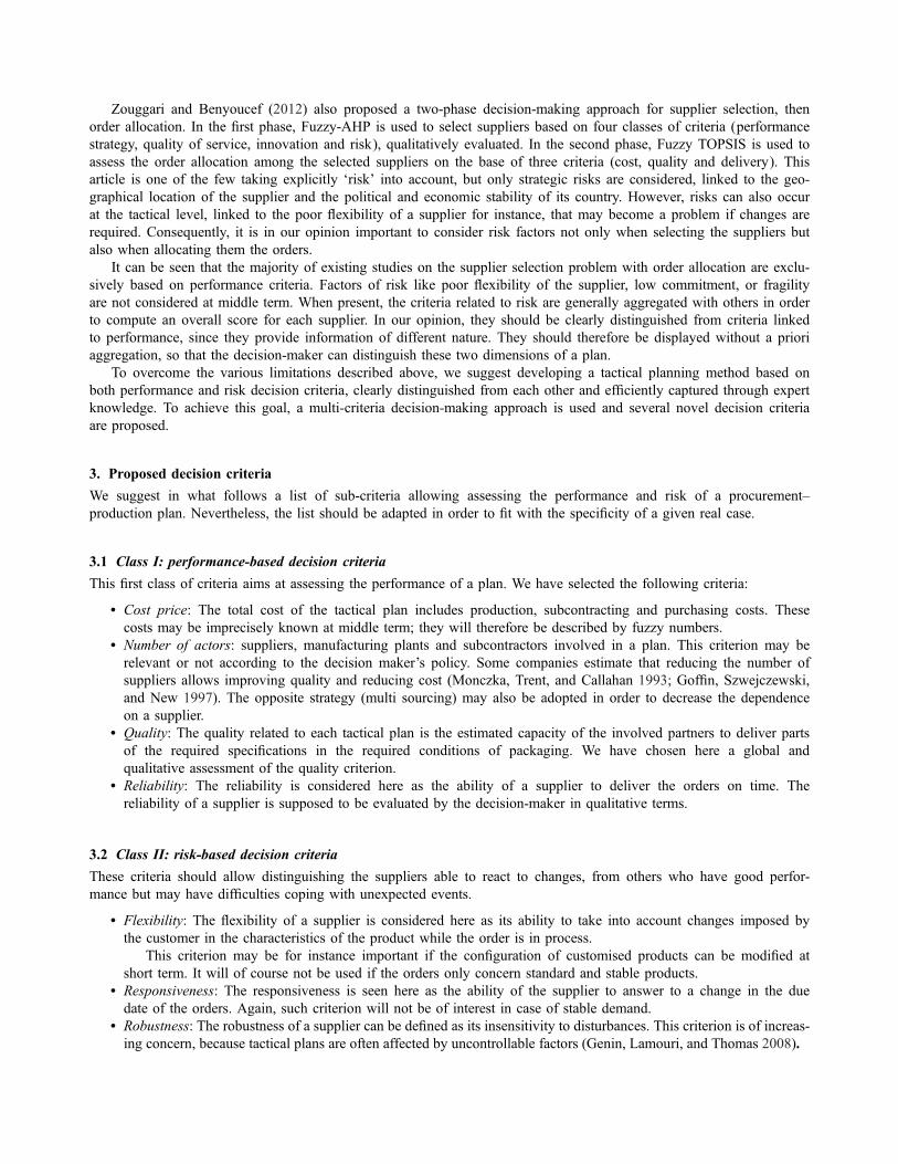
3.1 Class I: performance-based decision criteria

This first class of criteria aims at assessing the performance of a plan. We have selected the following criteria:

• Cost price: The total cost of the tactical plan includes production, subcontracting and purchasing costs. These

costs may be imprecisely known at middle term; they will therefore be described by fuzzy numbers.

• Number of actors: suppliers, manufacturing plants and subcontractors involved in a plan. This criterion may be

relevant or not according to the decision maker’s policy. Some companies estimate that reducing the number of

suppliers allows improving quality and reducing cost (Monczka, Trent, and Callahan 1993; Goffin, Szwejczewski,

and New 1997). The opposite strategy (multi sourcing) may also be adopted in order to decrease the dependence

on a supplier.

• Quality: The quality related to each tactical plan is the estimated capacity of the involved partners to deliver parts

of the required specifications in the required conditions of packaging. We have chosen here a global and

qualitative assessment of the quality criterion.

• Reliability: The reliability is considered here as the ability of a supplier to deliver the orders on time. The

reliability of a supplier is supposed to be evaluated by the decision-maker in qualitative terms.

3.2 Class II: risk-based decision criteria

These criteria should allow distinguishing the suppliers able to react to changes, from others who have good perfor-

mance but may have difficulties coping with unexpected events.

• Flexibility: The flexibility of a supplier is considered here as its ability to take into account changes imposed by

the customer in the characteristics of the product while the order is in process.

This criterion may be for instance important if the configuration of customised products can be modified at

short term. It will of course not be used if the orders only concern standard and stable products.

• Responsiveness: The responsiveness is seen here as the ability of the supplier to answer to a change in the due

date of the orders. Again, such criterion will not be of interest in case of stable demand.

• Robustness: The robustness of a supplier can be defined as its insensitivity to disturbances. This criterion is of increas-

ing concern, because tactical plans are often affected by uncontrollable factors (Genin, Lamouri, and Thomas 2008).

• Resilience: Resilience is sometimes defined as the ability of the actor to get back to its original state after disruption

(Mensah and Merkuryev 2014), but this definition is in our opinion too close to the one of robustness. According to

Bhamra, Dani, and Burnard (2011), resilience is the ability of an entity to return to a stable state after disruption. In

psychology, resilience is the ability of an individual to reach a satisfactory state (even if different from the one initially

expected) after a crisis (Cyrulnik and Macey 2009). We select this definition here.

In recent years, there has been a considerable academic interest in SC resilience (Tukamuhabwa et al. 2015).

However, only few studies integrate the resilience criterion into the supplier selection process (Haldar et al. 2012,

2014; Sahu, Datta, and Mahapatra 2016). To our best knowledge, none considers it for order allocation.

• Stability: The stability of a supplier is linked to the planning more than to the supplier itself: it expresses the stability

of the load of the supplier between two consecutive periods. Practical studies have shown that a supplier (especially a

small one) can be destabilised by important load variations (Ming, Grabot, and Houé 2014), leading to an increased

risk to be unable to fulfil the orders. We shall assess this criterion by calculating the difference between the previous

and the actual load, therefore estimating an instability measure that should be minimised.

Quality, reliability, flexibility, responsiveness, robustness and resilience are benefit criteria (to be maximised),

whereas cost price, number of actors and instability are cost criteria (to be minimised).

Except the instability criterion, all these criteria will be qualitatively assessed according to an expert judgement.

In next sections are provided the theoretical bases allowing using these criteria for assessing a supplier, then a pro-

curement–production plan.

4. Theoretical background

4.1 Multi-criteria decision-making methods

Several methods have been proposed to deal with multi-criteria assessment problems, frequently classified according to

the discrete or continuous nature of the alternatives. A discrete problem (Multi Attribute Decision Making (MADM))

usually consists of a limited number of decision alternatives, whereas a continuous problem (Multi Objective Decision

Making) deals with a large or infinite amount of alternatives. The main proposal of this study is to evaluate each pre-

specified procurement–production plan through performance-based and risk-based decision criteria. The decision-making

problem has thus a discrete nature and a MADM method will be adequate in this case. MADM methods may be cate-

gorised according to their compensatory or non-compensatory nature. The compensatory methods are based on multi-

attribute value functions and Multi-Attribute Utility Theory (MAUT) and use an aggregation of the criteria. In contrast,

the non-compensatory methods are mainly based on an outranking relation, which consists in the comparison between

the alternatives according to each individual criterion. PROMETHEE (Brans and Vincke 1985) and ELECTRE (Roy

and Bertier 1971; Roy 1978) are the most prevalent outranking methods. However, it has been acknowledged that such

methods are able to provide a partial ranking among alternatives, but not a global one. Accordingly, MAUT methods

are considered in this paper. Among these methods, we can cite for example AHP (Saaty 1980), Technique for Order of

Preference by Similarity to Ideal Solution (TOPSIS) (Hwang and Yoon 1981), VIsekriterijumska optimizacija i

KOmpromisno Resenje (VIKOR) (Opricovic 1998), COmplex PRoportional ASsessment (COPRAS) (Zavadskas,

Kaklauskas, and Sarka 1994), Multi-Attributive Border Approximation Area Comparison (MABAC) (Pamučar and

Ćirović 2015; Gigović et al. 2017) and Multi-Attributive Ideal-Real Comparative Analysis (MAIRCA) (Pamučar, Vasin,

and Lukovac 2014; Gigović et al. 2016).

Each method has its advantages and drawbacks, including its complexity of use. In this study, TOPSIS is chosen for

the four advantages cited in Kim, Park, and Yoon (1997) and Shih, Shyur, and Lee (2007): (i) a sound logic that charac-

terises the rationale of human choice; (ii) a scalar number calculated on the basis of both the worst and the best alterna-

tives simultaneously; (iii) a simple computation method that can be readily programmed in a spread sheet; and (iv) the

performance measures of each alternative on the various attributes can be presented on a polyhedron, at least for two

dimensions. In addition, TOPSIS (but it is also the case for the aforementioned methods) has been extended for dealing

with fuzzy criteria or weights (Triantaphyllou and Lin 1996; Chen 2000).

Thus, Fuzzy TOPSIS, described with more details in Section 4.3, is used for evaluating the performance and the risk

correlated to each alternative planning, through several quantitative and qualitative criteria.

4.2 Fuzzy set theory

Fuzzy set theory was introduced by Zadeh (1965) for representing the inherent imprecision, uncertainty and vagueness

of subjective information. Trapezoidal fuzzy numbers are used here to represent the imprecise data: this restriction

allows simple calculations, and it has often been shown that this modelling framework is sufficient for modelling expert

knowledge (Chou, Chang, and Shen 2008).

Definition 1: A trapezoidal fuzzy number ~z1can be represented as a quadruplet of real numbers (a1, b1, c1, d1) as shown

in Figure 1.

Definition 2: Given two fuzzy trapezoidal fuzzy numbers ~z1 = (a1, b1, c1, d1) and ~z2 = (a2, b2, c2, d2) and any positive

real number r, the main operations on fuzzy numbers can be defined as follows (Chen, Lin, and Huang 2006):

~z1 ! ~z2 ¼ ða1 þ a2; b1 þ b2; c1 þ c2; d1 þ d2Þ (1)

~z1 H ez2 ¼ ða1 & d2; b1 & c2; c1 & b2; d1 & a2Þ (2)

~z1 ' ~z2 ¼ ða1 ( a2; b1 ( b2; c1 ( c2; d1 ( d2Þ (3)

~z1 ' r ¼ ða1 ( r; b1 ( r; c1 ( r; d1 ( rÞ (4)

Definition 3: Let ~z1 = (a1, b1, c1, d1) and ~z2 = (a2, b2, c2, d2) be two trapezoidal fuzzy numbers; the distance between

them can be calculated using the vertex method (Chen 2000; Chen, Lin, and Huang 2006):

Dð~z1;~z2Þ ¼

ffiffiffiffiffiffiffiffiffiffiffiffiffiffiffiffiffiffiffiffiffiffiffiffiffiffiffiffiffiffiffiffiffiffiffiffiffiffiffiffiffiffiffiffiffiffiffiffiffiffiffiffiffiffiffiffiffiffiffiffiffiffiffiffiffiffiffiffiffiffiffiffiffiffiffiffiffiffiffiffiffiffiffiffiffiffiffiffiffiffiffiffiffiffiffiffiffi1

4½ a1 & a2ð Þ2þ b1 & b2ð Þ2þ c1 & c2ð Þ2þ d1 & d2ð Þ2*

r(5)

Definition 4: A matrix eD is called a fuzzy matrix if it includes at least a fuzzy entry (Buckley 1985).

Definition 5: A linguistic variable is a variable which value is presented in linguistic terms (Zimmermann 2011).

Linguistic variables are commonly used to express subjective or qualitative appreciation of a decision-maker, using

terms such as ‘very low’, ‘low’, ‘medium’, ‘high’, etc. Linguistic values can be modelled by fuzzy numbers.

4.3 From TOPSIS to Fuzzy TOPSIS

To compare solutions, TOPSIS computes the distance from each alternative to the Positive Ideal Solution (PIS) and

Negative Ideal Solution (NIS). The PIS (resp. NIS) is the solution that minimises (resp. maximises) the ‘cost’ criteria

and maximises (resp. minimises) the ‘benefit’ criteria (‘cost’ and ‘benefit’ are considered here in a broad sense). Fuzzy

TOPSIS uses linguistic variables to model the ratings and the weights of the criteria (Triantaphyllou and Lin 1996; Chen

2000). This approach includes six steps:

Step 1: Construction of the fuzzy decisions matrix and of the weight vector

Let us assume that there are m possible alternatives Ai i ¼ 1; . . .;mð Þ to solve a problem, evaluated on n criteria

Cj j ¼ 1; . . .; nð Þ. The rating of the alternatives with respect to the different criteria may be represented by a decision

matrix ~D:

Figure 1. Trapezoidal fuzzy set.

eD ¼

C1 C2 . . . Cn

A1 ~x11 ~x12 . . . ~x1nA2 ~x21 ~x22 ~x2n

. . . . . . . . . . . .

Am ~xm1 ~xm2 . . . ~xmn

(6)

where ~xij is a linguistic value that represents the performance rating of alternative Ai with respect to criterion C j.

The criteria weights can be expressed in a vector as follows:

~w ¼ ½~w1; ~w2; . . .; ~wn* (7)

where ~wj may also be a linguistic value that represents the importance weight of criterion j.

In this article, ~xij and ~wj (i = 1, …, m and j = 1, …, n) are assumed to be trapezoidal fuzzy numbers given by:

~xij = (aij, bij, cij, dij) and ~wj = (w1j, w2j, w3j, w4j).

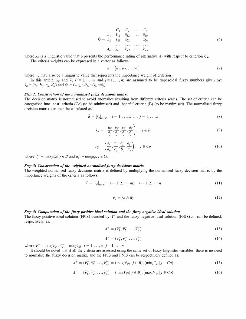
Step 2: Construction of the normalised fuzzy decisions matrix

The decision matrix is normalised to avoid anomalies resulting from different criteria scales. The set of criteria can be

categorised into ‘cost’ criteria (Co) (to be minimised) and ‘benefit’ criteria (B) (to be maximised). The normalised fuzzy

decision matrix can then be calculated as:

~R ¼ ½~rij*m(n; i ¼ 1; . . .;m and j ¼ 1; . . .; n (8)

~rij ¼aij

dþj;bij

dþj;cij

dþj;dij

dþj

!; j 2 B (9)

~rij ¼a&j

dij;a&j

cij;a&j

bij;a&j

aij

& '; j 2 Co (10)

where dþj = max_idijif j ∊ B and a&j = min_iaij, j ∊ Co.

Step 3: Construction of the weighted normalised fuzzy decisions matrix

The weighted normalised fuzzy decisions matrix is defined by multiplying the normalised fuzzy decision matrix by the

importance weights of the criteria as follows:

~V ¼ ½~vij*m(n; i ¼ 1; 2; . . .;m; j ¼ 1; 2; . . .; n (11)

~vij ¼ ~rij ' ~wj (12)

Step 4: Computation of the fuzzy positive ideal solution and the fuzzy negative ideal solution

The fuzzy positive ideal solution (FPIS) denoted by Aþ and the fuzzy negative ideal solution (FNIS) A− can be defined,

respectively, as:

Aþ ¼ ðevþ1 ;evþ2 ; . . .;evþn Þ (13)

A& ¼ ðev&1 ;ev&2 ; . . .;ev&n Þ (14)

where evþj = max_ievij4; ev&j = min_ievij1; i ¼ 1; . . .;m; j = 1, …, n.

It should be noted that if all the criteria are assessed using the same set of fuzzy linguistic variables, there is no need

to normalise the fuzzy decision matrix, and the FPIS and FNIS can be respectively defined as:

Aþ ¼ ðevþ1 ;evþ2 ; . . .;evþn Þ ¼ ðmax_iVij4j j 2 BÞ; ðmin_iVij1j j 2 CoÞ (15)

A& ¼ ðev&1 ;ev&2 ; . . .;ev&n Þ ¼ ðmin_iVij1j j 2 BÞ; ðmax_iVij4j j 2 CoÞ (16)

Step 5: Determination of the distance between each alternative, FPIS and FNIS

The distance from each alternative to the FPIS and the FNIS are:

dþi ¼Xn

j¼1

dðevij;evþj Þ; i ¼ 1; . . .;m (17)

d&i ¼Xn

j¼1

dðevij;ev&j Þ; i ¼ 1; . . .;m (18)

where d(·,·) denotes the distance between two fuzzy numbers, calculated using Equation (5).

Step 6: Computation of the closeness coefficient and ranking the alternatives

In order to aggregate the two distances, a Closeness Coefficient (CC) is calculated for each alternative according to d+

and d− as follows:

CCi ¼d&i

d&i þ dþi; i ¼ 1; . . .;m (19)

CC is defined so that an alternative is close to FPIS and far from FNIS if its closeness coefficient is close to 1.

We shall see in the next section how these methods and tools may be used to address the considered problem.

5. Problem description

The structure of the SC considered in this work is presented in Figure 2. This generic yet simplified SC is composed of

multiple suppliers, multiple parallel manufacturing plants and multiple subcontractors. Each manufacturing plant can

produce several finished products using components provided by the suppliers. Production cost of the same product can

be different according to the manufacturing plant. To increase its production capacity, each manufacturing plant can use

overtime. Regular hours and overtime hours are limited for each period. For simplicity, we have not considered the

transportation costs in this work (they can be considered as included in the costs of products, or can be added in a more

precise way in the models if needed). In addition, it is assumed that the production durations are negligible. Again, tak-

ing into account different production durations complicates the problem without setting specific theoretical issues. Costs

and capacities of each supplier and subcontractor can be different.

We assume that a predefined list of approved suppliers is given. For simplification purpose, it is assumed that a

manufacturing plant is considered as a single stage production system, for instance by considering the bottleneck

resource.

Finished product

Demand

Orders for raw

Materials

Raw material

Raw material

Customers

Parent company

Raw

material

Plants

Production volumes Orders for finished product

Finished product

Finished

product Store

Physical flow Monetary flowInformation flow

Suppliers

Subcontractors

Figure 2. Structure of the supply chain.

6. Proposed approach

6.1 Notation

• Set of indices:

• Crisp parameters:

• Fuzzy parameters:

• Decision variables:

6.2 Presentation of the proposed approach

The suggested approach consists of six main steps.

• Step 1: Select the criteria used for order allocation

In this first step, the decision-maker must choose among Class I and Class II criteria the ones that match with his

strategy, or may add other criteria.

• Step 2: Provide the set of scenarios allowing to satisfy demand requirements

We note:

Cp;t: a set of scenario able to satisfy demand requirements Dp;t

i: index of allocation scenario (i = 1, …, card (Cp;t)) where:

gc rm;p;t Production cost for a unit of product p in regular time at manufacturing plant m in period tgc ovm;p;t Production cost for a unit of product p in overtime at manufacturing plant m in period tgc bb;p;t Subcontracting cost for a unit of product p by subcontractor b in period tgc ss;r;t Purchasing cost of a unit of raw material r at supplier s in period tgQ mm,

gQ bb; gQ ss Linguistic evaluation of quality related, respectively, to manufacturing plant m, to subcontractor b and tosupplier s

gRl mm, gRl bb; gRl ss Linguistic evaluation of the reliability, respectively, related to manufacturing plant m, to subcontractor b andto supplier s

gF mm, gF bb;gF ss Linguistic evaluation of the flexibility related, respectively, to manufacturing plant m, to subcontractor b andto supplier s

gRsp mm,gRsp bb; gRsp ss

Linguistic evaluation of the responsiveness related, respectively, to manufacturing plant m, to subcontractor band to supplier s

gRsi mm,gRsi bb; gRsi ss

Linguistic evaluation of the resilience related, respectively, to manufacturing plant m, to subcontractor b andto supplier s

gRob mm,gRob bb; gRob ss

Linguistic evaluation of the robustness related, respectively, to manufacturing plant m, to subcontractor b andto supplier s

T Number of time periods (t = 1, …, T)P Number of finished products (p = 1, …, P)R Number of raw materials (r = 1, …, R)M Number of manufacturing plants (m = 1 ,…, M)S Number of suppliers (s = 1, …, S)B Number of subcontractors (b = 1, …, B)Sr Set of suppliers providing raw material r (i.e. Sr -{1,…,S})Mp Set of manufacturing plants producing finished product p (i.e. Mp

⊆ {1, …, M})Bp Set of subcontractors supplying finished product p (i.e. Bp -{1, …, B})

Rp Set of raw materials required to produce a final product pαp,r Quantity of raw material r required to produce a unit of final product pcap rm;p;t Maximum number of product p that can be produced in regular time at manufacturing plant m during period tcap ovm;p;t Maximum number of product p that can be produced in overtime at manufacturing plant m during period tcap bb;p;t Maximum number of product p that can be provided by subcontractor b during period tcap ss;r;t Maximum number of raw material r that can be provided by supplier s during period tDp,t Global demand of finished product p in period t resulting from all the customers

x rm;p;t Production quantity in regular time for product p at plant m in period tx ovm;p;t Production quantity in overtime for product p at plant m in period tx bb;p;t Subcontracting quantity for product p at subcontractor b in period tx ss;r;t Purchasing quantity for raw material r from supplier s in period t

Cp;t ¼ fSip;tg ¼ fðx rim;p;tÞm2MP ; ðx ovim;p;tÞm2MP ; ðx bib;p;tÞb2BP ; ðx Si

m;p;tÞm2MP j ð21Þ–ð27Þg (20)

X

m2MP

x rim;p;t þX

m2MP

x ovim;p;t þX

b2BP

x bib;p;t ¼ Dp;t 8i; p; t (21)

X

s2Sr

x sis;r;t ¼ ðX

m2MP

x rim;p;t þX

m2MP

x ovim;p;tÞ ( ap;r 8r 2 Rp; 8i; t (22)

x rim;p;t 1 cap rm;p;t 8i;m; p; t (23)

x ovim;p;t 1 cap ovm;p;t 8i;m; p; t (24)

x bib;p;t 1 cap bb;p;t 8i; b; p; t (25)

x sis;r;t 1 cap ss;r;t 8i; r; s; t (26)

x rim;p;t; x ovim;p;t; x bib;p;t; x sis;r;t 2 0 8i; p; r; t;m; b; s (27)

Constraint (21) ensures that all customer demands are satisfied at the end of each planning period.

The quantity of each raw material to be supplied in each planning period is calculated using constraint (22). Con-

straints (23) and (24) represent the manufacturer’s production capacity limitation during, respectively, regular and over-

time hours.

Constraints (25) and (26) indicate the maximum utilised capacities at each supplier and subcontractor in each period,

respectively.

Constraint (27) expresses the non-negativity of different decision variables.

• Step 3: Evaluate the performance of each allocation scenario

(a) Rate each actor with respect to Class I criteria

The cost is given by a trapezoidal fuzzy number, whereas the quality and the reliability are supposed to be evaluated

by the decision-maker using linguistic labels, according to previous experiences with the partner.

(b) Construct the fuzzy comparison matrix (allocation scenarios-selected criteria of Class I)

Using the results of step 3(a), the fuzzy comparison matrix can be constructed according to the Class I criteria

defined in the first step, using the following proposals:

(i) The cost measure of each allocation scenario is the sum of production costs, supply costs and subcontracting

cots. If fTC ip;t denotes the total cost measure of scenario Sip;t, then:

fTC ip;t ¼

X

m2MP

x rim;p;t 'gc rm;p;t !X

m2MP

x ovim;p;t ' gc ovm;p;t !X

b2BP

x bib;p;t 'gc bb;p;t !

X

s2Sr

X

r2Rp

x sis;r;t 'gc ss;r;t 8i; p; t

(28)

(ii) The measure of each allocation scenario according to the criterion ‘number of actors’ can be evaluated by calcu-

lating the number of manufacturing sites, subcontractors and suppliers involved in this allocation.

If nbip;t denotes the number of actors related of scenario Sip;t then:

nbip;t ¼ cardðEim;p;tÞ 8i; p; t (29)

where

Eim;p;t ¼ fm 2 MPjx rim;p;t[ 0g [ fm 2 MPjx ovim;p;t[ 0g [ fb 2 BPjx bib;p;t[ 0g [ fs 2 Srjx sis;r;t[ 0g (30)

We have now to aggregate the quality and reliability of the suppliers used in each considered scenario. We denote byeQip;t,

eRl ip;t, respectively, the quality and reliability measures associated to allocation scenario Sip;t.

The assessment of each allocation according to the quality (resp. reliability) criterion can be estimated using various

strategies. We limit our discussion to three classical ones, rather intuitive:

• Pessimistic strategy: The quality (resp. reliability) measure associated to an allocation scenario is assumed to be

the quality (resp. reliability) of the worst partner:

~Qip;t ¼ MinðMinm2Ei

m;p;t

gQ mm;p;Minb2Eim;p;t

gQ bb;p;Mins2Eim;p;t

gQ ss;rÞ 8i (31)

eRl ip;t ¼ MinðMinm2Eim;p;t

gRl mm;p;Minb2Eim;p;t

gRl bb;p;Mins2Eim;p;t

gRl ss;rÞ 8i (32)

• Optimistic strategy: The quality (resp. reliability) measure associated to an allocation scenario is assumed to be

the quality (resp. reliability) of the best partner:

eQip;t ¼ Maxð Max

m2Eim;p;t

gQ mm;p; Maxb2Ei

m;p;t

gQ bb;p; Maxs2Ei

m;p;t

gQ ss;rÞ 8i (33)

eRl ip;t ¼ Maxð Maxm2Ei

m;p;t

gRl mm;p; Maxb2Ei

m;p;t

gRl bb;p; Maxb2Ei

m;p;t

gRl ss;rÞ 8i (34)

• Medium strategy: The quality (resp. reliability) measure associated to an allocation scenario is assumed to be the

average of the quality (resp. reliability) measures of the actors involved in this allocation scenario:

~Qip;t ¼

X

m2MP

ðx rim;p;t þ x ovim;p;tÞ 'gQ mm;p

!!

X

b2BP

x bib;p;t 'gQ bb;p

!!

X

s2Sr

X

r2Rp

x sis;r;t 'gQ ss;r

!" #=

X

m2MP

ðx rim;p;t þ x ovim;p;tÞ þX

b2BP

x bib;p;t þX

s2Sr

X

r2Rp

x sis;r;t

!" # (35)

eRl ip;t ¼X

m2MP

ðx rim;p;t þ x ovim;p;tÞ 'eRlm;p

!!

X

b2BP

x bib;p;t 'fRlb;p

!! ðX

s2Sr

X

r2Rp

x sis;r;t 'fRl s;rÞ

" #=

X

m2MP

ðx rim;p;t þ x ovim;p;tÞ þX

b2BP

x bib;p;t þX

s2Sr

X

r2Rp

x sis;r;t

!" # (36)

(c) Use of fuzzy TOPSIS

In this step, we apply the fuzzy TOPSIS method, considering the fuzzy decision matrix described in 3(b) and the

Class I criteria defined in the first step. At the end of this step, we can determine for each allocation scenario Sip;t the

closeness coefficient CC I ip;t.

• Step 4: Evaluate the risk of each allocation scenario

(a) Measure the rating of each actor with respect to Class II criteria

We assume that the decision-maker provides in a linguistic form the rating of each actor with respect to the criteria

of flexibility, responsiveness, resilience and robustness. Concerning the stability criterion, we assume that we have

access to accurate information on the load of the actor during the previous period.

(b) Construct the fuzzy comparison matrix (allocation scenarios-Class II criteria)

The fuzzy decision matrix can be constructed according to the Class II criteria using the result of the previous step

5(a). The rating of each allocation scenario with respect to the criteria of Class II can be calculated according to the

decision-maker strategy (i.e. optimistic strategy, pessimistic strategy or medium strategy) as described previously.

(c) Use of fuzzy TOPSIS

Fuzzy TOPSIS is then used, taking as an input the fuzzy decision matrix obtained in previous step. The method cal-

culates the closeness coefficient of each allocation scenario according to the selected criteria related to Class II. Obvi-

ously, the allocation scenario with the highest closeness coefficient value CC II ip;twill be the less risky.

• Step 5: Interpretation of the results

The use of fuzzy TOPSIS has for outputs the two closeness coefficients related to Class I (performance) and Class

II (risk) criteria. Their interpretation can be facilitated by using rules such as those suggested in Table 1. The perfor-

mance is here rated according to the {do not recommend, recommend, approve} scale, while the risk is denoted by the

{low, moderate, high} linguistic scale. The decision-maker can of course use other linguistic values to rate the allocation

scenarios according to his strategy.

7. Numerical example

In this section, a numerical example is presented to show the applicability of the suggested approach. The main purpose

of this example is to compare in a considered period t the performance and risk of different allocation scenarios that

satisfy the global demand of finished product p Dp;t = 28.

The case study involves two manufacturing plants (m = 1, 2) and two subcontractors (b = 1, 2) who produce the

finished product p. One unit of raw material r is required to produce one unit of p. Each raw material r can be provided

by two suppliers (s = 1, 2). Data on the capacities of the considered SC are given in Table 2.

The decision-maker uses the classical linguistic variables presented in Table 3 to assess the importance of the

various criteria. The linguistic variables shown in Table 4 (also classical) are used to rate the actors with respect to each

criterion (Hatami-Marbini and Tavana 2011).

Table 1. Proposed rules of assessment status of Sip;t .

Closeness coefficient CC I ip;t Closeness coefficient CC II ip;t Assessment status of Sip;t

CC I ip;t 2 [0, 0.4) 8CC II ip;t Do not recommendCC I ip;t 2 [0.4, 0.75) CC II ip;t 2 [0, 0.4) Recommend with high risk

CC II ip;t 2 [0.4, 0.75) Recommend with moderate riskCC II ip;t 2 [0.75, 1] Recommend with low risk

CC I ip;t 2 [0.75, 1] CC II ip;t 2 [0, 0.4) Approved with high riskCC II ip;t 2 [0.4, 0.75) Approved with moderate riskCC II ip;t 2 [0.75, 1] Approved and preferred

Table 2. Capacity data for the supply chain network.

Production capacity in regular time (expressed in term of number of product p) (cap_rm,p,t)m1: 10 m2: 5Production capacity in overtime(expressed in term of number of product p) (cap_ovm,p,t)m1: 5 m2: 5Subcontractor capacity(expressed in term of number of product p) (cap_bb,p,t)b1: 3 b2: 1Supply capacity (expressed in term of number of raw material r) (cap_ss,r,t)s1: 20 s2: 5

The computational procedure can be summarised as follows:

Step 1: Select the used criteria for order allocation

The decision-maker chooses for instance the following criteria:

• Class I: Performance strategy and quality of service

(1) Cost

(2) Quality

(3) Reliability

(4) Number of actors

• Class II: Risk

(1) Flexibility

(2) Responsiveness

(3) Resilience

(4) Robustness

(5) Stability

Step 2: Provide the set of scenario able to satisfy demand requirements

In a preliminary study, the analytical model has been implemented in LINGO in order to get the optimal solution of

the problem when a simple objective function linked to cost is used (Khemiri et al. 2015). As a consequence, reusing

the LINGO model while removing the objective function allows easily generating all the possible scenarios satisfying

the demand (see Table 5); the solver was therefore used for checking the satisfaction of the constraints.

Step 3: Evaluate the performance of each allocation scenario

• Assess the rating of each actor with respect to Class I criteria

The ratings of the actors defined by the decision-maker according to the various criteria of Class I are shown in

Table 6. The cost ratings are given as trapezoidal fuzzy numbers while the quality and reliability ratings are given

through linguistic variables that can be converted into trapezoidal fuzzy numbers using Table 4.

• Construct the fuzzy comparison matrix

We assume that the decision-maker uses the medium strategy to assess each allocation scenario on the quality and

reliability criteria (formulae (35) and (36)). The cost measures are obtained using formula (28) and the number of actors

is given by formula (29). The result is the fuzzy decision matrix of Table 7.

Table 3. Linguistic variables for the importance weight of each criterion (Hatami-Marbini and Tavana 2011).

Very low (VL) (0; 0; 0.1; 0.2)Low (L) (0.1; 0.2; 0.2; 0.3)Medium low (ML) (0.2; 0.3; 0.4; 0.5)Medium (M) (0.4; 0.5; 0.5; 0.6)Medium high (MH) (0.5; 0.6; 0.7; 0.8)High (H) (0.7; 0.8; 0.8; 0.9)Very high (VH) (0.8; 0.9; 1.0; 1.0)

Table 4. Linguistic variables for ratings (Hatami-Marbini and Tavana 2011).

Very poor (VP) (0; 0; 1; 2)Poor (P) (1; 2; 2; 3)Medium poor (MP) (2; 3; 4; 5)Fair (F) (4; 5; 5; 6)Medium good (MG) (5; 6; 7; 8)Good (G) (7; 8; 8; 9)Very good (VG) (8; 9; 10; 10)

• Use of Fuzzy TOPSIS

Fuzzy TOPSIS is used with as input the fuzzy decision matrix shown in Table 7. The importance weights of the

Class I criteria determined by the decision-maker are shown in Table 8. Table 7 is used to obtain the normalised Fuzzy

decision matrix presented in Table 9 using the formulae (9) and (10). Using the normalised Fuzzy decision matrix and

the importance weights of the criteria in Table 8, a weight normalised Fuzzy decision matrix is calculated using formula

(12), as shown in Table 10.

Table 5. The set of allocation scenarios.

Allocation scenarios

Quantity

x_rm1,p,t x_rm2,p,t x_ovm1,p,t x_ovm2,p,t x_bb1,p,t x_bb2,p,t x_ss1,r,t x_ss2,r,t

S1p;t 10 5 5 5 3 0 20 5

S2p;t 9 5 5 5 3 1 19 5

S3p;t 9 5 5 5 3 1 20 4

S4p;t 10 4 5 5 3 1 19 5

S5p;t 10 4 5 5 3 1 20 4

S6p;t 10 5 4 5 3 1 19 5

S7p;t 10 5 4 5 3 1 20 4

S8p;t 10 5 5 4 3 1 19 5

S9p;t 10 5 5 4 3 1 20 4

S10p;t 10 5 5 5 2 1 20 5

Table 6. Ratings of the actors by the decision-maker using selected criteria of Class I.

Criteria Class I

Actors

m1 m2 b1 b2 s1 s2

Cost Regular time cost: Regular time cost: (45, 50, 50, 53) (250,260,265,270) (5,10,12,17) (10,15,20,25)(9, 10, 11, 12) (1, 2, 3, 5)Overtime cost: Overtime cost:(26, 27,28,30) (15, 16, 17, 20)

Quality G VG MG P G VGReliability G VG G VP MG VG

Table 7. Fuzzy comparison matrix (allocation scenarios-Class I criteria).


Criteria

Cost Quality Reliability Number of actors

S1p;t (585, 750, 840, 1019) (7.169, 8.169,8.509,9.226) (6.528,7.528, 8.188, 8.905) (5,5,5,5)

S2p;t (821, 990, 1082,1260) (7.057,8.057, 8.403, 9.115) (6.423,7.403, 8.076, 8.788) (6,6,6,6)

S3p;t (816, 985, 1074,1252) (7.038,8.038, 8.365, 9.096) (6.365,7.346, 8.019, 8.750) (6,6,6,6)

S4p;t (829, 998, 1090,1267) (7.038,8.038, 8.365, 9.096) (6.403,7.384, 8.038, 8.769) (6,6,6,6)

S5p;t (824, 993, 1082,1259) (7.019,8.019, 8.326, 9.076) (6.346,7.326, 7.980, 8.730) (6,6,6,6)

S6p;t (804, 973, 1065,1242) (7.057,8.057, 8.403, 9.115) (6.423,7.403, 8.076, 8.788) (6,6,6,6)

S7p;t (799, 968, 1057,1234) (7.038,8.038, 8.365, 9.096) (6.365,7.346, 8.019, 8.750) (6,6,6,6)

S8p;t (815, 984, 1076,1252) (7.038,8.038, 8.365, 9.096) (6.403,7.384, 8.038, 8.769) (6,6,6,6)

S9p;t (810, 979, 1068,1244) (7.019,8.019, 8.326, 9.076) (6.346,7.326, 7.980, 8.730) (6,6,6,6)

S10p;t (790, 960, 1055,1236) (7.094,8.094, 8.415, 9.132) (6.396,7.377, 8.056, 8.773) (6,6,6,6)

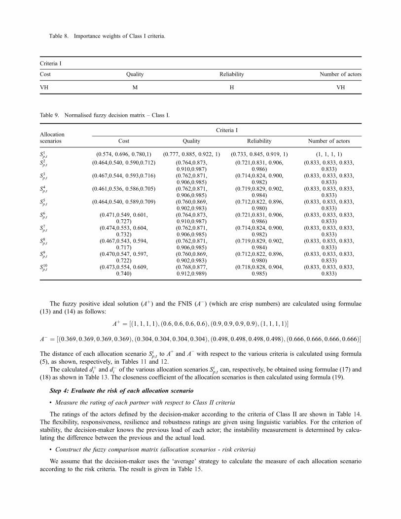
The fuzzy positive ideal solution (Aþ) and the FNIS (A&) (which are crisp numbers) are calculated using formulae

(13) and (14) as follows:

Aþ ¼ ½ð1; 1; 1; 1Þ; ð0:6; 0:6; 0:6; 0:6Þ; ð0:9; 0:9; 0:9; 0:9Þ; ð1; 1; 1; 1Þ*

A& ¼ ½ð0:369; 0:369; 0:369; 0:369Þ; ð0:304; 0:304; 0:304; 0:304Þ; ð0:498; 0:498; 0:498; 0:498Þ; ð0:666; 0:666; 0:666; 0:666Þ*

The distance of each allocation scenario Sip;t to A+ and A− with respect to the various criteria is calculated using formula

(5), as shown, respectively, in Tables 11 and 12.

The calculated dþi and d&i of the various allocation scenarios Sip;t can, respectively, be obtained using formulae (17) and

(18) as shown in Table 13. The closeness coefficient of the allocation scenarios is then calculated using formula (19).

Step 4: Evaluate the risk of each allocation scenario

• Measure the rating of each partner with respect to Class II criteria

The ratings of the actors defined by the decision-maker according to the criteria of Class II are shown in Table 14.

The flexibility, responsiveness, resilience and robustness ratings are given using linguistic variables. For the criterion of

stability, the decision-maker knows the previous load of each actor; the instability measurement is determined by calcu-

lating the difference between the previous and the actual load.

• Construct the fuzzy comparison matrix (allocation scenarios - risk criteria)

We assume that the decision-maker uses the ‘average’ strategy to calculate the measure of each allocation scenario

according to the risk criteria. The result is given in Table 15.

rch Table 8. Importance weights of Class I criteria.

Criteria I


VH M H VH

Table 9. Normalised fuzzy decision matrix – Class I.

Allocationscenarios

Criteria I


S1p;t (0.574, 0.696, 0.780,1) (0.777, 0.885, 0.922, 1) (0.733, 0.845, 0.919, 1) (1, 1, 1, 1)

S2p;t (0.464,0.540, 0.590,0.712) (0.764,0.873,0.910,0.987)

(0.721,0.831, 0.906,0.986)

(0.833, 0.833, 0.833,0.833)

S3p;t (0.467,0.544, 0.593,0.716) (0.762,0.871,0.906,0.985)

(0.714,0.824, 0.900,0.982)

(0.833, 0.833, 0.833,0.833)

S4p;t (0.461,0.536, 0.586,0.705) (0.762,0.871,0.906,0.985)

(0.719,0.829, 0.902,0.984)

(0.833, 0.833, 0.833,0.833)

S5p;t (0.464,0.540, 0.589,0.709) (0.760,0.869,0.902,0.983)

(0.712,0.822, 0.896,0.980)

(0.833, 0.833, 0.833,0.833)

S6p;t (0.471,0.549, 0.601,0.727)

(0.764,0.873,0.910,0.987)

(0.721,0.831, 0.906,0.986)

(0.833, 0.833, 0.833,0.833)

S7p;t (0.474,0.553, 0.604,0.732)

(0.762,0.871,0.906,0.985)

(0.714,0.824, 0.900,0.982)

(0.833, 0.833, 0.833,0.833)

S8p;t (0.467,0.543, 0.594,0.717)

(0.762,0.871,0.906,0.985)

(0.719,0.829, 0.902,0.984)

(0.833, 0.833, 0.833,0.833)

S9p;t (0.470,0.547, 0.597,0.722)

(0.760,0.869,0.902,0.983)

(0.712,0.822, 0.896,0.980)

(0.833, 0.833, 0.833,0.833)

S10p;t (0.473,0.554, 0.609,0.740)

(0.768,0.877,0.912,0.989)

(0.718,0.828, 0.904,0.985)

(0.833, 0.833, 0.833,0.833)

Table 10. Weighted normalised fuzzy decision matrix – Class I

AllocationScenarios

Criteria


S1p;t (0.459, 0.626, 0.780, 1) (0.310, 0.442, 0.461, 0.6) (0.513, 0.676, 0.735, 0.9) (0.8, 0.9, 1, 1)

S2p;t (0.371, 0.486, 0.590,0.712)

(0.305, 0.436, 0.455,0.592)

(0.504, 0.665, 0.725,0.888)

(0.666, 0.750, 0.833,0.833)

S3p;t (0.373, 0.490, 0.593,0.716)

(0.305, 0.435, 0.453,0.591)

(0.500, 0.659, 0.720,0.884)

(0.666, 0.750, 0.833,0.833)

S4p;t (0.369, 0.483, 0.586,0.705)

(0.305, 0.435, 0.453,0.591)

(0.503, 0.663, 0.722,0.886)

(0.666, 0.750, 0.833,0.833)

S5p;t (0.371, 0.486, 0.589,0.709)

(0.304, 0.434, 0.451,0.590)

(0.498, 0.658, 0.716,0.882)

(0.666, 0.750, 0.833,0.833)

S6p;t (0.376, 0.494, 0.601,0.727)

(0.305, 0.436, 0.455,0.592)

(0.504, 0.665, 0.725,0.888)

(0.666, 0.750, 0.833,0.833)

S7p;t (0.379, 0.498, 0.604,0.732)

(0.305, 0.435, 0.453,0.591)

(0.500, 0.659, 0.720,0.884)

(0.666, 0.750, 0.833,0.833)

S8p;t (0.373, 0.489, 0.594,0.717)

(0.305, 0.435, 0.453,0.591)

(0.503, 0.663, 0.722,0.886)

(0.666, 0.750, 0.833,0.833)

S9p;t (0.376, 0.492, 0.597,0.722)

(0.304, 0.434, 0.451,0.590)

(0.498, 0.658, 0.716,0.882)

(0.666, 0.750, 0.833,0.833)

S10p;t (0.378, 0.499, 0.609,0.740)

(0.307, 0.438, 0.456,0.593)

(0.502, 0.662, 0.723,0.886)

(0.666, 0.750, 0.833,0.833)

Table 11. Distance between each allocation scenario and Aþ.


Criteria


S1p;t 0.3464 0.1786 0.2380 0.1118S2p;t 0.4766 0.1830 0.2459 0.2393S3p;t 0.4735 0.1840 0.2499 0.2393S4p;t 0.4803 0.1840 0.2475 0.2393S5p;t 0.4772 0.1850 0.2516 0.2393S6p;t 0.4683 0.1830 0.2459 0.2393S7p;t 0.4651 0.1840 0.2499 0.2393S8p;t 0.4735 0.1840 0.2475 0.2393S9p;t 0.4704 0.1850 0.2516 0.2393S10p;t 0.4628 0.1818 0.2476 0.2393

Figure 3. The performance and risk of the allocation scenarios.

• Use of fuzzy TOPSIS

• The decision-maker provides the weights of the risk criteria shown in Table 16. This table and the fuzzy decision

matrix presented in Table 15 are used for calculating the closeness coefficient for each allocation scenario as

shown in Table 17.

Step 5: Interpretation of the results

The rules presented in Table 1 have been used to classify the allocation scenarios in Figure 3. As seen in Figure 3, the

first scenario S1p;t denotes better performance and risk measures than the other solutions, and is ‘recommended’ with

rch Table 12. Distance between each allocation scenario and A&.


Criteria


S1p;t 0.4001 0.1811 0.2493 0.2713

S2p;t 0.2124 0.1757 0.2401 0.1250

S3p;t 0.2155 0.1746 0.2364 0.1250

S4p;t 0.2079 0.1746 0.2382 0.1250

S5p;t 0.2109 0.1734 0.2345 0.1250

S6p;t 0.2223 0.1757 0.2401 0.1250

S7p;t 0.2255 0.1746 0.2364 0.1250

S8p;t 0.2159 0.1746 0.2382 0.1250

S9p;t 0.2190 0.1734 0.2345 0.1250

S10p;t 0.2303 0.1767 0.2386 0.1250

Table 13. Computation of dþip;t , d

&i;jp;t and CC I ip;t .

Allocation scenarios dþip;t d&i

p;t CC I ip;t

S1p;t 0.8749 1.1019 0.5574

S2p;t 1.1449 0.7533 0.3968

S3p;t 1.1469 0.7515 0.3958

S4p;t 1.1513 0.7458 0.3931

S5p;t 1.1533 0.7439 0.3921

S6p;t 1.1366 0.7632 0.4017

S7p;t 1.1385 0.7615 0.4008

S8p;t 1.1445 0.7537 0.3970

S9p;t 1.1465 0.7520 0.3961

S10p;t 1.1317 0.7707 0.4051

Table 14. Ratings of the actors by the decision-maker under Class II criteria.

Criteria Class B

Actors

m1 m2 b1 b2 s1 s2

Flexibility VG MG VG VP MG GResponsiveness VG G VG VP VG GResilience VG G VG VP VG VGRobustness G VG VG VP VG MGStability (Previous load) x rm1;p;t&1 ¼ 11 x rm2;p;t&1 ¼ 5 3 0 20 5

x ovm1;p;t&1 ¼ 5 x ovm2;p;t&1 ¼ 5

Table 15. Fuzzy comparison matrix (allocation scenarios-Class II criteria).


Risk criteria

Flexibility Responsiveness Resilience Robustness Stability

S1p;t (6.207,7.207,8.113,8.773) (7.716,8.716,9.433,9.716) (7.811,8.811,9.622,9.811) (7.433,8.433,9.150,9.528) (0.125,0.125,0.125,0.125)

S2p;t (6.076,7.057,7.961,8.634) (7.557,8.538,9.250,9.557) (7.653,8.634,9.442,9.653) (7.288,8.269,9.000,9.384) (0.5,0.5,0.5,0.5)

S3p;t (6.038,7.019,7.942,8.615) (7.576,8.557,9.288,9.576) (7.653,8.634,9.442,9.653) (7.346,8.326,9.057,9.423) (0.5,0.5,0.5,0.5)

S4p;t (6.134,7.115,8.019,8.673) (7.576,8.557,9.288,9.576) (7.673,8.653,9.480,9.673) (7.269,8.250,8.961,9.365) (0.5,0.5,0.5,0.5)

S5p;t (6.096,7.076,8.000,8.653) (7.596,8.576,9.326,9.596) (7.673,8.653,9.480,9.673) (7.326,8.307,9.019,9.403) (0.5,0.5,0.5,0.5)

S6p;t (6.076,7.057,7.961,8.634) (7.557,8.538,9.250,9.557) (7.653,8.634,9.442,9.653) (7.288,8.269,9.000,9.384) (0.5,0.5,0.5,0.5)

S7p;t (6.038,7.019,7.942,8.615) (7.576,8.557,9.288,9.576) (7.653,8.634,9.442,9.653) (7.346,8.326,9.057,9.423) (0.5,0.5,0.5,0.5)

S8p;t (6.134,7.115,8.019,8.673) (7.576,8.557,9.288,9.576) (7.673,8.653,9.480,9.673) (7.269,8.250,8.961,9.365) (0.5,0.5,0.5,0.5)

S9p;t (6.096,7.076,8.000,8.653) (7.596,8.576,9.326,9.596) (7.673,8.653,9.480,9.673) (7.326,8.307,9.019,9.403) (0.5,0.5,0.5,0.5)

S10p;t (6.056,7.037,7.943,8.622) (7.566,8.547,9.264,9.566) (7.660,8.641,9.452,9.660) (7.283,8.264,8.981,9.377) (0.375,0.375,0.375,0.375)

rch Table 16. Importance weights of Class II criteria.

Criteria B

Flexibility Responsiveness Resilience Robustness Stability

VH H H VH VH

Table 17. Computation of CC II ip;t .

Allocation scenarios CC II ip;t

S1p;t 0.6367

S2p;t 0.3679

S3p;t 0.3692

S4p;t 0.3700

S5p;t 0.3713

S6p;t 0.3679

S7p;t 0.3692

S8p;t 0.3700

S9p;t 0.3713

S10p;t 0.3950

Table 18. Experiments for sensibility analysis.

Expt. no.

Definition

Importance weights of Class I criteria Importance weights of Class II criteria

Cost Quality Reliability Number of actors Flexibility Responsiveness Resilience Robustness Stability

1 VL VL VL VL VL VL VL VL VL2 M M M M M M M M M3 VH VH VH VH VH VH VH VH VH4 VH VL VL VL VL VL VL VL VL5 VL VH VL VL VL VL VL VL VL6 VL VL VH VL VL VL VL VL VL7 VL VL VL VH VL VL VL VL VL8 VL VL VL VL VH VL VL VL VL9 VL VL VL VL VL VH VL VL VL10 VL VL VL VL VL VL VH VL VL11 VL VL VL VL VL VL VL VH VL12 VL VL VL VL VL VL VL VL VH13 VH VH VH VH VL VL VL VL VL14 VL VL VL VL VH VH VH VH VH15 VL L ML M MH H VH VH VL16 VH H MH M ML L VL VL VH17 H ML M MH L VL VH H ML18 ML MH VH VL L M H H M

Table 19. Results of sensibility analysis: performance measure.

Expt.no.

CC I ip;t

RankingR1 R2 R3 R4 R5 R6 R7 R8 R9 R10

1 0.4199 0.3856 0.3854 0.3847 0.3844 0.3867 0.3865 0.3856 0.3854 0.3877 R1>R10>R6>R7>R8>R2>R9>R3>R4>R52 0.5203 0.4051 0.4039 0.4020 0.4008 0.4085 0.4073 0.4048 0.4036 0.4112 R1>R10>R6>R7>R2>R8>R3>R9>R4>R53 0.5729 0.4240 0.4224 0.4200 0.4183 0.4284 0.4269 0.4236 0.4220 0.4318 R1>R10>R6>R7>R2>R8>R3>R9>R4>R54 0.4781 0.3590 0.3607 0.3558 0.3575 0.3654 0.3672 0.3610 0.3627 0.3702 R1>R10>R7>R6>R9>R8>R3>R2>R5>R45 0.4699 0.4369 0.4352 0.4347 0.4330 0.4378 0.4361 0.4354 0.4338 0.4400 R1>R10>R6>R2>R7>R8>R3>R4>R9>R56 0.4714 0.4393 0.4359 0.4371 0.4337 0.4401 0.4368 0.4378 0.4344 0.4395 R1>R6>R10>R2>R8>R4>R7>R3>R9>R57 0.5129 0.3736 0.3734 0.3728 0.3726 0.3747 0.3745 0.3736 0.3734 0.3756 R1>R10>R6>R7>R8>R2>R9>R3>R4>R58 0.4199 0.3856 0.3854 0.3847 0.3844 0.3867 0.3865 0.3856 0.3854 0.3877 R1>R10>R6>R7>R8>R2>R9>R3>R4>R59 0.4199 0.3856 0.3854 0.3847 0.3844 0.3867 0.3865 0.3856 0.3854 0.3877 R1>R10>R6>R7>R8>R2>R9>R3>R4>R510 0.4199 0.3856 0.3854 0.3847 0.3844 0.3867 0.3865 0.3856 0.3854 0.3877 R1>R10>R6>R7>R8>R2>R9>R3>R4>R511 0.4199 0.3856 0.3854 0.3847 0.3844 0.3867 0.3865 0.3856 0.3854 0.3877 R1>R10>R6>R7>R8>R2>R9>R3>R4>R512 0.4199 0.3856 0.3854 0.3847 0.3844 0.3867 0.3865 0.3856 0.3854 0.3877 R1>R10>R6>R7>R8>R2>R9>R3>R4>R513 0.5729 0.4240 0.4224 0.4200 0.4183 0.4284 0.4269 0.4236 0.4220 0.4318 R1>R10>R6>R7>R2>R8>R3>R9>R4>R514 0.4199 0.3856 0.3854 0.3847 0.3844 0.3867 0.3865 0.3856 0.3854 0.3877 R1>R10>R6>R7>R8>R2>R9>R3>R4>R515 0.4999 0.4208 0.4194 0.4194 0.4180 0.4217 0.4203 0.4201 0.4187 0.4223 R1>R10>R6>R2>R7>R8>R3>R4>R9>R516 0.5304 0.4058 0.4049 0.4021 0.4011 0.4105 0.4097 0.4059 0.4050 0.4142 R1>R10>R6>R7>R8>R2>R9>R3>R4>R517 0.5215 0.3925 0.3922 0.3896 0.3892 0.3968 0.3966 0.3930 0.3928 0.3999 R1>R10>R6>R7>R8>R9>R2>R3>R4>R518 0.4984 0.4459 0.4433 0.4430 0.4403 0.4481 0.4455 0.4447 0.4421 0.4495 R1>R10>R6>R2>R7>R8>R3>R4>R9>R5

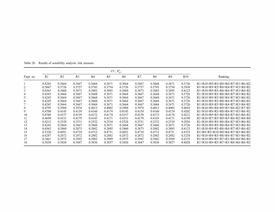
Table 20. Results of sensibility analysis: risk measure.

Expt. no.

CC II ip;t

RankingR1 R2 R3 R4 R5 R6 R7 R8 R9 R10

1 0.4245 0.3664 0.3667 0.3668 0.3671 0.3664 0.3667 0.3668 0.3671 0.3726 R1>R10>R9>R5>R8>R4>R7>R3>R6>R22 0.5847 0.3726 0.3737 0.3743 0.3754 0.3726 0.3737 0.3743 0.3754 0.3930 R1>R10>R9>R5>R8>R4>R7>R3>R6>R23 0.6565 0.3860 0.3873 0.3882 0.3895 0.3860 0.3873 0.3882 0.3895 0.4123 R1>R10>R9>R5>R8>R4>R7>R3>R6>R24 0.4245 0.3664 0.3667 0.3668 0.3671 0.3664 0.3667 0.3668 0.3671 0.3726 R1>R10>R9>R5>R8>R4>R7>R3>R6>R25 0.4245 0.3664 0.3667 0.3668 0.3671 0.3664 0.3667 0.3668 0.3671 0.3726 R1>R10>R9>R5>R8>R4>R7>R3>R6>R26 0.4245 0.3664 0.3667 0.3668 0.3671 0.3664 0.3667 0.3668 0.3671 0.3726 R1>R10>R9>R5>R8>R4>R7>R3>R6>R27 0.4245 0.3664 0.3667 0.3668 0.3671 0.3664 0.3667 0.3668 0.3671 0.3726 R1>R10>R9>R5>R8>R4>R7>R3>R6>R28 0.4795 0.3984 0.3974 0.4013 0.4002 0.3984 0.3974 0.4013 0.4002 0.4024 R1>R10>R8>R4>R9>R5>R6>R2>R7>R39 0.4700 0.4145 0.4159 0.4160 0.4174 0.4145 0.4159 0.4160 0.4174 0.4202 R1>R10>R9>R5>R8>R4>R7>R3>R6>R210 0.4709 0.4157 0.4159 0.4172 0.4174 0.4157 0.4159 0.4172 0.4174 0.4212 R1>R10>R9>R5>R8>R4>R7>R3>R6>R211 0.4694 0.4151 0.4179 0.4143 0.4171 0.4151 0.4179 0.4143 0.4171 0.4198 R1>R10>R7>R3>R9>R5>R6>R2>R8>R412 0.6215 0.2528 0.2531 0.2532 0.2534 0.2528 0.2531 0.2532 0.2534 0.2936 R1<R10<R9<R5<R8<R4<R7<R3<R6<R213 0.4245 0.3664 0.3667 0.3668 0.3671 0.3664 0.3667 0.3668 0.3671 0.3726 R1>R10>R9>R5>R8>R4>R7>R3>R6>R214 0.6565 0.3860 0.3873 0.3882 0.3895 0.3860 0.3873 0.3882 0.3895 0.4123 R1>R10>R9>R5>R8>R4>R7>R3>R6>R215 0.5320 0.4691 0.4710 0.4712 0.4731 0.4691 0.4710 0.4712 0.4731 0.4723 R1>R9>R5>R10>R8>R4>R7>R3>R6>R216 0.6287 0.2872 0.2872 0.2882 0.2882 0.2872 0.2872 0.2882 0.2882 0.3238 R1>R10>R9>R5>R8>R4>R7>R3>R6>R217 0.5461 0.3975 0.3992 0.3982 0.3999 0.3975 0.3992 0.3982 0.3999 0.4125 R1>R10>R9>R5>R7>R3>R8>R4>R6>R218 0.5838 0.3826 0.3847 0.3836 0.3857 0.3826 0.3847 0.3836 0.3857 0.4028 R1>R10>R9>R5>R7>R3>R8>R4>R6>R2

‘moderate risk’. The main reason is that this scenario implies fewer actors (5 actors instead of 6 in the other scenarios);

moreover, subcontractor b2, who has a poor performance (high cost, poor quality and reliability) and a very low resis-

tance to the risk factors (very poor flexibility, responsiveness, etc.) is not involved.

The scenarios S6p;t, S7p;t and S10p;t are recommended with high risk whereas all the other scenarios are not recom-

mended according to the rules suggested in Table 1.

In our opinion, the results presented in Figure 3 may allow a decision-maker to determine a balanced solution

between expected performance and risk.

8. Sensitivity analysis

The use of overlapping fuzzy weights is known as giving some intrinsic robustness to the aggregation method. As an

illustration, a sensitivity analysis was conducted. The details of 18 experiments are summarised in Table 18. For exam-

ple, in the first three experiments, the weights of all decision criteria are assumed to be equal to ‘VL’, ‘M’ and ‘VH’. In

experiments 4–12, the importance weight of each decision criteria is assumed to be ‘Very High (VH)’ and the rest of

the criteria are set to ‘Very Low (VL)’. In experiment 13 (resp. 14), the weights of all performance-based decision

criteria (resp. risk-based decision criteria) are set to the highest value (VH), while weights of all risk-based decision cri-

teria (resp. performance-based decision criteria) are set as lowest value (VL). The remaining experiments were randomly

generated.

The results of the sensitivity analysis are illustrated in Tables 19 and 20. It can be seen that, although the rank of

some allocation scenarios changes with respect to different fuzzy weight bases, S1p;t is still selected as the best allocation

scenario, since it has the highest performance and risk measures. We can also notice that out of 18 experiments, S10p;t has

the second rank in 17 experiments according to both performance and risk measures. Additionally, the allocation sce-

nario S5p;t has the lowest performance score in all the experiments and S2p;t has the lowest risk score in 16 experiments.

Therefore, we can conclude that the proposed decision-making approach is relatively robust to small changes in the

fuzzy criteria weights on this example.

9. Conclusion and future research work

Nowadays, most SC networks are affected by various sources of uncertainty, including an increased variability of the

demand. Consequently, making explicit the risk linked to the future execution of a supply plan may be an asset for sup-

porting the decision of the logistic managers. However, the academic literature still shows a lack of approaches consid-

ering risk-based factors when constructing a procurement–production tactical plan. The existing studies are indeed

mainly based on the optimisation of performance factors, and often focus on price or profit criteria.

This article proposes to use a multi-criteria decision-making approach to deal with an integrated procurement–

production system in a multi-echelon SC network involving multiple suppliers, multiple production sites, multiple sub-

contractors and several customers, in which some critical data are evaluated in an imprecise way using fuzzy logic. The

decision-maker selects first risk-based and performance-based decision criteria that match his strategy and his industrial

context. The set of possible plans is generated as well as their performance and risk measures, in order to better support

the selection of a procurement–production plan.

The main interest of the proposal is in our opinion to keep a clear distinction between assessment criteria linked to

performance and to risk, since there is clearly no ‘mechanical’ compensation between these types of criteria in real situ-

ations

Another interest of the method is that it better preserves the decision maker’s preferences than existing optimisation

approaches. Additionally, it provides appropriate flexibility to the decision-maker for selecting the preferred tactical plan

among several alternatives. The developed approach is generic in nature and can be easily extended to other selection

problems.

The suggested approach has of course limitations. Some of them are classical, like the possible interaction between

the dispersion of the assessments and the weights of the criteria. Others are linked to the chosen strategy, i.e. the genera-

tion of all the possible scenarios, which makes difficult to address very large/multi-period problems. Extensions of this

work are in progress for defining heuristics in order to only generate a given number of ‘good’ scenarios. Other limita-

tions are linked to the hypothesis considered for simplifying the problem: it would for instance be more realistic to

incorporate several distribution centres in order to deal with an integrated procurement, production and distribution plan-

ning problem. The method should also be extended to take into account the various lead times associated with purchas-

ing and manufacturing. Additionally, we assumed for simplicity that the customer demand is deterministic: it would be

interesting to consider it as uncertain. Addressing these limitations will be the next step of this study.

Disclosure statement

No potential conflict of interest was reported by the authors.

References

Arabzad, S. M., M. Ghorbani, J. Razmi, and H. Shirouyehzad. 2015. “Employing Fuzzy TOPSIS and SWOT for Supplier Selection

and Order Allocation Problem.” The International Journal of Advanced Manufacturing Technology 76 (5–8): 803–818.

Baumann, P., and N. Trautmann. 2013. “A Continuous-time MILP Model for Short-term Scheduling of Make-and-pack Production

Processes.” International Journal of Production Research 51 (6): 1707–1727.

Bellman, R. E., and L. A. Zadeh. 1970. “Decision-making in a Fuzzy Environment.” Management Science 17 (4): B-141.

Bhamra, R., S. Dani, and K. Burnard. 2011. “Resilience: The Concept, a Literature Review and Future Directions.” International

Journal of Production Research 49 (18): 5375–5393.

Brans, J., and P. Vincke. 1985. “A Preference Ranking Organisation Method: The PROMETHEE Method for MCDM.” Management

Science 31 (6): 647–656.

Buckley, J. J. 1985. “Fuzzy Hierarchical Analysis.” Fuzzy Sets and Systems 17 (3): 233–247.

Chauhan, S. S., R. Nagi, and J. M. Proth. 2004. “Strategic Capacity Planning in Supply Chain Design for a New Market Opportu-

nity.” International Journal of Production Research 42 (11): 2197–2206.

Chen, C. T. 2000. “Extensions of the TOPSIS for Group Decision-making under Fuzzy Environment.” Fuzzy Sets and Systems

114 (1): 1–9.

Chen, S. P., and P. C. Chang. 2006. “A Mathematical Programming Approach to Supply Chain Models with Fuzzy Parameters.”

Engineering Optimization 38 (6): 647–669.

Chen, S. P., and W. L. Huang. 2010. “A Membership Function Approach for Aggregate Production Planning Problems in Fuzzy

Environments.” International Journal of Production Research 48 (23): 7003–7023.

Chen, C. T., C. T. Lin, and S. F. Huang. 2006. “A Fuzzy Approach for Supplier Evaluation and Selection in Supply Chain Manage-

ment.” International Journal of Production Economics 102 (2): 289–301.

Chhaochhria, P., and S. C. Graves. 2013. “A Forecast-driven Tactical Planning Model for a Serial Manufacturing System.” Interna-

tional Journal of Production Research 51 (23–24): 6860–6879.

Chou, S. Y., Y. H. Chang, and C. Y. Shen. 2008. “A Fuzzy Simple Additive Weighting System under Group Decision-making

for Facility Location Selection with Objective/Subjective Attributes.” European Journal of Operational Research 189 (1):

132–145.

Curcurù, G., G. M. Galante, and C. M. La Fata. 2013. “An Imprecise Fault Tree Analysis for the Estimation of the Rate Of OCcur-

rence of Failure (ROCOF).” Journal of Loss Prevention in the Process Industries 26 (6): 1285–1292.

Cyrulnik, B., and D. Macey. 2009. Resilience: How Your Inner Strength Can Set You Free from the past. London: Penguin Books.

Dickson, G. W. 1966. “An Analysis of Supplier Selection Systems and Decision.” Journal of Purchasing and Materials Management

2: 5–17.

Ellram, L. 1990. “The Supplier Selection Decision in Strategic Partnerships.” Journal of Purchasing and Material Management

26 (1): 8–14.

Genin, P., S. Lamouri, and A. Thomas. 2008. “Multi-facilities Tactical Planning Robustness with Experimental Design.” Production

Planning and Control 19 (2): 171–182.

Gholamian, N., I. Mahdavi, and R. Tavakkoli-Moghaddam. 2016. “Multi-objective Multi-product Multi-site Aggregate Production

Planning in a Supply Chain under Uncertainty: Fuzzy Multi-objective Optimisation.” International Journal of Computer Inte-

grated Manufacturing 29 (2): 149–165.

Gholamian, N., I. Mahdavi, R. Tavakkoli-Moghaddam, and N. Mahdavi-Amiri. 2015. “Comprehensive Fuzzy Multi-objective Multi-

product Multi-site Aggregate Production Planning Decisions in a Supply Chain under Uncertainty.” Applied Soft Computing

37: 585–607.

Gigović, L., D. Pamučar, Z. Bajić, and M. Milićević. 2016. “The Combination of Expert Judgment and GIS-MAIRCA Analysis for

the Selection of Sites for Ammunition Depot.” Sustainability 8, 372.

Gigović, L., D. Pamučar, D. Božanić, and S. Ljubojević. 2017. “Application of the GIS-DANP-MABAC Multi-criteria Model for

Selecting the Location of Wind Farms: A Case Study of Vojvodina, Serbia.” Renewable Energy 103: 501–521.

Giri, B. C., S. Bardhan, and T. Maiti. 2016. “Coordinating a Three-layer Supply Chain with Uncertain Demand and Random Yield.”

International Journal of Production Research 54 (8): 2499–2518.

Goffin, K., M. Szwejczewski, and C. New. 1997. “Managing Suppliers: When Fewer Can Mean More.” International Journal of

Physical Distribution & Logistics Management 27 (7): 422–436.

Goyal, S. K., and S. G. Deshmukh. 1992. “Integrated Procurement–Production Systems: A Review.” European Journal of Opera-

tional Research 62 (1): 1–10.

Guneri, A. F., A. Yucel, and G. Ayyildiz. 2009. “An Integrated Fuzzy-lp Approach for a Supplier Selection Problem in Supply Chain

Management.” Expert Systems with Applications 36 (5): 9223–9228.

Gupta, A., and C. D. Maranas. 1999. “A Hierarchical Lagrangean Relaxation Procedure for Solving Midterm Planning Problems.”

Industrial & Engineering Chemistry Research 38 (5): 1937–1947.

Gupta, A., and C. D. Maranas. 2003. “Managing Demand Uncertainty in Supply Chain Planning.” Computers and Chemical

Engineering 27 (8–9): 1219–1227.

Haldar, A., A. Ray, D. Banerjee, and S. Ghosh. 2012. “A Hybrid MCDM Model for Resilient Supplier Selection.” International

Journal of Management Science and Engineering Management 7 (4): 284–292.

Haldar, A., A. Ray, D. Banerjee, and S. Ghosh. 2014. “Resilient Supplier Selection under a Fuzzy Environment.” International

Journal of Management Science and Engineering Management 9 (2): 147–156.

Hatami-Marbini, A., and M. Tavana. 2011. “An Extension of the Electre I Method for Group Decision-making under a Fuzzy Envi-

ronment.” Omega. 39: 373–386.

Huang, S. H., and H. Keskar. 2007. “Comprehensive and Configurable Metrics for Supplier Selection.” International Journal of Pro-

duction Economics 105 (2): 510–523.

Hwang, C. L., and K. Yoon. 1981. Multiple Attribute Decision Making. Methods and Application. Berlin Heidelberg: Springer Verlag.

Ivanov, D., A. Dolgui, B. Sokolov, F. Werner, and M. Ivanova. 2016. “A Dynamic Model and an Algorithm for Short-term Supply

Chain Scheduling in the Smart Factory Industry 4.0.” International Journal of Production Research 54 (2): 386–402.

Kanyalkar, A. P., and G. K. Adil. 2010. “A Robust Optimisation Model for Aggregate and Detailed Planning of a Multi-site Procure-

ment-production-distribution System.” International Journal of Production Research 48 (3): 635–656.

Kazemi Zanjani, M., M. Nourelfath, and D. Ait-Kadi. 2010. “A Multi-stage Stochastic Programming Approach for Production Plan-

ning with Uncertainty in the Quality of Raw Materials and Demand.” International Journal of Production Research 48 (16):

4701–4723.

Kemmoe, S., P. A. Pernot, and N. Tchernev. 2014. “Model for Flexibility Evaluation in Manufacturing Network Strategic Planning.”


Khakdaman, M., K. Y. Wong, B. Zohoori, M. K. Tiwari, and R. Merkert. 2015. “Tactical Production Planning in a Hybrid Make-to-

stock–make-to-order Environment under Supply, Process and Demand Uncertainties: A Robust Optimisation Model.” Interna-

tional Journal of Production Research 53 (5): 1358–1386.

Khemiri, R., K. ElBedoui-Maktouf, B. Grabot, and B. Zouari. 2015. “Proposition d’une nouvelle approche de planification intégrée

dans le cadre d’une entreprise multi-sites [Proposal of a New Approach for Integrated Planning in a Multi-Site Company].” In

11ème Congrès International de Génie Industriel - CIGI 2015, Québec, Canada, October 26–28.

Kim, G., C. S. Park, and K. P. Yoon. 1997. “Identifying Investment Opportunities for Advanced Manufacturing Systems with Com-

parative-integrated Performance Measurement.” International Journal of Production Economics 50 (1): 23–33.

Liang, T. F. 2008. “Integrating Production–Transportation Planning Decision with Fuzzy Multiple Goals in Supply Chains.” Interna-

tional Journal of Production Research 46 (6): 1477–1494.

Mafakheri, F., M. Breton, and A. Ghoniem. 2011. “Supplier Selection-order Allocation: A Two-stage Multiple Criteria Dynamic

Programming Approach.” International Journal of Production Economics 132 (1): 52–57.

Mensah, P., and Y. Merkuryev. 2014. “Developing a Resilient Supply Chain.” Procedia-Social and Behavioral Sciences 110:

309–319.

Ming, Y., B. Grabot, and R. Houé. 2014. “A Typology of the Situations of Cooperation in Supply Chains.” Computers and Industrial

Engineering 67: 56–71.

Mirzapour Al-e-hashem, S. M. J., H. Malekly, and M. B. Aryanezhad. 2011. “A Multi-objective Robust Optimization Model for

Multi-product Multi-site Aggregate Production Planning in a Supply Chain under Uncertainty.” International Journal of Pro-

duction Economics 134 (1): 28–42.

Monczka, R. M., R. J. Trent, and T. J. Callahan. 1993. “Supply Base Strategies to Maximize Supplier Performance.” International

Journal of Physical Distribution & Logistics Management 23 (4): 42–54.

Niknamfar, A. H., S. T. A. Niaki, and S. H. R. Pasandideh. 2015. “Robust Optimization Approach for an Aggregate Production –

Distribution Planning in a Three-level Supply Chain.” The International Journal of Advanced Manufacturing Technology

76 (1–4): 623–634.

Opricovic, S. 1998. “Multicriteria Optimization of Civil Engineering Systems.” Faculty of Civil Engineering, Belgrade 2 (1): 5–21.

Pamučar, D., and G. Ćirović. 2015. “The Selection of Transport and Handling Resources in Logistics Centers Using Multi-attributive

Border Approximation Area Comparison (MABAC).” Expert Systems with Applications 42 (6): 3016–3028.

Pamučar, D., L. Vasin, and V. Lukovac. 2014. “Selection of Railway Level Crossings for Investing in Security Equipment using

Hybrid Dematel-Maric Model.” In XVI International Scientific-expert Conference on Railways- RAILCON 14, Nis, Serbia,

October 9–10.

Peidro, D., J. Mula, R. Poler, and J. L. Verdegay. 2009. “Fuzzy Optimization for Supply Chain Planning under Supply, Demand and

Process Uncertainties.” Fuzzy Sets and Systems 160 (18): 2640–2657.

Pi, W. N., and C. Low. 2005. “Supplier Evaluation and Selection Using Taguchi Loss Functions.” The International Journal of

Advanced Manufacturing Technology 26 (1–2): 155–160.

Roy, B. 1978. “Electre III: Un Algorithme De Classement Fondé Sur Une Représentation floue Des Préférences En Présence De Cri-

tères Multiples.” [A Ranking Algorithm Based on a Fuzzy Representation of Preferences in Presence of Multiple Criteria.]

Cahiers Du Centre D’Etudes De Recherche Opérationnelle 20 (1): 3–24.

Roy, B., and P. Bertier. 1971. “La méthode ELECTRE II : une méthode de classement en présence de critères multiples [A Ranking

Method in Presence of Multiple Criteria].” Note de travail 142. Paris: Direction Scientifique, Sema (Metra International).

Saaty, T. L. 1980. The Analytic Hierarchy Process. New York: McGraw-Hill.

Sahu, A. K., S. Datta, and S. S. Mahapatra. 2016. “Evaluation and Selection of Resilient Suppliers in Fuzzy Environment.” Bench-

marking: An International Journal 23 (3): 651–673.

Selim, H., C. Araz, and I. Ozkarahan. 2008. “Collaborative Production–Distribution Planning in Supply Chain: A Fuzzy Goal Pro-

gramming Approach.” Transportation Research Part E: Logistics and Transportation Review 44 (3): 396–419.

Shih, H. S., H. J. Shyur, and E. S. Lee. 2007. “An Extension of TOPSIS for Group Decision Making.” Mathematical and Computer

Modelling 45 (7–8): 801–813.

Shipley, D. D. 1985. “Resellers’ Supplier Selection Criteria for Different Consumer Products.” European Journal of Marketing

19 (7): 26–36.

Su, T. S., and Y. F. Lin. 2015. “Fuzzy Multi-objective Procurement/Production Planning Decision Problems for Recoverable Manufac-

turing Systems.” Journal of Manufacturing Systems 37: 396–408.

Torabi, S. A., and E. Hassini. 2008. “An Interactive Possibilistic Programming Approach for Multiple Objective Supply Chain Master

Planning.” Fuzzy Sets and Systems 159 (2): 193–214.

Torabi, S. A., and E. Hassini. 2009. “Multi-site Production Planning Integrating Procurement and Distribution Plans in Multi-Echelon

Supply Chains: An Interactive Fuzzy Goal Programming Approach.” International Journal of Production Research 47 (19):

5475–5499.

Torabi, S. A., and M. Moghaddam. 2011. “Multi-site Integrated Production-distribution Planning with Transshipment: A Fuzzy Goal

Programming Approach.” International Journal of Production Research 50 (6): 1726–1748.

Triantaphyllou, E., and C. T. Lin. 1996. “Development and Evaluation of Five Fuzzy Multiattribute Decision-making Methods.” Inter-

national Journal of Approximate Reasoning 14 (4): 281–310.

Tukamuhabwa, B. R., M. Stevenson, J. Busby, and M. Zorzini. 2015. “Supply Chain Resilience: Definition, Review and Theoretical

Foundations for Further Study.” International Journal of Production Research 53 (18): 5592–5623.

Wang, R. C., and T. F. Liang. 2005. “Applying Possibilistic Linear Programming to Aggregate Production Planning.” International

Journal of Production Economics 98 (3): 328–341.

Wang, S., M. Liu, and C. Chu. 2015. “A Branch-and-bound Algorithm for Two-stage No-wait Hybrid Flow-shop Scheduling.”


Weber, C., John R. Current, and W. C. Benton. 1991. “Vendor Selection Criteria and Methods.” European Journal of Operational

Research 50 (1): 2–18.

Zadeh, L. A. 1965. “Fuzzy Sets.” Information and Control 8 (3): 338–353.

Zavadskas, E. K., A. Kaklauskas, and V. Sarka. 1994. “The New Method of Multicriteria Complex Proportional Assessment of

Projects.” Technological and Economic Development of Economy 1 (3): 131–139.

Zimmermann, H. J. 2011. Fuzzy Set Theory and Its Applications. Boston, Dordrecht: Springer Science and Business Media.

Zouggari, A., and L. Benyoucef. 2012. “Simulation Based Fuzzy TOPSIS Approach for Group Multi-criteria Supplier Selection Prob-

lem.” Engineering Applications of Artificial Intelligence 25 (3): 507–519.

A fuzzy multi-criteria decision making approach for ...

Documents