A Fully Analytic Treatment of Resonant Inductive Coupling in the

9

A Fully Analytic Treatment of Resonant Inductive Coupling in the Far Field

Raymond J. Sedwick University of Maryland, College Park, Maryland,

USA

1. Introduction

The principal behind Resonant Inductive Coupling (RIC) was first recognized and exploited by Tesla (Tesla, 1914), and its potential is often seen demonstrated by the operation of the eponymic Tesla coil. His work on RIC then, just as with the work of many groups now, was focused on the development of a means for wirelessly transmitting power. While Tesla’s goal was much more ambitious (global transmission of power) the more modest goal of most current research is to power small electronics over a range of several meters. A resurgence of interest occurred in large part due to a an analysis (Karalis, 2007) where Coupled Mode Theory (CMT) was used to provide a framework to predict and assess the system performance over medium range distances. These distances are characterized as being large in comparison to the transmit and receive antennas, but small in comparison to the wavelength of the transmitted power. An evaluation of the various loss modes (to be discussed shortly) showed that for antennas made from standard conductors, the maximum power coupling efficiency occurs near 10 MHz, where the combination of resistive and radiative losses are at a minimum. The effective range of these systems – a few meters at non-negligible efficiencies – is adequate to power personal electronics (laptops, cell phones) or other equipment within a room. Follow-on research (Sedwick, 2009) investigated the performance benefit that could be achieved by eliminating the ohmic losses of the coils through the use of high temperature superconducting (HTS) wire. It was shown that this allowed for the frequency to be lowered, with a corresponding reduction in radiative losses, providing an overall increase in efficiency over even 100’s of meters. Because of the lower frequency, a higher self-capacitance of the coil could be tolerated allowing for a more compact “flat spiral” design, rather than the helical coil geometry used by Karalis. The ribbon geometry that is typical for HTS wire1 is also well suited to forming such a flat spiral, and both the self-inductance and self-capacitance of the resulting structure (and therefore the resonant frequency) can be estimated analytically in the limit that the inter-turn spacing is small in comparison to the wire width. The analytic formulation of the resonant frequency from the geometry of the coil forms the basis of the current treatment. A limitation to operating a superconducting version of RIC is the need to cryogenically cool the HTS components. This is more easily achieved on the transmit side of the system where

1 See for instance “American Superconductor“ (http://www.amsc.com/)

www.intechopen.com

Wireless Power Transfer – Principles and Engineering Explorations

174

power is plentiful, but requires a bit of bootstrapping on the receive side, where enough power must be delivered to both supply the load and power the thermal control system. One solution is to develop a hybrid system, whereby the transmit antenna is superconducting but the receive antenna is not. The performance of such a system is expected to fall somewhere between the fully superconducting and fully non-superconducting versions, and the first part of this paper provides a model to predict this hybrid performance. The remainder of the paper then looks at the application of a hybrid RIC system to close-range communications that would be impervious to the attenuation experienced by radiative systems.

2. Extension of the performance model

The analysis of Karalis, et al. and later that of Sedwick employed CMT (Haus, 1984) as a framework for treating the system as a set of first order linear differential equations in power amplitude. Using a resonant circuit, a complex amplitude corresponding to the instantaneous power is defined

2 2

max max*2 2 2 2

C L C La v j i W a a V I= + = = = (1)

where ,C L are the capacitance and inductance, , V I are the peak voltage and current, , v i

are the instantaneous voltage and current and W is the total energy contained within the

circuit. With this definition, losses that are small with respect to the recirculated power are

introduced using coupling parameters as

1 0 1 1 1 12 2

2 0 2 2 2 21 1 2W

a j a a j a

a j a a j a a

ω κω κ

= − Γ += − Γ + − Γ

$$

(2)

where 1 1aΓ , 2 2aΓ are unrecoverable drains to the environment, 12 2aκ , 21 1aκ are each

exchanges with the other resonant device and 2W aΓ is delivered to the load. It can be shown

by energy conservation that under this definition the coupling coefficients must be equal

( 12 21κ κ κ= = ). While previously it was assumed that the oscillators were identical, the

possibility is considered in this work that the system is composed of inhomogeneous elements.

Each coil is assumed to be of similar construction, with a ribbon wire of width w and

thickness t wound into a flat spiral having N turns. The spacing between consecutive turns

is d , and any dielectric in the coil (to support inter-wire spacing or to force a lower resonant

frequency) will have a relative dielectric constant rε and a loss tangent tanδ . Depending on

the design details, the losses in the coil can be ohmic (O

R ), radiative (R

R ), and dielectric

( )D

R , where each loss is expressed in terms of resistance in Ohms. The functional

dependencies of these losses on the design parameters are given by

2

232 2 20

20

2

4 3.9 [ ] , [ ]

8 0.2 ( ) [ ]3

tan tan 316 tan

O

R

D

l RN RNR f f R m w mm

A w w

NAR NR f Ohm cm

R L N R fC

πρ ρ ρμπ ρ με λ

δ ω δ δω

= = ≈ = =⎛ ⎞≈ ≈ = −⎜ ⎟⎝ ⎠

= = ≈ 7 [ ] 10 f Hz=

(3)

www.intechopen.com


175

where the inductance of the spiral coil has been approximated as 204L RNμ= . The units of

the quantities are chosen to be most representative of typical values that might be encountered in a design and result in numerical values of order unity. In the case of the dielectric losses, loss tangents will typically be in the 10-4 to 10-3 range, depending on the material. Designs with dielectrics in the coils can typically be avoided, however the presence of tuning capacitors (unless dielectricless) will require this loss mechanism to be included. In this case, only the portion of the capacitance that has the dielectric should appear and the expression in terms of inductance would require modification. In the present work, any capacitance in the system is assumed from the coil itself. The ohmic loss relationship assumes that the frequency is high enough that the skin depth, rather than the wire thickness ( t ) determines the current-carrying cross-section, which is typically the case.

From Eqs. (1) and (2), the rate of energy dissipation leads to a definition for Г.

dW

dt = −2ΓW = −2Γ L

2Imax

2⎛⎝⎜ ⎞⎠⎟ = − Imax

2

2Rdiss ⇒ Γ = Rdiss

2L

(4)

and the coupling coefficient is defined in terms of the mutual inductance ( M ) by

κ = ωM2(L1L2 )1/2

≈ 290R1R2

D

⎛⎝⎜

⎞⎠⎟

3

f

(5)

where the number of turns in each coil is seen to cancel. The coils have been assumed axially aligned as in (Sedwick, 2009). The power coupled from the primary to the secondary coil depends on the relative magnitudes and phases of the energy recirculating through them. This can be seen by considering the rate at which energy is lost from the primary, as given by

2 2* *

1 1 1 1 1 1 1 2 2 1 2 2 ( )R I I Rda a a a a a a a a a

dtκ= + = − Γ − −$ $ (6)

where ( ) , ( )R I refer to the real and imaginary components of the complex amplitudes of

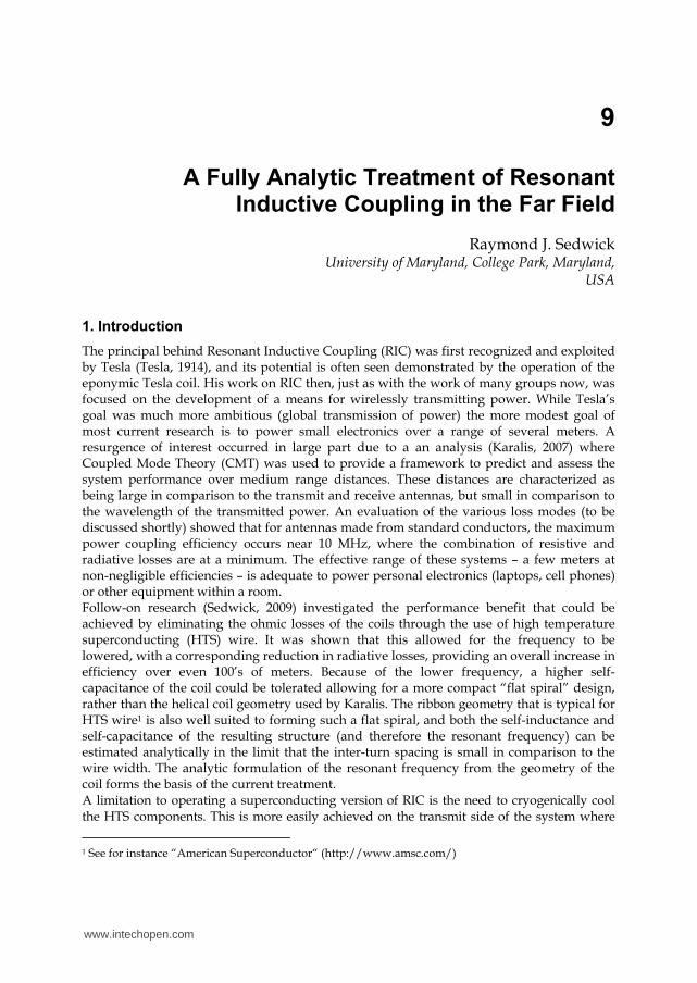
each coil. This phase dependence leads to the familiar exchange of energy between weakly

coupled systems as shown in Fig. 1 for a pair of un-driven resonant pendula.

In this figure, one pendulum (the Primary Oscillator) starts at a maximum energy and the

other starts at zero energy. In Eq. (6), this is equivalent to 1 2R Ia a= having a maximum value

and 1 2 0I Ra a= = . It is important to recognize that the amplitudes refer to the black envelope

lines in the figure, which oscillate at a frequency that is determined by the coupling constant

(κ ), rather than the blue curves, which oscillate at the resonant frequency of the system. The

actual positions of both pendula at 0t = are at their respective equilibrium locations (zero

offset angle), however the velocity of the first pendulum is a maximum, whereas the

velocity of the second pendulum is zero. After a quarter period, all of the energy has been

transferred to the second pendulum, except for that which has been lost by dissipation (Γ ).

Energy then flows back to the first pendulum over the next quarter period. Without loss of generality, we will always choose this phase relationship, and we will consider the steady-state situation where power is continuously supplied to the primary coil at the same rate that it is lost (both through dissipation and coupling to the secondary) and power is continuously coupled to the secondary coil at the same rate that it is lost (both

www.intechopen.com


176

Fig. 1. Exchange of energy between two weakly coupled pendula of the same frequency.

through dissipation and driving the load). In this state, both 1Ra and 2

Ia will remain

constant, although not necessarily having the same value. We will also recognize that for

this choice of phasing, 1 1 2 2, R Ia a a a= = .

The steady-state condition for the secondary coil is therefore given by

2 2

1 2 2 2 1 2 2( ) ( )W R O D Wa a a MI I R R R R Iκ ω= Γ + Γ ⇒ = + + + (7)

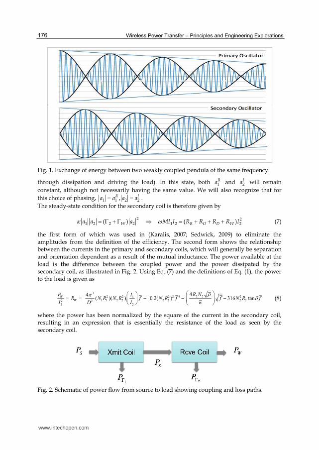
the first form of which was used in (Karalis, 2007; Sedwick, 2009) to eliminate the amplitudes from the definition of the efficiency. The second form shows the relationship between the currents in the primary and secondary coils, which will generally be separation and orientation dependent as a result of the mutual inductance. The power available at the load is the difference between the coupled power and the power dissipated by the secondary coil, as illustrated in Fig. 2. Using Eq. (7) and the definitions of Eq. (1), the power to the load is given as

PW

I2

2 = RW =

4π 3

D3(N1R1

2 )(N2R2

2 )I1

I2

⎛⎝⎜

⎞⎠⎟ f − 0.2(N2R2

2 )2 f 4 − 4R2N2 ρw

⎛⎝⎜

⎞⎠⎟ f − 316N2

2R2 tanδ f

(8)

where the power has been normalized by the square of the current in the secondary coil, resulting in an expression that is essentially the resistance of the load as seen by the secondary coil.

Fig. 2. Schematic of power flow from source to load showing coupling and loss paths.

www.intechopen.com


177

Previously, an expression of this form was used to find a frequency that optimized performance, assuming that the other parameters were fixed. However, for the close-packed spiral coil (of ribbon wire) being considered here, and assuming no other reactive components are present, the natural frequency of the coil is given by (Sedwick, 2009)

2 2 0.750.86

r r

d df NR f

R Nw wβε ε≈ ⇒ ≈ = (9)

where , d w appear from the calculation of coil capacitance. For other wire geometries the

parameters and numerical factors that appear on the right side may change, but the product 2 2NR f should persist, making it approximately constant from one coil to another for a

given wire packing and insulation. Inserting this into Eq. (8) we find

3 2

223 3 3

1 2 2

1316 tan4 4 0.2

( ) ( )W

II R

I R wfD f R f

β δπ β β ρβ−⎡ ⎤⎛ ⎞= = + + +⎢ ⎥⎜ ⎟⎢ ⎥⎝ ⎠⎣ ⎦ (10)

where the number of turns in the coil has been eliminated in lieu of the coil radius where appropriate. It is interesting to note that comparison of Eqs. (8) and (9) shows that the radiation resistance is completely specified by the details of the wire geometry and insulation. For a given primary coil current, the power delivered to the load at the secondary is then

2 2

22 1 02 2

W W W

I I IP R R I I

f

∂= = ⇒ =∂ (11)

since the currents are given as peak values rather than RMS. Also shown is the condition that would result in a frequency that maximizes the power delivered. However, in the current form there is no longer a peak in the power delivered. Instead, the power delivered increases toward lower frequencies, corresponding to an ever-increasing number of turns, since the radius has been assumed fixed in Eq. (10). At lower frequencies the effects of dielectric and ohmic losses are seen to become problematic, leading to the dielectricless, superconducting design considered in (Sedwick, 2009). The thermal overhead of a superconducting coil in some cases may be prohibitive, but a design that avoids the use of a dielectric is critical to achieving peak performance.

Differentiating the second expression for power given in Eq. (11) with respect to the load

resistance (assuming 1I is fixed), the maximum power is delivered when the load resistance

is equal to the total dissipation, a result also found in (Sedwick, 2009). This can be seen to

result from the fact that while a larger load will increase power for a given current, it will

also decrease the amount of current through Eq. (10). The maximum power occurs when the

load is as large as possible without overly limiting the current, i.e. when it is equal to the

dissipation.

2.1 Two superconducting, dielectricless coils

For the superconducting case (no ohmic or dielectric losses, and 20.2WR β= ), the parameter β is seen to cancel out of the current ratio, making the result independent of the wire

packing and producing the same equation identified as the figure of merit (FOM) given in

www.intechopen.com


178

(Karalis, 2007; Sedwick, 2009). Using Eq. (9), the maximum power delivered in the

superconducting case can be expressed solely in terms of coil design parameters as

6

2 3 21 2

6.1RW

w RP I N

Dd

⎛ ⎞⎛ ⎞≈ ⎜ ⎟⎜ ⎟⎝ ⎠⎝ ⎠ (12)

where it is seen that only the secondary coil parameters are present. The geometry of the primary coil is of course constrained implicitly by Eq. (9), but this coil need not be superconducting. For the power delivered in the non-superconducting case (but still with no dieletric), the resistive losses will dominate, and the load resistance should be matched to this quantity instead. In this case the expression for maximum power delivered is given as

1/4 6

2 2.25 21 2

2

3.4OW

w d RP I N

Dd Rρ⎛ ⎞ ⎛ ⎞= ⎜ ⎟ ⎜ ⎟⎝ ⎠ ⎝ ⎠ (13)

The ratio of maximum power delivered by a system with only radiative losses to one with mainly ohmic losses is then

3/4

2 233R

WOW

RP N w

d dP

ρ ⎛ ⎞≈ ⎜ ⎟⎝ ⎠ (14)

which will typically be on the order of a few thousand. For the same power delivered, this would mean a difference in range of a factor of about 3 to 4. To find the overall system efficiency we need to evaluate the amount of power required at the input of the primary coil. This can be found in a similar way to the power to the load in terms of the coupled power and the coil losses given by

1

3 222

2 2 3 3 31 11 1 1

316 tan4 4 0.2( ) ( )

SP PP I

I R wI I fD f R f

κ β δπ β β ρβΓ+ ⎛ ⎞ ⎛ ⎞= = + + +⎜ ⎟ ⎜ ⎟⎝ ⎠ ⎝ ⎠ (15)

where the substitutions using Eq. (9) have already been made. As before we will first assume the case when the coil is superconducting and with no dielectric, in which case the last two terms are zero. Assuming the maximum power transfer condition, the efficiency can be written

3 2

23

4 where , , 0.2/ 2( )

RW RR

RS

P P P x I xx I

P P x IP fDκκ

α π βη α βα α− −= = = = = =+ + (16)

Elimination of frequency using Eq. (9) results in

3 62

1,2 1,2

1 1

2 4 29.85

d D

x wN R

αη−− ⎡ ⎤⎡ ⎤ ⎛ ⎞ ⎛ ⎞⎛ ⎞ ⎢ ⎥= + ≈ +⎢ ⎥ ⎜ ⎟ ⎜ ⎟⎜ ⎟ ⎜ ⎟ ⎜ ⎟⎢ ⎥⎝ ⎠⎢ ⎥ ⎝ ⎠ ⎝ ⎠⎣ ⎦ ⎣ ⎦

(17)

where the number of turns and radius of either coil can be used as long as they are

consistent. The radius and number of turns for either the primary or secondary coil can be

www.intechopen.com


179

used since they must be related by the frequency matching condition. The maximum

efficiency is seen to be 50% because for the maximum power transfer the load power is

equal to the dissipated power in the secondary coil, and in the limit of 0α → the dissipated

power in the primary coil becomes negligible to that in the secondary. For a nominal coil

design, with the values / 4, 100w d N= = , the efficiency drops to 10% when the coils are

separated by about 280 radii.

2.2 Two non-superconducting, dielectricless coils

For the non-superconducting case, the ohmic losses will dominate the coil. We will assume at first that both the primary and the secondary are non-superconducting. The only change from Eq. (17) is the definition of α , which is now the ohmic resistance, and is unique to

each coil based on its radius. This gives

η = 2 + 4α1α2

x2

⎡⎣⎢

⎤⎦⎥−1

α1,2 = 4βR1,2w

⎛⎝⎜

⎞⎠⎟

ρf 3

(18)

Again eliminating the frequency we find

622

1.51 22

1

23.07

d R D

w R RwdN

ρη−⎡ ⎤⎛ ⎞⎢ ⎥= + ⎜ ⎟⎢ ⎥⎝ ⎠⎣ ⎦

(19)

which is shown expressed in terms the secondary coil, although the radius of the primary coil does appear. Swapping all of the indices will result in the same efficiency as a result of the frequency matching condition. For two of the nominal coils as described above, with the additional information of having identical radii of 0.5 m, wire width of 4 mm and formed from copper wire, the efficiency drops to 10% when the coils are separated by 20 radii. This is a distance of just over 9 meters, as compared to 140 meters for the superconducting case.

2.3 A hybrid set of dielectricless coils

The form of the efficiency given in Eq. (18) lends itself nicely to considering hybrid system

designs, since the expressions for 1,2α can refer to coils with different losses. However,

remarkably the efficiency is completely symmetric with respect to which coil is the primary

versus the secondary. The reason that this is unexpected is that one of the coils could have

substantially more current, and one might expect that making this coil superconducting

would result in a more efficient design. Let us assume that a system has a superconducting

primary and a non-superconducting secondary, and that the ratio of losses is a factor of

1λ > . Swapping coils will decrease the resistance of the secondary by λ (assuming the load

remains matched to the secondary losses), resulting in an increase in I by this same factor.

Assuming the same power to the load, the current in the secondary must increase by a factor

of λ , which means that the current in the primary must be reduced by this same factor to

keep the coupled power constant. The resistance of the primary is now larger by a factor of λ (the resistive coil), so the power dissipated in the primary remains the same. If the load

power and dissipated powers all remain the same, so does the efficiency. The advantage of this is that a superconducting coil can be introduced on either side of the system and will have the same effect of increasing the system efficiency. Since the

www.intechopen.com


180

superconducting coil will have some thermal management overhead that will require power (a power which has not been accounted) it would be more useful to put it at the end of the system that is transmitting the power, where power is plentiful. However, in the case of using the system for communications (which is discussed next), both sources would have their own power supply and signals could be transmitted bi-directionally. If one of the systems has an ample supply of power, whereas the other has a limited supply of power, the superconducting coil can be placed at the power rich side for the benefit of both ends. As a final consideration in this section, the efficiency of a hybrid system is given as

1.25 6

21 22 2.25

22

1 1

2 4 25.50

Rd D

w Rx wN

ρα αη−− ⎡ ⎤⎛ ⎞ ⎛ ⎞⎡ ⎤ ⎢ ⎥= + ≈ + ⎜ ⎟ ⎜ ⎟⎢ ⎥ ⎢ ⎥⎣ ⎦ ⎝ ⎠⎝ ⎠⎣ ⎦

(20)

For a hybrid system with the parameters specified above, the efficiency drops to 10% at a distance of 75 radii, which is the geometric mean of the distances for the other two cases as might be expected. Again the efficiency is expressed in terms of the secondary coil parameters, but can be expressed in terms of the primary by changing all of the indices.

3. Application to communications

While the efficiency drops off rapidly, one application that does not require an efficient transfer of power is communications. For example, if a receiver requires a microwatt of power to get a signal, but the transmitter is operating at only one Watt of power, the efficiency is 10-6, but the system works as desired. Thus far, coupled mode analysis has been used to assess the power transfer and efficiency between resonant coils of similar designs with potentially different loss characteristics. However, the only frequency present was the resonant frequency of the system. To assess the applicability of such hybrid systems for communications, an approach must be used to capture the effect of broad-spectrum coupling. For the purpose of transmitting signals, only three coil components will be assumed: A drive coil which is non-resonant, and a pair of resonant coils, which as previously may each have different loss characteristics. Demodulation of the signal on the secondary side will be assumed to occur directly off the secondary coil since it will provide the largest voltage. The drive coil is driven at the resonant frequency of the tuned coils, but only couples strongly to the primary coil due to both its proximity and limited magnetic flux generation. The signal into the drive coil is encoded using amplitude modulated. To proceed with the analysis, a sign convention will be established whereby current traveling clockwise around a coil (as viewed from the primary to the secondary coil, assuming that they are axially aligned) is considered positive, while a counter-clockwise current is negative. The model for all three coils is the same (see Fig. 3), with capacitive and inductive elements having series resistors to capture the various loss modes. Beginning with the secondary coil, the governing equation is given as

1S S S S S PS P

S

L I R I q emf M IC

+ + = = −$ $ (21)

where , S SI q are the current and unbalanced charge in the coil, , S SL R and SC are the

effective inductance, resistance and capacitance of the coil and emf is the electromotive

www.intechopen.com


181

Fig. 3. Electrical model of drive, primary and secondary coils.

force induced in the secondary coil by the changing current in the primary. The resistance

includes both SCR (dielectric loss) and S

LR (ohmic and radiative coil losses). An increasing

positive current in the primary will induce a negative emf in the secondary by Lentz’s Law,

proportional to the mutual inductance ( PSM ) between the two coils. Differentiating with

respect to time yields

202 PS

S S S S PS

MI I I I

Lω+ Γ + = −$$ $ $$ (22)

where SΓ is the decay rate as defined previously using CMT. Similarly, the governing

equation for the primary is

202 PD

P P P P DP

MI I I I

Lω+ Γ + = −$$ $ $$ (23)

where the back emf from the secondary has been neglected because it will be very small

compared to the drive coil emf .

3.1 Drive coil

Treatment of the drive coil is different, since it is not driven inductively, but instead directly by an amplifier stage. It consists nominally of a single loop of wire in close proximity to the primary and has a resonant frequency that would typically be much higher than the operating frequency of the system. Current driven around the coil from the amplifier is effectively traveling through the inductive and capacitive legs in parallel, so its impedance can be found as

2( ) ( )1 1 / ( ) ( )

D

D

D

D

D D D DL C D D C L

D D D D DL D C D L C D

R R X jX R RZ

R j L R j C R R jX

ωωω ωωωω ωω ω

+ + −⎛ ⎞= + =⎜ ⎟⎜ ⎟+ − + + −⎝ ⎠ (24)

where the resistance values are as shown in Fig. 3, and DX is the reactance of both the

inductor and capacitor at the drive coil’s resonant frequency ( Dω ). Since this frequency is so

much higher than the operating frequency of the primary and secondary coils, the

impedance of the drive coil reduces to

DD L DZ R j Lω= + (25)

www.intechopen.com


182

at all relevant frequencies. For a given applied voltage, ( )DV ω , the current in the coil is

simply found from Ohm’s law. Assume an amplitude modulated voltage of the form

0 0 00

( ) ( ) sin (1 cos ) Im[ ] , ( )2

D m m D Dj t j t j tV V t t V V V e e eω ω ω ω ωγω γ ω + −= + = = + + (26)

where mV is the amplitude of the carrier, γ is the amplitude of the modulation relative to

the carrier, 0ω is the carrier frequency (resonant frequency of the primary and secondary

coils) and ω is the frequency of the modulation. The complex form will be used throughout

the analysis for simplicity, allowing the appropriately phased solution to be found at any

point by taking the imaginary component.

It should be noted that a substantial back emf from the primary will be seen across the

drive coil, so that the voltage driving the current in the drive coil will actually be

S m D PD PV V V M I= − $ (27)

Knowing this, we will assume for simplicity that this back emf has been compensated by

the amplifier, so that Eq. (26) represents SV , the net voltage seen across the drive coil.

3.2 Primary coil

The current in the primary coil is found by solving Eq. (23), driven by SV (~ DV )

202

( )PD m

P P P P DP D D

M VI I I V

L R j Lω ω+ Γ + = − +

$$$$ $ (28)

where

0 0 02 2 2 20 0 0 0

( ) ( ) [ ( ) ( ) ] 2

D Dj t j t j tV e e e Vω ω ω ω ωγω ω ω ω ω ω+ −= − + − + − − ≈ −$$ (29)

In the last form of Eq. (29) (far right), the impact of ω versus 0ω on the amplitude of the

signal has been neglected. This is a good approximation since the modulation frequency will

be small in comparison to the resonant frequency and this approximation will be made

throughout the analysis. Similarly, for the current of the drive coil we will assume

0 0 0 0

0 0 0 0

( ) ( )

and ( )D D D D D D

j t j t j t j te e e e

R j L j L R j L j L

ω ω ω ω ω ωω ω ω ω ω

± ±≈ ≈+ + ± (30)

where we have neglected the small relative phase shift introduced by the modulation and

by the resistance of the drive coil. While the transient homogeneous solution to Eq. (28) will

play a role under a continuously varying input signal, for the present analysis we are merely

concerned with the frequency response of the driven system. Assuming a particular solution

of the form Pj t

I eω , Eq. (28) becomes

2 2 00( 2 ) PD m

P P SP D

M Vj I j V

L L

ωω ω ω ⎛ ⎞+ Γ − = − ⎜ ⎟⎝ ⎠ (31)

www.intechopen.com


183

Solving Eq. (31), each of the terms from SV couple into the current of the primary as

0 00 0 ))

2 2 2 2 2 200 0 0 0 0 0 0 0

(( ( ) , 22 ( ) 2 ( ) 2 ( )

P

PP P P

j t j tj t j tje j j ee e

j j

ωωω ωω ω ωωω ω ω ω ω ω ω ω ω ω

±±− − Γ⇒ ⇒Γ− + Γ − ± + Γ ± Γ +∓

(32)

and the complete expression for the current in the primary coil becomes

( )0 0 0

2) )*

2 2 2 20 0

( ( , 2 2

PD m P PP P P P

P D P P P

j t j t j tM VI e c e c e c j

L L

ω ωω ω ωγ ωω ω

+ − Γ Γ⎡ ⎤= − + + = +⎢ ⎥Γ Γ + Γ +⎣ ⎦ (33)

Because of the close proximity of the drive coil to the primary, if we assume that the radii of both coils are the same, then nearly all of the flux generated by one coil will thread the other. This is equivalent to saying that the coupling coefficient (κ ) is nearly unity. However in general, the mutual coupling between the drive and primary coils can be given in terms of

the inductance of either coil as P D

D P

N NPD D P D PN N

M L L L Lκ κ κ= = = . Using the first expression

with 1DN = , and substituting in for the physical definition of PΓ , the primary current is

( )0 0 0) )* ( (

2( )P m

P P PP PL C

j t j t j tN VI e c e c e

R R

ω ωω ω ωκ γ + −⎡ ⎤= − + +⎢ ⎥+ ⎣ ⎦ (34)

Although it may not be surprising to see the familiar Ohm’s law relationship with a transformer step-up, there are two subtleties worth noting. The first is that the reactive component of the coil impedance does not appear, which is at first striking because the high Q of these coils implies that the reactive part should dominate. The second point to note is that the primary coil is not simply being driven as the “secondary” of a standard transformer, but rather at the resonance frequency of the primary. Therefore the peak voltage across the primary should well exceed the step-up resulting from simply taking the turns ratio of the transformer. These two points actually resolve themselves if we recognize that it is the reactance of the coil that actually drives it to high voltages at resonance. So,

given the current found in Eq. (34), the peak voltage across the primary is not in fact P mN V ,

but rather 0 0peak P P pV I X I L ω= = . The real power dissipated in the coil is however just

P P mI N V or

2

2( ) ( )P P PP mLoss P L CP P

L C

N VP I R R

R R= = ++ (35)

While it is true that for a given drive voltage, decreasing the primary coil resistance actually

increases the power dissipation, the goal is to achieve a certain level of current. Given PI ,

reducing the coil resistance reduces both the power loss as well as the voltage that must be

generated by the amplifier.

We can now consider the back emf in the drive coil that must be compensated. This is given

by

0 0 ( ) ( )

emf P m PDPD p P m m PD P P P P

P L C L C

N V j LNV M I L j V j V Q

N R R R R

ω ωκ κ κ⎛ ⎞= − = − = − = −⎜ ⎟ + +⎝ ⎠$ (36)

www.intechopen.com


184

so that whatever the desired mV , the back emf to be compensated will lag by 90˚ and be

greater in amplitude by a factor of PQκ , the product of the coupling constant and the

quality of the primary coil. Looking now at the complex part of the primary current, taking the imaginary component results in

2

0 2 2 2 2sin 1 cos sin

( )P m P P

P P PL C P P

N VI t t t

R R

κ ωω γ ω ωω ω⎡ ⎤⎛ ⎞Γ Γ= − + +⎢ ⎥⎜ ⎟⎜ ⎟+ Γ + Γ +⎢ ⎥⎝ ⎠⎣ ⎦

(37)

and in the desired low-loss limit, this becomes approximately

0sin 1 sin( )

P m PP P P

L C

N VI t t

R R

κ ω γ ωωΓ⎡ ⎤= − +⎢ ⎥+ ⎣ ⎦ (38)

where low-loss assumes that the dissipation factor is small in comparison to the modulation frequency. If we consider at what frequency the modulated signal is reduced to 50% of its original value, we find

0 0 0

2 1 2 2

P PP

P P P

R R

L L Q

ωω ω ω ω= Γ ⇒ = = = (39)

So, as expected, the bandwidth that can be supported by the system is governed by the resonant frequency and the quality of the oscillator. To achieve both high efficiency and bandwidth, the frequency of operation should then be as high as possible. Since high frequency corresponds to radiative losses in an inductively coupled system of a given size, this sets fundamental constraints on efficiency and bandwidth. However, it also indicates that reducing the ohmic and dielectric losses in favor of radiative losses is a way to maximize bandwidth and efficiency. If it is desired to maintain low detectability, the radiated energy must be shielded in some way such as by using a Faraday cage.

3.3 Secondary coil

Continuing now to the secondary coil, the governing equation for the current is given by Eq.

(22), with the driving current given by Eq. (34). As before, 20S SI Iω≈ −$$ resulting in

( )0 0 0

2) )2 2 2 *0

0 0( (( 2 )

2( )PS PS P m

S S P P PP PS S L C

j t j t j tM M N Vj I I e c e c e

L L R R

ω ωω ω ωω γω ω ω ω + −⎡ ⎤+ Γ − = = + +⎢ ⎥+ ⎣ ⎦ (40)

After similar machinations as before, the current in the secondary can be given as

( )0

2 2* * *0

2 2 2 20 0

1 , 2( )

PS P m S SS S P P P SP P

S L C S S

j t j t j tM N VI je c c e c c e c j

L R R

ω ω ωω ωγω ω

− Γ Γ⎡ ⎤= + + = +⎢ ⎥+ Γ + Γ +⎣ ⎦ (41)

Expressing the mutual inductance and self-inductances in terms of system parameters as in Section 2, the amplitude of the current in the secondary becomes

32 22 2

03

4 2( ) ( ) ( )

mPS P m S SP PS P P P P S S

L C S S L C L C

V fM N V N RN RI

R R L R R R R D

πω ⎛ ⎞⎛ ⎞= = ⎜ ⎟⎜ ⎟⎜ ⎟⎜ ⎟+ Γ + +⎝ ⎠⎝ ⎠ (42)

www.intechopen.com


185

Dividing out the current in the primary we find

3 32 2 2 2

23 3

1

4 4 ( )

P P S S P P S SS S

W RadL C

f fN R N R N R N RI

I R RR R D D

π π⎛ ⎞ ⎛ ⎞= = =⎜ ⎟ ⎜ ⎟⎜ ⎟ ⎜ ⎟++⎝ ⎠ ⎝ ⎠

2 4 3 3 2

22 3 3

1/ 4 4 0.20.2 ( )

WW

f fR

R D fD

β π π β ββ−⎛ ⎞ ⎡ ⎤= = +⎜ ⎟ ⎣ ⎦⎜ ⎟+⎝ ⎠ (43)

where we have eliminated all losses except for radiative, added in an equivalent series resistance for the load and substituted in definitions from Eqs. (3) and (9). Gratifyingly, the final expression on the right is identical to that of Eq. (10), under the same set of assumptions. Taking only the imaginary component of Eq. (41), the current corresponding to our assumed input in the low-loss operating limit is

322 2

03 2

4cos 1 cos

( ) ( )mS S P SP P

S P P S SL C L C

V fN RN RI t t

R R R R D

π ω γ ωω⎛ ⎞⎛ ⎞ Γ Γ⎡ ⎤= −⎜ ⎟⎜ ⎟ ⎢ ⎥⎜ ⎟⎜ ⎟+ + ⎣ ⎦⎝ ⎠⎝ ⎠ (44)

Considering the coefficient of the modulated waveform as before, the bandwidth based on a 50% reduction in amplitude is given by

2

002

1 1 4 2 2

P S

P S P S

ff

Q Q Q Q

ωωω

Γ Γ ⎛ ⎞= = ⇒ Δ =⎜ ⎟⎝ ⎠ (45)

and can be seen to be related to the geometric mean of the primary and secondary coil Q-factors. As an example, we will assume an operating frequency of 10 MHz, a frequency where the radiative losses begin to be comparable to ohmic losses. Voice transmission has a bandwidth typically taken to be 4kHz2, so the combined system Q-factor can be as high as 1800 using Eq. (45). If radiative losses are the only dissipation in the system, then the Q-factor of each coil can be calculated as

2 2 2

02 2 2 3 3

32 160 11.6 0.2( ) ( )Rad

N RfLQ Rf

R NR f Rf Q

πω π= = = ⇒ = (46)

At 10 MHz, 1f = , so 0.95R m= from Eq. (46), but the number of turns in the coils is

unspecified since both radiative resistance and reactance scale as 2N . At 1MHz, the Q-factor

would need to be 10 times smaller to support the required bandwidth, requiring the coil

radius to be over 21 times larger. However, there is no need to require that the dissipation

be purely radiative, and only a small amount of additional dissipation is needed to

substantially reduce the Q-factor.

4. Range of detection and bandwidth

For a given demodulation threshold, the ability to detect and demodulate the signal from the carrier is distance dependent by the overall strength of the received signal. The

2 See for instance http://en.wikipedia.org/wiki/Voice_frequency

www.intechopen.com


186

maximum voltage that will be seen across the secondary coil can be found from the current induced and the Q-factor of the coil, as was discussed with the primary coil. The modulated signal will then be attenuated as shown in Eq. (45). For the case of a superconducting secondary, these can be combined to yield

73

max 03 3 * 2

22 3101 5 2490

4 ( )S P P

S S S P SP P S P P

fI I IV I Q I Q

I Q Q Q f Df D Q f f

ω πω

⎛ ⎞⎛ ⎞⎛ ⎞⎛ ⎞ ⎛ ⎞ ⎛ ⎞= = = ≈⎜ ⎟⎜ ⎟⎜ ⎟⎜ ⎟ ⎜ ⎟⎜ ⎟ ⎜ ⎟⎜ ⎟Δ Δ ⎝ ⎠⎝ ⎠⎝ ⎠⎝ ⎠ ⎝ ⎠⎝ ⎠ (47)

where PQ and PI have been left explicitly and the bandwidth ( *fΔ ) is in kHz. The reason

is that all of the factors in the final form would be operationally derived. For instance, while an arbitrarily high primary current may be theoretically possible, power limitations or wire current capacity would most likely limit it to a maximum value. Likewise, there is no constraint on making the Q-factor of the primary large or small, so we allow it to be specified directly. The Q-factor of the secondary is seen to cancel, since while it reduces the current in the secondary it also increases the peak voltage. Although this cancellation occurs (making its value irrelevant), the relationship used for the current ratio has already assumed that only radiative losses are seen in the secondary and that the load power is negligible by

comparison. In general, however, Eq. (10) can be used to find /S PI I for any dominant loss

mode.

The achievable bandwidth and carrier frequency are not independent of the values of PQ

and SQ , and Eq. (45) can be used to conservatively replace the carrier frequency in lieu of

the Q-factors. This results in

4

max ** 3 max

313(10 ) 2490 47800

2 ( )P P

SP P S S P P S

I IV f

D DQ Q Q f V Q Q Q

⎛ ⎞⎛ ⎞ ⎛ ⎞≈ ⇒ Δ ≈ ⎜ ⎟⎜ ⎟ ⎜ ⎟⎜ ⎟Δ ⎝ ⎠ ⎝ ⎠⎝ ⎠ (48)

Under the present assumptions, a selection of threshold voltage, primary coil current, Q-

values, and operating distance will determine the bandwidth. As an example, assume that

the detection threshold is 20 mV, about four times the typical laboratory noise floor. Parallel

windings of wire could allow for a recirculating primary current of 100 Amps, and quality

voice communications would require 4f kHzΔ = ( )* 4fΔ = . High Q-factors are seen to be

detrimental, however since the secondary has been assumed superconducting, the

expectation is that SQ will nevertheless be quite large – on the order of 106. The variation of

bandwidth with distance for three values of PQ is shown in Fig. 4. A consequence of using a high-Q coil as a secondary is that the Q-factor of the primary must be smaller to support a given bandwidth. This translates into higher power requirements on the primary. For the case of a receiver coil that is dominated by ohmic losses, the modulated signal strength across the secondary coil is given instead by

73

max 0 2 2* 23 3

22 3101 1460

4 ( )S P P

S P SP P S P P

f fI I R w I R wV I Q

I Q Q Q f DQ fD f

ω π β βω ρρ

⎛ ⎞⎛ ⎞⎛ ⎞ ⎛ ⎞ ⎛ ⎞= = ≈⎜ ⎟⎜ ⎟⎜ ⎟ ⎜ ⎟⎜ ⎟ ⎜ ⎟Δ Δ ⎝ ⎠⎝ ⎠⎝ ⎠⎝ ⎠ ⎝ ⎠ (49)

where the ohmic term in Eq. (10) has been used for the current ratio between the secondary

and the primary. Using the same substitution to eliminate the carrier frequency results in

www.intechopen.com


187

23 21/4 1/4 3

max ** 3/2 max

( ) ( )353 321 ( )

P S P S P S P SS

P P S

Q Q I R w Q Q I R dV f

D DQ f Q V

βρ ρ

⎛ ⎞⎛ ⎞ ⎛ ⎞≈ ⇒ Δ ≈ ⎜ ⎟⎜ ⎟ ⎜ ⎟⎜ ⎟Δ ⎝ ⎠ ⎝ ⎠⎝ ⎠ (50)

The frequency dependency now weakly favors a higher SQ , which is now unfortunately

much smaller as a result of the ohmic losses in the secondary. Using the additional

assumptions of 0.5 , 1 , 1.6SR m d mm ρ= = = along with the same previously assumed

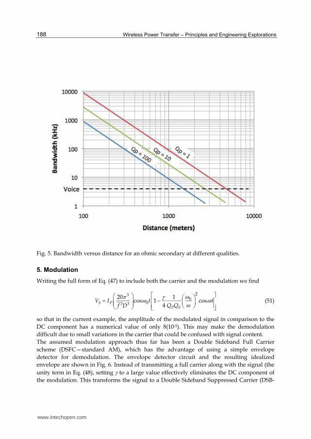
parameters, the bandwidth is plotted as a function of distance in Fig. 5 for the same values

of PQ assumed in Fig 4.

Fig. 4. Bandwidth versus distance for a superconducting secondary at different qualities.

The range is seen to be smaller overall for the ohmic loss case, and in both cases the distance

is seen to increase as the Q-factor of the primary is decreased. The implication of reducing

the primary Q-factor is a greater amount of power that must be expended. It should be

noted that by fixing the Q-factors of the primary and secondary coils for the performance

curves shown in Figs. 4 and 5, the assumed carrier frequency is changing for different values

of bandwidth. These plots, therefore, do not show the reduction in bandwidth with distance

of a fixed system design, but rather how the baseline design would change for different

maximum ranges of operation. To see how the bandwidth of a particular system would roll

off with distance would require going back to Eqs. (47) and (49).

www.intechopen.com


188

Fig. 5. Bandwidth versus distance for an ohmic secondary at different qualities.

5. Modulation

Writing the full form of Eq. (47) to include both the carrier and the modulation we find

3

003 3

220 1

cos 1 cos4

S PP S

V I t tQ Qf D

ωπ γω ωω⎡ ⎤⎛ ⎞ ⎛ ⎞= −⎢ ⎥⎜ ⎟ ⎜ ⎟⎜ ⎟ ⎝ ⎠⎢ ⎥⎝ ⎠ ⎣ ⎦

(51)

so that in the current example, the amplitude of the modulated signal in comparison to the

DC component has a numerical value of only 8(10-5). This may make the demodulation

difficult due to small variations in the carrier that could be confused with signal content.

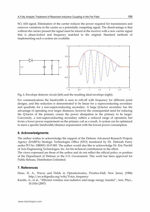
The assumed modulation approach thus far has been a Double Sideband Full Carrier

scheme (DSFC—standard AM), which has the advantage of using a simple envelope

detector for demodulation. The envelope detector circuit and the resulting idealized

envelope are shown in Fig. 6. Instead of transmitting a full carrier along with the signal (the

unity term in Eq. (48), setting γ to a large value effectively eliminates the DC component of

the modulation. This transforms the signal to a Double Sideband Suppressed Carrier (DSB-

www.intechopen.com


189

SC) AM signal. Elimination of the carrier reduces the power required for transmission and

removes variations in the carrier as a potentially competing signal. The disadvantage is that

without the carrier present the signal must be mixed at the receiver with a new carrier signal

that is phase-locked and frequency matched to the original. Standard methods of

implementing such a system are available.

Fig. 6. Envelope detector circuit (left) and the resulting ideal envelope (right).

For communications the bandwidth is seen to roll-off with frequency for different point

designs, and this reduction is demonstrated to be linear for a superconducting secondary

and quadratic for a non-superconducting secondary. A large Q-factor secondary has the

advantage of operating over larger distances, however the consequential need for reducing

the Q-factor of the primary causes the power dissipation in the primary to be larger.

Conversely, a non-superconducting secondary suffers a reduced range of operation, but

levies a lower power requirement on the primary coil as a result. A system can be optimized

to meet a specific bandwidth/distance requirement with the lowest power consumption.

6. Acknowledgments

The author wishes to acknowledge the support of the Defense Advanced Research Projects

Agency (DARPA) Strategic Technologies Office (STO) monitored by Dr. Deborah Furey

under PO No. HR0011-10-P-003. The author would also like to acknowledge Dr. Eric Prechtl

of Axis Engineering Technologies, Inc. for his technical contributions to the effort.

The views expressed are those of the author and do not reflect the official policy or position

of the Department of Defense or the U.S. Government. This work has been approved for

Public Release, Distribution Unlimited.

7. References

Haus, H. A., Waves and Fields in Optoelectronics, Prentice-Hall, New Jersey (1984) http://en.wikipedia.org/wiki/Voice_frequency

Karalis, A., et al., “Efficient wireless non-radiative mid-range energy transfer”, Ann. Phys., 10.1016 (2007)

www.intechopen.com


190

Sedwick, R.J.,“Long range inductive power transfer with superconducting oscillators“, Ann. Phys., 325 (2010) 287–299.

Tesla, N., U.S. patent 1,119,732 (1914)

www.intechopen.com

Wireless Power Transfer - Principles and Engineering ExplorationsEdited by Dr. Ki Young Kim

ISBN 978-953-307-874-8Hard cover, 272 pagesPublisher InTechPublished online 25, January, 2012Published in print edition January, 2012

InTech EuropeUniversity Campus STeP Ri Slavka Krautzeka 83/A 51000 Rijeka, Croatia Phone: +385 (51) 770 447 Fax: +385 (51) 686 166www.intechopen.com

InTech ChinaUnit 405, Office Block, Hotel Equatorial Shanghai No.65, Yan An Road (West), Shanghai, 200040, China

Phone: +86-21-62489820 Fax: +86-21-62489821

The title of this book, Wireless Power Transfer: Principles and Engineering Explorations, encompasses theoryand engineering technology, which are of interest for diverse classes of wireless power transfer. This book is acollection of contemporary research and developments in the area of wireless power transfer technology. Itconsists of 13 chapters that focus on interesting topics of wireless power links, and several system issues inwhich analytical methodologies, numerical simulation techniques, measurement techniques and methods, andapplicable examples are investigated.

How to referenceIn order to correctly reference this scholarly work, feel free to copy and paste the following:

Raymond J. Sedwick (2012). A Fully Analytic Treatment of Resonant Inductive Coupling in the Far Field,Wireless Power Transfer - Principles and Engineering Explorations, Dr. Ki Young Kim (Ed.), ISBN: 978-953-307-874-8, InTech, Available from: http://www.intechopen.com/books/wireless-power-transfer-principles-and-engineering-explorations/a-fully-analytic-treatment-of-resonant-inductive-coupling-in-the-far-field

© 2012 The Author(s). Licensee IntechOpen. This is an open access articledistributed under the terms of the Creative Commons Attribution 3.0License, which permits unrestricted use, distribution, and reproduction inany medium, provided the original work is properly cited.

http://creativecommons.org/licenses/by/3.0

A Fully Analytic Treatment of Resonant Inductive Coupling in the

Documents