A full-chain, temporary network model with sliplinks, chain-length fluctuations, chain connectivity and chain stretching

A Full-Chain, Temporary Network Model with

Sliplinks, Chain-length Fluctuations, Chain

Connectivity and Chain Stretching∗

Jay D. Schieber, Jesper Neergaard and Sachin GuptaCenter of Excellence in Polymer Science and Engineering and

Chemical and Environmental Engineering Department

Illinois Institute of Technology, Chicago, IL 60616-3793

October 17, 2002

Abstract

A full-chain, temporary network model is proposed for nonlinearflows of linear, entangled polymeric liquids. The model is inspiredby the success of a recent reptation model, but contains no beads ortubes. Instead, each chain uses a different (and smaller) set of dy-namic variables: the location of each entanglement, and the numberof Kuhn steps in chain strands between entanglements. As before, themodel requires only a single phenomenological parameter that is fit bylinear viscoelasticity. The number of Kuhn steps varies stochasticallyfrom imbalances in chemical potential, and Brownian forces. In thelanguage of reptation, the model exhibits chain connectivity, chain-length fluctuations, chain stretching, and tube dilation. The currentimplementation in this framework does not include constraint release,although its addition is possible. The entanglements are assumed tomove affinely. Because of the affinity assumption and lack of con-straint release, the model should be expected to approximate well alinear chain in a matrix of fixed obstacles, and somewhat less accu-rately a polymer melt. Straightforward modifications to these assump-tions allow us to consider chains of any architecture in concentrated

∗Dedicated to Professor G. Marrucci on the occasion of his 65th birthday.

1

Journal of Rheology, in press 2

solutions or melts. A simulation algorithm for the model is describedin detail. Stress results are encouraging, since the model performs atleast as well as a complete tube model without constraint release atmuch lower computational cost. Finally, we consider possible gener-alizations of the proposed model, to include additional physics, suchas constraint release, branching, and non-affine motion.

I Introduction

Reptation ideas [de Gennes, 1971; Doi and Edwards, 1978a,b,c] have pro-vided a very useful conceptual framework for predicting the dynamics andstresses of entangled polymers. Quantitative predictions are now becomingpossible for a number of flows. However, some important limitations remain.Aside from the inability to describe all experiments, oftentimes wholly newmathematical models are created to attack the problem at hand. Hence,there exists no single mathematical model from which one may begin to at-tack any available problem. In fact, the list of variables necessary to describethe system is not universally accepted. So, while many of the importantadditional physical ideas, such as constraint release [des Cloizeaux, 1988;Tsenoglou, 1987], convective constraint release [Marrucci, 1996], or contour-length fluctuations [Doi and Edwards, 1986; Ketzmerick and Ottinger, 1989]have been identified, a suitable framework to incorporate these ideas stillappears to be lacking.

A previously proposed reptation model including information about anentire mean-field chain [Hua and Schieber, 1998a] has been shown to makegood quantitative comparison with stresses in double-step strains [Hua et al.,1998], inception and relaxation of steady shearing flows, steady shearing flows[Hua et al., 1999], and exponential shear flows [Neergaard et al., 2000]. Infact, the model made successful predictions , instead of mere descriptions ofthe data, and was essential in guiding our understanding of exponential shearflows and their connection to steady shearing flows.

This previous model incorporates chain connectivity, chain-length fluctu-ations, chain stretching and constraint release; this last effect is incorporatedin a self-consistent, mean-field way assuming binary chain entanglements,but the other effects follow in a self-consistent manner from the mechani-cal model proposed. The model uses one phenomenological parameter: amonomeric friction coefficient that is fixed from equilibrium data. All non-

Journal of Rheology, in press 3

linear viscoelastic predictions are then made without adjustable parameters.Despite the good agreement with experiments on an entangled polystyrene

solution, some drawbacks remain. First, the model is somewhat expensivecomputationally, prohibiting its use in most complex geometry calculations.Secondly, there are still some discrepancies with data: the steady-state ex-tinction angle approaches zero with increasing shear rate instead of reachinga plateau, and the magnitude of the overshoots in viscosity and normal stressduring inception of steady shear is overpredicted.

The physical implications of these discrepancies with experiment are notyet clear. The discrepancy in overshoot magnitude may be related to exces-sive stretching of the chain during the transient flow. This extra stretchingmay be related to the existence in the model of artificial Brownian particles,or beads, in the chain. Surprisingly, models containing very similar physics,but on a lower level of description do not show this problem [Fang et al., 2000;Mead et al., 1998; Ottinger, 1999]. In fact, [Mead et al., 1998] underpredictthe overshoot.

In this work, we propose a new mean-field model (first considered in[Schieber, 2000]) which incorporates the useful features of the earlier tubemodel, but offers a more natural implementation of the physical ideas. Theformulation of temporary network models provides a very useful mathemat-ical and conceptual framework towards this end (For an overview, see [Birdet al., 1987;Chapter 20], or, for example, [Petruccione and Biller, 1988; Vra-hopoulou and McHugh, 1987]). However, the new implementation has twoimportant differences from traditional network models. First, instead of pos-tulating phenomenological creation and destruction probabilities, the ideasfrom reptation are used. Secondly, the number of monomers in an entan-gled strand is not a constant parameter in the model, but rather a dynamic,fluctuating quantity.

In the following section we describe the dynamical model and propose itsevolution equation. In §III explicit expressions for the chain free energies areconsidered. We describe a simulation algorithm in §IV. Flow predictions aremade in §V for inception and steady shear flows. Finally, in §VI we discussoptions for future work and possible generalizations of the proposed theory.

Journal of Rheology, in press 4

II Model Description

The model uses the following dynamical variables for a single mean-fieldchain.

• There are Z(t)−1 entanglements in the chain. Hence, there exist Z−2entangled strands, and a total of Z strands in the chain. This valuecan fluctuate, but has an equilibrium value Zeq ≡ 〈Z〉eq given by themolecular weight M divided by the entanglement molecular weight Me.Sometimes it is more convenient to use the labels for the front and backstrands, if(t) and ib(t), which are allowed to fluctuate among integervalues such that if ≥ ib and Z = if − ib + 1.

• Strand i has Ni(t) Kuhn steps.

• Each entanglement point on the chain has position Ri(t) , i = ib, . . . , if−1. However, it is typically more convenient to keep track of the vectorsconnecting these entanglements along the chain Qi(t) := Ri − Ri−1,i = ib + 1, . . . , if − 1.

The physical picture described by the model is sketched in Figure 1 for achain of seven entanglements.

II.A Statics

We wish the chain to have an equilibrium distribution given by

peq(Ω) = J−1 exp

[

−F (Ω)

kBT

]

δ

(

NK −Z∑

i=1

Ni

)

, (1)

where the chain configuration is given by the shorthand notation Ω := Qi, Niifib

≡ Qib+1, . . . ,Qif−1, Nib , . . . , Nif , J is a normalization constant, kB is Boltz-mann’s constant, T is temperature, and F is the chain free energy

F =

if−1∑

i=ib+1

FS(Qi, Ni) + FE(Nib) + FE(Nif ), (2)

where the free energies of an entangled strand FS and end strand FE must bespecified. Examples for these are given in §III, but for the time being we may

Journal of Rheology, in press 5

assume that they are Gaussian strands derived from a coarse-grained randomwalk (see Eqn. (27)). The Dirac delta function keeps the total number ofKuhn steps in the chain constant.

We now show that this static, equilibrium requirement greatly restrictsthe possible dynamics of the Kuhn steps in the model. In other words, gen-eralization of the classical network picture in order to allow the chain to slidethrough the entanglements is restricted by thermodynamic considerations.

II.B Dynamics

As in classical network theory, the entanglement points are assumed to moveaffinely. Therefore, we write the deterministic evolution of the entangledstrand conformations as

d

dtQi = κ · Qi, i = ib + 1, . . . , if − 1, (3)

where κ := (∇v)† is the transpose of the velocity gradient. Such an assump-tion is rather restrictive. However, possible generalizations are discussed in§VI.

Entanglements are created and destroyed only at the ends of the chains.Kuhn steps may also pass through the entanglement points (similar to sli-plinks in the tube picture) because of Brownian forces or tension imbalancesin the strands. These processes are assumed to be jump processes, instanta-neous on the time scales resolved by the model.

Jump processes may be described using a differential Chapman-Kolmogo-rov equation [Gardiner, 1982]. Incorporating these jump dynamics with thedeterministic dynamics described above, we can completely specify the dy-namics of the model in the equation

∂p(Ω; t)

∂t= −

if−1∑

i=ib+1

∂

∂Qi

· [κ · Qi] p(Ω, t)

+1

τK

∫

[W (Ω|Ω′)p(Ω′, t) − W (Ω′|Ω)p(Ω, t)] dΩ′, (4)

where p(Ω; t) ≡ p(Qib+1, . . . ,Qif−1, Nib , . . . , Nif ; t) is the probability densityfor a chain to have configuration Ω. We also use the vector notation, N , for

Journal of Rheology, in press 6

the number of Kuhn steps and the shorthand notation

∫

. . . dΩ′ :=

ib+1∑

i′b=ib−1

if+1∑

i′f=if−1

∑

N′

∫ ∫ ∫

. . . dQ′i. (5)

The first term on the right side of Eqn. (4) is the affine entanglementdeformation consistent with Eqn. (3). The remaining terms are associatedwith the chain-end “boundary conditions” and “Kuhn step shuffling” be-tween strands. Roughly speaking, the transition probability 1

τKW (Ω|Ω′) is

the probability per unit time that a chain with configuration Ω′ jumps toconfiguration Ω.

In Eqn. (4), we have also introduced the single phenomenological param-eter in the model, a characteristic time τK, which is the time scale associatedwith the motion of a single Kuhn step of a chain strand. The monomeric fric-tion coefficient of traditional reptation models may be related to this quan-tity through the Nernst-Einstein relation: ζ ∼ kTτK/a2

K. This time scale, orrather τe := Ne τK (Ne being the number of Kuhn steps corresponding to theentanglement molecular weight Me), is already implied by the coarse-grainedinformation used. Namely, when we assume that the free energy of the chainis given by Ω := Qi, Niif

ib, we assume that the strands can sample most

of the configuration space available to them on the time interval τe, whichbecomes the smallest time scale resolved by the model.

The transition probability has five contributions: a term W S that shufflesthe Kuhn steps across entanglements, and four terms that create and destroyentanglements at the front and back of the chain

W (Ω|Ω′) = W S(Ω|Ω′)+W cb(Ω|Ω′)+W c

f (Ω|Ω′)+W db (Ω|Ω′)+W d

f (Ω|Ω′). (6)

In Eqn. (6), superscript “c” denotes creation and superscript “d” destruction,whereas subscripts “b” and “f” refer to the back and front ends of the chainrespectively. We assume here that entanglements are created and destroyedonly at the ends of the chain.

To specify the transition probability W S(Ω|Ω′), it is useful to introducethe matrix B, whose elements are defined by [Bird et al., 1987; Eqn. (11.6–5)]

Bij := δi+1,j − δij, (7)

where δij is the Kronecker delta. We also introduce the vector n of Z − 1elements, whose ith element is the number of Kuhn steps that move from

Journal of Rheology, in press 7

strand i to strand i + 1. In a jump, only one Kuhn step is allowed to passthrough an entanglement

ni =

−1, 0, +1 , i = ib, . . . , if − 10, , otherwise.

(8)

From the current configuration, it is possible to find the end labels ib and iffrom the definitions

ib(N ) :=∑

i∈Z

iH(Ni)δ0,Ni−1, if(N ) :=

∑

i∈Z

iH(Ni)δ0,Ni+1, (9)

where H() is the Heaviside step function. Finally, we introduce the notation

δ(N ,N ′) :=

if∏

i=ib

δNi,N ′

i. (10)

With these definitions, it is possible to write the transition probabilities incompact form

W S(Ω|Ω′) =∑

n

δ(N ,N ′ − B · n)

if−1∏

i=ib+1

δ(Qi − Q′i) ×

exp

[

−F (Ω)

2kBT+

F (Ω′)

2kBT

]

, (11)

where∑

n :=∑

nib−1. . .∑

nif

. The first delta function above guarantees

conservation of Kuhn steps in the chain by shuffling ni Kuhn steps fromstrand i to strand i + 1. The product of Dirac delta functions ensures thatthe strand conformations are unchanged by the shuffling of Kuhn steps. Theexponential term is very important for two reasons. First, it guaranteesdetailed balance, so that Eqn. (1) is satisfied. Secondly, it yields the phys-ically reasonable mechanism of minimizing the free energy. This point ismade clearer in §II.C, where we see that minimization is achieved throughchemical potential balance.

The creation and destruction probabilities must also be related by detailedbalance. For the moment we consider the shorthand notation for the creationof an entanglement on a dangling end of NE Kuhn steps into an entangled

Journal of Rheology, in press 8

strand of NS steps with orientation QS, leaving NE − NS steps for the newdangling end. Then, we can write the detailed balance relation as

W c(NS,QS, NE) = exp

[

FE(NE) − FE(NS − NE) − FS(QS, NS)

kBT

]

W d(NE).

(12)

In §III we suggest a useful expression for W d(NE). Then, Eqn.(12) will fixthe entanglement creation dynamics. The dynamics for this discrete modelare summarized by Eqs. (4), (6), (11) and (12). We are primarily concernedwith the continuous limit of the discrete model to obtain the universal modelwhich follows.

II.C Dynamics of the Universal Model

In many cases, the average number of Kuhn steps in a strand is very large.Hence, we can approximate such a chain in the limit of a continuous num-ber of Ni, to obtain the universal predictions of the model (those depen-dent only upon 〈Z〉eq, and not Ne). To consider this limit, we focus on themaster-equation-like portion of the differential Chapman-Kolmogorov equa-tion, Eqn. (4), which accounts for the shuffling of Kuhn steps between adja-cent strands, and which may be written

∂p

∂t=

1

τK

∑

n

Wn(N |N − B · n)p(N − B · n)

− Wn(N − B · n|N )p(N )

, (13)

where we have suppressed dependence on the strand orientation vectors Qi.We momentarily neglect the terms for entanglement creation and destruction.In the above, the transition probabilities are then written

Wn(N |N − B · n) =exp [−F (N )/2kBT ]

exp[

−F (N − B · n)/2kBT] . (14)

We can expand this probability in a Taylor’s series around n = 0 to obtain

Wn(N |N − B · n) = 1 +1

2kBT

[

−(B · n) ·(

∂F

∂N

)

+1

2(B · n)(B · n) :

(

∂2F

∂N∂N

)

− . . .

]

, (15)

Journal of Rheology, in press 9

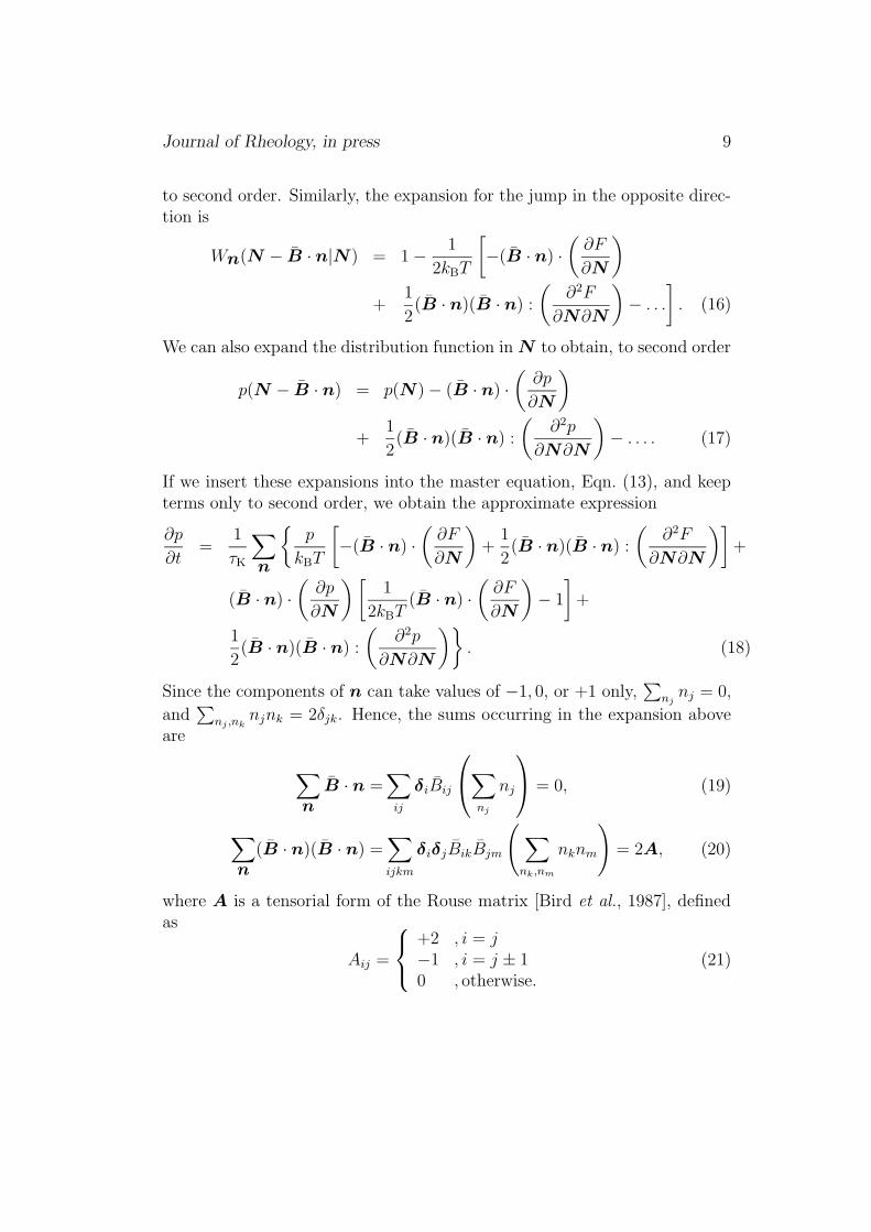
to second order. Similarly, the expansion for the jump in the opposite direc-tion is

Wn(N − B · n|N ) = 1 − 1

2kBT

[

−(B · n) ·(

∂F

∂N

)

+1

2(B · n)(B · n) :

(

∂2F

∂N∂N

)

− . . .

]

. (16)

We can also expand the distribution function in N to obtain, to second order

p(N − B · n) = p(N) − (B · n) ·(

∂p

∂N

)

+1

2(B · n)(B · n) :

(

∂2p

∂N∂N

)

− . . . . (17)

If we insert these expansions into the master equation, Eqn. (13), and keepterms only to second order, we obtain the approximate expression

∂p

∂t=

1

τK

∑

n

p

kBT

[

−(B · n) ·(

∂F

∂N

)

+1

2(B · n)(B · n) :

(

∂2F

∂N∂N

)]

+

(B · n) ·(

∂p

∂N

)[

1

2kBT(B · n) ·

(

∂F

∂N

)

− 1

]

+

1

2(B · n)(B · n) :

(

∂2p

∂N∂N

)

. (18)

Since the components of n can take values of −1, 0, or +1 only,∑

njnj = 0,

and∑

nj ,nknjnk = 2δjk. Hence, the sums occurring in the expansion above

are

∑

n

B · n =∑

ij

δiBij

∑

nj

nj

= 0, (19)

∑

n

(B · n)(B · n) =∑

ijkm

δiδjBikBjm

(

∑

nk,nm

nknm

)

= 2A, (20)

where A is a tensorial form of the Rouse matrix [Bird et al., 1987], definedas

Aij =

+2 , i = j−1 , i = j ± 10 , otherwise.

(21)

Journal of Rheology, in press 10

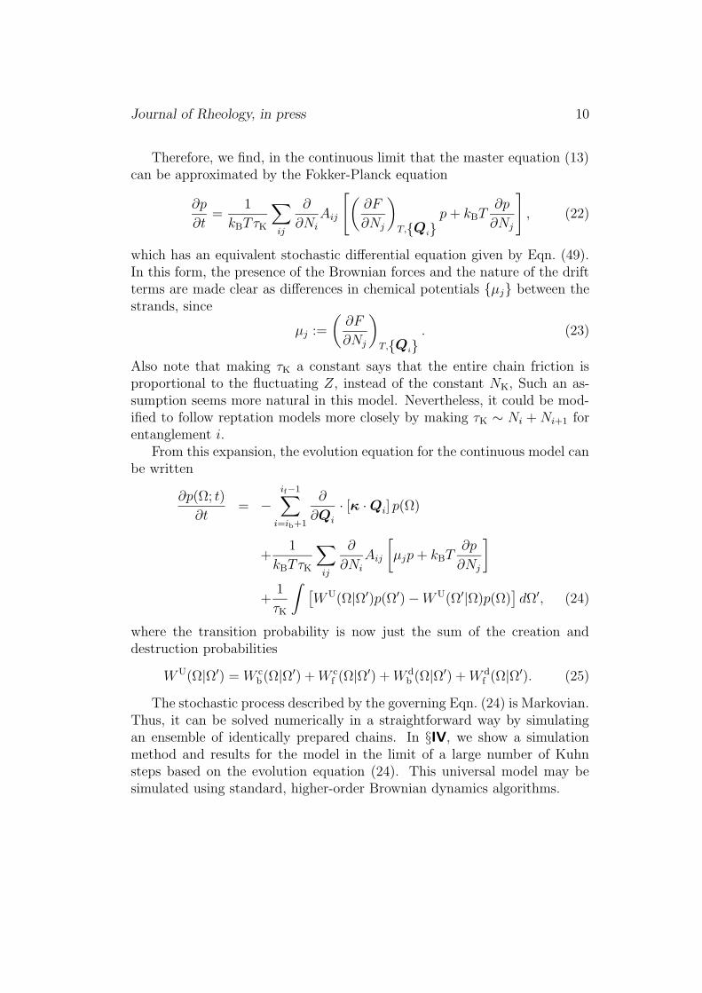
Therefore, we find, in the continuous limit that the master equation (13)can be approximated by the Fokker-Planck equation

∂p

∂t=

1

kBTτK

∑

ij

∂

∂Ni

Aij

[

(

∂F

∂Nj

)

T,Qip + kBT

∂p

∂Nj

]

, (22)

which has an equivalent stochastic differential equation given by Eqn. (49).In this form, the presence of the Brownian forces and the nature of the driftterms are made clear as differences in chemical potentials µj between thestrands, since

µj :=

(

∂F

∂Nj

)

T,Qi. (23)

Also note that making τK a constant says that the entire chain friction isproportional to the fluctuating Z, instead of the constant NK, Such an as-sumption seems more natural in this model. Nevertheless, it could be mod-ified to follow reptation models more closely by making τK ∼ Ni + Ni+1 forentanglement i.

From this expansion, the evolution equation for the continuous model canbe written

∂p(Ω; t)

∂t= −

if−1∑

i=ib+1

∂

∂Qi

· [κ · Qi] p(Ω)

+1

kBTτK

∑

ij

∂

∂Ni

Aij

[

µjp + kBT∂p

∂Nj

]

+1

τK

∫

[

WU(Ω|Ω′)p(Ω′) − WU(Ω′|Ω)p(Ω)]

dΩ′, (24)

where the transition probability is now just the sum of the creation anddestruction probabilities

WU(Ω|Ω′) = W cb(Ω|Ω′) + W c

f (Ω|Ω′) + W db (Ω|Ω′) + W d

f (Ω|Ω′). (25)

The stochastic process described by the governing Eqn. (24) is Markovian.Thus, it can be solved numerically in a straightforward way by simulatingan ensemble of identically prepared chains. In §IV, we show a simulationmethod and results for the model in the limit of a large number of Kuhnsteps based on the evolution equation (24). This universal model may besimulated using standard, higher-order Brownian dynamics algorithms.

Journal of Rheology, in press 11

II.D Stress tensor

The polymer contribution to the stress tensor is of the Kramers form

τ p = −n

if−1∑

j=ib+1

∑

N

∫ ∫ ∫

Qj

(

∂F

∂Qj

)

T,Ni

p(Qi, Niifib

; t)dQj, (26)

where n is the number density of polymer chains. Thus, for a given expressionof the free energy, stress predictions of the model are completely specified.The unentangled end strands of a chain do not contribute to the stress. Itis possible to show that this equation is that which arises in GENERIC[Ottinger and Grmela, 1997], and is guaranteed to satisfy the stress-opticrule. The complete continuous model is given by Eqs. (24), (25) and (26),and represents the first important result of this paper.

III Free Energy of a Chain

With the derivation in §II.B of the evolution equation Eqn. (4) (or for theuniversal limit, Eqn. (24) found in §II.C), the dynamical framework of themodel is now complete. Since a relation between chain configurations and themacroscopic stress has also been derived in §II.D, the only task remaining,in order to complete the model formulation, is to specify the free energies,FS(Q, N) and FE(N).

III.A Non-Universal Behavior

To find the free energy of the chain, we first require that the chain satisfy thestatistics of a Gaussian chain. Since the entanglements themselves define aprimitive path, this primitive path should represent a coarse-grained versionof the full chain. However, to prevent the chain from collapsing to a singleunentangled strand we place it in a chemical potential bath. However, thischemical potential is not placed at the ends of the chain like a Maxwelldemon. Instead, the bath is on the chemical potential conjugate to Z, notNi. If we call this chemical potential log β, we can include its effect by placingone such quantity in the free energy of each strand

FS(Q, N)

kBT=

3Q2

2Na2K

+3

2log(

2πN

3) + log β. (27)

Journal of Rheology, in press 12

By requiring that the model have the desired average number of Kuhn stepsper strand, we can (and do below) find a simple expression for β. We alsorequire an expression for the free energy of a dangling end. This expressionis not as important, and several expressions are possible. Here we pick themost convenient expression

FE(Q, N)

kBT= − log Ni + log β. (28)

If we plug Eqs. (27) and (28) into the expression for the chain free energy,Eqn. (2), then the Maxwell-Boltzmann relation, Eqn. (1) becomes

peq(Ni, Qi, Z) =δNK,

∑Zi=1 Ni

J

N1NZ

βZ×

Z−1∏

i=2

(

3

2πNi

)3/2

exp

[

− 3Q2i

2Nia2K

]

, (29)

where J is a normalization constant. We can integrate this expression overall Qi to find the distributions for Ni

peq(Ni, Z) =δNK,

∑Zi=1 Ni

J

N1NZ

βZ. (30)

If we sum this expression over all possible values of the Ni, we obtain thedistribution for Z

peq(Z) =(NK + 1)!

JβZ(Z + 1)!(NK − Z)!, Z ≥ 3. (31)

This is a binomial distribution. The expressions for Z=1,2 are

peq(Z = 1) =NK

Jβ, peq(Z = 2) =

(NK + 1)NK(NK − 1)

6Jβ2(32)

By summing over all possible values for Z, we find the normalization factor

J = (β + 1)

[

(

1 + β

β

)NK

− 1

]

+ NK

[

1 + 2β

6β2− 1 − NK

2β+

N2K(β − 1)

6β2

]

.(33)

Journal of Rheology, in press 13

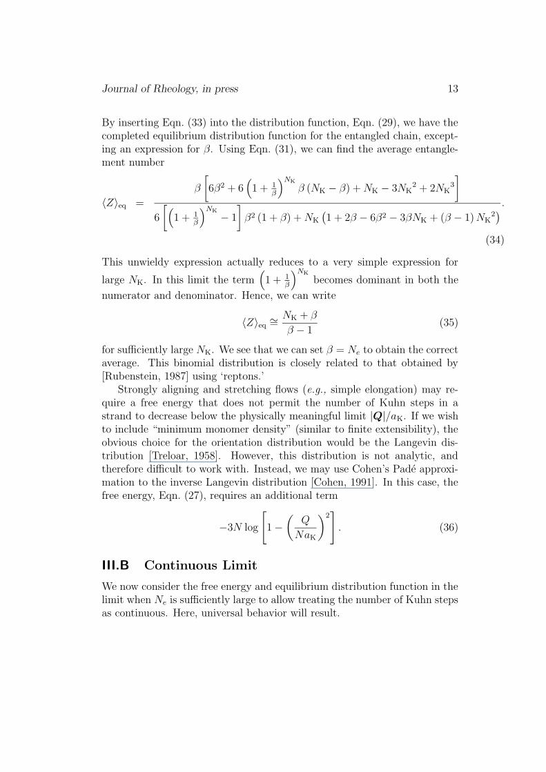
By inserting Eqn. (33) into the distribution function, Eqn. (29), we have thecompleted equilibrium distribution function for the entangled chain, except-ing an expression for β. Using Eqn. (31), we can find the average entangle-ment number

〈Z〉eq =

β

[

6β2 + 6(

1 + 1β

)NK

β (NK − β) + NK − 3NK2 + 2NK

3

]

6

[

(

1 + 1β

)NK

− 1

]

β2 (1 + β) + NK

(

1 + 2β − 6β2 − 3βNK + (β − 1) NK2)

.

(34)

This unwieldy expression actually reduces to a very simple expression for

large NK. In this limit the term(

1 + 1β

)NK

becomes dominant in both the

numerator and denominator. Hence, we can write

〈Z〉eq ∼= NK + β

β − 1(35)

for sufficiently large NK. We see that we can set β = Ne to obtain the correctaverage. This binomial distribution is closely related to that obtained by[Rubenstein, 1987] using ‘reptons.’

Strongly aligning and stretching flows (e.g., simple elongation) may re-quire a free energy that does not permit the number of Kuhn steps in astrand to decrease below the physically meaningful limit |Q|/aK. If we wishto include “minimum monomer density” (similar to finite extensibility), theobvious choice for the orientation distribution would be the Langevin dis-tribution [Treloar, 1958]. However, this distribution is not analytic, andtherefore difficult to work with. Instead, we may use Cohen’s Pade approxi-mation to the inverse Langevin distribution [Cohen, 1991]. In this case, thefree energy, Eqn. (27), requires an additional term

−3N log

[

1 −(

Q

NaK

)2]

. (36)

III.B Continuous Limit

We now consider the free energy and equilibrium distribution function in thelimit when Ne is sufficiently large to allow treating the number of Kuhn stepsas continuous. Here, universal behavior will result.

Journal of Rheology, in press 14

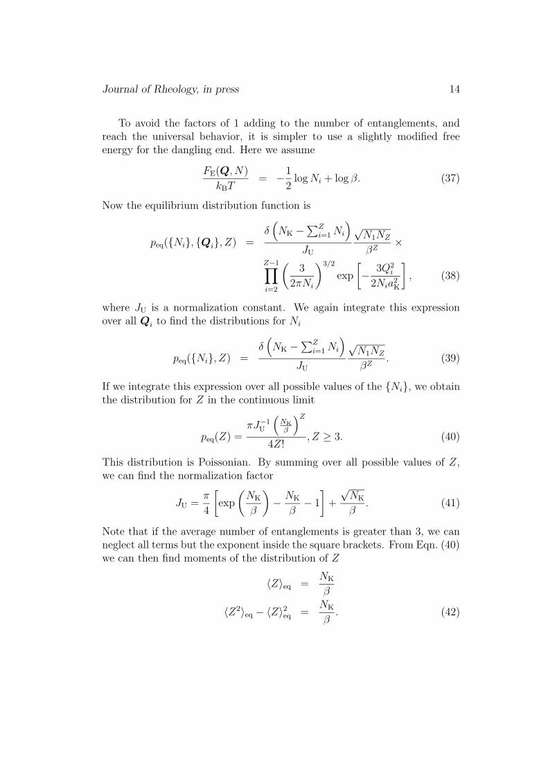
To avoid the factors of 1 adding to the number of entanglements, andreach the universal behavior, it is simpler to use a slightly modified freeenergy for the dangling end. Here we assume

FE(Q, N)

kBT= −1

2log Ni + log β. (37)

Now the equilibrium distribution function is

peq(Ni, Qi, Z) =δ(

NK −∑Z

i=1 Ni

)

JU

√N1NZ

βZ×

Z−1∏

i=2

(

3

2πNi

)3/2

exp

[

− 3Q2i

2Nia2K

]

, (38)

where JU is a normalization constant. We again integrate this expressionover all Qi to find the distributions for Ni

peq(Ni, Z) =δ(

NK −∑Zi=1 Ni

)

JU

√N1NZ

βZ. (39)

If we integrate this expression over all possible values of the Ni, we obtainthe distribution for Z in the continuous limit

peq(Z) =πJ−1

U

(

NK

β

)Z

4Z!, Z ≥ 3. (40)

This distribution is Poissonian. By summing over all possible values of Z,we can find the normalization factor

JU =π

4

[

exp

(

NK

β

)

− NK

β− 1

]

+

√NK

β. (41)

Note that if the average number of entanglements is greater than 3, we canneglect all terms but the exponent inside the square brackets. From Eqn. (40)we can then find moments of the distribution of Z

〈Z〉eq =NK

β

〈Z2〉eq − 〈Z〉2eq =NK

β. (42)

Journal of Rheology, in press 15

This tells us that if we set our chemical potential to be

β = Ne, (43)

we retrieve the correct average number of Kuhn steps per entangled strand.The moments in Eqn. (34) reduce to those in (42) in the limit of large Ne

and NK.With these expressions for the free energy, we suggest that the probability

of destruction of an entanglement at a free end is

W d(NE) =Ne

τe

√

3

NE

(44)

Detailed balance, Eqn. (12), yields

W c(QS, NS, NE) = pG(QS|NS)pS(NS|NE)wc(NE). (45)

where the last term on the right side is the probability that a strand of NE

Kuhn steps becomes entangled

wc(NE) =1

τe

√

3

NE

(NE − 2). (46)

The second term in the product of Eqn. (45) is the conditional probabilitythat such a newly entangling free end of NE steps puts NS steps in theentangled strand

pS(NS|NE) =1

NE − 2, (47)

which is uniform in NS. Finally, pG in Eqn. (45) is just the Gaussian distri-bution for a strand of NS Kuhn steps

pG(QS|NS) =

(

3

2πNS

)3/2

exp

[

− 3Q2S

2NSa2K

]

. (48)

IV Simulation Algorithm for Universal Be-

havior

From the equilibrium distribution of chain conformations, we can generate anensemble of chains having the proper initial statistics. To generate a singlechain we use the following procedure.

Journal of Rheology, in press 16

1. The number of strands Z is chosen from a Poisson distribution ac-cording to Eqn. (40) using a rejection method [Press et al., 1992]. Thisimplementation neglects the difference between the distribution for gen-eral Z, and those for Z = 1, 2. However, for all but lightly entangledchains, this approximation is not problematic.

2. By integrating Eqn. (39) over all possible values for N1, Ni+1,Ni+2,. . . ,NZ , we can obtain the joint distribution

peq(N2, . . . , Ni, Z) =exp(−NK/Ne)

NZe

(

NK −∑i

j=2 Nj

)Z−i+1

(Z − i + 1)!

from which we can obtain the conditional probability

peq(Ni|Nj, 2 ≤ j ≤ i − 1, Z) =(Z − i + 2)

(

NK −∑ij=2 Nj

)Z−i+1

(

NK −∑i−1

j=2 Nj

)Z−i+2.

Using the inverse method, we can then draw the number of Kuhn stepssuccessively for each strand, beginning with strand 2. A similar methodis then used to determine the distribution of Kuhn steps in the danglingends given the number of Kuhn steps in the entangled strands.

3. The distribution of strand orientations is found from the Gaussian dis-tribution for a given number of Kuhn steps, Eqn.(48) using the Box-Muller method [Press et al., 1992].

The resulting distributions agree with the statistics described in §III.The dynamics prescribed by Eqn. (24) is equivalent to Z stochastic dif-

ferential equations for the number of Kuhn steps in each strand; Z − 2 de-terministic equations for the affine deformation of the interior strands; andprobabilistic jump processes for the creation and destruction of entangle-ments. We handle the simulation of each of these processes in turn.

The stochastic differential equations equivalent to the Fokker-Planck-likeportion of Eqn. (24), namely Eqn. (22), for the Kuhn steps are

dNi =1

kBTτK

(µi+1 − 2µi + µi−1) dt

+

√

2

τK

(dWi−1 − dWi) , i = ib, . . . , if . (49)

Journal of Rheology, in press 17

In the above equation, we set dWi = 0 for i = ib − 1, µib−1 = µib , andµif+1 = µif . We integrate these equations over a small time-step ∆t, andapproximate the drift terms for the entangled strands semi-implicitly overthe time interval

Ni(t + ∆t) = Ni(t) −∆t

2kBTτK

∑

j

Aij

µj[Qj(t + ∆t), Nj(t + ∆t)]

+ µj[Qj(t), Nj(t)]

+

√

2

τK

∑

j

Bij∆Wj, i = ib+1, . . . , if−1, (50)

where ∆Wi(t) is a Wiener increment with zero mean, and variance ∆t. Theformulation in Eqn. (50) guarantees conservation of Kuhn steps, and helpsensure that the algorithm is stable, since the number of Kuhn steps cannotbecome negative. However, this expression represents Z coupled nonlinearalgebraic equations in the unknown Ni(t + ∆t), which cannot be solvedanalytically. Hence, we solve these by an iterative technique at every timestep. Inserting the chemical potential and rearranging Eqn. (50) yields

Ni −3∆t

2N2i

Q2i (t + ∆t) = fi(t) +

∆t

2

[

µi+1 + µ

i−1

]

,

where Ni ≡ Ni(t + ∆t), µi is the chemical potential of strand i found from

the previous iteration, and

fi(t) := Ni(t) −∆t

2kBTτK

∑

j

Aijµj[Nj(t),Qj(t)] +

√

2

τK

∑

j

Bij∆Wj. (51)

The initial value of µi is that from the beginning of the time step. At each

iteration, the above equation is cubic in the unknown Ni, which has a well-known analytic solution. When the iteration has converged, µ

i → µi(t+∆t),and Eqn. (50) is solved.

The algorithm is second order in time-step size for the strands, but moreimportantly, it is stable. It is also found to converge very quickly, for even asmall tolerance in the iteration steps.

Affine deformation of the interior strands is expressed by evolution equa-tion (3), which has the exact solution

Qi(t + ∆t) = E(t + ∆t, t) · Qi(t), i = ib+1, . . . , if−1, (52)

Journal of Rheology, in press 18

in which E(t, t′) is the finite strain tensor [Bird et al., 1987].Finally, creation and destruction of entanglements at the ends of the chain

are determined by Eqs.(44) and (45). The probability that a dangling endwith NE Kuhn steps is destroyed in a timestep is given by

Probability of destruction =Ne

τe

√

3

NE

∆t. (53)

The probability of creation is

Probability of creation =1

τe

√

3

NE

(NE − 2)∆t. (54)

If the strand is created, the number of Kuhn steps placed in the newly en-tangled strand is chosen uniformly between 1 and NE − 1. The remainingmonomers are placed in the dangling end. The placement of the new entan-glement is chosen from the Gaussian distribution given by Eqn.(48).

The above algorithm is performed on an ensemble of chains and averagesare taken over this ensemble. Such an algorithm provides a numerical esti-mate of averages taken over a probability density whose evolution is describedby Eqn. (24). This evolution equation should provide an excellent approxi-mation to the discrete model, Eqn. (4) when the number of Kuhn steps inthe chain is large. We have also made the algorithm dimensionless by pickinga characteristic length of

√NeaK, a characteristic time τK, and normalizing

all the Kuhn step numbers by Ne. Such a procedure eliminates NK, Ne, aK,and τe from the simulation, except for terms of NK/Ne, and some terms of1/Ne in Eqn. (54). However, for sufficiently large Ne, these latter terms canbe neglected. Here we choose Ne = 100 for numerical convenience, but theresults are not expected to be sensitive to the exact value.

The algorithm described is second-order in time step size for the Browniandynamics of the Kuhn steps, and exact for the evolution of the entanglementpositions, but first-order for creation and destruction. Most importantly, thealgorithm is stable for fairly large time step sizes, first order for a time-stepsize of at least ∆t ≤ 0.15τe, and has nearly zero slope in error.

V Results

In the shear simulations that are to follow, we use NK

Ne= 15. The ensemble

size is in most cases 5000 chains, and all simulations are found to converge

Journal of Rheology, in press 19

for a time step size of ∆t ∼= 0.1NeτK. To be safe, we use a time step sizehalf that large. Nonetheless, to calculate the stress for twice the longestrelaxation time requires only a couple of hours on a laptop for an ensembleof 5000.

In order to determine the phenomenological parameter τK for the systemconsidered, we relate it to the reptation time, τd, by means of Eqn. (6.19)of [Doi and Edwards, 1986]

τd =ζN3

Ka2K

π2NekBT=

N3K

π2Ne

τK, (55)

in which we have substituted ζ = kBTa2K

τK, the friction coefficient when the

test chain slips through an entanglement. However, these estimates for thelongest relaxation time neglect the effect of contour length fluctuations, whichare included here. Hence, we expect the longest relaxation time to be sig-nificantly smaller than τd, except for extremely long chains. We define thelongest relaxation time λ to be some fraction of τd

λ := c1τd, (56)

where c1 is a numerical coefficient of order unity or smaller. It remains to de-termine c1 which is obtained by comparing the simulated relaxation moduluswith linear viscoelastic experiments. If we perform a linear response calcu-lation at equilibrium, we can obtain a prediction for the relaxation modulusG(t)/3nkT 〈Z〉eq. When these simulation results are fit to a relaxation spec-trum, the longest relaxation time may be estimated, yielding a value for c1.A simulation of chains with 〈Z〉eq = 15 yielded an estimate of c1

∼= 0.2.For the following nonlinear calculations, we have also adopted a crude

variance reduction technique, which is helpful to reduce computation costsat low Deborah numbers. The control variates are the strand conformationsupon creation.

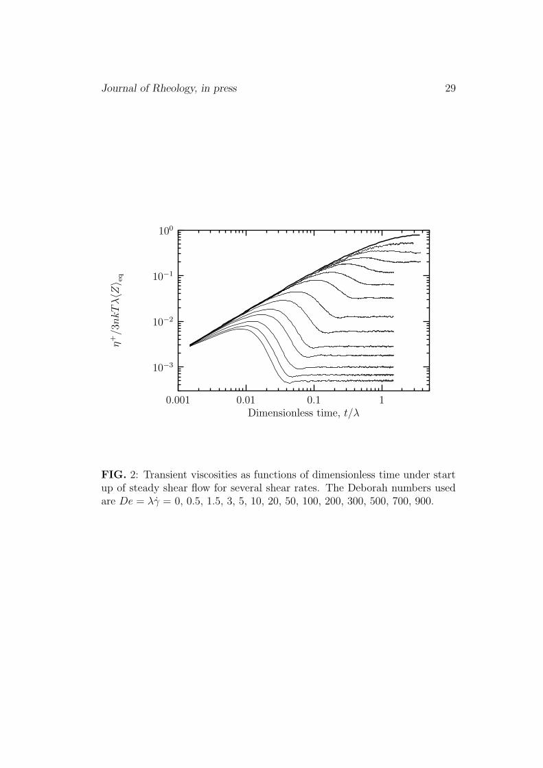
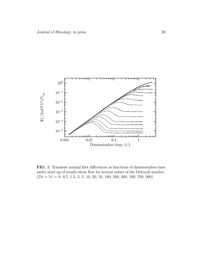
Figure 2 shows η+, the shear viscosity, as a function of time during in-ception of steady shear for several shear rates (expressed by the Deborahnumber for the flow, De := λγ). The curves appear very similar to the corre-sponding curves for the full-chain reptation model with fewer entanglements(see Figure 2 of [Hua et al., 1999]). The same trend is seen in Figure 3, wherewe repeat the plots in Figure 2, but for Ψ+

1 , the first normal stress difference.It is seen that the onset of overshoot for the normal stress occurs at a highershear rate than for the viscosity in agreement with experiments.

Journal of Rheology, in press 20

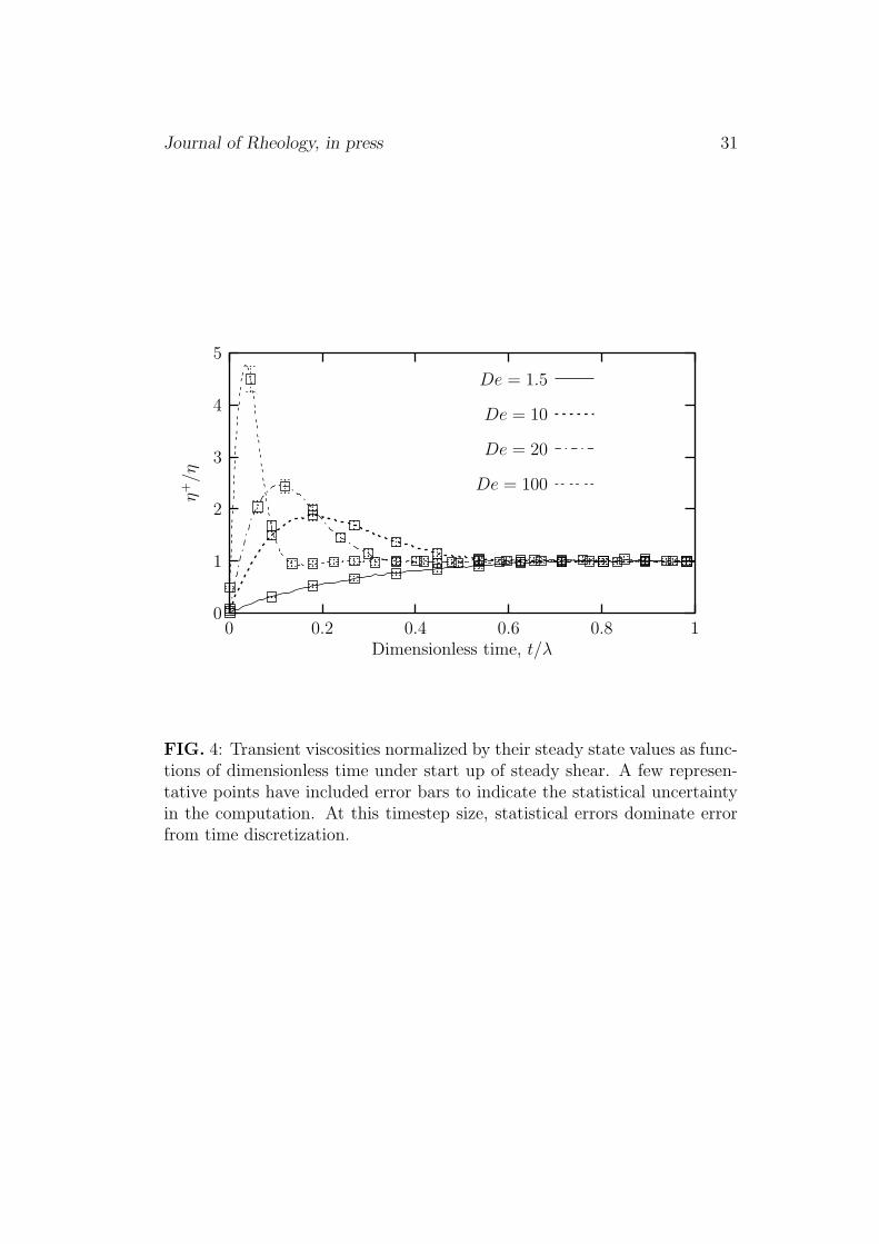
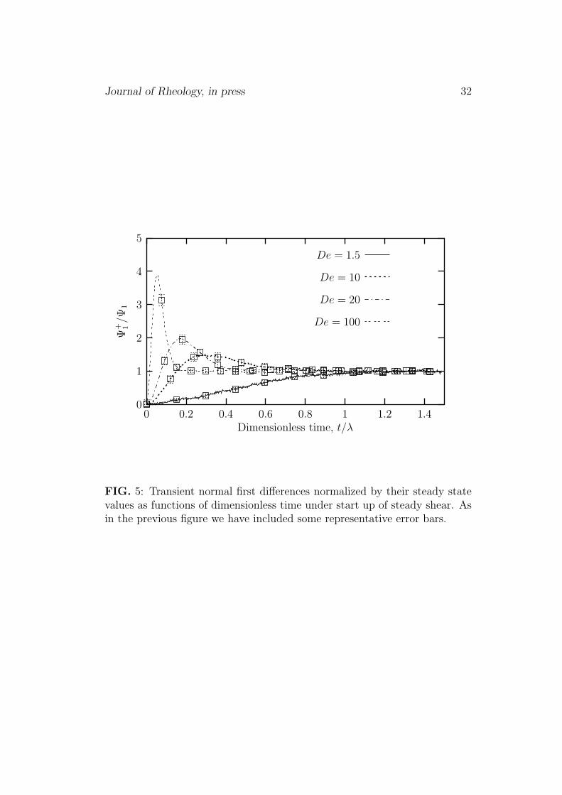
In Figures 4 and 5 we again plot the viscosity and first normal stress dif-ference respectively versus time for start up of steady shear at four differentshear rates. The plots are normalized by the steady state values in order tofocus on the magnitude of the overshoots in the transient phase. The full-chain reptation model overpredicts the magnitude of the stress overshoots.A similar trend may be evident here, although the number of entanglementsis larger. It is unlikely that constraint release will adjust these results suffi-ciently to give agreement with the data. The discrepancy may be related tothe assumption of affine deformation.

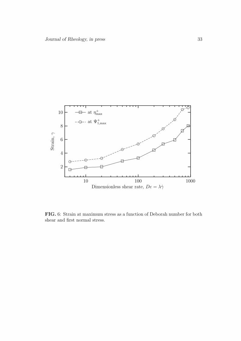
We can plot the strain at which the maximum in the overshoots occur.Figure 6 shows the strain at maximum stress for both shear and first normalstress differences. In qualitative agreement with data, the model shows aflat region at small De, and values that increase at larger strain rates. Theinitial values of 1.6 and 2.7 for shear and normal stresses, respectively, aresmaller than what is seen experimentally for more lightly entangled systems.However, the trends are similar.

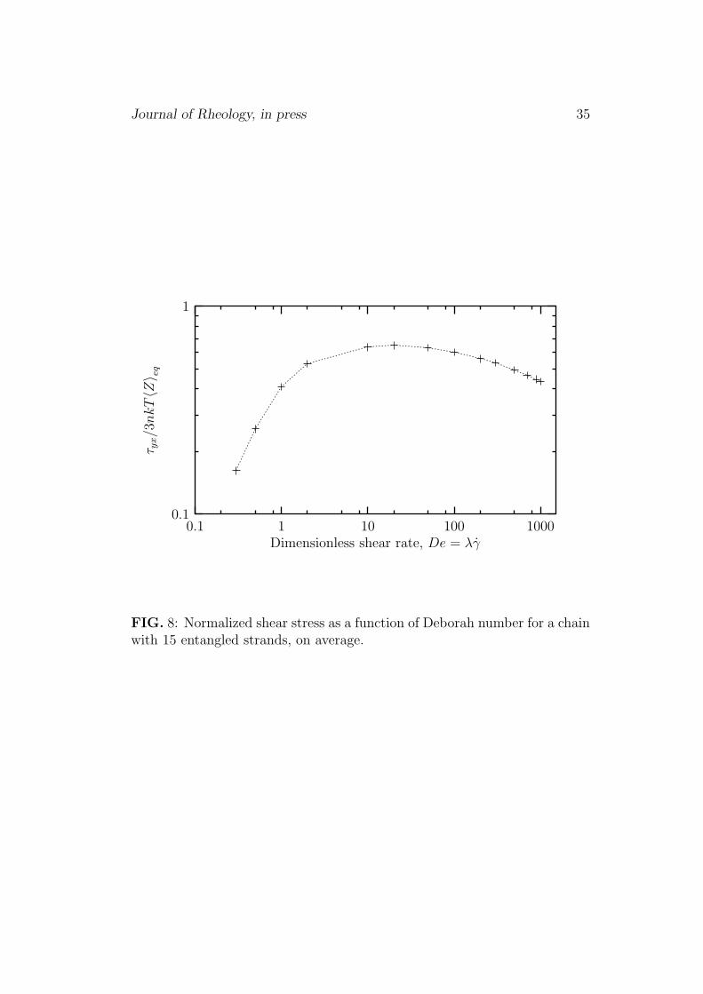
The steady state viscosity is shown as a function of shear rate in Figure 7.A fit of the power law behavior as predicted by the new model yields apower-law index of −0.142 ± 0.007. The full-chain reptation model predictsa maximum in the shear stress with shear rate, with or without constraintrelease. The slope observed here is very close to that observed for the tubemodel without constraint release. The shear stress is plotted as a function ofDeborah number in Figure 8. The maximum in this curve again emphasizesthe importance of convective constraint release at high shear rates.

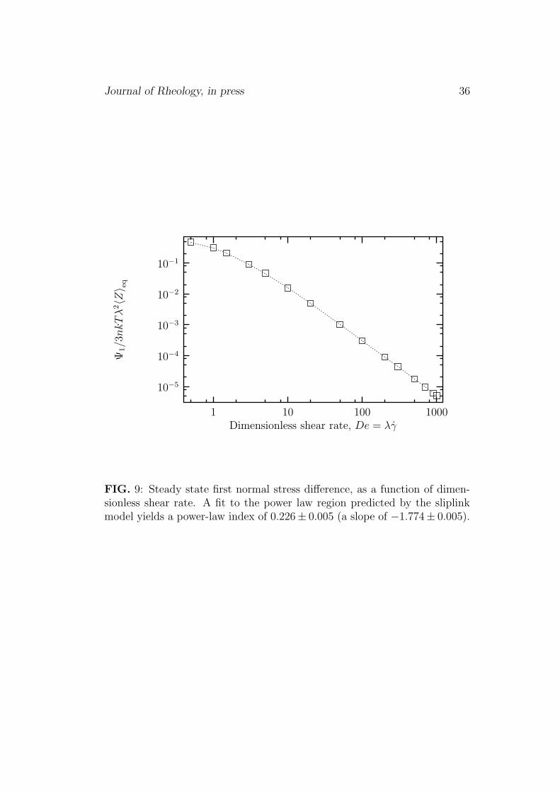
The analogous plot for the first normal stress difference is seen in Figure 9.Here, the power law slope of the curve for the new model gives a power-lawindex of 0.226 ± 0.005 (or slope of −1.774 ± 0.005), which is reasonable.

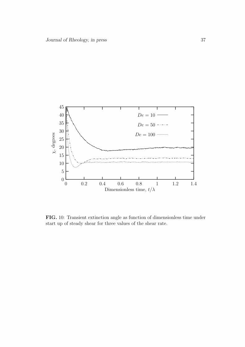
We also consider the transient extinction angle during start up of steadyshear. Figure 10 depicts χ+, the extinction angle for inception of steadyshear at three different shear rates, De = 10, 50, 100. It is seen that the χ+

curves exhibit an undershoot even at moderate shear rates. The shapes ofthese curves are reasonable, given what is known from the available data.

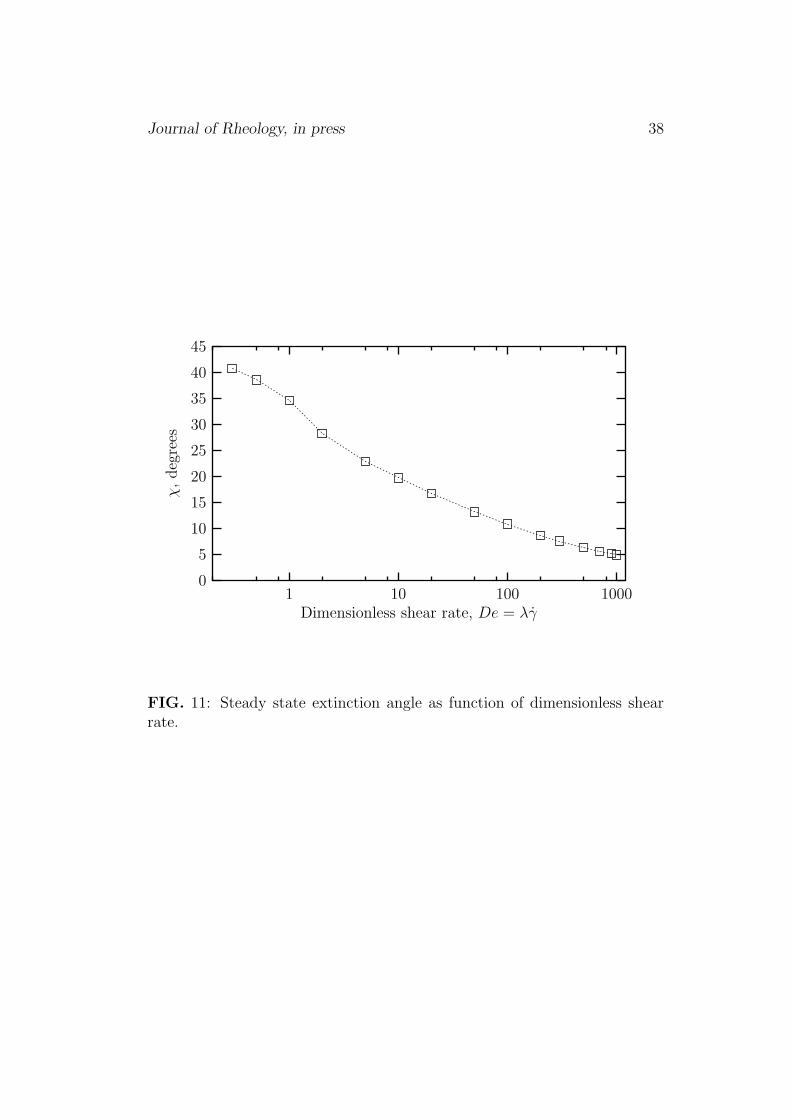
In Figure 11 we plot the steady state extinction angle as a function ofshear rate. With a steady state extinction angle of ∼ 5 for a very high shearrate of De = 1000, it is evident that the model predicts a non-zero value ofχ at steady state for all experimentally accessible shear rates and providesa reasonable description of the experimental data. This is an improvementover the full-chain reptation model, which predicts the steady state value of

Journal of Rheology, in press 21

χ to approach zero for high shear rates (see Figure 12 of [Hua et al., 1999]).Since entanglements are created only at the ends of the chain, flow can

decrease the number of entanglements rather dramatically for this imple-mentation of the model. Figure 12 shows the distribution of the number ofstrands in a chain at a Deborah number of 100. Although the distributionstill appears to be Poissonian, the average has dropped to approximately halfof its equilibrium value.

VI Conclusions

We have derived a novel full-chain temporary network model. Overall we cansummarize the evaluation of the model in inception of steady shear and steadystate shear, by noting that the steady state predictions are very encouraging.The results are comparable to those seen for a chain-in-a-tube simulationswithout constraint release [Hua and Schieber, 1998b]. Although the shearstress is a nonmonotonic function of shear rate as for tube models, at highshear rates the extinction angle is predicted to approach a non-zero plateau.Also, the transient results reveal too much overshoot for both the shear andnormal stresses, similar to the tube model.

The model proposes a new framework, where the Kuhn steps are a dy-namic variable, rather than a parameter [Schieber, 2000]. Within this frame-work, the physics implemented here are somewhat different from traditionaltube models. First, the entanglements are at discrete points along the chain,rather than smeared out in an average way, as with a tube. Secondly, en-tanglement spacing is not treated as a constant, but rather there exists adistribution of spacing which arises naturally from the free energy. Thisassumption was previously examined within the temporary network model[Neergaard, 2001]. In that work, stresses showed an excessive underdampedbehavior not seen here. Hence, at least for temporary networks, a distribu-tion of entanglement spacing improves the theoretical predictions. Thirdly,the friction experienced by the chain in its environment is located at theentanglements only, instead of at each monomer. Hence, the friction fluctu-ates with the number of entanglements. A similar approach is also taken ina simulation of a 3D network model on a more-detailed level of descriptionby [Masabuchi et al., 2001]. In that model the probability of entanglementcreation and destruction depends on the total number of entanglements ona chain—a global quantity. In that way, the fluctuations in Z are largely

Journal of Rheology, in press 22

suppressed. The framework here could be modified to allow the total fric-tion to remain constant, as it does in traditional reptation theories [Doi andEdwards, 1986], without resorting to an artificial suppression of fluctuationsin entanglement number.

Although the potential of the model has been demonstrated by consider-ation of its nonlinear flow behavior in §V, much improvement is still possible.We summarize here possible generalizations to the transient network model,using knowledge gleaned from the study of reptation models.

• The chain considered here is in a matrix of fixed obstacles. A chainin fluctuating obstacles—such as a polymer melt—will also undergoRouse-like motion, as first discussed by [de Gennes, 1975], and success-fully exploited by [Rubenstein and Colby, 1988] and [Likhtman andMcLeish, 2002]. The time-scale for the motions is determined not bythermal motion, but by the rate of ‘constraint release.’ These motionsare straightforward to include here as Brownian forces and ‘spring-like’forces of magnitude (∂F/∂Q)N,T on the entanglements. The time con-stant of such motion is determined by the timescale of the matrix. Inflows, such a constant should also include a term from entanglementdestruction caused by flow—so called ‘convective constraint release’[Ianniruberto and Marrucci, 2000; Marrucci, 1996]. Note that the mo-tions for this model are not ‘Rouse-like’, but actually Rouse. In otherwords, the evolution equation (24) requires additional terms of the type

−Z−1∑

i,j=2

Nea2K

kBTτCRij

Aij∂

∂Qi

·[

p

(

∂F

∂Qj

)

T,Nj

− kBT∂p

∂Qj

]

, (57)

where τCRij is a timescale for constraint release of strand connected to

entanglements i and j.

• Here we have considered only linear chains. However, branched andstar architectures are also possible. Star architectures are particularlyrelevant, since the activated process of arm retraction through contourlength fluctuations can be naturally studied. Branched chain architec-tures can be studied if one calculates the free energy of a branch pointtrapped between three sliplinks. Such a calculation is straightforward.

• As pointed out in §III, finite monomer density may also be employedby proper modification of the free energy, Eqn. (36). This effect isexpected to be important in extensional flows.

Journal of Rheology, in press 23

• Non-affine motion of the sliplinks is also possible. For example, [Mar-rucci et al., 2000] suggested that force balances between entanglementsmight be important to explain normal stresses quantitatively. Mostinteresting is the suggestion by [Rubenstein and Panyukov, 2002] toincorporate constrained dynamics of chains in lightly crosslinked sys-tems. This idea could be implemented here in an identical way. Theeffect is analogous to non-constant tube diameter in the language oftube models.

• The number of entanglements in the chain are decreased by the flow.Traditional tube theories assume that the number of entanglements isconstant during flow. Such an assumption could be implemented hereby imposing entanglements in the middle of the chain. The rate ofentanglement imposition would need to be equal to the rate at whichentanglements are swept off the end to keep the total number of entan-glements constant. This rate would then be closely related to the rateof convective constraint release.

Acknowledgments

J.N. would like to thank the Danish government for financial supportthrough the Technical University of Denmark (DTU).

J.D.S. would like to thank Professors M. Doi, T. Kawakatsu, and J. Taki-moto for useful discussions during a visit to Nagoya University funded bythe Doi Project, and for useful discussions with Professor Hans ChristianOttinger during a visit to ETH-Zurich.

References

Bird, R. B., C. F. Curtiss, R. C. Armstrong and O. Hassager, Dynamics of

Polymeric Liquids Vol. II: Kinetic Theory, Wiley-Interscience, New York,2nd edn. (1987).

Cohen, A., “A Pade approximant to the inverse Langevin function,” Rheol.Acta 30, 270–273 (1991).

de Gennes, P.-G., “Reptation of a polymer chain in the presence of fixedobstacles,” J. Chem. Phys. 55, 572–579 (1971).

Journal of Rheology, in press 24

de Gennes, P.-G., “Reptation of stars,” J.Phys.Paris 36, 1199–1203 (1975).

des Cloizeaux, J., “Double reptation vs. simple reptation in polymer melts,”J. Europhys. Lett. 5, 437–442 (1988).

Doi, M. and S. F. Edwards, “Dynamics of concentrated polymer systemspart 1. Brownian motions in the equilibrium state,” J. Chem. Soc. FaradayTrans. II 74, 1789–1800 (1978a).

Doi, M. and S. F. Edwards, “Dynamics of concentrated polymer systemspart 2. molecular motion under flow,” J. Chem. Soc. Faraday Trans. II 74,1802–1817 (1978b).

Doi, M. and S. F. Edwards, “Dynamics of concentrated polymer systemspart 3. the constitutive equation,” J. Chem. Soc. Faraday Trans. II 74,1818–1832 (1978c).

Doi, M. and S. F. Edwards, The Theory of Polymer Dynamics, ClarendonPress, Oxford (1986).

Fang, J., M. Kroger and H. C. Ottinger, “A thermodynamically admissiblereptation model for fast flows of entangled polymers ii. Model predictionsfor shear and extensional flows,” J. Rheol. 44, 1293–1317 (2000).

Gardiner, C. W., Handbook of Stochastic Methods for Physics, Chemistry

and the Natural Sciences, Springer-Verlag, Berlin, 2nd edn. (1982).

Hua, C. C. and J. D. Schieber, “Segment connectivity, chain-length breath-ing, segmental stretch, and constraint release in reptation models. I. The-ory and single-step strain predictions,” J. Chem. Phys. 109, 10018–10027(1998a).

Hua, C.-C. and J. D. Schieber, “Viscoelastic flow through fibrous media usingthe CONNFFESSIT approach,” J. Rheol. 42, 477–491 (1998b).

Hua, C. C., J. D. Schieber and D. C. Venerus, “Segment connectivity, chain-length breathing, segmental stretch, and constraint release in reptationmodels. II. Double-step strain predictions,” J. Chem. Phys. 109, 10028–10032 (1998).

Journal of Rheology, in press 25

Hua, C. C., J. D. Schieber and D. C. Venerus, “Segment connectivity, chain-length breathing, segmental stretch, and constraint release in reptationmodels. III. shear flows,” J. Rheol. 43, 701–717 (1999).

Ianniruberto, G. and G. Marrucci, “Convective orientation renewal in entan-gled polymer,” J. Non-Newtonian Fluid Mech. 95, 363–374 (2000).

Ketzmerick, R. and H. C. Ottinger, “Simulation of a non-Markovian processmodeling contour length fluctuation in the Doi-Edwards model,” Contin-uum Mech. Thermodyn. 1, 113–124 (1989).

Likhtman, A. and T. C. B. McLeish, “Quantitative theory for linear dynamicsof linear entangled polymers,” Macromolecules 00, 00—00 (2002).

Marrucci, G., “Dynamics of entanglements: a nonlinear model consistentwith the Cox-Merz rule,” J. Non-Newtonian Fluid Mech. 62, 279–289(1996).

Marrucci, G., F. Greco and G. Ianniruberto, “Simple strain measure forentangled polymers,” J. Rheol. 44, 845–854 (2000).

Masabuchi, Y., J.-I. Takimoto, K. Koyama, G. Ianniruberto, G. Marrucciand F. Greco, “Brownian simulations of a network of reptating primitivechains,” J. Chem. Phys. 115, 4387–4394 (2001).

Mead, D. W., R. G. Larson and M. Doi, “A molecular theory for fast flowsof entangled polymers,” Macromolecules 31, 7895–7914 (1998).

Neergaard, J., A Stochastic Approach to Modelling the Dynamics of Linear

Entangled Polymer Melts, Ph.D. thesis, Technical University of Denmark,Department of Chemical Engineering, Lyngby, Denmark (2001).

Neergaard, J., K. Park, D. C. Venerus and J. D. Schieber, “Exponentialshear flow of linear, entangled polymeric liquids,” J. Rheol. 44, 1043–1054(2000).

Ottinger, H. C., “A thermodynamically admissible reptation model for fastflows of entangled polymers,” J. Rheol. 43, 1461–1493 (1999).

Ottinger, H. C. and M. Grmela, “Dynamics and thermodynamics of complexfluids. II. Illustrations of a general formalism,” Phys. Rev. E 56, 6633–6655(1997).

Journal of Rheology, in press 26

Petruccione, F. and P. Biller, “A numerical stochastic approach to networktheories of polymeric fluids,” J. Chem. Phys. 89, 577–582 (1988).

Press, W. H., S. A. Teukolsky, W. T. Vetterling and B. P. Flannery, Nu-

merical Recipes in FORTRAN: The Art of Scientific Computing, 2nd ed.,Cambridge University Press, Cambridge, 2nd edn. (1992).

Rubenstein, M., “Discretized model of entangled-polymer dynamics,” Phys.Rev. Letters 59, 1946–1949 (1987).

Rubenstein, M. and R. Colby, “Self-consistent theory of polydisperse entan-gled polymers:Linear viscoelasticity of binary blends,” J. Chem. Phys. 89,5291–5306 (1988).

Rubenstein, M. and S. Panyukov, “Elasticity of polymer networks,” Macro-molecules 00, 000–000 (2002).

Schieber, J. D., “A full chain network model with sliplinks and binary con-straint release,” vol. 2, pp. 120–122, XIIIth International Congress on Rhe-ology (2000).

Treloar, L. R. G., The Physics of Rubber Elasticity, Clarendon Press, Oxford,2nd edn. (1958).

Tsenoglou, C., “Viscoelasticity of binary homopolymer blends,” Am. Chem.Soc. Polym. Preprints 28, 185 (1987).

Vrahopoulou, E. P. and A. J. McHugh, “A consideration of the Yamamotonetwork theory with non-Gaussian chain segments,” J. Rheol. 31, 371–384(1987).

Journal of Rheology, in press 27

Figure CaptionsFig. 1 Schematic of the dynamic variables in the model for a chain of 7

strands. The position of each of the Kuhn steps in the strands is indicatedalthough such information is averaged out in the model.

Fig. 2 Transient viscosities as functions of dimensionless time under startup of steady shear flow for several shear rates. The Deborah numbers usedare De = λγ = 0, 0.5, 1.5, 3, 5, 10, 20, 50, 100, 200, 300, 500, 700, 900.

Fig. 3 Transient normal first differences as functions of dimensionlesstime under start up of steady shear flow for several values of the Deborahnumber. (De = λγ = 0, 0.5, 1.5, 3, 5, 10, 20, 50, 100, 200, 300, 500, 700,900).

Fig. 4 Transient viscosities normalized by their steady state values asfunctions of dimensionless time under start up of steady shear. A few rep-resentative points have included error bars to indicate the statistical uncer-tainty in the computation. At this timestep size, statistical errors dominateerror from time discretization.

Fig. 5 Transient normal first differences normalized by their steady statevalues as functions of dimensionless time under start up of steady shear. Asin the previous figure we have included some representative error bars.

Fig. 7 Normalized steady state viscosity as function of dimensionlessshear rate. A fit to the power law region predicted by the sliplink modelyields a power-law index of −0.142 ± 0.007.

Fig. 8 Normalized shear stress as a function of Deborah number for achain with 15 entangled strands, on average.

Fig. 9 Steady state first normal stress difference, as a function of dimen-sionless shear rate. A fit to the power law region predicted by the sliplinkmodel yields a power-law index of 0.226± 0.005 (a slope of −1.774± 0.005).

Fig. 10 Transient extinction angle as function of dimensionless time understart up of steady shear for three values of the shear rate.

Fig. 11 Steady state extinction angle as function of dimensionless shearrate.

Fig. 12 The distribution of number of strands in a chain at equilibrium(line), and at steady state with a Deborah number of 100 (bars).

Journal of Rheology, in press 28

FIG. 1: Schematic of the dynamic variables in the model for a chain of 7strands. The position of each of the Kuhn steps in the strands is indicatedalthough such information is averaged out in the model.

Journal of Rheology, in press 29

Dimensionless time, t/λ

η+/3

nkT

λ〈Z

〉 eq

10.10.010.001

100

10−1

10−2

10−3

FIG. 2: Transient viscosities as functions of dimensionless time under startup of steady shear flow for several shear rates. The Deborah numbers usedare De = λγ = 0, 0.5, 1.5, 3, 5, 10, 20, 50, 100, 200, 300, 500, 700, 900.

Journal of Rheology, in press 30

Dimensionless time, t/λ

Ψ+ 1/3

nkT

λ2〈Z

〉 eq

10.10.010.001

100

10−1

10−2

10−3

10−4

10−5

FIG. 3: Transient normal first differences as functions of dimensionless timeunder start up of steady shear flow for several values of the Deborah number.(De = λγ = 0, 0.5, 1.5, 3, 5, 10, 20, 50, 100, 200, 300, 500, 700, 900).

Journal of Rheology, in press 31

De = 100

De = 20

De = 10

De = 1.5

Dimensionless time, t/λ

η+/η

10.80.60.40.20

5

4

3

2

1

0

FIG. 4: Transient viscosities normalized by their steady state values as func-tions of dimensionless time under start up of steady shear. A few represen-tative points have included error bars to indicate the statistical uncertaintyin the computation. At this timestep size, statistical errors dominate errorfrom time discretization.

Journal of Rheology, in press 32

De = 100

De = 20

De = 10

De = 1.5

Dimensionless time, t/λ

Ψ+ 1/Ψ

1

1.41.210.80.60.40.20

5

4

3

2

1

0

FIG. 5: Transient normal first differences normalized by their steady statevalues as functions of dimensionless time under start up of steady shear. Asin the previous figure we have included some representative error bars.

Journal of Rheology, in press 33

at Ψ+1,max

at η+max

Dimensionless shear rate, De = λγ

Str

ain,γ

100010010

10

8

6

4

2

FIG. 6: Strain at maximum stress as a function of Deborah number for bothshear and first normal stress.

Journal of Rheology, in press 34

Dimensionless shear rate, De = λγ

η/3

nkT

λ〈Z

〉 eq

1000100101

0.1

0.01

0.001

FIG. 7: Normalized steady state viscosity as function of dimensionless shearrate. A fit to the power law region predicted by the sliplink model yields apower-law index of −0.142 ± 0.007.

Journal of Rheology, in press 35

Dimensionless shear rate, De = λγ

τ yx/3

nkT〈Z

〉 eq

10001001010.1

1

0.1

FIG. 8: Normalized shear stress as a function of Deborah number for a chainwith 15 entangled strands, on average.

Journal of Rheology, in press 36

Dimensionless shear rate, De = λγ

Ψ1/3

nkT

λ2〈Z

〉 eq

1000100101

10−1

10−2

10−3

10−4

10−5

FIG. 9: Steady state first normal stress difference, as a function of dimen-sionless shear rate. A fit to the power law region predicted by the sliplinkmodel yields a power-law index of 0.226± 0.005 (a slope of −1.774± 0.005).

Journal of Rheology, in press 37

De = 100

De = 50

De = 10

Dimensionless time, t/λ

χ,deg

rees

1.41.210.80.60.40.20

45

40

35

30

25

20

15

10

5

0

FIG. 10: Transient extinction angle as function of dimensionless time understart up of steady shear for three values of the shear rate.

Journal of Rheology, in press 38

Dimensionless shear rate, De = λγ

χ,deg

rees

1000100101

45

40

35

30

25

20

15

10

5

0

FIG. 11: Steady state extinction angle as function of dimensionless shearrate.

Journal of Rheology, in press 39

equilibrium distribution

distribution at steady state shear

Number of strands in a chain, Z

p(Z

)

302520151050

0.18

0.16

0.14

0.12

0.1

0.08

0.06

0.04

0.02

0

FIG. 12: The distribution of number of strands in a chain at equilibrium(line), and at steady state with a Deborah number of 100 (bars).