Welcome message from author
This document is posted to help you gain knowledge. Please leave a comment to let me know what you think about it! Share it to your friends and learn new things together.
Transcript


ii
Acknowledgments
This thesis would not have been possible without the support of many people inmy life. Before I begin, I would like to take this opportunity to thank these peoplefor their support through my Bucknell career:
• Dr. L. Felipe Perrone, for his help and guidance throughout my career at Buck-nell. Felipe has mentored me in research and life since my freshman year. Thanksfor everything Felipe.
• Peg Cronin, for her excellent help and support during the writing process.Through my regular meeting with Peg I have learned to think more criticallyabout my own writing. Thanks Peg for teaching me so much about writing, andmaking the thesis writing process bearable, even fun at times.
• Andrew Hallagan (’11), for his collaboration on SAFE. Andrew’s project worksin harmony with my own and I have learned a great deal from Andrew throughour collaboration. Good luck after graduation Andy.
• Heather Burrell for her patience and support throughout the writing process,particularly during times of elevated stress and/or frustration. Thanks for al-ways being there for me.
• My family and friends who supported me throughout my thesis as well as mycareer at Bucknell.
iii
Contents
Abstract xi
I Introduction and Background 1
1 Introduction 2
1.1 Modeling . . . . . . . . . . . . . . . . . . . . . . . . . . . . . . . . . . 2
1.2 Computer Simulation . . . . . . . . . . . . . . . . . . . . . . . . . . . 3
1.3 Discrete-Event Simulation . . . . . . . . . . . . . . . . . . . . . . . . 4
1.4 Simulation Workflow . . . . . . . . . . . . . . . . . . . . . . . . . . . 5
1.5 Common Problems in Simulation Studies . . . . . . . . . . . . . . . . 6
1.6 Enhancing Usability and Credibility . . . . . . . . . . . . . . . . . . . 7
2 Design of Experiments 10
2.1 2k Factorial Experimental Design . . . . . . . . . . . . . . . . . . . . 10
2.2 mk Factorial Design . . . . . . . . . . . . . . . . . . . . . . . . . . . . 13

CONTENTS iv
2.3 mk−p Fractional Factorial Design . . . . . . . . . . . . . . . . . . . . 13
2.4 Latin Hypercube and Orthogonal Sampling . . . . . . . . . . . . . . . 15
3 Parallel Simulation Techniques 17
3.1 Fine-Grained Parallelism . . . . . . . . . . . . . . . . . . . . . . . . . 17
3.2 Coarse-Grained Parallelism . . . . . . . . . . . . . . . . . . . . . . . . 18
3.3 Multiple Replications in Parallel . . . . . . . . . . . . . . . . . . . . . 19
4 Previous Automation Tools 21
4.1 CostGlue . . . . . . . . . . . . . . . . . . . . . . . . . . . . . . . . . . 21
4.2 ns2measure & ANSWER . . . . . . . . . . . . . . . . . . . . . . . . . 22
4.3 Akaroa . . . . . . . . . . . . . . . . . . . . . . . . . . . . . . . . . . . 23
4.4 SWAN-Tools . . . . . . . . . . . . . . . . . . . . . . . . . . . . . . . . 24
4.5 James II . . . . . . . . . . . . . . . . . . . . . . . . . . . . . . . . . . 24
4.6 Lessons Learned . . . . . . . . . . . . . . . . . . . . . . . . . . . . . . 25
II SAFE 26
5 Architecture 27
5.1 The Experiment Execution Manager . . . . . . . . . . . . . . . . . . 28
5.1.1 Asynchronous / Event-Driven Architecture . . . . . . . . . . . 29
5.1.2 Dispatching Design Points . . . . . . . . . . . . . . . . . . . . 32
CONTENTS v
5.1.3 Web Manager . . . . . . . . . . . . . . . . . . . . . . . . . . . 34
5.2 simulation client . . . . . . . . . . . . . . . . . . . . . . . . . . . . . . 35
6 Languages 38
6.1 XML Technologies . . . . . . . . . . . . . . . . . . . . . . . . . . . . 38
6.2 Experiment Configuration . . . . . . . . . . . . . . . . . . . . . . . . 41
6.3 Experiment Description Language . . . . . . . . . . . . . . . . . . . . 41
6.4 Boolean Expression Objects . . . . . . . . . . . . . . . . . . . . . . . 43
6.5 Design Point Generation . . . . . . . . . . . . . . . . . . . . . . . . . 44
6.5.1 Backtracking Design Point Generation . . . . . . . . . . . . . 44
6.5.2 Linear Design Point Generation . . . . . . . . . . . . . . . . . 46
6.5.3 Design Point Construction . . . . . . . . . . . . . . . . . . . . 46
7 Inter-Process Communication 49
7.1 IPC Mechanisms . . . . . . . . . . . . . . . . . . . . . . . . . . . . . 49
7.1.1 Pipes . . . . . . . . . . . . . . . . . . . . . . . . . . . . . . . . 51
7.1.2 Network Sockets . . . . . . . . . . . . . . . . . . . . . . . . . 51
7.2 EEM ↔ Simulation Client . . . . . . . . . . . . . . . . . . . . . . . . 52
7.3 Simulator ↔ Simulation Client . . . . . . . . . . . . . . . . . . . . . 53
7.4 EEM ↔ Transient and Run Length Detector . . . . . . . . . . . . . . 56
8 Storing and Accessing Results 57

vi
8.1 Databases . . . . . . . . . . . . . . . . . . . . . . . . . . . . . . . . . 57
8.1.1 Theory . . . . . . . . . . . . . . . . . . . . . . . . . . . . . . . 57
8.1.2 Database Management Systems . . . . . . . . . . . . . . . . . 59
8.2 SAFE’s Database Schema . . . . . . . . . . . . . . . . . . . . . . . . 60
8.3 Querying For Results . . . . . . . . . . . . . . . . . . . . . . . . . . . 62
III Applications and Conclusions 66
9 Applications 67
9.1 Case Study: A Custom Simulator . . . . . . . . . . . . . . . . . . . . 67
9.2 Case Study: ns-3 . . . . . . . . . . . . . . . . . . . . . . . . . . . . . 70
9.2.1 ns-3 Architecture . . . . . . . . . . . . . . . . . . . . . . . . . 70
9.2.2 ns-3 Simulation Client . . . . . . . . . . . . . . . . . . . . . . 71
10 Conclusions & Future Work 73
IV Appendices 80
A Polling Queues Example XML Configuration 81
B Example Experiment Configuration File 83
C Example Cheetah Template 85

vii
List of Tables
2.1 23 Factorial Design example. . . . . . . . . . . . . . . . . . . . . . . . 12
2.2 24−1 Fractional Factorial Design example. . . . . . . . . . . . . . . . . 15
6.1 Application specific subsets of factorial designs. . . . . . . . . . . . . 42

viii
List of Figures
2.1 Examples of different response surfaces. . . . . . . . . . . . . . . . . . 11
2.2 Example of the effect of granularity in experimental design. . . . . . . 14
2.3 An example of a Latin Square. . . . . . . . . . . . . . . . . . . . . . . 15
2.4 An example of Orthogonal Sampling. . . . . . . . . . . . . . . . . . . 16
3.1 Multi-processor speedup as a result of Amdahl’s law. . . . . . . . . . 19
5.1 Overview of the architecture of SAFE. . . . . . . . . . . . . . . . . . 28
5.2 Transient and run length detection processes interactions. . . . . . . . 30
5.3 Benefits of the reactor design pattern. . . . . . . . . . . . . . . . . . . 32
7.1 SAFE IPC architecture . . . . . . . . . . . . . . . . . . . . . . . . . . 50
7.2 Protocol for EEM/simulation client communication. . . . . . . . . . . 54
8.1 An example of database normalization. . . . . . . . . . . . . . . . . . 58
8.2 SAFE database schema. . . . . . . . . . . . . . . . . . . . . . . . . . 61
8.3 A visual depiction of the function f . . . . . . . . . . . . . . . . . . . 64

ix
9.1 An example of a polling queues system. . . . . . . . . . . . . . . . . . 68

x
Code Listings
6.1 An example XML Element. . . . . . . . . . . . . . . . . . . . . . . . 39
6.2 An example XML Element with an attribute. . . . . . . . . . . . . . 39
6.3 Nesting XML elements. . . . . . . . . . . . . . . . . . . . . . . . . . . 39
6.4 An example HTML document. . . . . . . . . . . . . . . . . . . . . . . 40
6.5 An example boolean expression object. . . . . . . . . . . . . . . . . . 44
6.6 Pseudocode for the backtracking design point generation algorithm. . 45
6.7 Pseudocode for the linear design point generation algorithm. . . . . . 46
8.1 A simple SQL SELECT statement . . . . . . . . . . . . . . . . . . . . . 59
8.2 Example of a SQL JOIN statement. . . . . . . . . . . . . . . . . . . . 60
8.3 SQL to query for a specific design point. . . . . . . . . . . . . . . . . 63

xi
Abstract
Simulation is an important resource for researchers in diverse fields. However, manyresearchers have found flaws in the methodology of published simulation studies andhave described the state of the simulation community as being in a crisis of credibility.This work describes the project of the Simulation Automation Framework for Exper-iments (SAFE), which addresses the issues that undermine credibility by automatingthe workflow in the execution of simulation studies. Automation reduces the numberof opportunities for users to introduce error in the scientific process thereby improvingthe credibility of the final results. Automation also eases the job of simulation usersand allows them to focus on the design of models and the analysis of results ratherthan on the complexities of the workflow.

Part I
Introduction and Background
1

2
Chapter 1
Introduction
Computer simulation is a valuable tool to people in many disciplines. This thesisdevelops a framework which aids simulation users in conducting their simulationstudies to ensure their results are accurate and reported properly. This work is bestunderstood with a background in computer modeling and simulation, as well as propersimulation methodology.
1.1 Modeling
In numerous applications ranging from engineering to the natural sciences to businessapplications, people seek to quantify the behavior of different real world processes andphenomena. When such a process or phenomenon is studied scientifically, it is called asystem. Assumptions are often made about the behavior of these systems which allowfor mathematical and scientific analysis. These assumptions comprise a model andare composed of mathematical or logical descriptions of the behavior of the system.[26]
Models are coupled with performance metrics which are used to quantify differentaspects of the behavior of a system. Models logically or mathematically relate metricswith input parameters called factors. The specific value given to a factor is called alevel. For example, when investigating a vehicular traffic system, the rate with whichcars arrive at a traffic light is a factor, while the numeric value of 10 cars per minute is

CHAPTER 1. INTRODUCTION 3
a level. Additionally, a model can be composed of many different sub-models whichthemselves describe the behavior of a smaller or simpler sub-system.
If a system or model is simple enough, mathematical analysis can be used toexplicitly solve for the value of different performance metrics. These solutions areknown as analytic solutions, and are the ideal way to quantify the behavior of thesystem under investigation. Using an analytic solution, one can more easily isolateeffects of different factors and find optimal factor-level combinations. These resultscan inform scientific developments as well as engineering and business decisions.
Solving for performance metrics analytically can be challenging, if not impossible,for more sophisticated and complex models. In such cases, engineers often study thesystem by simulating the behavior of the system using computers. In the absenceof an analytic solution, simulation can be employed to investigate the system undermany different sets of inputs.
1.2 Computer Simulation
Traditionally, real world experiments are conducted to test how systems behave underdifferent circumstances. Often times such experiments can be expensive, time con-suming, dangerous, or hard to observe. With modern computers and software, thesesystems can be evaluated using computer simulations. Simulation results, similar toanalytic solutions, can also be used to inform scientific advancements, engineering de-sign decisions, or business strategies. Further, simulations can sometimes be executedfaster than real time, helping to provide insight into future events or phenomenon.
A discipline which enjoys extensive use of simulation is the field of computer net-works. Take, for example, a researcher developing new wireless networking protocolsfor vehicles traveling at high speeds on roads and interstates. After developing sucha protocol, the researcher would want to evaluate its performance. Testing such aprotocol can be very costly, particularly when investigating how the network will farewith hundreds of vehicles traveling at high speeds over great geographic distances.In such a case, testing these new protocols using computer simulation can reducethe cost of testing and reduce development time. This is just one example of howsimulation allows for a more efficient engineering process.
Another application of computer simulation is in molecular biology. A project

CHAPTER 1. INTRODUCTION 4
called Folding@Home, uses computer simulation to investigate how proteins fold. TheFolding@Home project distributes simulation execution across volunteer computersthroughout the world to accelerate computationally expensive simulations. The resultsof these simulations are used to understand the development of many diseases suchas Alzheimer’s, ALS, and many cancers. [14]
With advancements in computer hardware over the last 50 years, computer simu-lation has become an increasingly powerful tool in science and engineering. Computersimulation has aided researchers in developing many of the technologies and businessstrategies that power our society today. As computer hardware continues to improve,simulation will become an even more powerful tool for people in a wide array of dis-ciplines and will play a critical role in future scientific developments, particularly asengineered systems become increasingly complex.
1.3 Discrete-Event Simulation
There are many ways to create a model in computer software. One such paradigmoften used to investigate time-varied systems is called Discrete-Event Simulation.In such simulations, the system is described and modeled through a chronologicalsequence of events. These events drive the behavior of the simulated system.
In a discrete-event simulation, the simulator maintains a simulation clock whichkeeps track of time in the simulated environment. Events which change the internalstate of the simulation are scheduled on the event list or event queue. During theexecution of an event, new events can be added to the events list. When an event isfinished processing, the simulation clock is advanced to the next event in simulatedtime. [13]
Discrete-event simulation is often used to investigate systems with random behav-ior, known as stochastic processes. The simulation of stochastic processes requiresthe generation of random numbers using a Pseudo-Random Number Genera-tor (PRNG), which produce a deterministic stream of numbers which appears tobe truly random. A PRNG must be seeded with a starting value, which is used ina mathematical algorithm that produces the subsequent values sequence. The samestream is recreated time after time with the same starting PRNG seed. Simulationsof stochastic processes which employ PRNGs to model their behavior are said to bestochastic simulators. [26]

CHAPTER 1. INTRODUCTION 5
A classic application of discrete-event simulation lies in queueing theory, whichis a well-established field of Operations Research. An example of an application ofqueueing theory is the study of lines in a shopping mall store. Neither the rate withwhich customers enter the queue nor the amount of time it takes for the cashierto check a customer out are constant, or deterministic. One can, however, assumethat these times are described by random variables and construct a discrete-eventsimulation to produce estimates of the average time a customer waits in line. In thiscase, the probability distribution of arrivals is a factor, and distribution itself, sayPoisson, is a level. The parameter of the random distribution, in the case of Poisson,λ, is also a level. The simulation model uses these levels for the associated factorsto schedule events such as a new customer entering a line and a cashier finishingchecking someone out.
1.4 Simulation Workflow
Once a computer simulation has been built, simulations can be run on many differentinputs. Simulators can therefore be used to conduct simulation experiments, inwhich the factors of the simulation are varied to investigate their effect on performancemetrics. Each unique input set of factors and associated levels in such an experimentis called an experimental design point. For example, a design point in the contextof a shopping mall store line is a complete set of levels for all the factors in the model,such as customer arrival rate and service rates.
A simulation experiment is composed of a set of design points to run. The actof choosing the particular set of design points to explore is called experimentaldesign. There are many experimental design techniques which users can employ tounderstand the effect of different factors on the performance metrics with less timespent in simulation execution. These techniques seek to constrain the experimentaldesign space, or the set of design points which are executed during the experiment’sexecution. Several of these techniques are described in more detail in Section 2.
Once the experimental design space is defined, one can start to execute simulationsto collect data. When using a stochastic simulator, it is best to run many simula-tions for each design point, each with a different PRNG seed and to compute averages,which are point estimates of the metrics collected. This ensures that results are notbiased by a particular stream of random numbers. Using the samples of these metricsand a chosen confidence level, one can compute confidence intervals, which give

CHAPTER 1. INTRODUCTION 6
a better estimate of the true value of the corresponding metrics.
The results obtained from the simulation runs may be saved in persistent storageto be analyzed upon the completion of the simulation experiment. The analysis of thisbody of data may test hypotheses or lead to conclusions about the system. Simulationresults are analyzed using many different statistical techniques.
There are many complexities associated with running an experimental simulationstudy. The aforementioned steps must be followed very carefully, and furthermore,one must take great care in reporting results. Just as in any other scientific process,simulation results must be reproducible and independently verifiable. Simulation usersmust therefore take precaution in reporting not only their results properly, but alsodetails of their experimental process so that an independent third party can replicatetheir results. When proper simulation workflow is put in practice, and experimentalmethodology and results are reported properly, a simulation study is credible.
1.5 Common Problems in Simulation Studies
Conducting a complete and thorough simulation experiment is an extensive process.There are countless opportunities for a user to make a mistake in the proper simulationworkflow. Many researchers [25, 28] have shown that these mistakes in proper simula-tion workflow lead to credibility issues. Furthermore, if the experimental methodologyis not reported accurately such that others can reproduce the experiment, the credi-bility of the results are compromised even if a simulation study is conducted properly.
Once simulation results have been collected, proper statistical methods need to beapplied to ensure that the statistics for the experiment accurately portray the results.Often times simulation users make naıve assumptions in their statistical analysis andmethodology which can lead to biased results. For example, users often assume thattheir results are Independent and Identically Distributed (IID), which allowsthem to use simple, standard formulas to calculate the mean and variance. It is notalways the case though that the samples are IID, and consequently, the reportedresults are often biased. [25]
Just as in any other statistical study, it is best to observe many observations ina sample to estimate different values more accurately. Consequently, in simulationexperiments it is best to run many simulations with different PRNG seeds to collect

CHAPTER 1. INTRODUCTION 7
many observation. Managing the results from hundreds to thousands of simulationscan be a daunting task. Furthermore, particularly in large experiments, a great dealof time can be spent running these simulations and managing their results. Onlyrunning a single simulation run for each design point is a very common mistake insimulation methodology seen in past and current literature [25].
Another common oversight in the analysis of simulation results is the lack ofcomputed confidence intervals. Simulations are a means to estimate certain populationstatistics for complex systems, and it is important in any statistical study to reportthe confidence of computed results. This problem is compounded in the case in whicha single simulation is executed per design point, and there is a single statistical sample.To ensure highly credible results, many simulation runs should be executed per designpoint, and the associated confidence interval should be reported with any statistics.
Simulation users often also forget to consider the transient or “warm up period”of a discrete-event simulation. Many of the initial results collected during the tran-sient are biased as the system approaches its steady state, which is most often whatsimulation users are most interested in studying. Therefore, the results collected dur-ing the transient should be discarded. This process is called data deletion, and isimportant to ensure that results are not biased. In network simulation, many stud-ies do not include data deletion, and those which do rely on arbitrary choices forthe length of the transient. According to Kurkowski et al. [25], the vast majority ofthe past and current literature using simulation to study Mobile Ad-Hoc Networks(MANETs) do not include any discussion of data deletion.
These problems in simulation workflow and analysis are further compounded byimproper reporting of experimental results and methodology in many simulation stud-ies. This has led Pawlikowski [29] to describe the current state of the network simu-lation community as a “crisis of credibility.”
1.6 Enhancing Usability and Credibility
Kurkowski et al. [25] explained that many of the steps necessary in proper simulationmethodology and statistical analysis are often skipped or conducted carelessly, therebycompromising the credibility of the results. Many of these steps in proper simulationworkflow can be automated through computer software automation tools to ensurethat results have a higher level of credibility. Perrone et al. [30] claimed that “The level

CHAPTER 1. INTRODUCTION 8
of complexity of rigorous simulation methodology requires more from [the simulationuser] than they are capable of handling without additional support from software tools.”
Mistakes in statistical analysis can be easily avoided through the use of softwaretools. Statistically inclined simulation developers can develop tools which walk asimulation user through all of the steps in proper statistical analysis. In this manner,all statistical results which the tools help the user to discover are ensured to be correct.For example, tools can ensure that confidence intervals are always provided for eachof the metric estimators. These tools can be extended to help users generate figuresensuring all axes are labeled, and confidence intervals are plotted.
Large simulation studies can include thousands of simulations which need to beexecuted. Such simulation studies can take thousands of processor hours to execute.To accelerate this process, independent simulations can be executed concurrently onmany processors on different physical computers. While this can reduce the simula-tion time, it also incurs more administrative overhead to partition the simulationsto run on many processors and aggregate results. Furthermore, this process intro-duces opportunities for the human user to compromise the integrity of their results.Automation tools can be used to manage the execution of simulation runs across anetwork of computers to reduce simulation time.
Automation tools ensure the credibility of simulation results while easing thesimulation workflow. This allows users to focus their efforts on modeling the system orunderstanding results instead of managing simulation execution. Computer simulationautomation tools make computer simulation more valuable to the research community.My thesis is thus:
Thesis StatementThe current state of the simulation community has been described as
a crisis of credibility. Automation tools address this issue by automatingthe processes in which common mistakes are made to ensure the credi-bility of results. Furthermore, automation tools can ease the simulationworkflow for users to allow them to focus on their science instead of thesimulation workflow. I have developed a framework which can be usedto automate many of the requisite steps in proper simulation workflow,thereby ensuring the credibility of collected results. This framework rep-resents a significant contribution to the simulation community which willhelp users produce more credible results.

CHAPTER 1. INTRODUCTION 9
This thesis is organized as follows. The remainder of Part I, discusses backgroundinformation relevant to my project. Part II describes the Simulation AutomationFramework for Experiments (SAFE), which represents my main contribution. Part III,looks at applications of SAFE and concludes the thesis.
Chapter Summary
Computer simulation is a valuable tool in many fields. To use a simulator properlyrequires careful attention to detail when conducting a simulation experiment. Whenusers are not careful, their results can easily be compromised, leading to results whichare not credible. To fully realize the utility of computer simulations, automation toolsare required to guide a user through the steps in proper simulation workflow toensure credible results. Chapter 2 describes several ways in which experiments can bedesigned to investigate relationships between performance metrics and factors.

10
Chapter 2
Design of Experiments
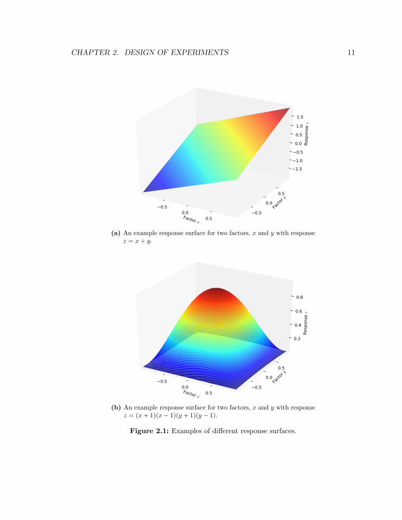
Simulation experiments are often conducted to evaluate relationships between factorsand performance metrics, sometimes called responses. The set of responses for manydesign points is known as the response surface. Response surfaces can take onmany shapes and forms as can be seen, for example, in Figure 2.1. Experimentscan be designed to investigate relationships between factors and their effect on aresponse surfaces. Many experimental design techniques exist to help users evaluatethe differences in responses from different factors. These techniques can reduce thenumber of simulations needed to understand these relationships.
2.1 2k Factorial Experimental Design
A simple technique often used to evaluate which factors have the largest effect onthe response is the 2k factorial experimental design. In this design, a low and a highlevel are chosen for each factor and permuted to compute all of the design points inthe experiment. These low and high values are often coded +1 and −1 respectively.An example of a 2k factorial design with 3 factors can be seen in Table 2.1. In a 2k
factorial design, there are 2k design points in the experiment where k is the numberof factors under investigation.
Using this experimental design technique, one can isolate which factors play thelargest role in the response. For example, to calculate the effect of factor 1, denoted
CHAPTER 2. DESIGN OF EXPERIMENTS 11
Factor x
0.50.0
0.5
Facto
r y
0.5
0.0
0.5
Resp
onse
z
1.5
1.0
0.5
0.0
0.5
1.0
1.5
(a) An example response surface for two factors, x and y with responsez = x + y.
Factor x
0.50.0
0.5
Facto
r y
0.5
0.0
0.5
Resp
onse
z
0.2
0.4
0.6
0.8
(b) An example response surface for two factors, x and y with responsez = (x + 1)(x− 1)(y + 1)(y − 1).
Figure 2.1: Examples of different response surfaces.
CHAPTER 2. DESIGN OF EXPERIMENTS 12
Design Point X1 X2 X3 Response1 −1 −1 −1 R1
2 +1 −1 −1 R2
3 −1 +1 −1 R3
4 +1 +1 −1 R4
5 −1 −1 +1 R5
6 +1 −1 +1 R6
7 −1 +1 +1 R7
8 +1 +1 +1 R8
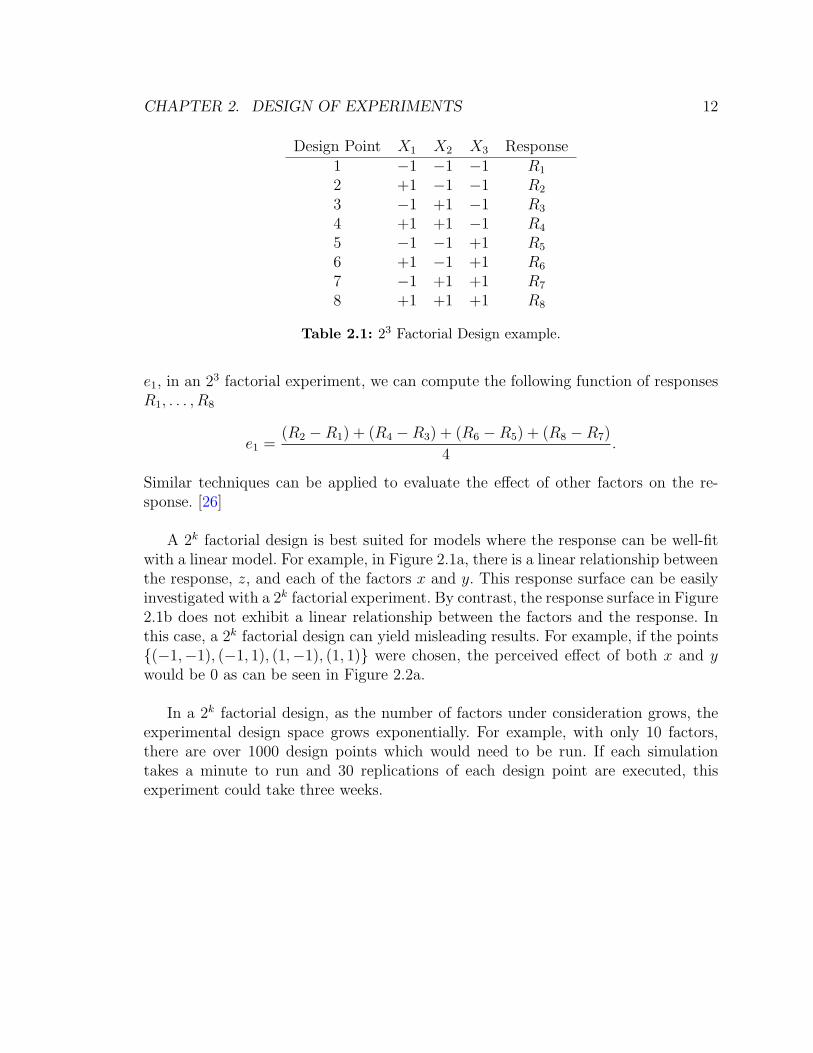
Table 2.1: 23 Factorial Design example.
e1, in an 23 factorial experiment, we can compute the following function of responsesR1, . . . , R8
e1 =(R2 −R1) + (R4 −R3) + (R6 −R5) + (R8 −R7)
4.
Similar techniques can be applied to evaluate the effect of other factors on the re-sponse. [26]
A 2k factorial design is best suited for models where the response can be well-fitwith a linear model. For example, in Figure 2.1a, there is a linear relationship betweenthe response, z, and each of the factors x and y. This response surface can be easilyinvestigated with a 2k factorial experiment. By contrast, the response surface in Figure2.1b does not exhibit a linear relationship between the factors and the response. Inthis case, a 2k factorial design can yield misleading results. For example, if the points{(−1,−1), (−1, 1), (1,−1), (1, 1)} were chosen, the perceived effect of both x and ywould be 0 as can be seen in Figure 2.2a.
In a 2k factorial design, as the number of factors under consideration grows, theexperimental design space grows exponentially. For example, with only 10 factors,there are over 1000 design points which would need to be run. If each simulationtakes a minute to run and 30 replications of each design point are executed, thisexperiment could take three weeks.

CHAPTER 2. DESIGN OF EXPERIMENTS 13
2.2 mk Factorial Design
A natural extension to the 2k factorial design is what is known as an mk factorialdesign. In this case, m levels are chosen for each factor, and all permutations of factorlevel pairs are computed to determine the experimental design space. In such anexperiment, there are mk design points where again k is the number of factors underinvestigation.
Anmk factorial design is used to investigate relationships between factors and theirresponses with a higher degree of granularity, or extent to which the response surfaceis subdivided to be sampled in the experiment. This can mitigate the effects of poorlevel value choices. An illustrative example of the benefits of increased granularitycan be seen in Figure 2.2.
While this experimental design can provide further insight into more complexrelationships between factors in the response surface, when the number of factors orlevels is increased, the amount of time spent in simulation can increase very quickly.Extending the example in Section 2.1 where k = 10, if we use m = 10 instead ofm = 2, we would have 1010 design points. With 30 replications of each design pointeach taking a minute, this experiment would take over 500 millennia.
2.3 mk−p Fractional Factorial Design
Fractional factorial designs offer a way to prune larger experimental design spacesto estimate more easily the effects of different factors and their interactions. Thesefractional experimental designs are subsets of the full factorial designs. For example,if we wish to prune a 24 factorial design, we could halve the number of design points,and we would have a 24
2= 24−1 design points. As with our previous factorial designs,
there are again mk−p design points in such an experimental design where m is thedegree of granularity, k is the number of factors, and 1
mp is the fraction of the fullfactorial design investigated.
When using a fractional factorial design, there are many ways to choose the subsetof the full factorial design. Some choices of subsets are more useful than others. Forexample, one could choose a subset of a 24 factorial design with a constant value forfactor 4, and then a full factorial design for the other 3 factors. This design provides

CHAPTER 2. DESIGN OF EXPERIMENTS 14
(a) An example response surface for two factors, x and y with responsez = (x + 1)(x − 1)(y + 1)(y − 1) as observed using a 22 factorialdesign.
(b) An example response surface for two factors, x and y with responsez = (x + 1)(x − 1)(y + 1)(y − 1) as observed using a 102 factorialdesign.
Figure 2.2: Two examples demonstrating how more granularity can provide importantinsight into the shape and form of the actual response surface.

CHAPTER 2. DESIGN OF EXPERIMENTS 15
no insight into the effect of factor 4. Generally, a variety of design points should bechosen so as to have more data points to compute the effects of different factors andtheir interactions. For example, see Table 2.2.
Design Point X1 X2 X3 X4
1 −1 −1 −1 −12 +1 −1 −1 +13 −1 +1 −1 +14 +1 +1 −1 −15 −1 −1 +1 +16 +1 −1 +1 −17 −1 +1 +1 −18 +1 +1 +1 +1
Table 2.2: 24−1 Fractional Factorial Design example.
2.4 Latin Hypercube and Orthogonal Sampling
One of the more sophisticated experimental design techniques is called Latin hyper-cube Sampling (LHS). This method is a special case of a fractional factorial designwhere p = k− 1. Each of these techniques greatly reduce the number of design pointsover a full factorial design but the choice of design points can help provide insightinto more complex interactions in the response surface with fewer design points toinvestigate.
To understand a Latin hypercube, it is easiest to discuss first a Latin square. Ina Latin square, a point is chosen in each row and each column such that there isonly one point in each row and column. For an example of a Latin square, see Figure2.3. A Latin hypercube is the logical extension of the Latin square as the number ofdimensions is increased beyond two.
XX
XX
Figure 2.3: An example of a Latin Square.
CHAPTER 2. DESIGN OF EXPERIMENTS 16
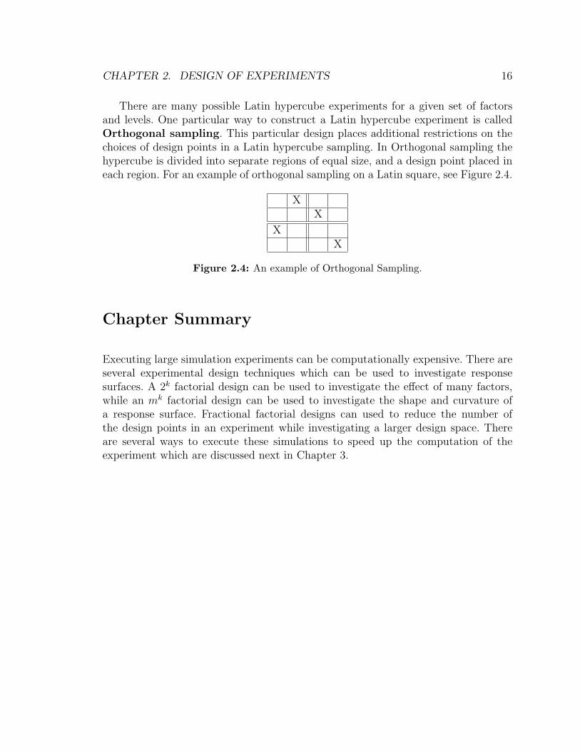
There are many possible Latin hypercube experiments for a given set of factorsand levels. One particular way to construct a Latin hypercube experiment is calledOrthogonal sampling. This particular design places additional restrictions on thechoices of design points in a Latin hypercube sampling. In Orthogonal sampling thehypercube is divided into separate regions of equal size, and a design point placed ineach region. For an example of orthogonal sampling on a Latin square, see Figure 2.4.
XX
XX
Figure 2.4: An example of Orthogonal Sampling.
Chapter Summary
Executing large simulation experiments can be computationally expensive. There areseveral experimental design techniques which can be used to investigate responsesurfaces. A 2k factorial design can be used to investigate the effect of many factors,while an mk factorial design can be used to investigate the shape and curvature ofa response surface. Fractional factorial designs can used to reduce the number ofthe design points in an experiment while investigating a larger design space. Thereare several ways to execute these simulations to speed up the computation of theexperiment which are discussed next in Chapter 3.

17
Chapter 3
Parallel Simulation Techniques
Simulation users often have access to computational resources such as servers, com-puter clusters, and other high performance workstations. These systems can havedifferent architectures; most often they have multiple processing cores, allowing themto run programs concurrently. This allows users to run tasks in parallel, and conse-quently there are many ways to harness the computational power of these systems.This chapter discusses how one might harness these computational resources to ac-celerate the execution of large scale simulation experiments.
3.1 Fine-Grained Parallelism
One approach to utilize all of the processors available is to distribute a single simula-tion across all of available processors. This is called fine-grained parallelism [27].In this case, different parts of the execution of the simulation must be separated torun on the individual processors.
There are many challenges associated with fine-grained parallelism. The developerof the simulator must be very careful during implementation to distribute the work inthe simulation to each of the processors evenly. In many simulations, this is especiallychallenging due to inherent data dependencies in the simulation execution, in whichone processor must wait on another processor’s result before it can proceed. There isalso overhead in communicating the result of some computation from one processor

CHAPTER 3. PARALLEL SIMULATION TECHNIQUES 18
to another.
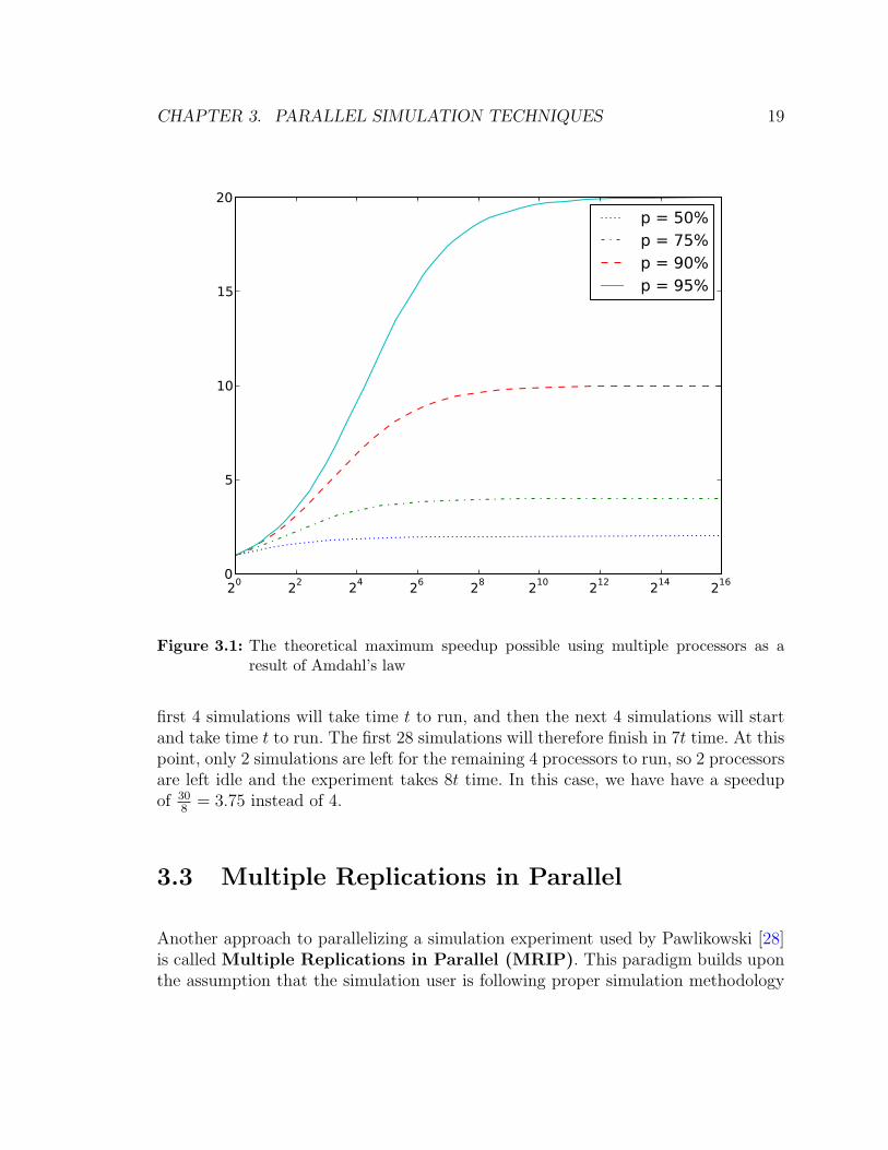
The performance of a fine-grained parallel simulation does not scale linearly withthe number of processors. The maximum theoretical speedup gained by parallelizinga process across n processors can be approximated by Amdahl’s law [21]. Let p bethe fraction of the process which can be parallelized and run on multiple processors,then Amdahl’s law states that the maximum speedup with n processors goes as
speedup =1
(1− p) + pn
The result of Amdahl’s law can be seen in Figure 3.1. For example, if p = 0.95, theneven using thousands of processors, there will only be a speedup of 20x. Fujimoto andNicol [18] discussed several techniques to increase the value of p such that simulationscan scale better with more processes.
3.2 Coarse-Grained Parallelism
An often simpler approach to balancing the work between many processors is calledcoarse-grained parallelism [27]. Coarse-grained parallelism distributes the workof the entire simulation experiment across many processors by assigning a single,sequential simulation to each processor. This allows processors to work independentlyof one another thereby eliminating overhead in synchronization and communication.
In coarse-grained parallelism, no processor ever needs to wait for the result of acomputation performed by another processor. Furthermore, the processes are inde-pendent, which eliminates all synchronization overhead. This is therefore an embar-rassingly parallel problem and thus p ≈ 1 and by Amdahl’s law:
speedup ≈ 1
(1− p) + pn
=11n
= n
This result is only applicable where the number of simulations which need to berun is a multiple of the number of processors available or greatly exceeds the numberof processors available.
For example, assume we have one design point with 30 simulations to run on 4processors, each of which takes time t to run. Using coarse-grained parallelism, the
CHAPTER 3. PARALLEL SIMULATION TECHNIQUES 19
20 22 24 26 28 210 212 214 2160
5
10
15
20p = 50%p = 75%p = 90%p = 95%
Figure 3.1: The theoretical maximum speedup possible using multiple processors as aresult of Amdahl’s law
first 4 simulations will take time t to run, and then the next 4 simulations will startand take time t to run. The first 28 simulations will therefore finish in 7t time. At thispoint, only 2 simulations are left for the remaining 4 processors to run, so 2 processorsare left idle and the experiment takes 8t time. In this case, we have have a speedupof 30
8= 3.75 instead of 4.
3.3 Multiple Replications in Parallel
Another approach to parallelizing a simulation experiment used by Pawlikowski [28]is called Multiple Replications in Parallel (MRIP). This paradigm builds uponthe assumption that the simulation user is following proper simulation methodology

CHAPTER 3. PARALLEL SIMULATION TECHNIQUES 20
and running multiple replications of each design point using different PRNG seeds.A central server dispatches independent simulation runs of the same design pointwith different seeds to be executed on different processors. During their execution,observations of performance metrics are reported to the central server overseeing theexecution of the simulations. This process can determine when enough observationshave been made to estimate performance metrics to within some tolerance specifiedby the user.
MRIP addresses the issue seen in coarse-grained parallelism when the number ofsimulations which need to be run are not significantly greater than the number ofavailable processors. Extending the example from Section 3.2, instead of running 30simulations on 4 processors, we instead run 4 simulations. Each of these simulationssimulates more virtual time, enough time to observe the minimum number of observa-tions required to estimate the metric to within the desired level of confidence. Thereis overhead both in running a separate server and communicating these observationsto the server. In comparison to coarse-grained parallelism however, the amount oftime spent in transient will be less, and all processors can be kept busy until theexperiment completes.
Chapter Summary
This chapter describes three techniques which can be used to speed up the compu-tation of a simulation experiment using multiple processors. Fine-grained simulationcan be used to parallelize a single simulation run, while coarse-grained simulationcan be used to run many independent simulations. The MRIP technique is a variantof coarse-grained simulation which can have better performance than coarse-grainedexecution. Next, Chapter 4 will describe how previous automation tools have inte-grated these experimental design and parallel simulation techniques to help users runexperiments efficiently.

21
Chapter 4
Previous Automation Tools
Several tools have been developed to automate one or more steps of the proper sim-ulation workflow for different simulators. In this chapter we introduce some of thesetools, namely CostGlue, ns2measure, ANSWER, Akaroa, SWAN-Tools, and JAMESII. The analysis of the features, strengths, and weaknesses of these tools helped usto reach key design decisions in the construction of the framework we present in thisthesis.
4.1 CostGlue
A software package called CostGlue was developed to aid telecommunication simu-lation users in storing and sharing their results. CostGlue provides an ApplicationProgramming Interface (API), in the programming language Python, which helpsone to store and access simulation results. CostGlue also has a modular architecturewhich allows for the development of plugins. These plugins can extend the originalfunctionality offered by CostGlue without becoming part of the project’s core sourcecode. [33]
The CostGlue API exposes all of the simulation results and meta-data to plugindevelopers. This allows for the development of plugins which can be used to conductstatistical analysis, generate figures, or export results into a format accessible by otherpost-processing tools such as R [6], SciPy [7], Octave [4], or Matlab [3]. The CostGlue

CHAPTER 4. PREVIOUS AUTOMATION TOOLS 22
developers also discuss the possibility of developing external processes which could beused to expose results stored in the CostGlue database via a publicly available webapplication. [33]
CostGlue, however, does not automate the process of parsing the results in theoutput from the simulation and therefore, does not prevent errors in this stage ofthe simulation workflow. Similarly, CostGlue does not provide facilities to process theresults from the simulation to extract the metrics of interest. This introduces anotherpotential area for errors to be made in the simulation workflow. Finally, users mustimport their results into CostGlue using custom developed scripts, which can againintroduce opportunities for errors to be made in the simulation workflow. All threeof these issues can lead to results which are not credible.
The CostGlue project demonstrates several desirable capabilities for handling sim-ulation data. Though the project is no longer under active development, these lessonscan be applied to future projects. The modular architecture for accessing simulationresults allows developers to easily extend the tool for their needs. Users can thenshare the tools they have developed to help other users in the simulation community.
4.2 ns2measure & ANSWER
While the CostGlue framework provides means for storing and accessing simulationresults it does not provide any facilities for collecting statistics from a simulator.Cicconetti et al. [15] has a project called ns2measure which addresses this issues andeases the process of extracting simulation metrics. Andreozzi et al. [12] also developeda tool called ANSWER which builds upon the functionality provided in ns2measureto help users automate large simulation experiments.
The ns2measure project aims to ease the process of collecting statistics duringsimulation execution using the network simulator ns-2. Ordinarily, when using ns-2,a trace of the network activity is written out to the file system for posterior analy-sis. Users must then carefully process these trace files to extract the statistics theyare interested in studying. Processing these results is often conducted with unveri-fied scripts which can produce biased or erroneous results. The ns2measure projectprovides a framework to collect statistics during the execution of the simulation it-self. Furthermore, it provides statistical analysis tools which help users conduct morestatistically sound simulation experiments. [15]

CHAPTER 4. PREVIOUS AUTOMATION TOOLS 23
A project called ANSWER, developed by the same research group at the Uni-versity of Pisa, Italy, works in harmony with ns2measure. While ns2measure aidsa user in gathering accurate statistics for a single design point, ANSWER helps toautomate running large scale simulation experiments with hundreds or thousands ofdesign points. This process is accelerated by distributing independent simulationsacross multiple available processors using coarse-grained parallelism. ANSWER alsoprovides web-based tools for interfacing with collected results.
These two software tools, ns2measure and ANSWER, offer many important fea-tures to simulation users. First, ns2measure provides mechanisms to extract observa-tions of performance metrics directly during simulation execution. When ns2measureis used in conjunction with ANSWER, simulation users can easily conduct a simple,credible simulation experiment using ns-2. One major shortcoming of ns2measure andANSWER is that they can only be used with ns-2.
4.3 Akaroa
In contrast to ANSWER, the Akaroa project developed by Pawlikowski [28] usedMRIP as described in Section 3.3 to accelerate running a single design point insteadof an entire experiment. The Akaroa project was originally developed for use withns-2, but it has since been ported to work with other simulators such as OPNET++.Pawlikowski [28] believes it can be adapted for use with other stochastic networksimulators as well.
While Akaroa demonstrates important functionality in software automation tools,it has a few shortcomings. Akaroa can only be used to execute a single design point.This requires users to manage each of the design points in their experiment manu-ally. Because users can make mistakes when managing the execution of these designpoints, we would like future tools to use MRIP to automate the entire experiment.Furthermore, Akaroa does not integrate with other tools such as ANSWER whichcan help users manage their simulation experiments. Finally, the Akaroa project re-quires permission from the authors to use for any application outside of teaching andnon-profit research activities.

CHAPTER 4. PREVIOUS AUTOMATION TOOLS 24
4.4 SWAN-Tools
One of the first software projects which attempted to automate running an entiresimulation experiment to ensure the credibility of results was the SWAN-Tools projectdeveloped at Bucknell University by Kenna [23], and Perrone et al. [31]. SWAN-Toolswas developed for use with the Simulator for Wireless Ad Hoc Networks (SWAN).The tool guides the user through all the steps of a proper simulation experiment, anddemonstrates many important functions in the automation of simulation experiments.
SWAN-Tools helps the user to create valid experiments and run independent sim-ulations in parallel across many physical computers. Also, the tool aids the user indata analysis by presenting results to be viewed in a web browser, to be downloadedand used with a statistics package, or to be graphically presented using proper plot-ting techniques via a web based interface. Lastly, the tool makes the results availablevia a website to which any scholarly article can be linked.
The lack of flexibility in this tool is its major shortcoming. It was built exclusivelyfor use with SWAN, and used a simulation model which was hard-coded into the tool.These constraints limit the potential uses for the tool. However, the aforementionedfeatures which guide the user through all steps of a proper simulation experiment canbe applied to future automation frameworks.
4.5 James II
The James II project takes a different approach to automating elements of propersimulation workflow. Instead of building tools which work in tandem with a specificsimulator, JAMES II provides a framework upon which simulators can be built. It hasa modular architecture with plugins for problem domains ranging from ComputationalBiology to Computer Networks. [22]
Once a simulation model has been defined using the JAMES II framework, thereare tools available to help run simulation experiments. Also, there are plugins whichhelp users use both coarse- and fine-grained parallel simulations. Furthermore, JAMESII provides facilities for storing and analyzing results.
The simulation must use the JAMES II core framework in order to take advan-

CHAPTER 4. PREVIOUS AUTOMATION TOOLS 25
tage of the several available plugins. Additionally, since the JAMES II framework isJava-based, all JAMES II simulators must be written in Java. While JAMES II hasan interesting architecture and feature set, many of the features for automating simu-lation experiments are not compatible with simulators which are not specifically builtfor this framework. The modular architecture of JAMES II, like CostGlue, allows itto be more widely applicable to different problem domains.
4.6 Lessons Learned
These tools have demonstrated several features and functions which are importantfor future automation tools to incorporate.
• A plugin system to allow users to customize the tool to their needs.
• A guiding user interface to help inexperienced users along.
• Parallel simulation techniques such as MRIP.
• A web interface to view the experiment configuration and results.
These ideas will be incorporated into my framework, SAFE, described next inPart II.
Chapter Summary
Several tools have been developed which automate different aspects of the propersimulation workflow. These tools demonstrate important functionality: output pro-cessing, output storage, distributed execution, rigorous statistical methods, and aguiding user interface. Lessons learned from these tools will be incorporated into myframework described next in Part II.

Part II
The Simulation AutomationFramework for Experiments
26

27
Chapter 5
Architecture
The Simulation Automation Framework for Experiments (SAFE) addressesmany of the aforementioned problems in both simulation usability and credibility.This chapter discusses SAFE’s architecture and feature set which has been designedto address the following general goals. The framework should:
• Be flexible and extensible.
• Automate the simulation workflow so as to ensure the credibility of the experi-mental process.
• Use the MRIP methodology to accelerate the execution of experiments.
• Include a web-based component to allow for the visualization of experimentalresults.
• Present differentiated interfaces which meet the needs of novice and experiencedsimulation users.
• The framework should be flexible such that it can be extended to work withother simulators. This is not to say that SAFE can be extended to work withevery possible simulator. Although existing simulators only available in binaryformat would be challenging to integrate with SAFE, it should be relativelystraightforward to modify open source simulators to work with the framework.
CHAPTER 5. ARCHITECTURE 28
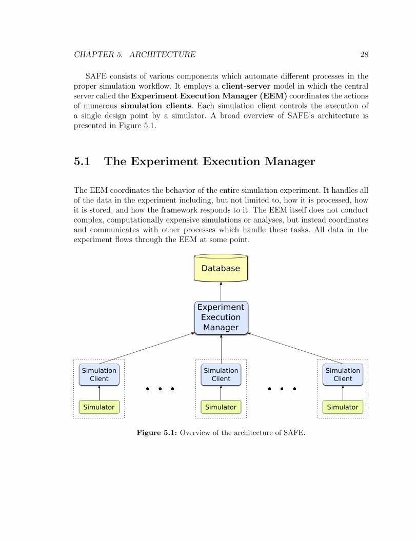
SAFE consists of various components which automate different processes in theproper simulation workflow. It employs a client-server model in which the centralserver called the Experiment Execution Manager (EEM) coordinates the actionsof numerous simulation clients. Each simulation client controls the execution ofa single design point by a simulator. A broad overview of SAFE’s architecture ispresented in Figure 5.1.
5.1 The Experiment Execution Manager
The EEM coordinates the behavior of the entire simulation experiment. It handles allof the data in the experiment including, but not limited to, how it is processed, howit is stored, and how the framework responds to it. The EEM itself does not conductcomplex, computationally expensive simulations or analyses, but instead coordinatesand communicates with other processes which handle these tasks. All data in theexperiment flows through the EEM at some point.
Database
ExperimentExecutionManager
SimulationClient
Simulator
SimulationClient
Simulator
SimulationClient
Simulator
Figure 5.1: Overview of the architecture of SAFE.

CHAPTER 5. ARCHITECTURE 29
The EEM accepts several input files which specify options in the EEM and definethe experiment to run. The languages which describe these inputs are described laterin Chapter 6. Using the information gathered from these input files, the EEM com-putes all of the design points in the experiment. The EEM then manages dispatchingthe necessary simulations to the available machines to be executed using an MRIPstyle parallelization technique. The Simulation Client, as described in more detail inSection 5.2, reports results back from the simulator to the EEM. The EEM must alsocoordinate how these results are handled after they are received from the simulationclient.
One of the EEM’s primary responsibilities is handling all interactions with thedatabase where SAFE stores all of its data. (The database itself will be discussed inChapter 8.) All results from the simulator are sent to the EEM which processes thedata and stores the results in the database. When the experiment is complete andusers need to conduct posterior analysis of their results, they must access their resultsthrough the EEM which helps to ensure that the results are accessed and processedproperly.
The EEM is also responsible for conducting proper statistical analyses. In SAFE,the transient and the end of the design point’s execution are both detected by externalprocesses. Within this design, the EEM is responsible for forwarding the intermediateresults to each of these processes in addition to the database. The EEM monitorsthese processes to know when the transient has passed and later when the designpoint should be terminated. This architecture can be seen in Figure 5.2.
SAFE has support for plugins, which extend its functionality, much like Cost-Glue and JAMES II. The plugins and any of their associated options are configuredthrough the experiment configuration language described in more detail in Section6.2. Currently, there are plugins for parsing the experiment description file, as well asgenerating all of the design points. There is also a hook to allow users to incorporateother plugins which manipulate data. The plugin system allows SAFE to be adaptedto current and future needs of the simulation user.
5.1.1 Asynchronous / Event-Driven Architecture
Two of the major requirements of the EEM are responsiveness and availability: theEEM must respond or react quickly to different actions and events so as to be readyfor the next event. By design, the tasks which the EEM executes are seldom ever

CHAPTER 5. ARCHITECTURE 30
Figure 5.2: Architecture of the interactions between the EEM and transient and run lengthdetection processes.

CHAPTER 5. ARCHITECTURE 31
computationally expensive or long-running, so that the EEM can react quickly to allinputs.
This type of application is often implemented using the reactor design pattern[34]. This design pattern yields an event-driven programming model in which theapplication waits for an event to happen, and a method known as a callback is calledto respond to the event and any associated data. After a callback is processed, thereactor drops back into the main loop where it waits for the next event to occur.There are many algorithms to decide when an event happens, but for networkedapplications such the EEM, the most common mechanism is to use the select()
system call, which returns when a file descriptor is ready to be read from or writtento.
An example of the benefits of this event-driven programming paradigm is queryinga database. In most synchronous programming models, when a query is made tothe database, the execution of the program blocks, or waits until the result of thequery is made accessible. This can simplify the programming model because one isassured that when the query returns, all of the results are available. In an applicationwhich strives to achieve high availability however, this programming model is ratherrestrictive, because the server is unresponsive while the program waits for the resultfrom the database. This time can be used to respond to other events, which otherwisewould have to wait until after the database has returned.
This behavior can be seen in Figure 5.3. Let the blue sections represent the timespent processing a database request, the orange is a response to a request for anotherdesign point, and the green is another database request. At some time as in Figure5.3, the request for the next design point is received. In the asynchronous case, theprocess is idle and can respond to the request immediately. In the synchronous case,the process is busy, and cannot begin to service the request until it has processedthe results from the database. Similarly, the database request in green is dispatchedbefore a request has been received for the blue database request. The reply from thegreen database request can be handled while the process waits for the result of thegreen database query. Consequently, the asynchronous programming model allows forthe process to handle different events in the system while it waits for other events tooccur.
The EEM is implemented in the programming language Python [5] and reliesheavily on the asynchronous, event-driven library called Twisted [8] which implementsthe reactor design pattern. Using this library, callbacks can be defined to handleresults from the simulation client, query results from the database, handle messages

CHAPTER 5. ARCHITECTURE 32
time
Async
Sync
Figure 5.3: A visual depiction of the benefit of an asynchronous vs. a synchronous pro-gramming model
from external processes used to detect transients, and many other types of events.
5.1.2 Dispatching Design Points
In coordinating the execution an experiment, the EEM dispatches to different comput-ers the simulations which correspond to various design points. We can estimate howthe distributed execution of the experiment affects the time to completion. In total,we will assume N samples must be generated for each design point such that metricscan be estimated to within the desired confidence level. When these N samples havebeen generated, the design point’s execution can be terminated. The simulation ofeach design point includes a number of independent replications, each of which must

CHAPTER 5. ARCHITECTURE 33
incur the cost of “warming up” to the end of its transient. We say that t samples arecollected during this period. The data deletion method requires that none of thesefirst t samples be used in estimating the desired metrics.
If we have r independent simulations replicating the same design point, whichcombined will generate the required N samples, on average, each replication needs togenerate N
rpost-transient samples. Then on average, each simulation will run until
is has generated t + Nr
samples. In total, across all r replications, the total numberof samples collected is then r(t + N
r) = rt + N . While the work to produce the N
samples is needed, the generation of the rt samples is only productive in the sensethat it allows replications to move beyond their transient.
To put this in perspective, consider the following example in which each simulationexecutes to 1000 s of simulated time, the transient is 100 s, and we have r = 30replications of the design point. We see that 30 × 1, 000 s = 30, 000 s of simulatedtime are executed, but only 30× (1, 000−100) s = 27, 000 s of simulated time producestatistically useful samples. This means 3, 000 s, or 10% of simulated time is used toproduce data which is disregarded in rigorous statistical analyses.
Although this analysis makes some simplifying, unrealistic assumptions, it demon-strates the overhead of simulating the transient. A better model would assume thetransient and run length are random variables. There exist several techniques to dis-patch simulations to utilize efficiently the computational resources in light of theoverhead of the transient.
One dispatching algorithm is to dispatch a single design point at a time to all pavailable processors. Each processor continues simulating the same design point untilthe EEM has determined that enough observations of the metrics of interest have beencollected. At this point, all of the remote hosts terminate the active simulation, andthe next design point can begin execution. This is how one would conduct a simulationexperiment using MRIP in the Akaroa 2 project [28]. Using this algorithm, we wouldsimulate approximately pt units of simulated time in transient.
In a simulation experiment we have many design points which can be processedconcurrently across our computational resources. Consequently, if each design pointis dispatched to at most n processors where n < p, there will be multiple designpoints running concurrently. Each design point will simulate approximately nt unitsof simulated time in transient in comparison to pt in the previous algorithm.
I developed a design point dispatching algorithm for SAFE which is a variant

CHAPTER 5. ARCHITECTURE 34
on these existing algorithms. In this algorithm, the design point which has seen thefewest results is dispatched first. This algorithm seeks to minimize the number ofindependent simulations which are executed for each design point (in essence, n foreach design point) so as to minimize the time spent in transient. This method can befurther adapted to set a minimum number of independent simulation runs n so as toreduce any bias from the choice of PRNG seed.
5.1.3 Web Manager
As a result of using an asynchronous programming model, the EEM can respond toa vast array of different types of events by installing new callbacks. This allows theEEM to expose data and parts of its state via a web-based interface, called the webmanager. Furthermore, because the EEM and the web manager are all contained ina single process, users can control aspects of the experiments execution from the webinterface.
As previously stated, one of the principal goals of SAFE is to provide a frameworkwhich both novice and experienced simulations users can employ to automate theirsimulation experiments. While more experienced users may gain more power throughusing command line oriented tools, a novice simulation user may feel more comfortableusing a web browser to control their experiment. The web manager allows for thisuse case by allowing a user to create an experiment by uploading the necessary inputfiles (described in more detail in Chapter 6), and using the web manager to start orstop the execution of the experiment.
Another use case for the web manager is to allow users to view their results via theweb. Again, this allows the novice simulation user to analyze results without requiringmore sophisticated scripts or command line oriented tools. More importantly, the webmanager exposes the complete experiment setup coupled with results. This allowsusers to publish their results to the web such that people around the world can viewthem, and link back to those results from any publication. These users can also repeatthe same experiment by downloading the input files for the specific experiment. Thistype of functionality was demonstrated by Perrone et al. [31] to significantly enhancethe credibility of published results by ensuring repeatability.
A feature to be incorporated in the web manager in the future is a plotting tool.Such a tool would guide the user through the generation of a plot. This type offunctionality is available in both SWAN-Tools [31], and ANSWER [12]. This not only

CHAPTER 5. ARCHITECTURE 35
provides an intuitive interface to the simulation user, but also to others interested inanalyzing the data after the results have been published. The web manager is a majorarea of future work under the continued funding of the NSF [20].
A common architecture for exposing data to clients on the web is called Rep-resentational State Transfer (REST); this model was first defined by Fielding[17] in his doctoral dissertation. REST defines how web applications can be queriedfor different resources. This allows developers to interact with web-based applicationsby querying for specific information. Furthermore, it allows for external applicationsto be developed which can access the information made accessible through this web-based API. This architecture is applied in the web manager which allows for externaldevelopers to interface with the web manager to query for results and control other as-pects of the behavior of the EEM through both the web browser as well as customizedscripts.
5.2 simulation client
The EEM is responsible for orchestrating how different processors contribute to theexecution of the experiment. It does so by communicating with a process called thesimulation client running on each computer (local or remote) participating in theexecution of the experiment. The simulation client manages how simulations are ex-ecuted, and how results are reported back to the EEM.
The first role of the simulation client is to connect to the EEM and register asan available host for the execution of simulations. In so doing, the simulation clienttransmits important details about its local environment such as the operating systemversion, architecture, etc. (e.g. GNU/Linux Kernel 2.6.33 Intel x86 64). If for anyreason problems are found which can be correlated with the collected data, thenhaving this information can be useful in detecting any problems, or disregarding anyresults.
The next step in the execution of the simulation client is to request a design pointto run. The EEM replies with a design point and any information required to startthe simulation running (e.g. the PRNG seed). The simulation client then spawns anew process for the simulator itself. While the simulator is processing, the simulationclient still has several responsibilities.

CHAPTER 5. ARCHITECTURE 36
The simulation client must continue to listen for instructions from the EEM. Atany point, the EEM can send a message informing the simulation client that theexperiment is complete and it should terminate the simulator and gracefully shutdown the process. The EEM can also inform the simulation client that the activedesign point is complete, in which case the simulation client should terminate theactive simulation, and then request the next design point to simulate.
The simulation client must also listen for results from the simulator itself. If thesimulator can output intermediate results during execution, the simulation client canforward these results to the EEM for storage and post-processing. If the simulatorcannot forward intermediate results, these results must be sent to the EEM upon thetermination of the simulation.
The simulation client, unlike the EEM, is not simulator specific. The simulationclient abstracts the details of the simulator away from the EEM allowing for the pos-sibility of using the EEM with different simulators. The simulation client decouplesthe EEM from the simulator itself allowing the EEM to be more general. Also, thefunctionality needed in a simulation client is largely the same between different sim-ulators, and therefore the development of a new simulation client for a new simulatorcan be streamlined by following the example of previous code.
The requirement of the simulation client to be listening and acting upon data froma few data sources lends itself to the reactor design pattern described in Section 5.1.1.Currently, my simulation client implementations are all implemented in Python usingthe Twisted Library just as the EEM is, but it is possible to develop a simulationclient in another language such as C or C++. In the development of the simulationclient, one must take care to avoid busy-waiting and using processors cycles to stalland wait for data from a data source. The simulation client should be as light aprocess as possible to leave the systems resources available to the simulator itself.
Current simulation client implementations are rather simplistic. A future devel-opment which would likely provide greater performance is to develop a simulationclient which is capable of managing many simultaneous simulators on a single host.This could provide slightly better performance for systems with a large number ofprocessors which could run a single simulation client instead of a simulation client foreach processor.

CHAPTER 5. ARCHITECTURE 37
Chapter Summary
The SAFE project uses a client-server programming model. By abstracting the im-plementation details associated with integrating SAFE with a specific simulator, theSAFE framework gains flexibility. This allows for the possibility of integrating SAFEwith other simulators. SAFE also defines a new way to dispatch design point to sim-ulation clients in such a way as to minimize the aggregate amount of time spentin transient. The EEM architecture allows for the integration of external tools andlibraries through other processes as well, such as through the use of the plugin sys-tem. Next, Chapter 6 describes the languages used to configure the experiment forexecution.

38
Chapter 6
Languages
SAFE’s architecture allows it to be flexible and adapt to a user’s many needs in theirsimulation experiments. It achieves this flexibility using a modular architecture, andexposes many options to users via configuration files. These configuration files arerequired to specify basic options for the EEM, plugins and plugin options, the designof the experiment, and the simulation model itself. These options are provided to theEEM as documents written according to configuration languages, which are definedby Andrew Hallagan in his Honors Thesis [19]. The languages are extensions fromXML (eXtensible Markup Language), which provides mechanisms for encoding infor-mation in formats that can be easily manipulated by computers. To fully understandthe benefits of using XML, it is necessary to first describe its structure.
6.1 XML Technologies
The XML language defines a text-based document format which is designed to besimple and easy to parse/interpret with a computer program. The World Wide WebConsortium which defined the XML language standard through a set of simple ruleswhich define how a valid XML document is formed and structured. [9] The simplenature of these rules allow XML to be widely applicable in many different problemdomains.

CHAPTER 6. LANGUAGES 39
An XML document is composed of three main types of content. The basic buildingblock of XML is called an element which encodes some piece of data, or even aconglomeration of data. An element is separated from other pieces of the documentusing opening and closing tags. A tag is a piece of text often called a tag-namesurrounded with “<” and “>” characters. A closing tag has the same tag name as theopening tag, but instead begins with “</”. An example of a valid XML element isseen in Listing 6.1.
<tagname>contents of the element</tagname>
Listing 6.1: An example XML Element.
The third type of content in an XML document is called an attribute. Attributescan be used to specify meta-data for an element. Attributes are specified inside ofthe tag surrounded by quotation marks. For example, we can add an attribute to thepreceding example as in Listing 6.2.
<tagname some_attr="attribute value">element contents</tagname>
Listing 6.2: An example XML Element with an attribute.
In an XML document, elements are often nested to encode the relationships be-tween the different pieces of data being encoded. Furthermore, the XML standardrequires there to be a single root element within which all elements are nested. Forexample, if we wanted to encode a probability distribution and its parameters, wecould nest the parameters in their own sub-elements as seen in Listing 6.3.
<factor distribution="Gaussian">
<mean>5.0</mean>
<variance>2.0</variance>
</factor>
Listing 6.3: An example of how elements can be nested in XML document.
The rules which define the XML language specification are very basic. They donot define the context or meaning of any of the tags or attributes in the documentsthemselves. This allows for the development of XML-based languages which furtherrestricts the XML language by specifying what types of tags can be used and how theycan be composed to form elements. In application, the specific tags and attributes aregiven context so that data can be easily encoded and transmitted between systems.

CHAPTER 6. LANGUAGES 40
For example, XML based languages are one of the primary means of encoding data onthe World Wide Web. The Hyper Text Markup Language (HTML) which is used toencode most of the web content viewed in web browsers is an XML-based language.The HTML specification defines a set of valid tags which web pages are encodedin. Modern web browsers understand the meaning of these tags and render the pageappropriately. For a brief example of HTML see Listing 6.4.
<html lang="en" xmlns="http://www.w3.org/1999/xhtml">
<head>
<title>A Sample Page Title</title>
</head>
<body>
<h1>The Heading on the Page</h1>
<p>A paragraph of text. <b>This sentence is all bold.</b></p>
</body>
</html>
Listing 6.4: An example HTML document.
These specifications for the newly created language can be defined in an XMLSchema. There exist languages for defining schemas including the Document TypeDefinition (DTD), XML Schema (XSD), and REgular LAnguage for XML Next Gen-eration (RELAX NG). Each of these languages has a different syntax.
Such a schema file can be used to validate a document. This functionality can actas a security measure to ensure that the document is well formed before a programtries to process its contents. In the context of simulation automation tools, inputscan be validated against the associated schema to ensure that the design point ormodel is valid. For example, a design point can be checked to ensure a level is givenfor each factor. Furthermore, it can check that all levels are valid (e.g. number ofwireless devices in the simulation is positive). Validation will enhance the credibilityof the final results by ensuring that all simulated models contain valid inputs to thesimulator.

CHAPTER 6. LANGUAGES 41
6.2 Experiment Configuration
The first language which SAFE uses to define an input file is the Experiment Config-uration Language. This language is used to define specific options and behaviors ofthe EEM for a specific simulator. This includes defining plugins and options specificto each of these plugins like CostGlue and JAMES II.
An important option in the execution of the simulation experiment is that everysimulator used to collect results in the experiment needs to be running the same ver-sion of the simulator. The experiment configuration language provides a mechanismto specify which version of the simulator the clients should be using. This versionis checked against the host specific information which each simulation client trans-mits to register as an available simulation client. This can be used to ensure that theversion matches that which is specified in the experiment configuration language.
There exist several different algorithms to detect the end of the transient. Whilethe technical details of these algorithms are outside the scope of this thesis, we expectusers will want to be able to apply these different algorithms to different experiments.The SAFE architecture allows developers to create their own transient detectionalgorithms in a separate script. SAFE then manages communicating all results tothese external processes. This process is managed through the plugin system, and theexperiment configuration language is used to specify options to the transient detectionalgorithm, and setup how the communication between the two processes is handled.An analogous plugin system exists to communicate with external processes whichestimate when a simulation experiment can be terminated.
Another application of plugins in SAFE is in results handling. SAFE defines de-fault behavior for how results are handled and stored, but additional plugins canbe implemented to allow for additional callbacks to be executed when results arereceived. This can be useful for users with more sophisticated usage patterns.
6.3 Experiment Description Language
The next language which we have developed for use with SAFE is the ExperimentDescription Language. This language encodes the experimental design and offers usersa flexible yet succinct language with which to define their experiment. The Experiment

CHAPTER 6. LANGUAGES 42
Description Language is also an XML-based language.
The Experiment Description Language is broken into two primary sections. Thefirst section encodes each factor, and all of the levels which it can be associated within the given experiment. This section alone defines a complete factorial experimentaldesign.
The second section defines constraints on the full factorial design. It provides manymechanisms with which full factorial experiments can be pruned. For example, designpoints can be individually excluded from the full factorial experimental design. Moreuseful though in application is the ability to tie specific levels for different factorstogether, such that any combination which does not include both (or all), of thelevels will not be included in the experiment.
Parameters to random distributions form an illustrative example of this feature ofthe Experiment Description Language. For example, if some process can be modeledwith either a Gaussian or an Exponential distribution, then the factors µ and σ2 mustbe coupled with the Gaussian distribution while the factor λ must be coupled withthe Exponential Distribution. If we use the factors and levels described in Table 6.1a,there are a total of 2×3×3×3 = 54 design points in the full factorial design. However,the vast majority of these design points are not valid based on the aforementionedconstraints regarding the parameters to each distribution. The six valid design pointscan be seen in Table 6.1b.
Factor Valid LevelsDistribution Gaussian, Exponential
µ N/A, 5, 10σ2 N/A, 0, 1λ N/A, 10, 20
(a) A list of factors and levels.
Distribution µ σ2 λGaussian 5 0 N/AGaussian 5 1 N/AGaussian 10 0 N/AGaussian 10 1 N/A
Exponential N/A N/A 10Exponential N/A N/A 20
(b) The set of valid design points.
Table 6.1: The full factorial design in Table (a) yields many design points with invalidparameter values. The set of valid design points is seen in Table (b).
The Experiment Description Language can be used to construct any experimentaldesign space. This allows users to customize their experiment specifically to investi-gate certain qualities or quantities in the system while reducing the number of designpoints which needs to be executed. It also allows for users to describe experimental

CHAPTER 6. LANGUAGES 43
designs such as fractional factorial designs and Latin hypercubes or any arbitraryexperimental design space.
6.4 Boolean Expression Objects
The Experiment Description Language is parsed by a SAFE plugin, thereby allowingothers in the simulation community to extend the language, and adapt the parserplugin for the new language. The parser plugin must communicate the factors andlevels as well as the restrictions to SAFE which in turn generates the design pointsthrough the design point generator plugin.
I have developed a standard data structure, which I have named the BooleanExpression Object, for encoding the constraints on the full factorial design. This datastructure encodes a boolean expression which can be applied to a design point todetermine if it is contained within the experiment. In the example in Table 6.1, wecan encode the boolean expression:
Distribution is Gaussian and µ is not “N/A”, and σ2 is not “N/A” and µis “N/A” or Distribution is Exponential and µ is “N/A”, and σ2 is “N/A”and µ is not “N/A.”
This expression is stored in a tree-like object which can be traversed to evaluatewhether a design point is contained in an experiment or not. Using the Boolean Ex-pression module which I have developed for SAFE, this expression would be encodedas in Listing 6.5.
The resulting expression object, can then evaluate a design point, dp withexpression.evaluate(dp). These boolean expression objects can be automaticallyconstructed during the parsing of the Experiment Description Language and thenapplied during design point generation to determine which design points in the fullfactorial design are included in the user’s experiment.
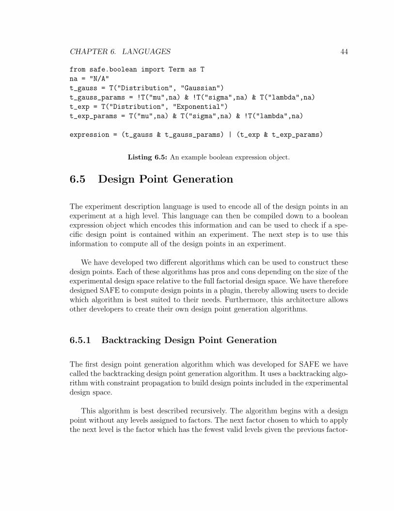
CHAPTER 6. LANGUAGES 44
from safe.boolean import Term as T
na = "N/A"
t_gauss = T("Distribution", "Gaussian")
t_gauss_params = !T("mu",na) & !T("sigma",na) & T("lambda",na)
t_exp = T("Distribution", "Exponential")
t_exp_params = T("mu",na) & T("sigma",na) & !T("lambda",na)
expression = (t_gauss & t_gauss_params) | (t_exp & t_exp_params)
Listing 6.5: An example boolean expression object.
6.5 Design Point Generation
The experiment description language is used to encode all of the design points in anexperiment at a high level. This language can then be compiled down to a booleanexpression object which encodes this information and can be used to check if a spe-cific design point is contained within an experiment. The next step is to use thisinformation to compute all of the design points in an experiment.
We have developed two different algorithms which can be used to construct thesedesign points. Each of these algorithms has pros and cons depending on the size of theexperimental design space relative to the full factorial design space. We have thereforedesigned SAFE to compute design points in a plugin, thereby allowing users to decidewhich algorithm is best suited to their needs. Furthermore, this architecture allowsother developers to create their own design point generation algorithms.
6.5.1 Backtracking Design Point Generation
The first design point generation algorithm which was developed for SAFE we havecalled the backtracking design point generation algorithm. It uses a backtracking algo-rithm with constraint propagation to build design points included in the experimentaldesign space.
This algorithm is best described recursively. The algorithm begins with a designpoint without any levels assigned to factors. The next factor chosen to which to applythe next level is the factor which has the fewest valid levels given the previous factor-

CHAPTER 6. LANGUAGES 45
level assignments. The algorithm picks one of these valid levels, applies it, and recursdown to the next most constrained factor. The set of valid levels for all remainingfactors is updated based on the boolean expression object. The algorithm recurs downuntil all factors have had levels assigned, at which point a valid design point has beenconstructed. From there, the algorithm backtracks and chooses other level choices soas to construct all of the valid design points in the experiment. Pseudocode for thisalgorithm is found in Listing 6.6.
Require: The backtrack function is called initially with:
• experiment← ∅.• remaining as all factors in the simulation model.
• current← ∅.• levels as a mapping from each factor to all associated levels.
function backtrack(experiment, remaining, current, levels)if remaining = ∅ then
add current to experimentreturn experiment
elsenextFactor ← most constrained factor in levelsfor level ∈ levels[nextFactor] do
current[nextFactor]← levelremove nextFactor from remainingnewlevels← updated levels for remaining factorsbacktrack(experiment, remaining, current, newlevels)add nextFactor to remainingcurrent[nextFactor]← null
end forend if
end function
Listing 6.6: Pseudocode for the backtracking design point generation algorithm.
The benefit of this design point generation algorithm is that it only explores designpoints which are included in the experimental design space. For experiments whichare a small subset of the full factorial design, this is particularly efficient. The price ofthis time efficiency is memory space. The recursive nature of the algorithm, whetherit is implemented recursively or iteratively using a stack, takes additional memory.The most memory is used in cases when the experiment is a large subset of the full

CHAPTER 6. LANGUAGES 46
factorial design.
6.5.2 Linear Design Point Generation
To address the weaknesses of the backtracking algorithm, we have developed an-other design point generation algorithm we call the Linear Design Point Generationalgorithm. Instead of only considering valid design points the linear design point gen-eration algorithm considers all design points in a full factorial design and evaluateswhether they are included in the actual experiment.
The linear design point generation algorithm iterates through all design points.(This can be done efficiently using the inverse of the design point id function describedlater in Section 8.3.) Each design point, design point, is evaluated using the booleanexpression object bool exp by calling bool exp.evaluate(design point).
When the experimental design space is a large subset of the full factorial design,there are relatively few design points considered which are not included in the experi-ment. In this case, there is little overhead associated with iterating through all of thepossible design points. If instead the experiment is only a small fraction of the fullfactorial design, then there is significant overhead iterating through the full factorialdesign space. Another advantage of the linear design point generation algorithm isthat it requires constant space.
experiment← ∅for designPoint in factorialDesign do
if designPoint is valid thenadd designPoint to experiment
end ifend forreturn experiment
Listing 6.7: Pseudocode for the linear design point generation algorithm.
6.5.3 Design Point Construction
These two design point generation algorithms compute a set of design points encodedas Python dictionaries where the factor is the key and the level is the value. Each of

CHAPTER 6. LANGUAGES 47
these dictionaries representing a design point must be encoded into a simulation modelwhich can be passed to the simulation client for execution. SAFE uses templates toaccomplish this task.
A template provides the structure of the simulation model, leaving placeholdersfor specific factor’s levels to be inserted into the model. The most simple simulationtemplate only requires a direct string substitution to construct the model. Somemodels require more structure, and structure which is dependent upon the levels inthe design point. This requires a more powerful template system. For this purpose,SAFE uses the template engine Cheetah which is based in Python. An example ofa Cheetah template can be found in Appendix C. Cheetah allows for conditionalstatements to be inserted into the template which can be executed to construct partsof the simulation model. Furthermore, Cheetah can execute loops to generate partsof models. Cheetah can, in fact, generate any text-based format and can thereforegenerate any simulation model. [2]
Once the simulation model has been generated using the template engine, thedesign point can be saved to the database. This allows results which are collected bysimulation clients to be linked to the appropriate design points. The design point isthen ready to be dispatched to the next available simulation client.
To speed up the startup time of the EEM, SAFE generates design points one ata time, as needed, when requests are made for the next design point from simulationclients. Design points are then generated one at a time, as needed. The design pointgenerator class is itself an iterator, and as such, the next design point can be generatedwith a simple call to next(). By constructing the next design point on an as neededbasis, SAFE is able to accelerate the startup process, and accept incoming simulationclient connections for faster computation. This architecture can reduce the overalltime a simulation experiment takes to execute.
Chapter Summary
Libraries and utilities for validating, generating and parsing XML based languagesare ubiquitous across most modern programming languages. Languages based in XMLcan be developed to describe input and output data necessary to conduct simulationexperiments. By building these language in XML, common tools can be adapted forour uses, and different components of a larger project can easily be written in different

CHAPTER 6. LANGUAGES 48
languages, or be executed in different environments sharing only the specification forthe XML based language. We have developed languages based in XML which areused to encode the experiment and its configuration to the EEM. These languagescan then be parsed to generate all of the design points in the experiment. Next,Chapter 7 describes how these design points can be communicated to simulationclients running on remote hosts.

49
Chapter 7
Inter-Process Communication
The architecture of SAFE defines many separate processes, many of which can runon remote computers. While this architecture allows for many features and greaterflexibility, it requires careful attention to how these separate processes communicate.In SAFE there are many types of inter-process communication (IPC) mecha-nisms which are used for different applications. A broad overview of the types of IPCmechanisms used in SAFE can be seen in Figure 7.1
The SAFE project provides MRIP functionality which requires communicationbetween simulations on networked machines and the central server. In SAFE, thecommunication between the simulator itself and the EEM is broken into two sepa-rate steps. The first step is to communicate results from the simulator itself to thesimulation client, and the second is to communicate the results from the simulationclient to the EEM.
7.1 IPC Mechanisms
The SAFE project is designed to be run on a UNIX platform. On such platforms thereare several different mechanisms available to communicate data from one process toanother. Each of these mechanisms has advantages and disadvantages for differentapplications. In this section I provide a brief description of pipes and socket basedIPC mechanisms which are employed in SAFE as seen in Figure 7.1. There exist

CHAPTER 7. INTER-PROCESS COMMUNICATION 50
ExperimentExecutionManager
Pipes
Pipes
Pipes
Pipes
Pipes
Pipes
TCPSockets
TCPSockets
Design Point
SimulationClient
Simulator
host
SimulationClient
Simulator
host
Pipe Pipe
Design Point
SimulationClient
Simulator
host
SimulationClient
Simulator
host
Pipe Pipe
SQL
Host
Database
Figure 7.1: Architecture of the framework with respect to inter-process communication.

CHAPTER 7. INTER-PROCESS COMMUNICATION 51
other IPC mechanisms such as fifos, UNIX sockets, shared memory, but thesemechanisms are not used in SAFE.
7.1.1 Pipes
One of the most simple forms of IPC available on UNIX based systems is called apipe. Pipes are implemented in the operating system itself, and therefore can onlybe used for communication between processes on the same physical machine. Theoperating system is able to synchronize the reading and writing from the pipe’s bufferto ensure the consistency of the data. Pipes are also unidirectional, but two pipes, onefor reading and one for writing, allow for bidirectional communication. Pipes exposedata to the receiving process as a stream. [35]
Pipes are created by a single process which then calls fork() to spawn a childprocess. The child process shares the open file table, and the thus file descriptorof the pipe to the parent process is available. The parent and child processes can thencommunicate on this pipe using the standard system calls read() and write().
7.1.2 Network Sockets
Pipes are a useful IPC mechanism, but they are restrictive in that they can only beused between related processes on the same host. Computer networks have been builtto facilitate the passing of information from one computer to another. There are manylayers of complexity in the network stack, which handle sending the electrical signaland routing the messages to the appropriate network node, but these technologies lieoutside of the scope of this thesis. These lower layers in the network stack allow for theabstraction in the transport layer of end-to-end communication between nodeson the network via what are called network sockets. [32]
Application developers can interact with these network sockets to communicatewith other processes on other computers. Two common transport protocols are usedwith sockets: the User Datagram Protocol (UDP), and the Transmission Con-trol Protocol (TCP). Since each of these protocols offers a different kind of com-munication model, the specific needs of applications dictate which one is preferable.
UDP is a minimalist protocol in which data is encapsulated in discrete packets

CHAPTER 7. INTER-PROCESS COMMUNICATION 52
or datagrams. A UDP packet carries a few pieces of metadata in its header, includingthe identification of source and destination ports to allow the multiplexing of packetflows to different applications. The UDP protocol is connectionless because it doesnot rely on the creation of a virtual circuit between sender and receiver before pack-ets begin to flow. Additionally, UDP promises only a best-effort in packet delivery,without hard guarantees of reliability. Finally, UDP is not order-preserving, thatis, packets can arrive at the destination in order different from that in which theywere sent. [32, 37]
On the other hand, TCP implements a channel which is both reliable and orderpreserving. Even though TCP requires the creation of a virtual circuit from sender toreceiver, it provides the abstraction of a continuous stream of bytes, delivered reliablyand in-order [32, 37]. To provide this communication model, TCP incurs significantoverhead and therefore it is not always the best protocol for every application. Time-sensitive applications, such as streaming audio or video, can tolerate packet loss muchbetter than it can tolerate higher end-to-end delays between sender and receiver; forthose applications UDP is a better choice. On the other hand, there exists anotherclass of applications which benefit from the communication model of TCP, which isstraightforward to use.
7.2 EEM ↔ Simulation Client
The first IPC mechanism used in SAFE allows for the EEM to communicate with eachindividual simulation client. To allow simulations to be distributed on local or remotehosts connected by a network, a network based IPC mechanism must be employed.This requires that the IPC mechanism chosen for this application be a network basedIPC mechanism. For this reason, a socket based IPC mechanism has been chosen forthe communication between the EEM and the simulation client.
Several types of messages must be exchanged by the EEM and the simulationclient; most of these are simulation results being reported. These are small messageswhich contain an individual result, a double precision floating point number, and afew pieces of metadata describing the result. These results reflect the execution of asimulation run and they must be captured and stored for posterior analysis. So thatnone of the results would go unrecorded due to packet loss between the simulationclient and the EEM, we elected to use TCP to interconnect the two processes.

CHAPTER 7. INTER-PROCESS COMMUNICATION 53
The communication between the EEM and the simulation client follows a protocolwith message types described as follows. Figure 7.2 illustrates how these message typesare used in the course of a simulation experiment.
• Register Message: Sent by the simulation client to the EEM when it firstconnects. It provides information about the local simulation environment.
• Next Simulation Request: Sent by the simulation client to the EEM after thesimulation of a design point terminates, or immediately following a Register
message. Represents the simulation clients asking the EEM for a new designpoint to run.
• Next Request Reply: Sent by the EEM to the simulation client as response toa Next Simulation Request message. Carries an XML document describingthe simulation model for a design point. The simulation client uses the XMLdocument to setup the simulation run, which is then executed.
• Result: Sent by the simulation client to the EEM upon receipt of a resultfrom the simulator. This message carries a sample of a metric generated bythe simulator, which is used by detectors for transient and run-length and alsostored in the database along with all data pertaining to the same experiment.
• Finished: Sent by the EEM to every simulation client which has been selectedto collaborate in the simulation of a given design point. This message indicatesthat, for this design point, enough samples of the results have been collected sothat the desired metric can be estimated within the user-specified confidence in-terval. Upon receiving this message, the simulation client terminates the currentrun and issues a Next Simulation Request.
• Terminate: Sent by the EEM to all simulation clients when all design pointsfor the experiment have been completed. Upon receiving this message, the sim-ulation client processes themselves terminate.
7.3 Simulator ↔ Simulation Client
The simulation client uses the information communicated from the EEM in the afore-mentioned protocol to control the initialization and communication with the simulator

CHAPTER 7. INTER-PROCESS COMMUNICATION 54
SimulationClientEEM
Register Message
Next Simulation Request
Next Simulation Reply (design point)
Result
Simulationof design point
Next Simulation Request
Next Simulation Reply (design point)
Simulationof design point
Finished
ResultResult
...
Result
Result
...
Next Simulation Request
...
Terminate Simulation Client terminates
Figure 7.2: Communication protocol used by EEM and simulation client.

CHAPTER 7. INTER-PROCESS COMMUNICATION 55
itself. The simulator and the simulation client are necessarily both run on the samemachine. This eliminates the need to use a network based communication mecha-nism, but it does not rule out network based IPC mechanisms as a viable solution forthis communication channel. There are two primary applications for communicationbetween these two processes: communicating intermediate results from the simula-tor to the simulation client, and informing the simulator to terminate gracefully atthe instruction of the EEM. For these two applications, I have chosen different IPCmechanisms.
To decide which IPC mechanism to use to pass results, I conducted several infor-mal tests. I found pipes to be an order of magnitude faster than socket-based IPCmechanisms. The simulation client spawns a child process for the simulation itself, sopipes can be used for this form of communication. For the simulation clients I havedeveloped, I have implemented the IPC between the simulation client and simulatoritself using pipes. While this is a fast and easy form of IPC, simulation clients forother simulators could choose to use alternative IPC mechanisms. The simulationspecific details of this design are described in more detail in Chapter 9.
Most simulators are not designed to be actively listening for data coming fromexternal processes through pipes or other file descriptors. Consequently, it could bechallenging to integrate the communication from the simulation client to the sim-ulation itself using pipes. The only type of information which the simulation clientneeds to send to the simulator is a message to gracefully terminate the simulation. Analternative to using pipes to communicate this one simple message is to instead use asignal. The simulator executes the signal handler when the simulation client sendsthe specific signal. This method terminates the execution of the simulation gracefully.
Using a combination of pipes and signals, SAFE can interoperate with many dif-ferent simulators, particularly those which are open source and can be easily modifiedfor use with SAFE. For simulators in which the source code cannot be easily modified,the simulation client must be developed to interact with the simulation to extract therelevant information. In the worst case scenario, the simulation client cannot commu-nicate directly with the simulator during its execution. In this case, the simulator canwrite results to the file system and the simulation client can parse all of the results toextract individual results to send to the EEM. This eliminates many of the benefitsof the MRIP architecture, but still allows the simulator to integrate with SAFE touse all of its additional automation features.

CHAPTER 7. INTER-PROCESS COMMUNICATION 56
7.4 EEM ↔ Transient and Run Length Detector
One of the plugins provided by SAFE allows for the computation of the transientdetection and the run length detection to be offloaded to an external process. Byoffloading this computation to a separate process, a few things are gained. First,the EEM is made more responsive because it spends less time blocking on statisticalcalculations. Second, it allows SAFE to integrate with other external tools and utilitieswhich can be used to estimate the transient and the run-length.
Much like the communication between the simulation client and the simulator,the communication between the EEM and the transient and run length detectionprocesses can be restricted to the local machine. Furthermore, the EEM is responsiblefor spawning the detection processes, and therefore pipes are a natural IPC mechanismto use to communicate results to these processes. Additionally, they are a fast IPCmechanism.
The plugin which is responsible for interacting with the detection algorithm couldhowever choose to use a different IPC mechanism. For example, one could implementa socket based solution and offload the computation of the transient and the runlength to a remote host. This type of solution could be explored further by users whoexperience high EEM latency or find the process to be unresponsive running on asingle machine.
Chapter Summary
There are several types of IPC which can be used to coordinate and communicate be-tween many components of SAFE. This chapter explores three main IPC mechanisms:pipes, TCP sockets and UDP sockets. It is determined that a TCP based protocol isthe best solution to communicate between the EEM and the simulation client. Pipesare then used to communicate both between the simulation client and the simulator,as well as between the EEM and transient and run length detection processes. Thesecollected results which are communicated between the simulator, simulation client,and the EEM are eventually stored as described next Chapter 8.

57
Chapter 8
Storing and Accessing Results
Chapters 5, 6 and 7 focused on the architecture of SAFE which allows for the designand configuration of a simulation experiment, and later how the experiment is actuallyexecuted across all of the components of the SAFE framework. This architecture existsto collect data which can be stored and accessed for further analysis. This chapterfocuses on the design considerations associated with storing and accessing the typeand quantity of data collected during a large simulation experiment.
8.1 Databases
SAFE employs a Relational Database System (RDBS) to store and access allof the simulation data, as well as any associated meta-data. Before explaining howSAFE interacts with the database itself, it is best to provide a brief introduction torelational databases.
8.1.1 Theory
A relational database is composed of a set of relations where a relation is defined asa set of tuples over a fixed set of attributes. Each tuple represents a real-world objectthat is described through a unique assignment of values on the attributes. Each rela-
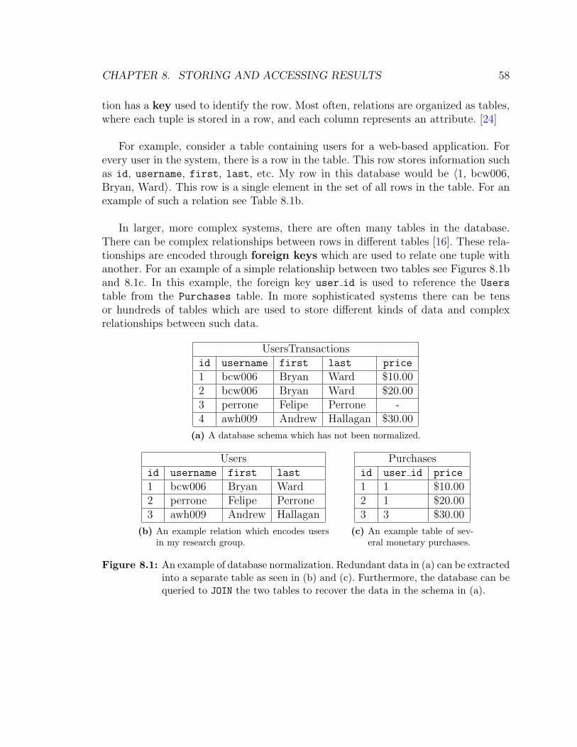
CHAPTER 8. STORING AND ACCESSING RESULTS 58
tion has a key used to identify the row. Most often, relations are organized as tables,where each tuple is stored in a row, and each column represents an attribute. [24]
For example, consider a table containing users for a web-based application. Forevery user in the system, there is a row in the table. This row stores information suchas id, username, first, last, etc. My row in this database would be 〈1, bcw006,Bryan, Ward〉. This row is a single element in the set of all rows in the table. For anexample of such a relation see Table 8.1b.
In larger, more complex systems, there are often many tables in the database.There can be complex relationships between rows in different tables [16]. These rela-tionships are encoded through foreign keys which are used to relate one tuple withanother. For an example of a simple relationship between two tables see Figures 8.1band 8.1c. In this example, the foreign key user id is used to reference the Users
table from the Purchases table. In more sophisticated systems there can be tensor hundreds of tables which are used to store different kinds of data and complexrelationships between such data.
UsersTransactionsid username first last price
1 bcw006 Bryan Ward $10.002 bcw006 Bryan Ward $20.003 perrone Felipe Perrone -4 awh009 Andrew Hallagan $30.00
(a) A database schema which has not been normalized.
Usersid username first last
1 bcw006 Bryan Ward2 perrone Felipe Perrone3 awh009 Andrew Hallagan
(b) An example relation which encodes usersin my research group.
Purchasesid user id price
1 1 $10.002 1 $20.003 3 $30.00
(c) An example table of sev-eral monetary purchases.
Figure 8.1: An example of database normalization. Redundant data in (a) can be extractedinto a separate table as seen in (b) and (c). Furthermore, the database can bequeried to JOIN the two tables to recover the data in the schema in (a).
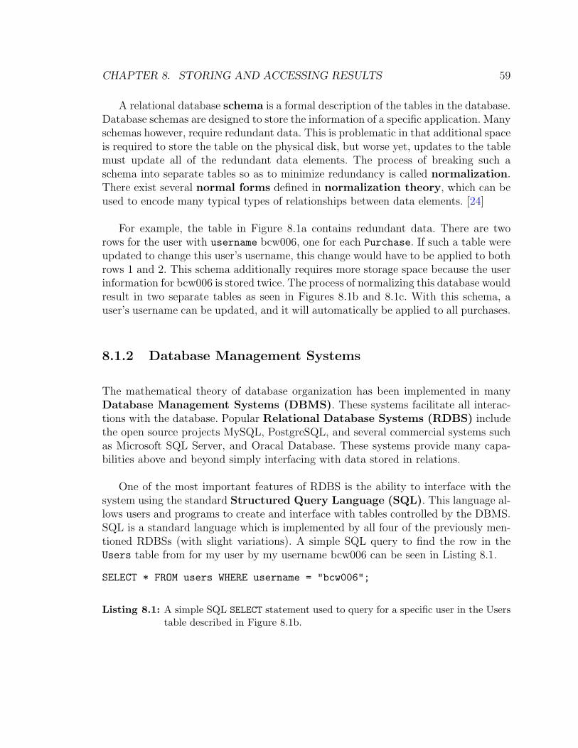
CHAPTER 8. STORING AND ACCESSING RESULTS 59
A relational database schema is a formal description of the tables in the database.Database schemas are designed to store the information of a specific application. Manyschemas however, require redundant data. This is problematic in that additional spaceis required to store the table on the physical disk, but worse yet, updates to the tablemust update all of the redundant data elements. The process of breaking such aschema into separate tables so as to minimize redundancy is called normalization.There exist several normal forms defined in normalization theory, which can beused to encode many typical types of relationships between data elements. [24]
For example, the table in Figure 8.1a contains redundant data. There are tworows for the user with username bcw006, one for each Purchase. If such a table wereupdated to change this user’s username, this change would have to be applied to bothrows 1 and 2. This schema additionally requires more storage space because the userinformation for bcw006 is stored twice. The process of normalizing this database wouldresult in two separate tables as seen in Figures 8.1b and 8.1c. With this schema, auser’s username can be updated, and it will automatically be applied to all purchases.
8.1.2 Database Management Systems
The mathematical theory of database organization has been implemented in manyDatabase Management Systems (DBMS). These systems facilitate all interac-tions with the database. Popular Relational Database Systems (RDBS) includethe open source projects MySQL, PostgreSQL, and several commercial systems suchas Microsoft SQL Server, and Oracal Database. These systems provide many capa-bilities above and beyond simply interfacing with data stored in relations.
One of the most important features of RDBS is the ability to interface with thesystem using the standard Structured Query Language (SQL). This language al-lows users and programs to create and interface with tables controlled by the DBMS.SQL is a standard language which is implemented by all four of the previously men-tioned RDBSs (with slight variations). A simple SQL query to find the row in theUsers table from for my user by my username bcw006 can be seen in Listing 8.1.
SELECT * FROM users WHERE username = "bcw006";
Listing 8.1: A simple SQL SELECT statement used to query for a specific user in the Userstable described in Figure 8.1b.
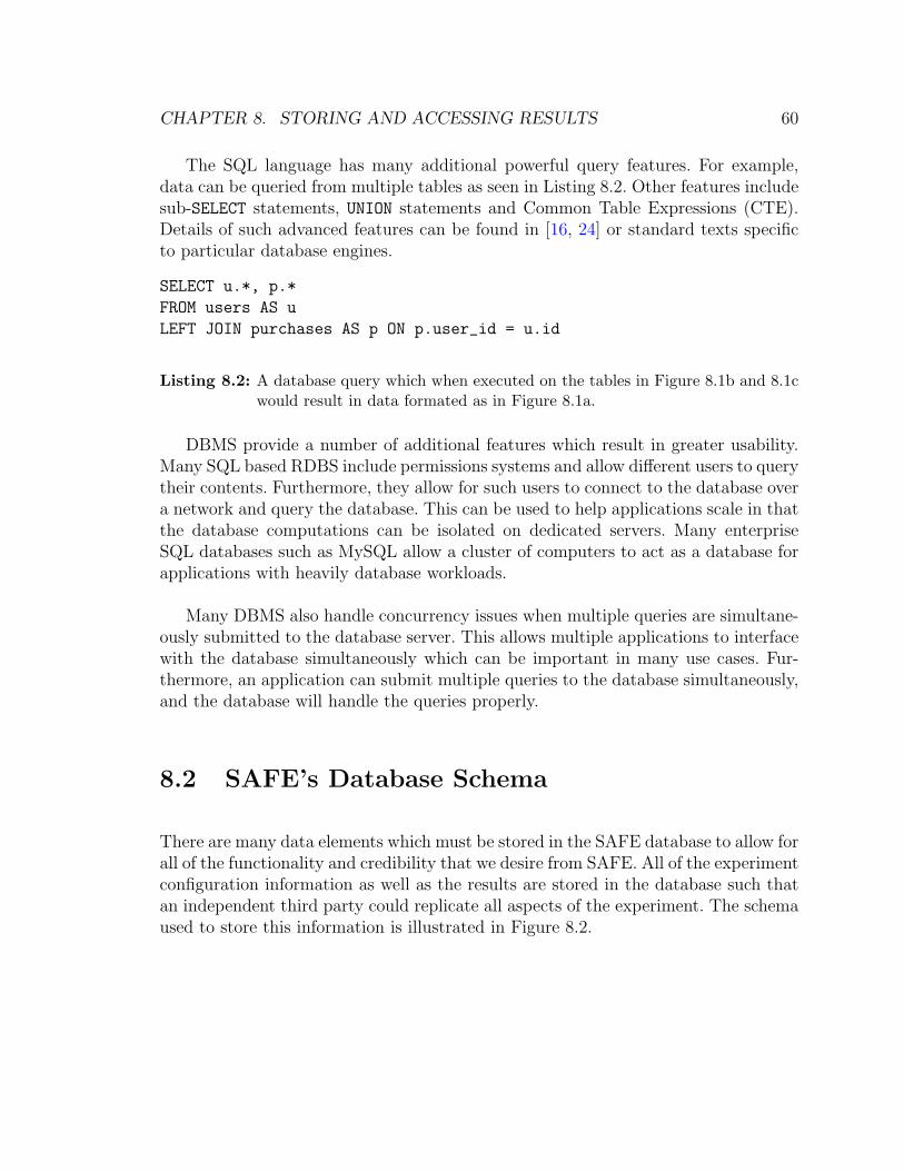
CHAPTER 8. STORING AND ACCESSING RESULTS 60
The SQL language has many additional powerful query features. For example,data can be queried from multiple tables as seen in Listing 8.2. Other features includesub-SELECT statements, UNION statements and Common Table Expressions (CTE).Details of such advanced features can be found in [16, 24] or standard texts specificto particular database engines.
SELECT u.*, p.*
FROM users AS u
LEFT JOIN purchases AS p ON p.user_id = u.id
Listing 8.2: A database query which when executed on the tables in Figure 8.1b and 8.1cwould result in data formated as in Figure 8.1a.
DBMS provide a number of additional features which result in greater usability.Many SQL based RDBS include permissions systems and allow different users to querytheir contents. Furthermore, they allow for such users to connect to the database overa network and query the database. This can be used to help applications scale in thatthe database computations can be isolated on dedicated servers. Many enterpriseSQL databases such as MySQL allow a cluster of computers to act as a database forapplications with heavily database workloads.
Many DBMS also handle concurrency issues when multiple queries are simultane-ously submitted to the database server. This allows multiple applications to interfacewith the database simultaneously which can be important in many use cases. Fur-thermore, an application can submit multiple queries to the database simultaneously,and the database will handle the queries properly.
8.2 SAFE’s Database Schema
There are many data elements which must be stored in the SAFE database to allow forall of the functionality and credibility that we desire from SAFE. All of the experimentconfiguration information as well as the results are stored in the database such thatan independent third party could replicate all aspects of the experiment. The schemaused to store this information is illustrated in Figure 8.2.

CHAPTER 8. STORING AND ACCESSING RESULTS 61
Experimentsid
name
configurations_id
template_id
descriptions_id
Configurationsid
configuration
Descriptionsid
descriptions
Templatesid
template
DesignPointsid
experiment_id
design_point_identifier
simulation_xmlResults
id
simulation_id
timestamp
object
metric
value
Simulationsid
design_point_id
host_id
Hostsid
ip
kernel
FactorsLevelsid
design_point_id
factor
level
Figure 8.2: SAFE database schema.
The contents of the tables shown in this schema are as follows:
• Configurations: This table stores the experiment configuration files.
• Descriptions: This table stores the contents of experiment description lan-guages.
• Templates: This table stores the contents of the templates used to generatethe simulation model.
• Hosts: The hosts table is populated when a new simulation client registers asan available simulation host. This table stores information about each host’slocal environment.
• Experiments: This table contains information about specific experiments. Ithas foreign keys to Configurations, Descriptions, and Templates such thatthese files can be used for multiple experiments without data duplication.
• DesignPoints: An experiment is by definition composed of a set of designpoints. This table contains all of the design points, a unique design point id
for each experiment described later in 8.3, and the XML model for the designpoint.
• FactorsLevels: A design point can have many factors, each with of which mustbe associated with a level. The FactorsLevels table stores these assignments.

CHAPTER 8. STORING AND ACCESSING RESULTS 62
• Simulations: For each design point in the experiment, many simulations areexecuted. This association is modeled with a foreign key to the DesignPoints
table. Because each of these simulations are run on a single host, the Simulationstable has a foreign key to the hosts table to model this association.
• Results: Each observation of a metric is stored in the Results table as asingle row. For each result, we record the simulated timestamp of the result, thesimulated object for which the result was gathered (e.g. which network nodereceived a packet), the metric, and the value of that metric. Each result is thenassociated with the Simulation it was gathered from using the simulation id
foreign key.
The most important result of this database schema is its ability to store and accessdifferent types of simulation models. The SWAN-Tools project described in Section4.4 hard-coded a single simulation model into both the database schema and the userinterface. By normalizing the database schema and separating the factors and levelsfrom the design points table, SAFE can be used with many simulation models.
8.3 Querying For Results
While the aforementioned database schema provides great flexibility in storing dif-ferent types of models, it can also make querying for specific design points and theirassociated results challenging. The primary challenge is that for each factor for whicha specific level is chosen, the FactorsLevels table must be JOINed. An example ofsuch a query can be found in Listing 8.3. Each JOIN requires O(n) time, and theproduct of all of these O(nj) JOINs where n is the number of rows and j is the to-tal number of joins. Thus this query can be slow when there are many factors andlevels which are specified. Unfortunately, this is a common use case when analyzingsimulation results.
One solution to this problem which was temporarily considered was to search theXML of the simulation model stored in DesignPoints table for specific factor’s levelvalues. While this approach does not require the query to JOIN the FactorsLevels
table n times, it requires a full text search of every design point’s XML in the ex-periment. Furthermore, the database engine cannot apply indices to accelerate suchqueries.

CHAPTER 8. STORING AND ACCESSING RESULTS 63
SELECT dp.*, r.*
FROM DesignPoints AS dp
LEFT JOIN Simulations AS s ON (s.design_point_id = dp.id)
LEFT JOIN Results AS r ON (s.id = r.simulation_id)
LEFT JOIN FactorsLevels AS f1 ON (dp.id = f1.design_point_id)
LEFT JOIN FactorsLevels AS f2 ON (dp.id = f2.design_point_id)
...
LEFT JOIN FactorsLevels AS fn ON (dp.id = fn.design_point_id)
WHERE dp.experiment_id = 1234 /* Some arbitrary experiment’s id */
AND f1.factor = "param_1" /* Some arbitrary factor to filter by*/
AND f2.level = "123" /* Some arbitrary level value */
AND f2.factor = "param_2" /* Another arbitary factor */
AND f2.level = "456" /* Another arbitary level */
...
AND fn.factor = "param_n"
AND f2.level = "789";
Listing 8.3: An example of a query which returns results for a design point based on nlevels.
The solution which I have developed for querying for results builds upon many ofthe ideas presented in the Design Point Generation Section, Section 6.5. The samealgorithms used to prune the full factorial design to generate the appropriate designpoints can be applied to prune the full factorial design to find the specific designpoints to investigate further. These same algorithms can therefore return a set ofdesign points for which to query the database for explicitly. One consequence of thisapproach is that more computation is required of the EEM. The computation of thespecific design points in the result set therefore cannot be conducted by the databaseengine.
For this approach to be efficient, a mechanism is required to query for a specificdesign point. There is a unique id associated with each row in the database, but thesevalues are determined by the database engine. The DesignPoints table therefore hasanother column which encodes a unique integer, the design point id, within theexperiment which can be calculated based on the factors and levels in a specificdesign point. This integer can be computed for each design point in the set of designpoints for which to query. An efficient database query can then be easily constructedwhich returns the proper design points.

CHAPTER 8. STORING AND ACCESSING RESULTS 64
To describe further how the design point id is computed, it is necessary toestablish a solid mathematical framework within which to work. Let F1, . . . , Fn befactors of the model. Each of these factors has a set of levels denoted L1, . . . , Ln.Then the set of design points simulated, D, is a subset of the cross product of thelevels, D ⊆ LF1 × . . .× LFn . Notationally, let d ∈ D be a design point, and di be thelevel associated with factor i in the design point. The design point id is then theproduct of an injective function f : LF1 × . . .× LFn → N.
To construct this function, first we define the bijective function gi : LFi→ N<|LFi
|which maps a level to the index of the level in the sorted list of levels. This functionis then used in the definition of f :
f(d) =n∑
i=1
(g(di)
n∏k=1
|Lk|)
As it turns out, this function is bijective. The inverse of this function can be appliedin the design point generation algorithm described in Section 6.5.2 to iterate throughall design points easily.
This function is best understood through an example. In a 24 factorial design thereare 16 design points. The function f assigns an ordering to these design points. Avisual representation of how f orders design points can be seen in Figure 8.3. In thisfigure, each cell represents a design point with a unique level assignment for each ofFactor 1 and Factor 2.
When the design points are generated and stored in the database, this function iscomputed and also stored. The database is setup with an index on this column, andthe constraint that the unique id for the table and this design point id in tandemare unique. This allows for quick lookups. When querying for results, the design pointsof interest can be computed from L1, . . . , Ln, and then f can be applied to each tupled. The database engine can then easily search for each of these design points.
Factor 1
Fac
tor
2 1 2 3 45 6 7 89 10 11 1213 14 15 16
Figure 8.3: A visual explanation of how the function f maps design points down to N.

CHAPTER 8. STORING AND ACCESSING RESULTS 65
Chapter Summary
This chapter briefly provides a background of relational databases, and demonstrateshow they can be used. These relational databases offer many capabilities which makethem very useful for storing simulation results. For these reasons, SAFE uses a re-lational database to store experiment configurations along with simulation results.This chapter also describes SAFE’s database schema, as well as how the databasecan be queried to access the simulation results. Next, in Part III, we see how theSAFE architecture developed in Part II can be used in two case studies.

Part III
Applications and Conclusions
66

67
Chapter 9
Applications
Integrating SAFE with a specific simulator requires the development of a simula-tion client. As previously mentioned in Section 5.2, the simulation client has severalimportant tasks which it must carry out to manage a simulation properly:
• Communicate with the EEM.
• Setup the simulation.
• Start simulator.
• Listen for results from the simulator.
• Terminate the simulator.
Depending upon the simulator being used, these tasks can be simple or complex. Thischapter discusses how a simulation client can be developed to service two differentsimulators.
9.1 Case Study: A Custom Simulator
I developed a simple polling queues simulator which I then used to test of archi-tecture and basic implementation of SAFE. Polling queues are a classic problem in
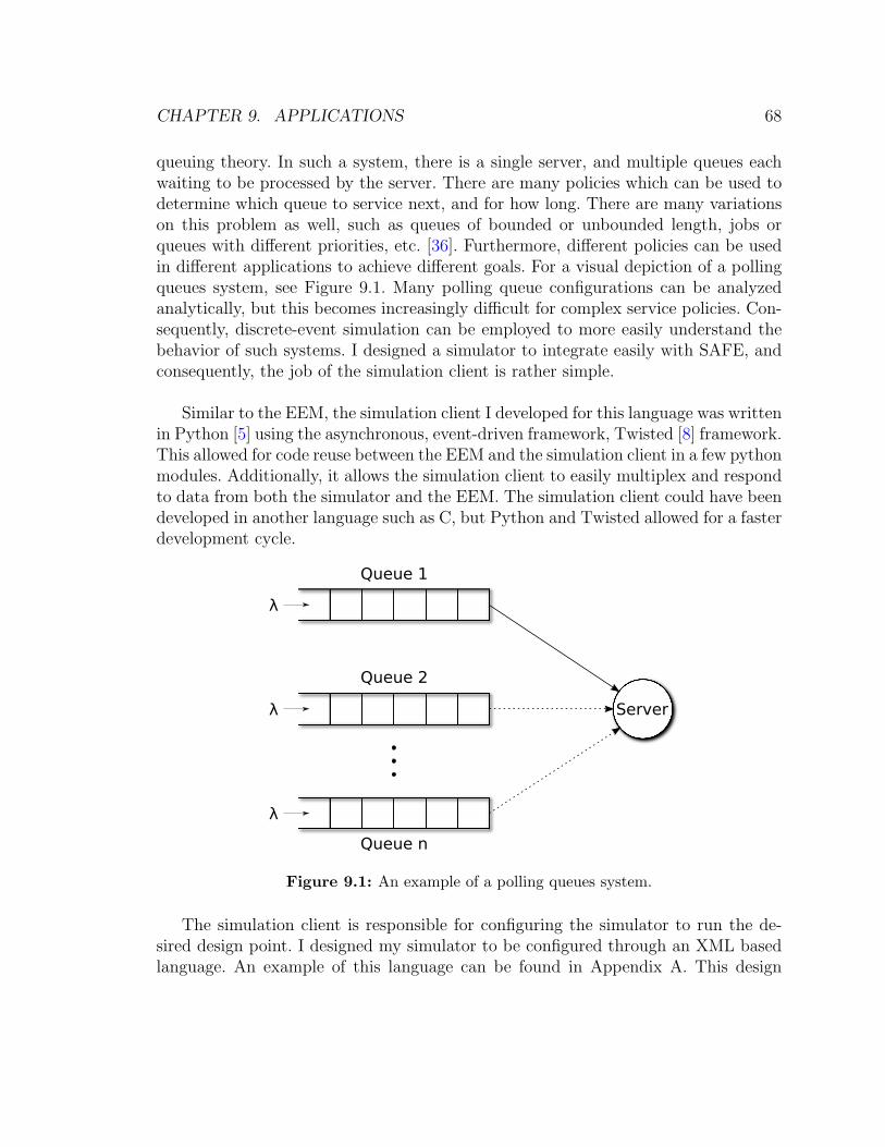
CHAPTER 9. APPLICATIONS 68
queuing theory. In such a system, there is a single server, and multiple queues eachwaiting to be processed by the server. There are many policies which can be used todetermine which queue to service next, and for how long. There are many variationson this problem as well, such as queues of bounded or unbounded length, jobs orqueues with different priorities, etc. [36]. Furthermore, different policies can be usedin different applications to achieve different goals. For a visual depiction of a pollingqueues system, see Figure 9.1. Many polling queue configurations can be analyzedanalytically, but this becomes increasingly difficult for complex service policies. Con-sequently, discrete-event simulation can be employed to more easily understand thebehavior of such systems. I designed a simulator to integrate easily with SAFE, andconsequently, the job of the simulation client is rather simple.
Similar to the EEM, the simulation client I developed for this language was writtenin Python [5] using the asynchronous, event-driven framework, Twisted [8] framework.This allowed for code reuse between the EEM and the simulation client in a few pythonmodules. Additionally, it allows the simulation client to easily multiplex and respondto data from both the simulator and the EEM. The simulation client could have beendeveloped in another language such as C, but Python and Twisted allowed for a fasterdevelopment cycle.
λ
λ
λ
Queue 2
Queue 1
Queue n
Server
Figure 9.1: An example of a polling queues system.
The simulation client is responsible for configuring the simulator to run the de-sired design point. I designed my simulator to be configured through an XML basedlanguage. An example of this language can be found in Appendix A. This design
CHAPTER 9. APPLICATIONS 69
allows for the EEM to generate the XML model for the simulation, and pass it to thesimulation client which can run it directly.
The simulation client must next spawn the simulation itself. In Twisted there is amethod called spawnProcess() which is a wrapper around the necessary system callsto spawn a new process. This can be used to spawn a new process from an executablein the file system, such as the simulator. At a lower level in the Twisted library, thisis implemented by calling fork() to spawn the new process, and exec() to replacethe process with the simulator. Once this has been done, the simulator can beginexecution and the simulation client returns to it’s select() loop to wait for the nextevent to occur.
The spawnProcess() method also creates three standard pipes to the simula-tion client: Standard Input (STDIN), Standard Output (STDOUT), and Standard Error(STDERR). In the spawnProcess() library, this is done with the system calls pipe() tocreate these pipes and dup() to move them to file descriptors 0, 1 and 2 respectively.Either STDOUT or STDERR would be sufficient to pass results from the simulator to thesimulation client; however, I created a new pipe on file descriptor 3 specifically forresults from the simulator such that logging messages do not get misinterpreted asresults. The simulator can then open this pipe using fdopen(3) and write to it withwrite().
The simulation client can then communicate with the simulator itself over thesepipes. A callback in the simulation client is installed to run whenever there is dataready to be read from the pipes from the simulator. In the simulator, when a job isserviced, its total wait time is computed, and that statistic is written to the pipe onfile descriptor 3. The simulation client can then send that result to the EEM using aResult message.
The last responsibility of the simulation client is to properly terminate the simula-tion when notified by the EEM. This is done by sending a signal, which the simulatorcan handle to terminate the simulation. In Twisted, this can be easily done by callingsendSignal() on the object abstracting the simulator process.
The simulation client developed to integrate with my simple polling queues sim-ulator demonstrates the basic functionalities that are required of a simulation client.Furthermore, when the simulator can be easily controlled by an external process thana simulation client can be developed relatively easily to allow the simulator to beused with SAFE. The development of a simulation client is made easier for futuresimulators in that they can follow the example set forward by this simulation client

CHAPTER 9. APPLICATIONS 70
implementation.
9.2 Case Study: ns-3
The previous simulation client demonstrates the simplest case of how a simulator canbe integrated with SAFE. However, not all discrete-event simulation engines can beintegrated this easily though with SAFE. This section describes the basics of how oneuses the popular network simulator ns-3 and the challenges associated with buildinga compatible simulation client.
9.2.1 ns-3 Architecture
Simulation models in ns-3 are encoded in C++ or Python scripts. These scripts relyheavily on the ns-3 core libraries and allow the simulation user to model the system ata high level. On the other hand, a simulation model cannot be encoded in a text-basedconfiguration file which the simulator accepts as input.
There is an additional module in ns-3 called ConfigStore which allows a staticns-3 simulation model to be configured through an XML based language. For ex-ample, the frequency at which wireless network nodes operate may be able to beconfigured through ConfigStore, but not the number of nodes in the simulation. Forexperiments which only vary attributes to simulation objects such as wireless fre-quency, ConfigStore can be used in conjunction with a constant simulation model.When the experiment must vary the simulation model, such as the number of nodesin the simulation, a new simulation script must be generated for each design point. Atthe Fall 2010 ns-3 developer’s meeting [11], there was discussion of possibly extendingConfigStore such that ns-3 models could be described in XML.
Another feature of ns-3 is that most tasks are executed using a software systemcalled waf [10], which claims to be similar to automake [1]. This helps the user incompiling and running simulation scripts in the right environment. To an automationtool like SAFE, this adds an additional level of complexity in that waf spawns a newprocess for the simulation process itself.
Most ns-3 users gather statistics from simulations by processing packet traces

CHAPTER 9. APPLICATIONS 71
which the simulator saves after execution. Another project under development, calledthe Data Collection Framework (DCF), funded under the same NSF grant as SAFE[20] seeks to ease the process of collecting data and statistics from within ns-3 simu-lation. The DCF should ease the process of gathering statistics from ns-3.
9.2.2 ns-3 Simulation Client
The ns-3 simulation client receives the simulation model from the EEM just as theprevious simulation client does. The challenge with ns-3 is that the simulator cannotalways be configured through XML. This introduces two use cases, one in which thens-3 simulation model must be generated in C++ or Python, and another in whichthe simulation can be configured using XML and ConfigStore. If the only levels beingvaried in the simulation model are attributes to different objects in the simulation(e.g. bandwidth) then the XML model generated by the EEM can simply be fed intoConfigStore and executed. In cases in which this is not sufficient, a C++ or Pythonbased simulation script can be generated from a template and executed [19].
The ns-3 simulation is spawned similarly to my previous simulator using thespawnProcess() method. The difference between the two simulators is that in ns-3spawnProcess() is called on waf which in turn spawns ns-3. Because ns-3 is a childprocess of waf, it shares the open file table with waf, and thus has access to the samepipes from the simulation client. This allows statistics to be computed, particularlyin the DCF, and written to the pipe on file descriptor 3. The DCF will also providemechanisms to tag results for different metrics, which will be sent along with theresult to the EEM for storage in the database.
The last complication of using SAFE with ns-3 is that calling signalProcess()
sends a signal to the waf process, not the simulator itself. The simulation client musttherefore terminate not only the waf process, but also all child processes of waf. Onceall of these processes have been terminated, the simulation client can request the nextsimulation.

CHAPTER 9. APPLICATIONS 72
Chapter Summary
This chapter discusses how SAFE can be used with two simulators. The first simulatordiscussed is a polling queues simulator which I developed to easily integrate withSAFE. The second simulator was ns-3 which posed several challenges to integratewith SAFE. The investigation of these two cases demonstrates the considerations onemust make to integrate with SAFE. Furthermore, they demonstrate the flexibility ofthe SAFE architecture in that it can be adapted for use with a few types of simulators.The next chapter concludes my thesis and describes areas for future work.

73
Chapter 10
Conclusions & Future Work
The complexity of the execution of proper simulation methodology has led to an over-all lack of credibility observed in recently published simulation articles. This problemcan be addressed through the automation of proper simulation workflow. SAFE buildsupon many of the features seen in previous automation tools to provide a frameworkwith which simulation users can conduct rigorous scientific simulation experiments.
Simulation automation enhances the usability of a simulator as well as the credi-bility of the simulation results. Users can configure their simulation through the XMLbased languages and execute their experiment with the assurance that the proper sim-ulation workflow will be applied. The execution of the simulations themselves requireno user interaction. Researchers can therefore focus on their science instead of theirsimulations.
SAFE’s extensible architecture loosely couples the EEM and the specifics of theimplementation of the simulator. SAFE can be made compatible with other discrete-event simulators by customizing a simulation client to the needs of the specific simu-lator. This gives SAFE a broad scope of application allowing simulation users in manyproblem domains to reap the benefits of the framework. It is important to note thatSAFE cannot necessarily be integrated with all discrete-event simulators due to thechallenges associated with setting up a design point and collecting results program-matically. For example, some proprietary simulators may be configured exclusivelythrough a Graphical User Interface (GUI) which cannot be easily controlled in thesimulation client. Simulators which can be easily configured through software using,for example, a configuration file can be more easily integrated with SAFE. Finally,

CHAPTER 10. CONCLUSIONS & FUTURE WORK 74
if a simulator is designed from the ground up to be used with SAFE, the challengesassociated with integrating with SAFE can be minimized as seen in Section 9.1.
SAFE has been released as open source software under a General Public License(GPL), and it will be packaged with ns-3 in future releases as part of the work con-ducted under Dr. Perrone’s recent NSF grant [20]. This will give the project visibilityto ns-3 users around the world and allow for the continued development of the soft-ware. Additionally, this visibility will hopefully promote the use of my frameworkwith other simulators.
My work on SAFE focuses primarily on its architecture and the execution of sim-ulation experiments. This work provides a framework upon which many new featuresand capabilities can be built. The follow are a few proposals for future research.
The user interfaces currently provided by SAFE demonstrate the possibilities ofthe architecture and the project, though they are rather simplistic. Future work couldbe done to enhance the usability of these user interfaces, or expose new features ofthe framework through these interfaces. For example, the web manager could beextended to provide more sophisticated analysis tools. Another project could be todevelop graphical user interfaces to help novice or intermediate users design theirsimulation experiments without needing to write XML.
For the entirety of this thesis, it has been assumed that individual simulationruns are run on a single processor. Many simulators, however, such as SWAN andns-3 can be run in parallel using MPI. An interesting area of future research is todevelop algorithms to determine how many of the available processors on a machineshould be employed per simulation run. For example, if a system has eight cores, itcan run eight simultaneous simulations, or it can run a single simulation across alleight processing cores. A future area of research could investigate how to allocatecomputational resources either by the EEM or the simulation client to speed up thesimulation experiment.
SAFE’s EEM is currently only capable of managing a single simulation at a time.There are many applications in which it could be useful for the EEM to managemultiple experiments. For example, in the classroom it could be useful for a professorto setup a single EEM and allow students to create and execute their own simula-tion experiments. This introduces additional complexity in the EEM to determinewhich simulation in which experiment to dispatch. There could be many algorithmsto determine how and when to dispatch design points to simulation clients to achievebetter performance.

CHAPTER 10. CONCLUSIONS & FUTURE WORK 75
An interesting application of this functionality is the classroom. A single EEMcould be run by an instructor and every student could be allowed to create their ownexperiments. In an educational setting this streamlined workflow can make simulationmore accessible particularly in an undergraduate course. Furthermore, the computa-tional resources available for running simulations could be more evenly distributedby the EEM to students in the course.
As the SAFE project evolves, I expect that new applications will spur the devel-opment of additional plugins so that the framework’s functionalities are expandedto meet the needs of its users. This will allow SAFE to facilitate scientific achieve-ments, in addition to being the subject of future scientific advancements in simulationautomation, credibility and usability.

76
References
[1] Automake. Available at <http://www.gnu.org/software/automake/> [Ac-cessed April 8, 2011].
[2] Cheetah – the Python-powered template engine. Available at<http://www.cheetahtemplate.org> [Accessed March 29, 2011].
[3] MATLAB – the language of technical computing. Available at<http://www.mathworks.com/products/matlab/> [Accessed April 17, 2011].
[4] GNU octave. Available at <http://www.gnu.org/software/octave/> [Ac-cessed April 17, 2011].
[5] Python. Available at <http://python.org> [Accessed September 1, 2010].
[6] The R project for statistical computing. Available at<http://www.r-project.org/> [Accessed April 17, 2011].
[7] SciPy: Scientfic tools for Python. Available at <http://www.scipy.org/> [Ac-cessed April 17, 2011].
[8] Twisted. Available at <http://twistedmatrix.com/> [Accessed April 8, 2011].
[9] XML Technologies, World Wide Web Consortium. Available at<http://www.w3.org/standards/xml/> [Accessed April 17, 2011].
[10] waf: The meta build system. Available at <http://code.google.com/p/waf/>[Accessed April 8, 2011].
[11] ns-3 developers meeting, November 2010. Washington D.C., U.S.A.
[12] Matteo Maria Andreozzi, Giovanni Stea, and Carlo Vallati. A framework forlarge-scale simulations and output result analysis with ns-2. In Proc. of the 2ndIntl. Conf. on Simulation Tools and Techniques (SIMUTools ’09), 2009.

REFERENCES 77
[13] Jerry Banks, John S. Carson, Barry L. Nelson, and David M. Nicol. Discrete-Event System Simulation. Prentice Hall, fourth edition, 2004.
[14] Adam L. Beberg, Daniel L. Ensign, Guha Jayachandran, Siraj Khaliq, and Vi-jay S. Pande. Folding@Home: Lessons from eight years of volunteer distributedcomputing. In Proceedings of the 2009 IEEE International Symposium on Paral-lel&Distributed Processing, pages 1–8, Washington, DC, USA, 2009. IEEE Com-puter Society. ISBN 978-1-4244-3751-1. doi: 10.1109/IPDPS.2009.5160922. URLhttp://portal.acm.org/citation.cfm?id=1586640.1587707.
[15] Claudio Cicconetti, Enzo Mingozzi, and Giovanni Stea. An integrated frame-work for enabling effective data collection and statistical analysis with ns-2. InProceedings of the 2006 workshop on ns-2: the IP network simulator, WNS2 ’06,2006.
[16] Ramez Elmasri and Shamkant B. Navathe. Fundamentals of Database Systems.Addison Wesley, fifth edition, March 2006.
[17] Roy Thomas Fielding. Architectural styles and the design of network-based soft-ware architectures. PhD thesis, University of California, Irvine, 2000.
[18] Richard Fujimoto and David Nicol. State of the art in parallel simulation. InProceedings of the 24th Winter Simulation Conference, WSC ’92, pages 246–254,New York, NY, USA, 1992. ACM. ISBN 0-7803-0798-4.
[19] Andrew H. Hallagan. The design of an XML-based model description languagefor wireless ad-hoc networks simulations. Undergraduate Honors Thesis, BucknellUniversity, Lewisburg, PA, 2011.
[20] Thomas Henderson, L. Felipe Perrone, and George Ri-ley. Frameworks for ns-3, 2010. Available at<http://www.nsf.gov/awardsearch/showAward.do?AwardNumber=0958142>
[Accessed September 1, 2010].
[21] John L. Hennessy and David A. Patterson. Computer Architecture: A Quantita-tive Approach. Morgan Kaufmann, 4th edition, 2006.
[22] J. Himmelspach, R. Ewald, and A.M. Uhrmacher. In Proceedings of the 40thWinter Simulation Conference.
[23] Christopher J. Kenna. An experiment design framework for the Simulator ofWireless Ad Hoc Networks. Undergraduate Honors Thesis, Bucknell University,Lewisburg, PA, 2008.

REFERENCES 78
[24] Michael Kifer, Arthur Bernstein, and Philip M. Lewis. Database Systems: AnApplication-Oriented Approach. Addison Wesley, 2nd edition, March 2005.
[25] Stuart Kurkowski, Tracy Camp, and Michael Colagrosso. MANET simulationstudies: the incredibles. SIGMOBILE Mob. Comput. Commun. Rev., 9(4):50–61,2005.
[26] Averill M. Law. Simulation Modeling and Analysis. McGraw-Hill, 3rd edition,2000.
[27] S. Leye, J. Himmelspach, M. Jeschke, R. Ewald, and A.M. Uhrmacher. A grid-inspired mechanism for coarse-grained experiment execution. In Distributed Sim-ulation and Real-Time Applications, 2008. DS-RT 2008. 12th IEEE/ACM Inter-national Symposium on, pages 7 –16, oct. 2008. doi: 10.1109/DS-RT.2008.33.
[28] Krzysztof Pawlikowski. Akaroa2: Exploiting network computing by distributingstochastic simulation. In Proc. of the 1999 European Simulation Multiconference,pages 175–181, Warsaw, Poland, 1999.
[29] Krzysztof Pawlikowski. Do not trust all simulation studies of telecommunicationnetworks. In Proceedings of the International Conference on Information Net-working, Networking Technologies for Enhanced Internet Services, pages 899–908, 2003.
[30] L. Felipe Perrone, Claudio Cicconetti, Giovanni Stea, and Bryan C. Ward. Onthe automation of computer network simulators. In Proceedings of the 2nd In-ternational Conference on Simulation Tools and Techniques.
[31] L.F. Perrone, C.J. Kenna, and B.C. Ward. Enhancing the credibility of wirelessnetwork simulations with experiment automation. In Proc. of the 2008 IEEE In-ternational Conference on Wireless & Mobile Computing, Networking and Com-munications, WiMob ’08), pages 631–637, 2008.
[32] Larry L. Peterson and Bruce S. Davie. Computer Networks: A Systems Approach.Morgan Kaufmann, 3rd edition, 2003.
[33] Dragan Savic, Matevz Pustisek, and Francesco Potortı. A tool for packaging andexchanging simulation results. In Proc. of the First International Conferenceon Performance Evaluation Methodologies and Tools, VALUETOOLS ’06, Pisa,Italy, 2006. ACM.
[34] Douglas C. Schmidt. Reactor: an object behavioral pattern for concurrentevent demultiplexing and event handler dispatching, pages 529–545. ACM

REFERENCES 79
Press/Addison-Wesley Publishing Co., New York, NY, USA, 1995. ISBN 0-201-60734-4. URL http://portal.acm.org/citation.cfm?id=218662.218705.
[35] Abraham Silverschatz, Peter B. Galvin, and Greg Gagne. Operating SystemConcepts with Java. Wiley, 7th edition, 2006.
[36] Hideaki Takagi. Queuing analysis of polling models. ACM Comput. Surv., 20:5–28, March 1988. ISSN 0360-0300.
[37] Andrew S. Tanenbaum. Computer Networks. Prentice Hall, fourth edition, 2002.

Part IV
Appendices
80

81
Appendix A
Polling Queues Example XMLConfiguration
<simulation>
<manager>
<seed>1027</seed>
<transient>10</transient>
<termination>
<time>100</time>
<response>2</response>
<min_samples>20</min_samples>
</termination>
</manager>
<server>
<service>
<random_variable>
<distribution>gauss</distribution>
<mean>5</mean>
<stdev>1</stdev>
</random_variable>
</service>
<switch_queue>
<random_variable>
<distribution>gauss</distribution>
<mean>1</mean>

APPENDIX A. POLLING QUEUES EXAMPLE XML CONFIGURATION 82
<stdev>0.1</stdev>
</random_variable>
</switch_queue>
<next_job_time>
<random_variable>
<distribution>gauss</distribution>
<mean>1</mean>
<stdev>0.5</stdev>
</random_variable>
</next_job_time>
<policy><model>longest</model></policy>
</server>
<queues>
<count>5</count>
<iat>
<random_variable>
<distribution>exponential</distribution>
<lambda>0.166666</lambda>
</random_variable>
</iat>
<length>10</length>
</queues>
</simulation>
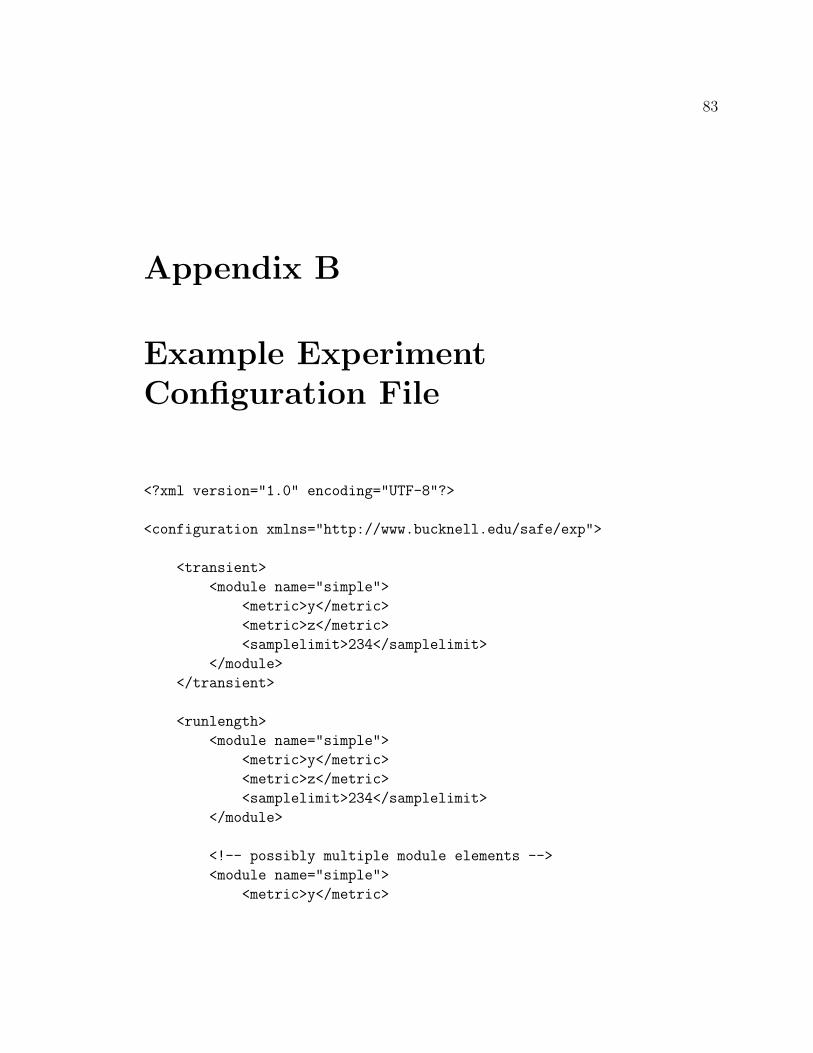
83
Appendix B
Example ExperimentConfiguration File
<?xml version="1.0" encoding="UTF-8"?>
<configuration xmlns="http://www.bucknell.edu/safe/exp">
<transient>
<module name="simple">
<metric>y</metric>
<metric>z</metric>
<samplelimit>234</samplelimit>
</module>
</transient>
<runlength>
<module name="simple">
<metric>y</metric>
<metric>z</metric>
<samplelimit>234</samplelimit>
</module>
<!-- possibly multiple module elements -->
<module name="simple">
<metric>y</metric>

APPENDIX B. EXAMPLE EXPERIMENT CONFIGURATION FILE 84
<metric>z</metric>
<samplelimit>234</samplelimit>
</module>
</runlength>
<parser>
<expparser>expparser.py</expparser>
<modelparser>modparse.py</modelparser>
</parser>
<options>
<simulator>ns3</simulator>
<version>3.9</version>
</options>
</configuration>

85
Appendix C
Example Cheetah Template
<simulation>
<manager>
<seed>1027</seed>
<transient>10</transient>
<termination>
<time>100</time>
<response>2</response>
<min_samples>20</min_samples>
</termination>
</manager>
<server>
<service>
<random_variable>
<distribution>gauss</distribution>
<mean>$service_mean</mean>
<stdev>$service_stder</stdev>
</random_variable>
</service>
<switch_queue>
<random_variable>
<distribution>gauss</distribution>
<mean>0</mean>
<stdev>0</stdev>
</random_variable>

APPENDIX C. EXAMPLE CHEETAH TEMPLATE 86
</switch_queue>
<next_job_time>
<random_variable>
<distribution>gauss</distribution>
<mean>2</mean>
<stdev>0.5</stdev>
</random_variable>
</next_job_time>
<policy>
<model>longest</model>
</policy>
</server>
<queues>
<count>$queue_counts</count>
<iat>
<random_variable>
<distribution>exponential</distribution>
<lambda>0.166666</lambda>
</random_variable>
</iat>
<length>$queue_length</length>
</queues>
</simulation>
Related Documents