A forward-backward Monte Carlo method for solving influence diagrams

International Journal of Approximate Reasoning42 (2006) 119–135

www.elsevier.com/locate/ijar

A forward–backward Monte Carlo methodfor solving influence diagrams

Andres Cano, Manuel Gomez *, Serafın Moral

Computer Science Department, E.T.S.I. Informatica, University of Granada, Granada 18071, Spain

Accepted 1 October 2005Available online 4 November 2005

Abstract

Although influence diagrams are powerful tools for representing and solving complex decision-making problems, their evaluation may require an enormous computational effort and this is a pri-mary issue when processing real-world models. We shall propose an approximate inference algo-rithm to deal with very large models. For such models, it may be unfeasible to achieve an exactsolution. This anytime algorithm returns approximate solutions which are increasingly refined ascomputation progresses, producing knowledge that offers insight into the decision problem.� 2005 Elsevier Inc. All rights reserved.

Keywords: Influence diagrams; Monte Carlo simulation; Classification trees

1. Introduction

Influence diagrams (IDs) [11] are a very compact representation of decision problems.IDs include explicit representation for the basic elements of this kind of problem: uncer-tainty about the state of the world, alternatives under the decision maker�s control, andpreferences. There are several methods for evaluating IDs. While some of these transformIDs into secondary structures, others evaluate them directly: [11,27,7,31,26,28,25,19,12,

0888-613X/$ - see front matter � 2005 Elsevier Inc. All rights reserved.

doi:10.1016/j.ijar.2005.10.009

* Corresponding author. Tel.: +34 958 240465; fax: +34 958 243317.E-mail addresses: [email protected] (A. Cano), [email protected] (M. Gomez), [email protected]

(S. Moral).

120 A. Cano et al. / Internat. J. Approx. Reason. 42 (2006) 119–135

32,18]. There is a review of asymmetric decision problems in [1], although more recentwork can be found in [21,8,13].

Nevertheless, all of these offer a decision function for each decision variable. This deci-sion function is defined on the set of relevant variables for every decision and indicates thepreferred alternative (that of maximum expected utility) for each configuration of valuesfor the relevant variables. The problem arises when the number of relevant variables for adecision is very large. In such cases, IDs become intractable, as the number of configura-tions for every decision function is unmanageable. The problem lies not only in computingthe values required for each decision function, but also in representing the function itself.

Approximate methods have been proposed to cope with this difficulty. While some ofthese use simulation in order to approximate the decision functions (for example [15,2,6]),others build these functions by means of an incremental procedure which adds the consid-ered variables as the algorithm progresses according to their relevance (the expected valueof improvement gained when the variable is added) [10].

Our proposed method could possibly be an intermediate solution between the last twoapproaches mentioned above. We use simulation to obtain approximate decision func-tions, but it is not necessary to sample the whole state space of the relevant variablesfor the decisions exhaustively, as in [6]. Although the set of relevant variables is minimizedin this work (as described in [20]), this set may be large enough to make the decision prob-lem intractable. Horsch�s work [10] does not use simulation. The approximation isobtained by making decision functions on an incremental procedure. The relevant vari-ables are added one at a time in an attempt to maximize the expected value of improve-ment in utility.

The main objective of the method presented in this paper is to obtain as much knowl-edge as possible about very complex decision problems, while recognizing that an exactsolution for them may not be affordable. It is conceived as an anytime algorithm merelybecause we always have approximate decision functions which become increasingly refinedas new computations are carried out. The knowledge is therefore added incrementally todecision functions. The procedure is organized so as to obtain new information with theleast possible effort.

This is possible despite the evaluation method used for computation. We only need oneevaluation method which is able to compute the expected utility for an ID given knowl-edge about several of its variables. Moreover, the procedure can take into account the con-straints about the ID variables (asymmetries), thereby avoiding considering restrictedconfigurations and using this information to simplify computations as far as possible.

2. Preliminaries

IDs are directed acyclic graphs with three types of nodes: decision nodes (mutuallyexclusive actions which the decision maker must choose from); chance nodes (events thatthe decision maker cannot control); and utility nodes (representing decision maker prefer-ences). Links represent dependencies: probabilistic for links to chance nodes, informa-tional for links to decision nodes (states for decision parents are known before thedecision is taken), and functional for links to value nodes. In order to explain the notationand the algorithm better, an ID is used: the buyer car problem (see [30], Fig. 1). The size ofthis ID does not favor the use of this algorithm on it; it is included for reasons of clarityduring explanations about its main features. The existence of one value node should not be

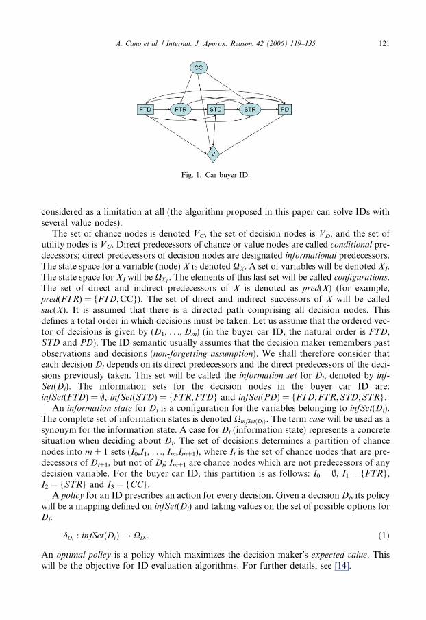
Fig. 1. Car buyer ID.

A. Cano et al. / Internat. J. Approx. Reason. 42 (2006) 119–135 121

considered as a limitation at all (the algorithm proposed in this paper can solve IDs withseveral value nodes).

The set of chance nodes is denoted VC, the set of decision nodes is VD, and the set ofutility nodes is VU. Direct predecessors of chance or value nodes are called conditional pre-decessors; direct predecessors of decision nodes are designated informational predecessors.The state space for a variable (node) X is denoted XX. A set of variables will be denoted XI.The state space for XI will be XX I . The elements of this last set will be called configurations.The set of direct and indirect predecessors of X is denoted as pred(X) (for example,pred(FTR) = {FTD,CC}). The set of direct and indirect successors of X will be calledsuc(X). It is assumed that there is a directed path comprising all decision nodes. Thisdefines a total order in which decisions must be taken. Let us assume that the ordered vec-tor of decisions is given by (D1, . . ., Dm) (in the buyer car ID, the natural order is FTD,STD and PD). The ID semantic usually assumes that the decision maker remembers pastobservations and decisions (non-forgetting assumption). We shall therefore consider thateach decision Di depends on its direct predecessors and the direct predecessors of the deci-sions previously taken. This set will be called the information set for Di, denoted by inf-

Set(Di). The information sets for the decision nodes in the buyer car ID are:infSet(FTD) = ;, infSet(STD) = {FTR,FTD} and infSet(PD) = {FTD,FTR,STD,STR}.

An information state for Di is a configuration for the variables belonging to infSet(Di).The complete set of information states is denoted XinfSetðDiÞ. The term case will be used as asynonym for the information state. A case for Di (information state) represents a concretesituation when deciding about Di. The set of decisions determines a partition of chancenodes into m + 1 sets (I0,I1, . . ., Im,Im+1), where Ii is the set of chance nodes that are pre-decessors of Di+1, but not of Di; Im+1 are chance nodes which are not predecessors of anydecision variable. For the buyer car ID, this partition is as follows: I0 = ;, I1 = {FTR},I2 = {STR} and I3 = {CC}.

A policy for an ID prescribes an action for every decision. Given a decision Di, its policywill be a mapping defined on infSet(Di) and taking values on the set of possible options forDi:

dDi : infSetðDiÞ ! XDi . ð1Þ

An optimal policy is a policy which maximizes the decision maker�s expected value. Thiswill be the objective for ID evaluation algorithms. For further details, see [14].

122 A. Cano et al. / Internat. J. Approx. Reason. 42 (2006) 119–135

3. Algorithm

When infSet(Di) is very large, it may be impossible to compute or even represent thedecision function for Di. Although an exact solution may be unfeasible, it is interestingto gain some insight into system proposals (at least those relating to the most probablecases). The Monte Carlo algorithm presented in this paper is designed to cope with suchsituations. It could be seen as a last resort algorithm when everything else fails. Section 3.1offers a general overview of this algorithm which is formally described in Section 3.2.

3.1. General overview

The basic idea of the algorithm is that if infSet(Di) is very large (this may be true for oneor several decision nodes), then the probability of most of the Di information states occur-ring may be very small. Some variables may therefore be irrelevant, having a very small (oreven no) impact on decision functions. Some of these variables can be detected using thegraph for the problem (see [20,24]), but in this paper they will be determined with anapproximate computation. This computation depends on the numerical values of proba-bilities and utilities. This is not simple because the probabilities and utilities of the infor-mation states for a decision Di depends on the remaining decisions.

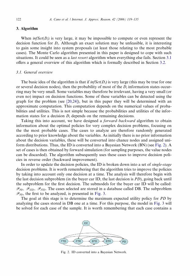
Taking this into account, we have designed a forward–backward algorithm to obtaininformation about the optimal policies for very complex decision problems, focusing onthe the most probable cases. The cases to analyze are therefore randomly generatedaccording to prior knowledge about the variables. As initially there is no prior informationabout the decision variables, these will be converted into chance nodes and assigned uni-form distributions. Thus, the ID is converted into a Bayesian Network (BN) (see Fig. 2). Aset of cases is then obtained by forward simulation (for sampling purposes, the value nodescan be discarded). The algorithm subsequently uses these cases to improve decision poli-cies in reverse order (backward improvement).

In order to update the decision policies, the ID is broken down into a set of single-stagedecision problems. It is worth remembering that the algorithm tries to improve the policiesby taking into account only one decision at a time. The analysis will therefore begin withthe last decision subproblem (in the buyer car ID, the last decision is PD), going back untilthe subproblem for the first decision. The submodels for the buyer car ID will be called:PPD; PSTD; PFTD. The cases selected are stored in a database called DB. The subproblemPPD, the first to be analyzed, is presented in Fig. 3.

The goal at this stage is to determine the maximum expected utility policy for PD byanalyzing the cases stored in DB one at a time. For this purpose, the model in Fig. 3 willbe solved for each case of the sample. It is worth remembering that each case contains a

Fig. 2. ID converted into a Bayesian Network.

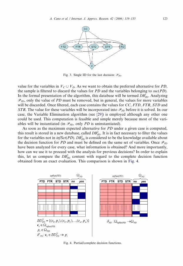
Fig. 3. Single ID for the last decision: PPD.

A. Cano et al. / Internat. J. Approx. Reason. 42 (2006) 119–135 123

value for the variables in VC [ VD. As we want to obtain the preferred alternative for PD,the sample is filtered to discard the values for PD and the variables belonging to suc(PD).In the formal presentation of the algorithm, this database will be termed DB1

PD. AnalyzingPPD, only the value of PD must be removed, but in general, the values for more variableswill be discarded. Once filtered, each case contains the values for CC, FTD, FTR, STD andSTR. The value for these variables will be incorporated into PPD before it is solved. In ourcase, the Variable Elimination algorithm (see [29]) is employed although any other onecould be used. This computation is feasible and simple merely because most of the vari-ables will be instantiated (in PPD, only PD is uninstantiated).

As soon as the maximum expected alternative for PD under a given case is computed,this result is stored in a new database, called DB2

PD. It is in fact necessary to filter the valuesfor the variables not in infSet(PD). DB2

PD is considered to be the knowledge available aboutthe decision function for PD and must be defined on the same set of variables. Once PPD

have been analyzed for every case, what information is obtained? And more importantly,how can we use it to proceed with the analysis for previous decisions? In order to explainthis, let us compare the DB2

PD content with regard to the complete decision functionobtained from an exact evaluation. This comparison is shown in Fig. 4.

Fig. 4. Partial/complete decision functions.

124 A. Cano et al. / Internat. J. Approx. Reason. 42 (2006) 119–135

The left-hand side of Fig. 4 shows the available information after solving PPD for theshaded cases (rows). It must be considered that if all the cases are analyzed, then DB2

PD willbe complete. d0PD would therefore be the same as the decision function computed with anexact algorithm (right-hand side of Fig. 4). In the general case, only some informationstates are available and d0PD will be a partial evaluation of dPD on this reduced set of infor-mation states. At this point, only the policy for PD is optimized. The alternatives for theprevious decisions were carried out randomly. It is now time to improve them, but howshould this be done from the already computed partial decision function d0PD? The solutionis to use d0PD as if it were complete. Intuitively, this means dealing with new cases usingwhat is already known. In order to generalize d0PD to act as a complete decision function,a classifier is learned from DB2

PD, where PD is the class variable and the variables in inf-

Set(PD) are the attributes. More information about the learning method for this classifiercan be found in Sections 3.2 and 4.3.

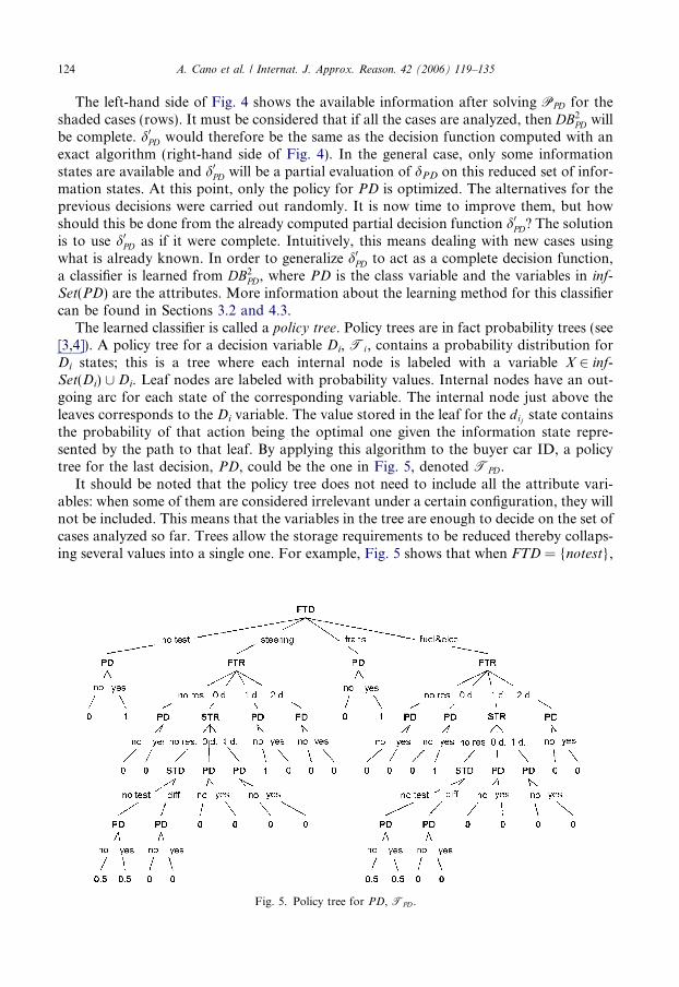
The learned classifier is called a policy tree. Policy trees are in fact probability trees (see[3,4]). A policy tree for a decision variable Di, Ti, contains a probability distribution forDi states; this is a tree where each internal node is labeled with a variable X 2 inf-

Set(Di) [ Di. Leaf nodes are labeled with probability values. Internal nodes have an out-going arc for each state of the corresponding variable. The internal node just above theleaves corresponds to the Di variable. The value stored in the leaf for the dij state containsthe probability of that action being the optimal one given the information state repre-sented by the path to that leaf. By applying this algorithm to the buyer car ID, a policytree for the last decision, PD, could be the one in Fig. 5, denoted TPD.

It should be noted that the policy tree does not need to include all the attribute vari-ables: when some of them are considered irrelevant under a certain configuration, they willnot be included. This means that the variables in the tree are enough to decide on the set ofcases analyzed so far. Trees allow the storage requirements to be reduced thereby collaps-ing several values into a single one. For example, Fig. 5 shows that when FTD = {notest},

Fig. 5. Policy tree for PD, TPD.

A. Cano et al. / Internat. J. Approx. Reason. 42 (2006) 119–135 125

the preferred alternative for PD is yes, regardless of the values for the remaining vari-ables. The complete decision function has 192 values, but only 32 values are required torepresent the information obtained by learning in DB2

PD. Some configurations are notallowed, as they are related to asymmetries: for example, if FTD = {steering}, then thevalue for FTR cannot be noresult. This policy tree generalizes d0PD, making it possible toact as an approximate version of the complete decision function. Let us suppose thatthe configuration {FTD = steering,FTR = 1defect,STD = notest,STR = noresult} doesnot belong to DB2

PD. The policy for this case is given by the information gathered fromthe analyzed sample (as though decision makers only had information obtained from theirown experience). How can the policy for this new configuration be obtained? The valuesfor the variables in it are used to select a path through the tree, going from the root of thetree to the proposal: PD = no (do not purchase the car).

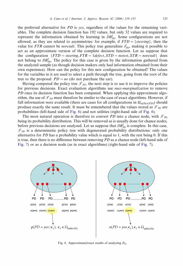
Having computed the policy tree TPD, the next step is to use it to improve the policiesfor previous decisions. Exact evaluation algorithms use max-marginalization to removePD once its decision function has been computed. When applying this approximate algo-rithm, the use of TPD must therefore be similar to the case of exact algorithms. However, iffull information were available (there are cases for all configurations in XinfSet(PD)) shouldproduce exactly the same result. It must be remembered that the values stored at TPD areprobabilities (left-hand side of Fig. 6) and not utilities (right-hand side of Fig. 6).

The most natural operation is therefore to convert PD into a chance node, with TPD

being its probability distribution. This will be removed as is usually done for chance nodes,before previous decisions are analyzed. Let us suppose that DB2

PD is complete. In this case,TPD is a deterministic policy tree with degenerated probability distributions: only onealternative for PD has a probability value which is equal to 1, with the rest being 0. If thisis true, then there is no difference between removing PD as a chance node (left-hand side ofFig. 7) or as a decision node (as in exact algorithms) (right-hand side of Fig. 7).

Fig. 6. Approximate/exact results of analyzing Dm.

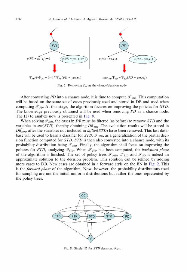
Fig. 7. Removing Dm as the chance/decision node.

126 A. Cano et al. / Internat. J. Approx. Reason. 42 (2006) 119–135

After converting PD into a chance node, it is time to compute TSTD. This computationwill be based on the same set of cases previously used and stored in DB and used whencomputing TPD. At this stage, the algorithm focuses on improving the policies for STD.The knowledge previously obtained will be used when removing PD as a chance node.The ID to analyze now is presented in Fig. 8.

When solving PSTD, the cases in DB must be filtered (as before) to remove STD and thevariables in suc(STD), thereby obtaining DB1

STD. The evaluation results will be stored inDB2

STD, after the variables not included in infSet(STD) have been removed. This last data-base will be used to learn a classifier for STD, TSTD, as a generalization of the partial deci-sion function computed for STD. STD is then also converted into a chance node, with itsprobability distribution being TSTD. Finally, the algorithm shall focus on improving thepolicies for FTD, analyzing PFTD. When TFTD has been computed, the backward phase

of the algorithm is finished. The set of policy trees TFTD, TSTD and TPD is indeed anapproximate solution to the decision problem. This solution can be refined by addingmore cases to DB. New cases are obtained in a forward style on the BN in Fig. 2. Thisis the forward phase of the algorithm. Now, however, the probability distributions usedfor sampling are not the initial uniform distributions but rather the ones represented bythe policy trees.

Fig. 8. Single ID for STD decision: PSTD.

A. Cano et al. / Internat. J. Approx. Reason. 42 (2006) 119–135 127

In summary, this algorithm breaks down the ID into a set of single-decision problems.Each problem Pi comes from changing the remaining decision nodes Dj, j 5 i, into chancenodes with Tj being the conditional probability of Dj. This is related to the policy network

(see [22]). This article explains how an ID can be transformed into a Bayesian networkgiven a set of policies fT1; . . . ;Tmg. One basic assumption of our approach is that forany information state for Di, it is possible to find the optimal option in problem Pi. Thiscomputation can easily be carried out: most of the variables will be instantiated and thereis only one decision node. In our experimental work, this is done with an exact algorithm,but if the single decision problems are too complex, it is possible to apply an approximatealgorithm, such as the one by [8], or a Monte Carlo algorithm as explained in [6].

3.2. Algorithm

Taking the elements of the previous section as a starting point, we shall describe ouralgorithm. At any given time, we shall have a vector of policies for the decision nodes.These policies will be represented by policy trees: ðT1; . . . ;TmÞ. Initially, all the policieswill be completely random: Ti will be a tree which contains the uniform distributionfor Di states.

The algorithm starts by using the policy network associated to the problem and policiesðT1; . . . ;TmÞ to simulate a sample with values for all the variables with the Logic Sam-pling procedure ([9]). This sample will be called the full database and denoted as DB.The size of the sample will be a fixed parameter N. Each register of the database will con-tain values for all the variables: (xo,d1,x1, . . .,dm,xm), where xi is a possible value of chancevariables Xi, and dj is a possible option of Dj. DB contains the cases under analysis at eachstage of the algorithm.

For each decision variable, Di, we will consider two databases: DB1i and DB2

i . The firstone, DB1

i , is obtained from DB including the variables (and their values) to instantiatewhen analyzing Pi. This database is obtained by removing the variables belonging tosuc(Di). The second one, DB2

i , is used to learn a classifier. This last one is obtained fromDB1

i by completing each register with the Di state maximizing the expected utility in prob-lem Pi and removing the variables not present in infSet(Di). The value for Di is completedin the registers by solving the decision problem, which was assumed to be feasible. Whenthe cases in DB1

i are evaluated then a classification tree T0i is induced from DB2

i .The procedure is repeated until a policy tree T0

i has been computed for every decision.The set of policy trees offers an approximate solution to the complete ID. Nevertheless,these policies may be refined by adding more knowledge. This requires obtaining morecases, as before. Now, however, the sampling for decision nodes is not a blind selectionof alternatives (with a uniform distribution) and the best alternative is selected based onactual information (the sampling distribution for Di is T0

i).The new cases will be stored in DB (where previously analyzed cases are also stored).

New computations must be carried out with these cases, obtaining new policy treesT00

1; . . . ;T00m to replace T0

1; . . . ;T0m. This iterative procedure is followed repeatedly until

K iterations have been performed (we shall later consider other alternative stoppingprocedures).

The sampling procedure can be easily modified to consider the asymmetries of the deci-sion problem (if it is asymmetric). The use of numerical trees to quantify constraints isexplained in [8]. The combination of these numerical trees with the current policy trees

128 A. Cano et al. / Internat. J. Approx. Reason. 42 (2006) 119–135

avoids cases being obtained which are related to constrained configurations, thereby sim-plifying the set of cases to analyze and focusing the algorithm on valid configurations.Moreover, it would be possible to add cases to DB with non-random procedures. Thiscould be interesting when some low probability cases are of special interest.

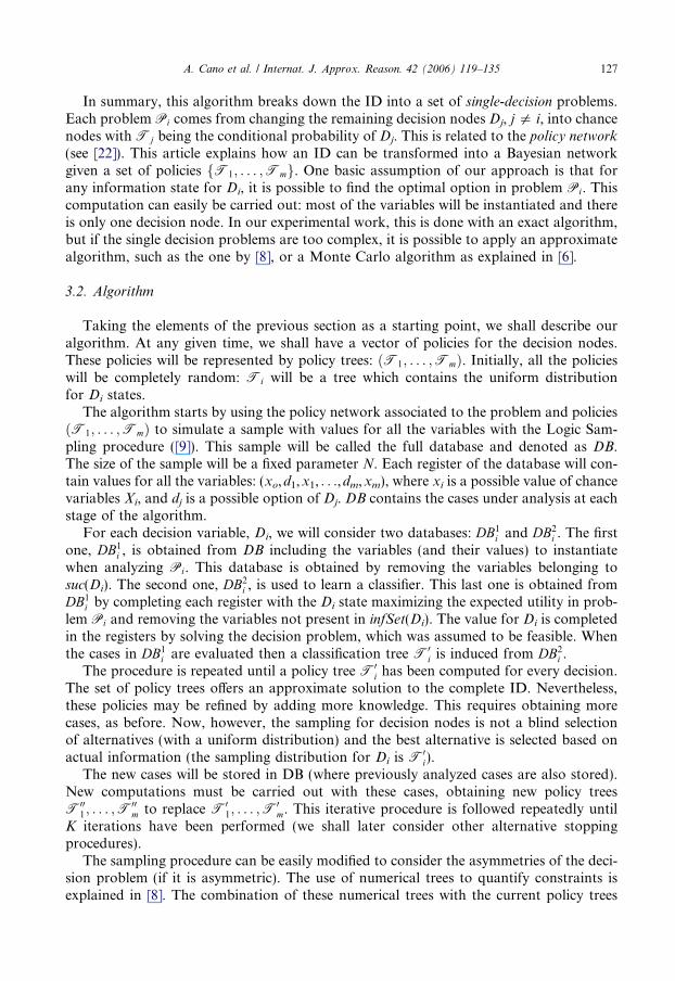
Having presented the basic ideas, we can give a formalized description of the algorithm:

1.Compute initial random policies ðT1; . . . ;TmÞ2.For k = 1 to K do steps 3–8

3.Obtain a database DB in the policy network for policies

ðT1; . . . ;TmÞ by Logic Sampling

4.For i = m down to 1 do steps 5–7

5.Compute database DB1i

6.Complete each register of DB1i with optimal decision of Di in Pi

computing database DB2i

7.Compute new random policy T0i inducing a classification tree

in DB2i ; Di is the class variable and the predicting attributes

are the other variables.

8.Replace ðT1; . . . ;TmÞ by ðT01; . . . ;T0

mÞ9.Output:deterministic version of ðT1; . . . ;TmÞ as the optimal set of

policies for the problem.

Line 3 is the forward step, and the loop comprising lines 4–7 is the backward step.The procedure for computing T 0i is based on classical methods for obtaining a classifi-

cation tree, where the class variable is Di in database DB2i . There are several procedures for

building classification trees. In this paper, we shall follow the C4.5 procedure [23] and amethod based on information gain where probabilities are estimated with Laplace correc-tion (as proposed by [5]). If we are in a leaf that is compatible with n registers in databaseDB2

i , the number of options of Di is si, and the number of times that the state dij appears inthese registers is rj, then the probability of dij in this leaf is:

rj þ 1

nþ si. ð2Þ

Only at the end of the iterations is a deterministic version of the policies computed byselecting the option with the greatest probability for each leaf. At intermediate steps, wekeep the random nature of the decisions, estimating their probabilities with this correction.This is the basic framework. There are certain variants and modifications which we haveconsidered. In the following sections, we shall describe additional details.

4. Additional details

4.1. Accumulative databases

The full database DB does not discard the cases used in previous iterations. This meansthat knowledge about new cases is incrementally added to the decision functions, and sothe approximations will be improved step by step. The set of cases generated for an iter-ation and stored in DB will be used to compute DB1

j . The results of evaluating Pj for allthe previous cases are kept in DB2

j . The computation of DB2j is different in the last decision

A. Cano et al. / Internat. J. Approx. Reason. 42 (2006) 119–135 129

Dm. Once a case has been evaluated for Pm, it is stored in DB2m and it will require no further

computation. It is worth remembering that Pm does not receive information from previousdecisions. Therefore, when DB1

m contains a case of the sample which has already been eval-uated, there is no need for further computation: the result is obtained from DB2

m and willbe stored as a new register in that database. The same does not hold for the other decisionssimply because T0

m may differ from Tm. The set of decision problems at the current iter-ation will therefore be different to the problems from the previous ones. It is then necessaryto recompute the optimal policy even for the cases of previous iterations.

4.2. Stopping criteria

In the current version of the algorithm, we define a fixed number of iterations as theparameter K. The consideration about accumulative databases, however, may also be usedin future versions. The following conditions may be considered, either individually orjointly:

• There are several iterations where no new cases are added to DB. In such case, theseiterations do not represent an important contribution to the refinement process. Thissituation could suggest that the algorithm has already considered the set of possibleconfigurations with a high probability (the remainder would have a very low probabil-ity of occurring).

• The decision functions resulting from two iterations come closer and closer. In this case,even by adding knowledge from new configurations, the optimal policies for them havealready been captured and there are no changes in the decision functions. We couldtherefore control the Kullback–Leibler distance between two consecutive iterationsand stop the algorithm when this distance is below a given threshold.

4.3. Classification

Regarding classification, we would like to highlight the following features:

• Classification trees are never pruned. The reason for this lies in the need for classifica-tion trees to be similar to the decision trees containing the optimal policies. An exactevaluation would give rise to deterministic policies, where the related decision tree willhave a degenerated distribution for every configuration.

• The description of the algorithm has been simplified with respect to the construction ofthe decision trees. In fact, two types of classifiers are used during evaluation. The firsttype follows the C4.5 procedure. The classification trees obtained with this algorithmare used when decision nodes are converted into chance nodes in order to computethe optimal policies (Step 6); this is justified by the previous comment. It is desirableto obtain decision trees which are as similar as possible to degenerated trees: one con-figuration, one alternative. The second type of classifier is presented in [5]. This pro-duces smoother distributions (less extreme probability values) than C4.5, and is usedat the beginning of each iteration (Step 3) in order to obtain new samples for evaluationin the logic sampling step. This algorithm is used for sampling purposes and has agreater probability of obtaining the samples which have not as yet been considered.

130 A. Cano et al. / Internat. J. Approx. Reason. 42 (2006) 119–135

• The use of classifiers reduces the number of relevant variables for the decision functionsby itself. Non-informative variables will not appear in the decision trees. This is animportant point for reducing the size of the representation of complex decision func-tions. Moreover, the trees can give a compact numerical representation: leaves withrepeated values can be collapsed into a single one. By performing this recursively, itis possible to reduce the storage requirements. Taking into account the small size ofthe buyer car ID, the policy tree in Fig. 5 is a complete representation although only16.66% of the values need be stored. There will be greater saving when much more com-plex IDs are evaluated.

4.4. Comparison with other algorithms

Horsch and Poole [10] have also considered decision trees for representing policies(refined incrementally) according to the expected utility gain. There are however threemain differences between this algorithm and ours. Firstly, when using partial configura-tions of the relevant variables, the average on the missing variables is taken. This producesa unique decision which maximizes the utility and which must be randomized with someextra meta-parameters expressing the probability that the policy will be refined in thefuture. Our algorithm has a random nature and considers complete configurations. Whenwe have a partial configuration in the policy tree, a probability distribution on the deci-sions is then computed naturally, according to the decisions corresponding to the completeconfigurations in the sample. The second difference is the greedy nature of the Horsch andPoole [10] algorithm, which can modify first the policy corresponding to D1 making itdeterministic and not allowing time for Dn to be evaluated for other options of D1. Webelieve that this can give rise to early convergence problems. The third difference is thatthe structure of the decision tree in Horsch and Poole is fixed: once a branching has beenperformed, it is never reconsidered. As our algorithm computes a complete decision tree ineach iteration, even the root node can be modified.

Lauritzen and Nilsson [16] have developed another algorithm for limited memory influ-ence diagrams which is in some ways similar to our proposal. In this algorithm, policiesare also iteratively improved for each decision. It also considers non-relevant variablesin order to simplify the evaluation problem. There are however important differences:our approach can be applied although all the variables are relevant (i.e., all the arcs arenecessary in the graph). In our case, relevant variables are computed during evaluation,and it is possible to discard variables with little effect on the decisions and for asymmetriesto be taken into account. In limited memory influence diagrams, the main problem is notin the space requirements as in our case, but in the combinatorial nature of the computa-tion of global policies. If we have the non-forgetting hypothesis and all arcs are necessary,then the Lauritzen and Nilsson approach cannot be applied, whereas our algorithm is spe-cially designed for such situations.

5. Experimental results

In order to test the performance of the algorithm, we must use IDs which can be solvedwith exact algorithms (so that we can obtain the exact solution and compare it with theapproximate one) and which are sufficiently complex for the sampling technique to be

A. Cano et al. / Internat. J. Approx. Reason. 42 (2006) 119–135 131

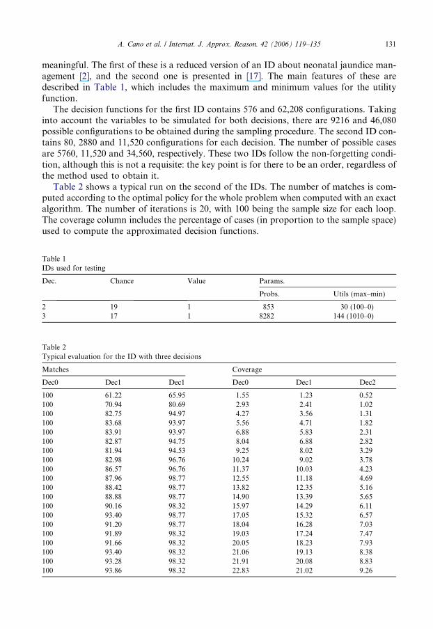
meaningful. The first of these is a reduced version of an ID about neonatal jaundice man-agement [2], and the second one is presented in [17]. The main features of these aredescribed in Table 1, which includes the maximum and minimum values for the utilityfunction.

The decision functions for the first ID contains 576 and 62,208 configurations. Takinginto account the variables to be simulated for both decisions, there are 9216 and 46,080possible configurations to be obtained during the sampling procedure. The second ID con-tains 80, 2880 and 11,520 configurations for each decision. The number of possible casesare 5760, 11,520 and 34,560, respectively. These two IDs follow the non-forgetting condi-tion, although this is not a requisite: the key point is for there to be an order, regardless ofthe method used to obtain it.

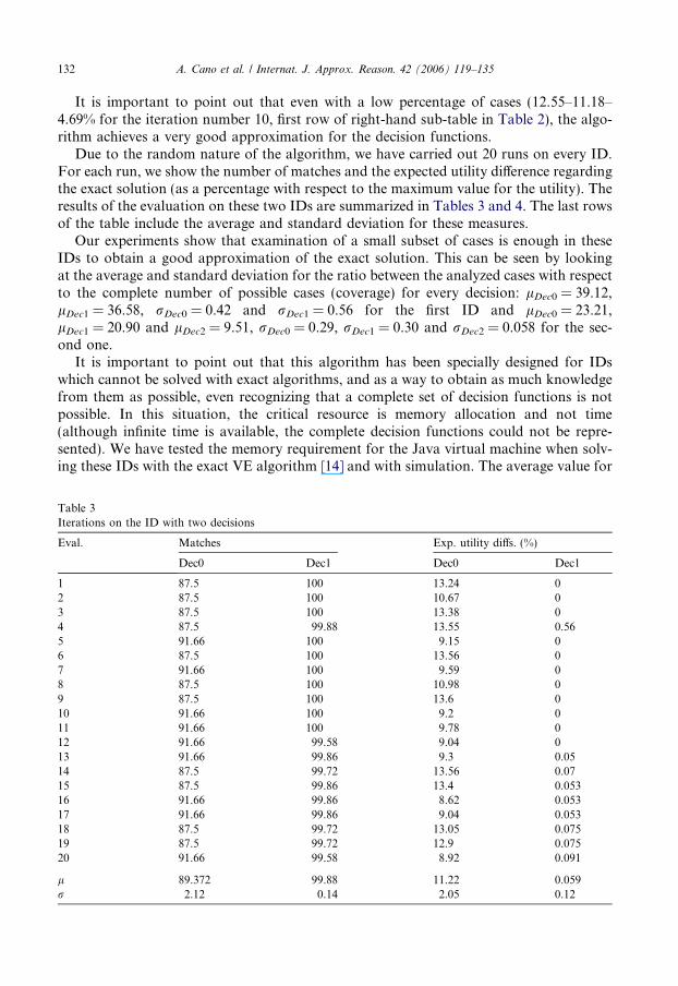
Table 2 shows a typical run on the second of the IDs. The number of matches is com-puted according to the optimal policy for the whole problem when computed with an exactalgorithm. The number of iterations is 20, with 100 being the sample size for each loop.The coverage column includes the percentage of cases (in proportion to the sample space)used to compute the approximated decision functions.

Table 1IDs used for testing

Dec. Chance Value Params.

Probs. Utils (max–min)

2 19 1 853 30 (100–0)3 17 1 8282 144 (1010–0)

Table 2Typical evaluation for the ID with three decisions

Matches Coverage

Dec0 Dec1 Dec1 Dec0 Dec1 Dec2

100 61.22 65.95 1.55 1.23 0.52100 70.94 80.69 2.93 2.41 1.02100 82.75 94.97 4.27 3.56 1.31100 83.68 93.97 5.56 4.71 1.82100 83.91 93.97 6.88 5.83 2.31100 82.87 94.75 8.04 6.88 2.82100 81.94 94.53 9.25 8.02 3.29100 82.98 96.76 10.24 9.02 3.78100 86.57 96.76 11.37 10.03 4.23100 87.96 98.77 12.55 11.18 4.69100 88.42 98.77 13.82 12.35 5.16100 88.88 98.77 14.90 13.39 5.65100 90.16 98.32 15.97 14.29 6.11100 93.40 98.77 17.05 15.32 6.57100 91.20 98.77 18.04 16.28 7.03100 91.89 98.32 19.03 17.24 7.47100 91.66 98.32 20.05 18.23 7.93100 93.40 98.32 21.06 19.13 8.38100 93.28 98.32 21.91 20.08 8.83100 93.86 98.32 22.83 21.02 9.26

132 A. Cano et al. / Internat. J. Approx. Reason. 42 (2006) 119–135

It is important to point out that even with a low percentage of cases (12.55–11.18–4.69% for the iteration number 10, first row of right-hand sub-table in Table 2), the algo-rithm achieves a very good approximation for the decision functions.

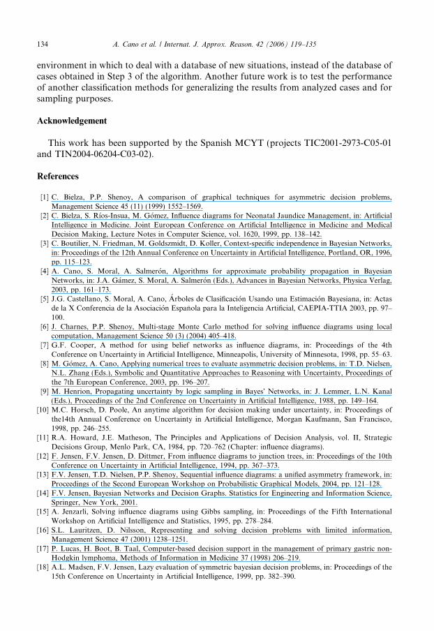
Due to the random nature of the algorithm, we have carried out 20 runs on every ID.For each run, we show the number of matches and the expected utility difference regardingthe exact solution (as a percentage with respect to the maximum value for the utility). Theresults of the evaluation on these two IDs are summarized in Tables 3 and 4. The last rowsof the table include the average and standard deviation for these measures.

Our experiments show that examination of a small subset of cases is enough in theseIDs to obtain a good approximation of the exact solution. This can be seen by lookingat the average and standard deviation for the ratio between the analyzed cases with respectto the complete number of possible cases (coverage) for every decision: lDec0 = 39.12,lDec1 = 36.58, rDec0 = 0.42 and rDec1 = 0.56 for the first ID and lDec0 = 23.21,lDec1 = 20.90 and lDec2 = 9.51, rDec0 = 0.29, rDec1 = 0.30 and rDec2 = 0.058 for the sec-ond one.

It is important to point out that this algorithm has been specially designed for IDswhich cannot be solved with exact algorithms, and as a way to obtain as much knowledgefrom them as possible, even recognizing that a complete set of decision functions is notpossible. In this situation, the critical resource is memory allocation and not time(although infinite time is available, the complete decision functions could not be repre-sented). We have tested the memory requirement for the Java virtual machine when solv-ing these IDs with the exact VE algorithm [14] and with simulation. The average value for

Table 3Iterations on the ID with two decisions

Eval. Matches Exp. utility diffs. (%)

Dec0 Dec1 Dec0 Dec1

1 87.5 100 13.24 02 87.5 100 10.67 03 87.5 100 13.38 04 87.5 99.88 13.55 0.565 91.66 100 9.15 06 87.5 100 13.56 07 91.66 100 9.59 08 87.5 100 10.98 09 87.5 100 13.6 010 91.66 100 9.2 011 91.66 100 9.78 012 91.66 99.58 9.04 013 91.66 99.86 9.3 0.0514 87.5 99.72 13.56 0.0715 87.5 99.86 13.4 0.05316 91.66 99.86 8.62 0.05317 91.66 99.86 9.04 0.05318 87.5 99.72 13.05 0.07519 87.5 99.72 12.9 0.07520 91.66 99.58 8.92 0.091

l 89.372 99.88 11.22 0.059r 2.12 0.14 2.05 0.12

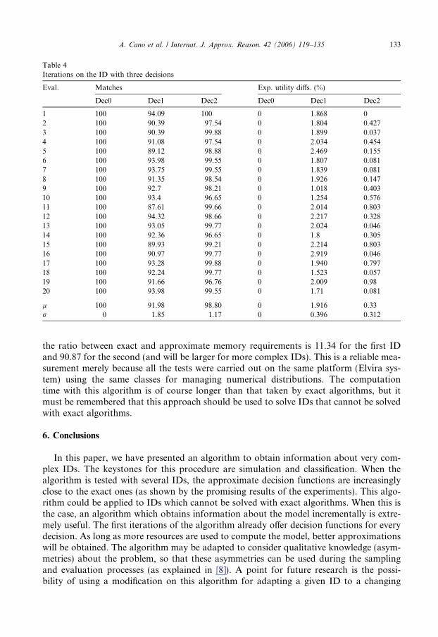
Table 4Iterations on the ID with three decisions

Eval. Matches Exp. utility diffs. (%)

Dec0 Dec1 Dec2 Dec0 Dec1 Dec2

1 100 94.09 100 0 1.868 02 100 90.39 97.54 0 1.804 0.4273 100 90.39 99.88 0 1.899 0.0374 100 91.08 97.54 0 2.034 0.4545 100 89.12 98.88 0 2.469 0.1556 100 93.98 99.55 0 1.807 0.0817 100 93.75 99.55 0 1.839 0.0818 100 91.35 98.54 0 1.926 0.1479 100 92.7 98.21 0 1.018 0.40310 100 93.4 96.65 0 1.254 0.57611 100 87.61 99.66 0 2.014 0.80312 100 94.32 98.66 0 2.217 0.32813 100 93.05 99.77 0 2.024 0.04614 100 92.36 96.65 0 1.8 0.30515 100 89.93 99.21 0 2.214 0.80316 100 90.97 99.77 0 2.919 0.04617 100 93.28 99.88 0 1.940 0.79718 100 92.24 99.77 0 1.523 0.05719 100 91.66 96.76 0 2.009 0.9820 100 93.98 99.55 0 1.71 0.081

l 100 91.98 98.80 0 1.916 0.33r 0 1.85 1.17 0 0.396 0.312

A. Cano et al. / Internat. J. Approx. Reason. 42 (2006) 119–135 133

the ratio between exact and approximate memory requirements is 11.34 for the first IDand 90.87 for the second (and will be larger for more complex IDs). This is a reliable mea-surement merely because all the tests were carried out on the same platform (Elvira sys-tem) using the same classes for managing numerical distributions. The computationtime with this algorithm is of course longer than that taken by exact algorithms, but itmust be remembered that this approach should be used to solve IDs that cannot be solvedwith exact algorithms.

6. Conclusions

In this paper, we have presented an algorithm to obtain information about very com-plex IDs. The keystones for this procedure are simulation and classification. When thealgorithm is tested with several IDs, the approximate decision functions are increasinglyclose to the exact ones (as shown by the promising results of the experiments). This algo-rithm could be applied to IDs which cannot be solved with exact algorithms. When this isthe case, an algorithm which obtains information about the model incrementally is extre-mely useful. The first iterations of the algorithm already offer decision functions for everydecision. As long as more resources are used to compute the model, better approximationswill be obtained. The algorithm may be adapted to consider qualitative knowledge (asym-metries) about the problem, so that these asymmetries can be used during the samplingand evaluation processes (as explained in [8]). A point for future research is the possi-bility of using a modification on this algorithm for adapting a given ID to a changing

134 A. Cano et al. / Internat. J. Approx. Reason. 42 (2006) 119–135

environment in which to deal with a database of new situations, instead of the database ofcases obtained in Step 3 of the algorithm. Another future work is to test the performanceof another classification methods for generalizing the results from analyzed cases and forsampling purposes.

Acknowledgement

This work has been supported by the Spanish MCYT (projects TIC2001-2973-C05-01and TIN2004-06204-C03-02).

References

[1] C. Bielza, P.P. Shenoy, A comparison of graphical techniques for asymmetric decision problems,Management Science 45 (11) (1999) 1552–1569.

[2] C. Bielza, S. Rıos-Insua, M. Gomez, Influence diagrams for Neonatal Jaundice Management, in: ArtificialIntelligence in Medicine. Joint European Conference on Artificial Intelligence in Medicine and MedicalDecision Making, Lecture Notes in Computer Science, vol. 1620, 1999, pp. 138–142.

[3] C. Boutilier, N. Friedman, M. Goldszmidt, D. Koller, Context-specific independence in Bayesian Networks,in: Proceedings of the 12th Annual Conference on Uncertainty in Artificial Intelligence, Portland, OR, 1996,pp. 115–123.

[4] A. Cano, S. Moral, A. Salmeron, Algorithms for approximate probability propagation in BayesianNetworks, in: J.A. Gamez, S. Moral, A. Salmeron (Eds.), Advances in Bayesian Networks, Physica Verlag,2003, pp. 161–173.

[5] J.G. Castellano, S. Moral, A. Cano, Arboles de Clasificacion Usando una Estimacion Bayesiana, in: Actasde la X Conferencia de la Asociacion Espanola para la Inteligencia Artificial, CAEPIA-TTIA 2003, pp. 97–100.

[6] J. Charnes, P.P. Shenoy, Multi-stage Monte Carlo method for solving influence diagrams using localcomputation, Management Science 50 (3) (2004) 405–418.

[7] G.F. Cooper, A method for using belief networks as influence diagrams, in: Proceedings of the 4thConference on Uncertainty in Artificial Intelligence, Minneapolis, University of Minnesota, 1998, pp. 55–63.

[8] M. Gomez, A. Cano, Applying numerical trees to evaluate asymmetric decision problems, in: T.D. Nielsen,N.L. Zhang (Eds.), Symbolic and Quantitative Approaches to Reasoning with Uncertainty, Proceedings ofthe 7th European Conference, 2003, pp. 196–207.

[9] M. Henrion, Propagating uncertainty by logic sampling in Bayes� Networks, in: J. Lemmer, L.N. Kanal(Eds.), Proceedings of the 2nd Conference on Uncertainty in Artificial Intelligence, 1988, pp. 149–164.

[10] M.C. Horsch, D. Poole, An anytime algorithm for decision making under uncertainty, in: Proceedings ofthe14th Annual Conference on Uncertainty in Artificial Intelligence, Morgan Kaufmann, San Francisco,1998, pp. 246–255.

[11] R.A. Howard, J.E. Matheson, The Principles and Applications of Decision Analysis, vol. II, StrategicDecisions Group, Menlo Park, CA, 1984, pp. 720–762 (Chapter: influence diagrams).

[12] F. Jensen, F.V. Jensen, D. Dittmer, From influence diagrams to junction trees, in: Proceedings of the 10thConference on Uncertainty in Artificial Intelligence, 1994, pp. 367–373.

[13] F.V. Jensen, T.D. Nielsen, P.P. Shenoy, Sequential influence diagrams: a unified asymmetry framework, in:Proceedings of the Second European Workshop on Probabilistic Graphical Models, 2004, pp. 121–128.

[14] F.V. Jensen, Bayesian Networks and Decision Graphs. Statistics for Engineering and Information Science,Springer, New York, 2001.

[15] A. Jenzarli, Solving influence diagrams using Gibbs sampling, in: Proceedings of the Fifth InternationalWorkshop on Artificial Intelligence and Statistics, 1995, pp. 278–284.

[16] S.L. Lauritzen, D. Nilsson, Representing and solving decision problems with limited information,Management Science 47 (2001) 1238–1251.

[17] P. Lucas, H. Boot, B. Taal, Computer-based decision support in the management of primary gastric non-Hodgkin lymphoma, Methods of Information in Medicine 37 (1998) 206–219.

[18] A.L. Madsen, F.V. Jensen, Lazy evaluation of symmetric bayesian decision problems, in: Proceedings of the15th Conference on Uncertainty in Artificial Intelligence, 1999, pp. 382–390.

A. Cano et al. / Internat. J. Approx. Reason. 42 (2006) 119–135 135

[19] P.P. Ndilikilikesha, Potential influence diagrams, International Journal of Approximate Reasoning 11 (1994)251–285.

[20] T.D. Nielsen, F.V. Jensen, Well-defined decision scenarios, in: K.B. Laskey, H. Prade (Eds.), Uncertainty inArtificial Intelligence, Proceedings of the 15th Conference, Morgan Kaufmann, Los Altos, CA, 1999, pp.502–511.

[21] T.D. Nielsen, F.V. Jensen, Representing and solving asymmetric Bayesian decision problems, in: C.Boutilier, M. Goldszmidt (Eds.), Proceedings of the 16th Conference on Uncertainty in ArtificialIntelligence, 2000, pp. 416–425.

[22] D. Nilsson, F.V. Jensen, Springer Lecture Notes in Artificial Intelligence: Information, Uncertainty, Fusion,2000, pp. 161–171 (Chapter: probabilities of future decisions).

[23] J.R. Quinlan, Induction of decision trees, Machine Learning 1 (1986) 81–106.[24] R.D. Shachter, Efficient value of information computation, in: Proceedings of the 15th Conference on

Uncertainty and Artificial Intelligence, 1999, pp. 594–601.[25] R.D. Shachter, P.P Ndilikilikesha, Using potential influence diagrams for probabilistic inference and

decision making, in: Proceedings of the 9th Conference on Uncertainty and Artificial Intelligence, 1993, pp.383–390.

[26] R.D. Shachter, M.A. Peot, Decision making using probabilistic inference methods, in: Proceedings of the 8thConference on Uncertainty in Artificial Intelligence, San Jose, 1992, pp. 276–283.

[27] R.D. Shachter, Evaluating influence diagrams, Operations Research 34 (1986) 871–882.[28] P.P. Shenoy, Valuation-based systems for Bayesian decision analysis, Operations Research 40 (3) (1992) 463–

484.[29] P.P. Shenoy, A new method for representing and solving Bayesian decision problems, in: Artificial

Intelligence Frontiers in Statistics: AI and Statistics, Chapman & Hall, London, 1993, pp. 119–138.[30] J.E. Smith, S. Holtzman, J.E. Matheson, Structuring conditional relationships in influence diagrams,

Operations Research 41 (2) (1993) 280–297.[31] J.A. Tatman, R.D. Shachter, Dynamic programming and influence diagrams, IEEE Transactions on

Systems, Man and Cybernetics 20 (2) (1990) 365–379.[32] N.L. Zhang, Probabilistic inference in influence diagrams, in: Proceedings of the 14th Annual Conference on

Uncertainty in Artificial Intelligence, Morgan Kaufmann, San Francisco, 1998, pp. 514–522.