A Formal Model of Molecular Codes with Respect to Chemical Reaction Networks Dissertation zur Erlangung des akademischen Grades doctor rerum naturalium (Dr. rer. nat.) vorgelegt dem Rat der Fakult¨ at f¨ ur Mathematik und Informatik der Friedrich-Schiller-Universit¨at Jena von Diplom-Bioinformatiker Dennis G¨ orlich geboren am 02. Juni 1983 in Hagen

Welcome message from author
This document is posted to help you gain knowledge. Please leave a comment to let me know what you think about it! Share it to your friends and learn new things together.
Transcript
A Formal Model of MolecularCodes with Respect to Chemical
Reaction Networks
Dissertation
zur Erlangung des akademischen Grades
doctor rerum naturalium (Dr. rer. nat.)
vorgelegt dem
Rat der Fakultat fur Mathematik und Informatik
der
Friedrich-Schiller-Universitat Jena
von
Diplom-Bioinformatiker Dennis Gorlich
geboren am
02. Juni 1983 in Hagen

Gutachter1. PD Dr. Peter Dittrich (Friedrich-Schiller-Universitat Jena)2. PD Dr. Stefan Artmann (Friedrich-Schiller-Universitat Jena)3. Prof. Dr. Marcello Barbieri (Universita di Ferrara)
Tag der offentlichen Verteidigung: 19.04.2013
Abstract
The present thesis introduces a theory of molecular codes with respect to chemicalreaction networks. Codes, in general, are mappings between sets of entities. Encodingis very well known in many disciplines, like language, where concepts are said to beencoded in words or spoken language, and computer science where, e.g. commands haveto be encoded into binary digits for execution, or optimal codes for data compressinghave to be developed. In biology the notion of codes has been largely introduced togetherwith the discovery of the gene translation mechanisms, i.e. the genetic code. Recentdevelopments in molecular and cellular biology postulate other molecular codes besidethe genetic code, e.g. the histone code or the sugar code. In the literature these codesare described in detail in their biochemical mechanisms, but the usage of the term”code” is ambiguous. Often ”code” denotes only the codewords, e.g. combinationsof covalent histone modifications, but neglects the mapping between codewords andtheir ”meanings”. It is also not yet clear which biological relevant entities (processes,molecular species, system states) are encoded by these novel codes. One reason for theunclear usage of the code concept is the lack of an objective definition of a ”molecularcode” applicable to biological systems. To enable molecular biology to properly analysemolecular codes a formal, objective and testable definition of code is necessary. In thisthesis I will present a formal concept of molecular codes as mappings between sets ofmolecular species that are elements of a chemical reaction network, i.e. a model of a(bio-)chemical system.An important property of a code is its contingency, i.e. the relations between codewordsand their ”meanings” could, in principle, be different. This should also hold for molec-ular codes to distinguish them from fixed mappings and to enable evolution to act oncodes. Due to the contingency condition codes always occur as collection of (potential)mappings. These differ in their actual relations, but map the same sets of molecularspecies. The general definition of molecular codes as contingent molecular mappingsis specialised by analysing binary molecular codes, i.e. codes between sets of only twomolecular species. Furthermore, the definition of codes allows to analyse the propertiesof molecular codes, especially the relations between codes. I will analyse code nestingand code linkage as two forms of code relations. Both concept allow to describe cells assystems of codes.Based on the definition of molecular codes it is possible to develop algorithms to iden-tify codes in chemical reaction networks. I propose two different algorithms based ondifferent structural network properties, i.e. on closed sets and paths, respectively. Bothalgorithms follow a brute force strategy and are computational not feasible for largenetworks. For the path algorithm I propose two heuristic variants, i.e. (1) using thek-shortest paths (instead of all paths), and (2) applying a Monte-Carlo-type subnetworksampling with subsequent code analysis. The two heuristics do not guarantee to identifyall codes, but generate an estimate on the number of codes. This approach is suited forlarge scale networks, as demonstrated for the metabolic network of cells and the humansignal transduction network.The algorithms are applied to a number of different reaction networks modelling com-bustion chemistries, a planetary photo chemistry, the gene translation system, the generegulatory network, signalling by phosphorylation cascades, and two large scale biologi-cal networks obtained from databases. The analysis of these networks shows that abioticnetworks do not have the ability to realize codes, while the biochemical systems do havethe ability to implement molecular codes. The example of a phosphorylation cascade
network model shows the restriction to the structural approach of code identification,since here codes can only be implemented when the species’ concentration is considered.Random networks are analysed as a null model of molecular codes. A statistical modelis fitted that describes the number of molecular codes dependent on network size andnetwork density. The analysis also shows that there exist an optimal interval for codesfor a fixed network size. Very sparse networks and very dense networks do not allowfor molecular coding. The optimal interval gives the network densities that allow for alarge number of codes, assuming completely random processes of network generation.The analysis of an artificial chemistry shows that also a dense network can have codes.A randomisation study of this network results in a decrease in the number of codes,i.e. the network converges towards the null model. Similarly, we can assume that thenumber of codes could increase under random variation if the network is in the optimalinterval.From a theoretical point of view the ability to implement codes can be interpreted assemantic capacity. By identifying potential molecular codes a measure for the semanticcapacity of (bio-)chemical systems is provided. Based on this notion hypotheses can beformulated with respect to the semantic capacity of biological systems, e.g. cells evolvetowards higher semantic capacity, by employing subnetworks (subchemistries) that allowfor coding. The results of this thesis will not answer this question completely, but givefirst results.In the thesis I will also discuss how the static, semantic aspect of molecular codes canbe (and has to be) supplemented by the pragmatic level, e.g. by including kinetics andprobabilities. The inclusion of dynamics also allows to identify codes between wholesystem states.
Zusammenfassung
In der vorliegenden Dissertation fuhre ich ein formales Konzept fur molekularer Kodesin chemischen Reaktionsnetzwerken ein. Kodes sind Abbildungen zwischen Mengen vonObjekten. Kodierung ist ein verbreitetes Konzept. In der Linguistik wird der Zusam-menhang zwischen Wortern und den bezeichneten Objekten als Kodierung aufgefasst. Inder Informatik werden Instruktionen in Bitstrings kodiert werden, bzw. optimale Kodesfur Dateikomprimierung entwickelt. In der Biologie wurde das Kodekonzept zusammenmit der Entdeckung der Mechanismen der Gentranslation eingefuhrt, der genetischeKode. Die weitere Forschung in der Zell- und Molekularbiologie postuliert die Existenzweiterer Kodes in der Zelle neben dem genetischen Kode. Der Histone- und der Zuck-erkode sind hier Beispiele. Diese neuartigen Kodes wurden bisher sehr detailiert in ihrenbiochemischen Mechanismen beschrieben, aber nutzen Unterschiedliche Definitionen desKodebegriffs. Oft wird der Begriff ”Kode” zur Bezeichnung der Kodeworter, zumBeispiel die Kombination verschiedener kovalenter Histonemodifikationen, verwendet,wahrend die Bedeutung im Sinne einer Abbildung vernachlassigt wird. Dabei ist es auchnicht klar zwischen welchen Mengen (Prozesse, molekulare Spezies, Systemzustande )abgebildet wird. Ein Grund fur die unklare Verwendung des Kodebegriffs ist das Fehleneiner objektiven Definition, die es erlaubt molekulare Kodes in biologischen Systemenzu erkennen. Eine formale, objektive und prufbare Definition ist daher notwendig. DasKodekonzept, das hier vorgestellt werden soll, basiert auf Modellen chemischer Systemein Form von chemischen Reaktionsnetzwerken.Ein wichtiger Aspekt von Kodes im allgemeinen ist Kontingenz. Eine kontingenteAbbildung erlaubt es die Kodeworter und deren Bedeutungen willkurlich zuzuordnen,d.h. eine beobachtete Abbildung konnte prinzipiell auch in anderer Auspragung vor-liegen. Dies soll auch fur molekulare Kodes gelten. Molekulare Kodes unterscheidensich dadurch von feste Abbildungen und konnen als Ziel eines evolutionaren Selektions-drucks fungieren. Die Kontingenzbedingung bewirkt, dass Kodes immer als Menge vieler(potentieller) Kodes auftreten. Diese Kodes unterscheiden sich in ihren Beziehungen,aber bilden zwischen den selben Mengen ab. Ein Spezialfall der allgemeinen Defini-tion molekularer Kodes stellt die Analyse binarer molekularer Kodes dar. Dies sindmolekulare Kodes, die zwischen binaren Mengen abbilden. Die Definition molekularerKodes erlaubt außerdem die Analyse bestimmter Kodeeigenschaften, zum Beispiel Rela-tionen zwischen Kodes. Ich habe in diesem Zusammenhang verschachtelte Kodes (codenesting) und zwei Formen der Kodeverknupfung (code linkage) untersucht. Die Ver-wendung dieser Eigenschaften ermoglicht es die Zelle als System molekularer Kodes zubeschreiben.Basierend auf der Definition ist es moglich Algorithmen zur Kodeidentifikation in chemis-chen Reaktionsnetzwerken anzugeben. Ich stelle zwei Algorithmen vor, die unterschiedlicheNetzwerkeigenschaften ausnutzen, zum Einen geschlossene Mengen und zum Anderendie Pfade durch das Netzwerk. Beide Algorithmen folgen einer brute-force Strategieund sind fur große Netzwerke sehr rechenintensiv. Fur den Pfadalgorithmus stelle ichzwei Heuristiken vor. Die erste Heuristik verwendet die K kurzesten Pfade, wahrenddie zweite Heuristik zusatzlich in einem Monte-Carlo Ansatz Teilnetzwerke ermittelt,die anschließend mit dem Kodealgorithmus analysiert werden. Die entwickelten Algo-rithmen werden auf verschiedene Netzwerkmodelle angewandt: Verbrennungschemien,eine planetare Photochemie, das Gentranslationssystem, genregulatorische Netzwerke,Signalweiterleitung durch Phosporylierungskaskaden und zwei große biologische Netzw-erke (Metabolism und Signaltransduktion) die aus Netzwerkdatenbanken stammen. Die
Analyse dieser Netzwerke zeigt dass abiotische Netze keine Kodes besitzen, wahrend diebiologischen Netzwerkmodelle sehr viele molekulare Kodes implementieren konnen. DasBeispiel der Phosphorilierungkaskaden zeigt aber auch die Grenzen dieses Ansatzes, dahier Konzentrationen zur Kodeidentifizierung hinzugezogen werden mussen. ZufalligeReaktionsnetzwerke konnen als Nullmodell fur molekularer Kodes dienen, indem einstatistisches Modell angelernt wird, das die Anzahl molekularer Kodes in Abhangigkeitder Netzwerkgroße und Dichte beschreibt. Die Analyse der Daten zeigt auch, dasses ein optimales Interval (bezogen auf die Netzwerkdichte) fur molekulare Kodes gibt.Sehr dunne und sehr dichte Netzwerke erlauben demnach keine Realisierung moleku-larer Kodes. Das optimale Interval gibt an welche Netzwerkdichten die Realisierungvieler molekularer Codes erlauben, unter der Anahme einer komplett zufalligen Net-zwerkgenerierung. Die Analyse einer kunstlichen Chemie zeigt, dass auch dichte Net-zwerke Kodes enthalten konnen. Die Randomisierung dieses Netzwerks fuhrt zu einerVerringerung der Kodierungskapazitat, das Netztwerk konvergiert gegen das Nullmod-ell. Daran angelehnt kann die Hypothese aufgestellt werden, dass die Anzahl moleku-larer Kodes ansteigen kann, wenn das Netzwerk sich im optimalen Interval befindet.Die Fahigkeit eines Systems molekulare Kodes zu implementieren kann als semantis-che Kapazitat aufgefasst werden, da ein Kode Zeichen und Bedeutungen miteinanderverknupft. Die Identifizierung molekularer Kodes liefert daher ein Maß fur die seman-tische Kapazitat eines Systems. Darauf basierend konnen Hypothesen in Bezug aufdie semantische Kapazitat biologischer Systeme formuliert werden, zum Beispiel, dassZellen im Laufe ihrer Evolution mehr Subsysteme hoher semantischer Kapazitat ver-wenden. Die vorliegende Arbeit wird diese Frage nicht abschließend beantworten, son-dern liefert erste Resultate. Zum Ende der Arbeit diskutiere ich die Notwendigkeitden hier vorgestellten statischen Ansatz durch pragmatische Aspekte, d.h. Dynamik,Kinetiken und Wahrscheinlichkeiten, zu erweitern. Die Erweiterung um dynamische As-pekte ermoglicht zum Beispiel die Identifizierung von Kodes zwischen Systemzustanden.
Acknowledgements
First of all I want to thank Peter Dittrich for giving me the opportunity to do a PhD inhis group and for finding time to discuss new ideas and to give support and advice. Ialso want to thank Stefan Artmann for all the discussions and input, especially, at thebeginning of my project. Stefan Heinemann, as member of my JSMC thesis committee,for finding time for our meetings and for giving valuable input. My thanks goes tothe members of the Bio Systems Analysis Group for providing an open ear for newideas, for interesting discussions, for giving support and for almost always sharing theirsweets. I want to thank Konstantin Riege who helped at the implementation of therandom subnetwork sampling algorithm. I also want to thank Conny Musse and KathrinSchowtka for helping me through the university’s bureaucracy. The support of thefaculty’s computer center staff was always appreciated to overcome minor and major ITissues.I had the luck to be supported by a stipend of the excellence initiative graduate school”Jena School for Microbial Communication (JSMC)”, which allowed many freedomsthat would not be possible with other forms of funding. As JSMC fellow representativeI want to thank the teams of representatives I had the luck to work in: The first teamof representatives Nadine and Anne, the follow-up team Markus and Cris and the newteam Sarahi, Markus and Martin, and Frank our long term JSMC representative. I alsowant to thank the organising teams of our conference ”International Student Conferenceon Microbial Communication (MICOM)” which we started in 2010. Organising thisconference was a lot of work (especially the first time), but also was lot of fun andyielded lots of experiences. Special thanks go to Carsten Thoms and Ulrike Schleierfrom the JSMC management. Both did and do an extraordinary job, and without theirwork JSMC would not be as successful and well organised as it is.Finally, I want to thank my family for their ongoing support. My parents and parents-in-law for giving all kinds of support. My wonderful son Linus for being just as he isand with whom I will start many new adventures in future. My last and deepest thanksgo to my wonderful wife Stephanie who always encourages me to go on and focus onthe important things.
7

Contents
1 Introduction 111.1 Biological information processing . . . . . . . . . . . . . . . . . . . . . . 111.2 Related formal concepts . . . . . . . . . . . . . . . . . . . . . . . . . . . 131.3 Structure of the thesis . . . . . . . . . . . . . . . . . . . . . . . . . . . . 15
2 The notion of ”Code” in biological research 172.1 Gene translation – The genetic code . . . . . . . . . . . . . . . . . . . . . 172.2 Covalent histone modifications - The histone code . . . . . . . . . . . . . 182.3 Glycan recognition – The sugar code . . . . . . . . . . . . . . . . . . . . 192.4 Summary . . . . . . . . . . . . . . . . . . . . . . . . . . . . . . . . . . . 21
3 A formalisation of molecular codes 233.1 Formalisation of molecular codes in chemical reaction networks . . . . . . 233.2 Binary molecular codes . . . . . . . . . . . . . . . . . . . . . . . . . . . . 263.3 Semantic capacity . . . . . . . . . . . . . . . . . . . . . . . . . . . . . . . 283.4 Relations among codes . . . . . . . . . . . . . . . . . . . . . . . . . . . . 29
3.4.1 Code pair equality . . . . . . . . . . . . . . . . . . . . . . . . . . 293.4.2 Nested molecular codes . . . . . . . . . . . . . . . . . . . . . . . . 303.4.3 Code linkages . . . . . . . . . . . . . . . . . . . . . . . . . . . . . 33
4 Algorithmic code identification 374.1 Network representation . . . . . . . . . . . . . . . . . . . . . . . . . . . . 374.2 Obtaining suitable reaction networks . . . . . . . . . . . . . . . . . . . . 374.3 Closure-based algorithm . . . . . . . . . . . . . . . . . . . . . . . . . . . 384.4 Pathway-based algorithm . . . . . . . . . . . . . . . . . . . . . . . . . . . 394.5 Implementation and runtime evaluation . . . . . . . . . . . . . . . . . . . 424.6 A random sampling algorithm for BMC identification . . . . . . . . . . . 434.7 Code completion . . . . . . . . . . . . . . . . . . . . . . . . . . . . . . . 46
5 Results of the algorithmic code analysis of various systems 495.1 Random networks . . . . . . . . . . . . . . . . . . . . . . . . . . . . . . . 495.2 Combustion chemistries . . . . . . . . . . . . . . . . . . . . . . . . . . . 585.3 The artificial chemistry NTOP . . . . . . . . . . . . . . . . . . . . . . . . 595.4 Photochemistry of Mars . . . . . . . . . . . . . . . . . . . . . . . . . . . 605.5 The genetic code . . . . . . . . . . . . . . . . . . . . . . . . . . . . . . . 615.6 Gene regulatory networks . . . . . . . . . . . . . . . . . . . . . . . . . . 665.7 Protein assembly . . . . . . . . . . . . . . . . . . . . . . . . . . . . . . . 725.8 Signalling by phosphorylation cascades. . . . . . . . . . . . . . . . . . . . 725.9 Analysis of large scale biological networks . . . . . . . . . . . . . . . . . 76
9
5.9.1 Metabolism . . . . . . . . . . . . . . . . . . . . . . . . . . . . . . 765.9.2 Cellular signal transduction . . . . . . . . . . . . . . . . . . . . . 76
5.10 Summary . . . . . . . . . . . . . . . . . . . . . . . . . . . . . . . . . . . 81
6 Towards pragmatics 856.1 Code validation . . . . . . . . . . . . . . . . . . . . . . . . . . . . . . . . 856.2 Code determination . . . . . . . . . . . . . . . . . . . . . . . . . . . . . . 876.3 Codes between system states . . . . . . . . . . . . . . . . . . . . . . . . . 88
7 Discussion and Outlook 91
References 103
A Helper methods 111A.1 Random network generation . . . . . . . . . . . . . . . . . . . . . . . . . 111A.2 Methods for the closure-based algorithm . . . . . . . . . . . . . . . . . . 111A.3 Methods for the pathway-based algorithms . . . . . . . . . . . . . . . . . 113
B Proof of Lemma 3.2.1 117
C Potential codes in signal transduction 119
D Potential codes in metabolism 127
E Networks 131E 1 Example networks . . . . . . . . . . . . . . . . . . . . . . . . . . . . . . . 132
E 1.1 BMC 1 . . . . . . . . . . . . . . . . . . . . . . . . . . . . . . . . . 132E 1.2 BMC 2 . . . . . . . . . . . . . . . . . . . . . . . . . . . . . . . . . 132E 1.3 Extended BMC . . . . . . . . . . . . . . . . . . . . . . . . . . . . 132
E 2 Combustion chemistries . . . . . . . . . . . . . . . . . . . . . . . . . . . 132E 2.1 Dimethyl ether . . . . . . . . . . . . . . . . . . . . . . . . . . . . 132E 2.2 Ethanol . . . . . . . . . . . . . . . . . . . . . . . . . . . . . . . . 138E 2.3 Hydrogen . . . . . . . . . . . . . . . . . . . . . . . . . . . . . . . 143E 2.4 Methane . . . . . . . . . . . . . . . . . . . . . . . . . . . . . . . . 144
E 3 Artificial chemistry NTOP . . . . . . . . . . . . . . . . . . . . . . . . . . 146E 4 Gene translation . . . . . . . . . . . . . . . . . . . . . . . . . . . . . . . 148
E 4.1 NCBI Merge . . . . . . . . . . . . . . . . . . . . . . . . . . . . . . 148E 4.2 Completed GC w/o synthetases (excerpt) . . . . . . . . . . . . . . 151E 4.3 Complete GC with synthetases (excerpt) . . . . . . . . . . . . . . 151
E 5 Gene regulatory networks . . . . . . . . . . . . . . . . . . . . . . . . . . 152E 5.1 GC-GRN network . . . . . . . . . . . . . . . . . . . . . . . . . . . 152E 5.2 Extended GC-GRN network . . . . . . . . . . . . . . . . . . . . . 152
E 6 Phosphorylation cascades . . . . . . . . . . . . . . . . . . . . . . . . . . . 152E 6.1 Simple phosphorylation model . . . . . . . . . . . . . . . . . . . . 152E 6.2 Extended phosphorylation model . . . . . . . . . . . . . . . . . . 153
E 7 Protein assembly . . . . . . . . . . . . . . . . . . . . . . . . . . . . . . . 153E 7.1 Two steps, without dissociation . . . . . . . . . . . . . . . . . . . 153E 7.2 Two steps, with dissociation . . . . . . . . . . . . . . . . . . . . . 153
E 8 Photochemistry of Mars . . . . . . . . . . . . . . . . . . . . . . . . . . . 154E 9 Signal transduction and metabolic network . . . . . . . . . . . . . . . . . 155
10
Chapter 1
Introduction
1.1 Biological information processing
Research of the last decades showed that cells communicate and process information [1].This is not only true for human cells, where, for example, the hormone system is wellknown, but also for all other eukaryotic and prokaryotic species. While communicationrefers to an interaction between individual cells, information processing is a more generalconcept. The genetic system, implemented in every cell, maintains the blueprint for thecell’s components, e.g. proteins. This stored information is utilised by the processesusually referred to as transcription and translation, in the case of proteins. Beside thegenetic system cells maintain complex signal transduction networks that enables themto integrate information about their environment, internal state and incoming signals.This information is mainly used to regulate the cell’s behaviour, i.e. to change theinternal state.
The understanding of biological information processing is not only relevant as basicresearch, but can have direct practical applications, for example, to identify targets inthe treatment of microbial infections [2]. From a theoretical point of view it is also ofinterest if different subsystems (biochemical systems) of cells are better suited to beused for information processing.
Syntax, semantics and pragmatics For theoretical analysis of biological informa-tion Shannon’s theory of communication [3] has been applied successfully in variousdomains, like gene regulatory networks [4], bacterial quorum sensing [5], or signalling inmolecular systems [6, 1]. The mathematical theory of communication focusses on un-certainty of events and intentionally neglects semantic aspects of information, because”they are irrelevant for the engineering problem” (Shannon [3], p. 1). In order to obtaina full understanding of biological information, studying semantic as well as pragmaticaspects would be important, if not necessary [7, 8].
The terms syntax, semantics and pragmatics 1 are concepts borrowed from the fieldsof language and semiotics. The transfer from these fields of study to the life sciencesneeds to be justified. Whether the linguistic terms used in biology are ill-posed orvaluable concepts is discussed [10, 11]. These concepts have explanatory power in bio-logical systems as discussed, for example, in [12]. The analogy between communicationprocesses in language and semiotics, and molecular communication (where signals are
1For a detailed introduction to syntax, semantics, and pragmatics as semiotic concepts see forexample [9].
11
1.1. Biological information processing
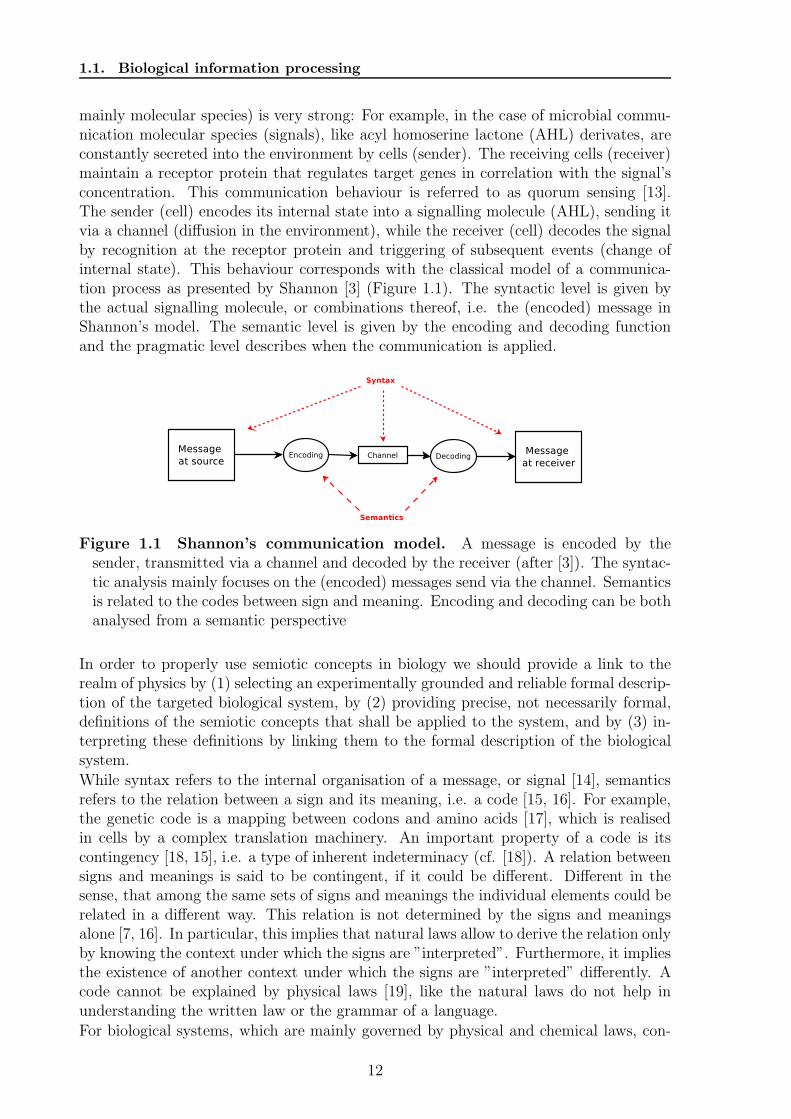
mainly molecular species) is very strong: For example, in the case of microbial commu-nication molecular species (signals), like acyl homoserine lactone (AHL) derivates, areconstantly secreted into the environment by cells (sender). The receiving cells (receiver)maintain a receptor protein that regulates target genes in correlation with the signal’sconcentration. This communication behaviour is referred to as quorum sensing [13].The sender (cell) encodes its internal state into a signalling molecule (AHL), sending itvia a channel (diffusion in the environment), while the receiver (cell) decodes the signalby recognition at the receptor protein and triggering of subsequent events (change ofinternal state). This behaviour corresponds with the classical model of a communica-tion process as presented by Shannon [3] (Figure 1.1). The syntactic level is given bythe actual signalling molecule, or combinations thereof, i.e. the (encoded) message inShannon’s model. The semantic level is given by the encoding and decoding functionand the pragmatic level describes when the communication is applied.
Figure 1.1 Shannon’s communication model. A message is encoded by thesender, transmitted via a channel and decoded by the receiver (after [3]). The syntac-tic analysis mainly focuses on the (encoded) messages send via the channel. Semanticsis related to the codes between sign and meaning. Encoding and decoding can be bothanalysed from a semantic perspective
In order to properly use semiotic concepts in biology we should provide a link to therealm of physics by (1) selecting an experimentally grounded and reliable formal descrip-tion of the targeted biological system, by (2) providing precise, not necessarily formal,definitions of the semiotic concepts that shall be applied to the system, and by (3) in-terpreting these definitions by linking them to the formal description of the biologicalsystem.
While syntax refers to the internal organisation of a message, or signal [14], semanticsrefers to the relation between a sign and its meaning, i.e. a code [15, 16]. For example,the genetic code is a mapping between codons and amino acids [17], which is realisedin cells by a complex translation machinery. An important property of a code is itscontingency [18, 15], i.e. a type of inherent indeterminacy (cf. [18]). A relation betweensigns and meanings is said to be contingent, if it could be different. Different in thesense, that among the same sets of signs and meanings the individual elements could berelated in a different way. This relation is not determined by the signs and meaningsalone [7, 16]. In particular, this implies that natural laws allow to derive the relation onlyby knowing the context under which the signs are ”interpreted”. Furthermore, it impliesthe existence of another context under which the signs are ”interpreted” differently. Acode cannot be explained by physical laws [19], like the natural laws do not help inunderstanding the written law or the grammar of a language.
For biological systems, which are mainly governed by physical and chemical laws, con-
12
Chapter 1. Introduction
tingency (sometimes called arbitrariness) need not necessarily to hold, but it is discussedwhether it is a useful concept [7, 20, 21, 18, 22]. While in language it comes naturally tous that we can change the object we denote by a word easily, in molecular systems wefirst have to understand the nature of the relation between signs and meanings. Con-tingency in molecular systems seems to stand in contrast to the rules of physics andchemistry which govern all molecular processes, because if the laws of physics explainevery process there would be no place for a contingency. The example of the geneticcode shows that this is not always the case. The relation between codons and aminoacids is realised by a sequence of reactions that are governed by chemical rules, but thechoice which codon is translated into which amino acid can be understood as arbitrary,or contingent. If we say codons (signs) are mapped to amino acids (meanings) then a(total) arbitrary mapping could in principle relate all signs to all meanings. This free-dom of assignment is also a property of the chemical system. There may be constraintsto the actual shape of the mapping, but as long as in principle the mapping could bechanged it can be considered to be contingent. Assuming a total contingent relationbetween signs and meanings is the most general state we can describe in this context.Barbieri identified these as (chemical) ”independent worlds” [16]. The contingency isimplemented in the structure of the adapter molecules that allows to connect these twoworlds.
In biological systems signs and meanings are molecular species (cp. [16, 23]). Con-tingency in a biological system needs to be identified among the relations between themolecular species in order to characterise a code, the semantic level of the biologicalsystem.
1.2 Related formal concepts
I will briefly review the concepts of code as used in Shannon’s ”Theory of communica-tion”, Tlusty’s ”molecular codes”, and Barbieri’s ”organic codes”.
The notion of code in information theory and coding theory. The first notionof code is often used when a combinatorial complexity is described, as for examplethe codons of the genetic code. This notion is related to the definition of ”code” asused in coding theory, a discipline of discrete mathematics. Coding theory studies theconstruction, parametric bounds, and implementation of (error-correcting) codes. Incoding theory a code C is a set of codewords from a common alphabet, C ⊂ A∗ (cp. [24]).Certain other conditions can be applied to such a code, for example, fixed length codewords, as for block codes. Implicitly, these codewords are situated in a communicationprocess between a sender, who needs to encode a message that has to be sent via achannel, and a receiver who needs to decode it. While coding theory mainly focusseson the structure and properties of the codewords, the second notion of code (code =mapping) refers to the process of encoding (decoding). It catches the relation betweena codeword and its ”meaning”.
Information theory utilises the second notion of code. Cover and Thomas, for example,defined a (source) code ”[..] C for a random variable X [as] a mapping from [..] therange of X, to [..] the set of finite length strings of symbols from a D-ary alphabet.” [25].This definition describes the encoding and is used, for example, in data compression.Alternatively, the decoding scheme is a mapping from the codewords to the ”message”.
13
1.2. Related formal concepts
In Shannon’s ”Theory of communication” [3] the messages to be send through the chan-nel are encoded before sending. The meaning of each message is irrelevant to the functionof the channel, and thus is also not captured by Shannon’s theory. The code, i.e. themapping between message and the encoded string of binary digit, keeps some impor-tance, e.g. it can be optimised with respect to the properties of the channel. Shannon’ssource coding theorem, for example, shows that the average number of bits per symbol(of the message) cannot be smaller than the channel’s entropy [3]. In computer scienceand mathematics ”coding theory” has been established as a field of study. It deals withthe engineering problem to identify optimal codes for applications in data compression,cryptography, or error-correction (cf. [26, 27] and references therein).
Beside this, the notion of code has been applied to biological research to understandhow information encoding in biological systems is employed.
A physical model molecular codes Tlusty describes molecular codes from a the-oretical, physical point of view [28]. In his framework he defines the sets of signs andmeanings beforehand and generally allows all signs to be mapped onto all meanings.This mapping is modelled as a transition matrix that gives the probabilities that a signa is mapped onto a meaning ω. The process of encoding and decoding is modelled asa Markov chain (see Figure 1.2). By defining cost and quality of a code he was ableto show that coding occurs as a phase transition[29]. The optimisation of the code viathe transition matrix accesses the semantic level (mapping between signs and meanings)from the pragmatic level (optimality, fitness). The coding state can be reached froma random, non-coding state by either increase in gain (bits of information to increasecode quality), an increased reading accuracy of the signals, a larger distance betweenthe meanings, or increase of population size [29].
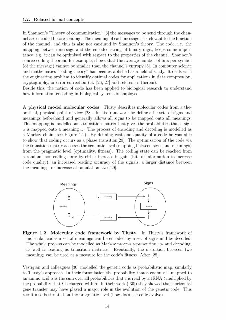
Figure 1.2 Molecular code framework by Tlusty. In Tlusty’s framework ofmolecular codes a set of meanings can be encoded by a set of signs and be decoded.The whole process can be modelled as Markov process representing en- and decoding,as well as reading as transition matrices. Eventually, the distortion between twomeanings can be used as a measure for the code’s fitness. After [28].
Vestigian and colleagues [30] modelled the genetic code as probabilistic map, similarlyto Tlusty’s approach. In their formulation the probability that a codon c is mapped toan amino acid α is the sum over all probabilities that c is read by a tRNA t multiplied bythe probability that t is charged with α. In their work ([30]) they showed that horizontalgene transfer may have played a major role in the evolution of the genetic code. Thisresult also is situated on the pragmatic level (how does the code evolve).
14
Chapter 1. Introduction
Organic codes Barbieri introduced the concept of ”organic codes” [31] as a semioticframework to explain the sign usage in biological systems. His definition of code requiresthree propositions to be met: There have to exist (1) two independent molecular worldsthat (2) are connected by a system of adapters that realise a (3) relation between ele-ments of the two worlds [16]. Independent molecular worlds, here, are characterised bychemically different molecular species, as for example in the genetic code where DNAis chemically different from the amino acids. This also implies that there is no directchemical relationship between these worlds, e.g. metabolic reactions. By his notion of”independent worlds” a relation between signs and meanings always needs to be con-tingent, because if the worlds are independent no chemical or physical law determinesthe mapping. The relation that is made between signs and meanings, i.e. the code, isrealised by the adapters. To identify an organic code the adapter molecules have to beidentified. An adapter molecule performs two independent recognition processes thatlink the two independent worlds. The genetic code, as organic code, connects DNA andamino acids (independent worlds), via the action of tRNAs. A tRNA molecule recog-nises the (complementary) RNA codon (first recognition) and carries the appropriateamino acids (second recognition). There exist a system of tRNAs that, taken together,implement the genetic code. The concept can be applied to other cellular subsystems,like splicing [31, 16].
The need for a formal definition of molecular codes Tlusty’s framework ofmolecular codes allows to derive general properties with respect to a code’s evolutionand fitness. But is does not help to identify a chemical system that allows for coding.Barbieri’s concept of organic codes, in principle, allows for the identification of a codewhen the independent world and the adapters can be identified. Nevertheless, a moreformal definition of molecular codes, that objectively can identify potential codes inchemical system, would be the next important step towards a code-based analysis ofbiological systems.In this thesis I will present a formal concept of molecular codes based on chemicalreaction networks. Chemical reaction networks are discrete models of actual biologicalor chemical systems. The grounding of a formal definition of molecular codes in anexplicit formal model of a system is, to the current state of the art, new.With this approach, the semiotic concept of code gets – at least partially – opera-tionalised by means of physical experiments. In particular, it allows to incorporatecontingency in a formal model of molecular codes.
1.3 Structure of the thesis
In the present chapter I gave a general introduction to the background of biologicalinformation processing and the motivation to develop formal models of otherwise looseconcepts. In Chapter 2 I will review three major biological systems that have beenreported to constitute a molecular code, i.e. the genetic code, the histone code, andthe sugar code. The chapter once again motivates the need for a more formal definitionof codes. Especially, in the histone code and the sugar code the notion of code isnot used homogeneously. In Chapter 3 I will present the definition of molecular codeswith respect to chemical reaction networks. I will also describe algebraic properties ofmolecular codes. The formal definition of molecular codes allows to develop algorithmsfor code identification. In Chapter 4 I will present two algorithms, one based on closed
15
1.3. Structure of the thesis
sets and one based on paths, to find all codes in a chemical reaction network anddiscuss the algorithms runtime properties. For the path based algorithm I proposetwo heuristic improvements, (1) by using the K-shortest paths, and (2) by a Monte-Carlo subnetwork sampling algorithm. In Chapter 5 I will present the results of theapplication of the algorithms to various biological and chemical systems. Chapter 6discusses how the presented structural semantic level can be extended and validated bythe pragmatic level. Finally, in Chapter 7 I will discuss further topics emerging fromthe presented formalism, algorithms, and results from actual networks. Appendix Acontains a collection of algorithms and helper methods I used for the code identifyingalgorithms. Appendix B contains the detailed proof of the ”ten closed sets” lemmaapplying to molecular codes. In Appendix C and D additional detail about resultsof a code based analysis of the human signal transduction network from the reactomedatabase 2 and a metabolic network extracted from the KEGG database 3 are given,respectively. The network models of all analysed systems are collected in Appendix E.
2www.reactome.org3www.genome.jp/kegg
16
Chapter 2
The notion of ”Code” in biologicalresearch
Parts of this chapter have been published in [32].
Comparing the literature on codes in biological systems shows that the term ”code” isused in two meanings, (1) as family of codewords, e.g. as in a block code, and (2) asmapping.
Both notions are used in recent biological literature, but not as formally defined as ininformation and coding theory (see Introduction). I will review three (major) biologicalsystems that have been described to constitute molecular codes. I will discuss the usednotion of code and give suggestions for a common usage of the term code as mappings.
2.1 Gene translation – The genetic code
The most prominent molecular code is the genetic code. In general the genetic codeis referred to as the association between codons and amino acids. This is realised byamino acyl-tRNA synthetases (aaRSs) (for reviews on the genetic code see [17] and onaaRSs chemistry see [33]). There exist twenty different aminoacyl-tRNA synthetases1,each one of them specific for one of the proteinogenic amino acids. A specific aaRSsrealises a particular association between a tRNA and an amino acid. The specificity ofthe recognition is implemented mainly by interaction with the anticodon of the tRNA[33]. The anticodon is, as the codon on the DNA/mRNA, a codeword which can bedescribed as an element of a block code of length 3, GCBlock = {A,C,G, T}3. Thus, thetRNA/aaRSs system implements a reading system for this block code, i.e., the set ofcodewords. The semantic code is the decoding scheme consisting of the set of codewords{AAA,AAC, . . . , TTT} and the mapping from this set to the set of amino acid symbols{Ala,Gly, . . . , T yr}. The tRNAs function as adaptors of the code by realising tworecognition processes (compare also [16]), i.e. between codon and tRNA and betweenamino acid and tRNA, and thereby realising the association between codon and aminoacid.
The appealing feature of the genetic code is its simplicity. The coding table shows onlythe decoding function, i.e., the semantic aspect of the gene translation system. Such asimple description, that abstracts from the complex biochemical processes of recognition,would also be desirable for other molecular codes.
1Sometimes aaRSs are also called “codases” since they are the enzymes that implement the code[33, 34]
17
2.2. Covalent histone modifications - The histone code
In a subsequent chapter (Chapter 5.5) the gene translation system will be analysed forits coding properties.
2.2 Covalent histone modifications - The histone code
Beside the genetic code other biological subsystems of the cell have been reported toconstitute or contain codes [16]. In this section I will describe the system of histonemodifications and discuss the possibility that it constitutes a molecular code.In all kingdoms of life the DNA is organized in some kind of superstructure, a kind ofpackaging. This packaging is mainly maintained by so called “chromosomal architecturalproteins” (chAPs), e.g., histones in eukaryotes. The existence of different modificationsites on the tails of the histones led to the hypothesis that histone modifications couldbe part of a complex code, the histone code. At the moment there exist two theorieshow histone modifications can have an effect on gene regulation [35, 36]. The firstone postulates a direct effect (in cis) of histone modifications on chromatin structureby altering the positive charge of the histone tails. The chromatin can regulate geneexpression by its structure [37]. Dense chromatine inhibits transcription, while an openchromatine structure allows for transcription. The transcription in the latter case ispossible because the DNA is accessible for the transcription machinery. Such an openingof the DNA at a histone can also be triggered by post-translational modifications ofthe histone tails. Certain modifications, like acetylations, can change the electrostaticproperties of the protein-DNA interaction [38] and thus allow for an opening of thechromatin structure. This charge neutralisation weakens the interaction of histone tailsand the DNA [38]. This theory applies only to acetylation and does not cover othertypes of modifications [35].The second theory, the histone code hypothesis, has been introduced by Turner [39, 40],and Strahl and Allis [41]. It proposes that histone modifications are recognised andtranslated into biological functions [42] mediated by adaptor proteins (in trans) [43]Talking about translation should refer to a decoding scheme, but from the definition andthe usage of the term “code” in this context it is not quite clear what exactly “code”should mean here, the combinatorial patterns of modifications [44] or the mapping. Inthe former case the histone code would only be a family of code words.From a semantic perspective the definition of a code must contain a mapping betweenthe set of codewords and the set of encoded meanings. So in case of the histone codethe codewords are modification patterns. But what are the meanings of the codewords,i.e., where are they mapped on? Different views have been reported, e.g., the modifica-tions are mapped on (1) “downstream functions” [41], (2) “regulation of transcriptionalactivity” [45, 46, 47], (3) “other histone modification patterns”[35, 48].In case of (1) the meanings could be high level functions, like meiosis, sporulation, etc.In case of (2) the meanings would basically be “on” and “off”. And in case of (3) themeanings would be other patterns of histone modifications. Each of these three caseswould constitute a different code.It has also been proposed to use terms such as “language” and “grammar” in the caseof histone cross-talk [36], but his does not contribute to a suitable description of thehistone code as long as both terms are in need of a proper definition.How could a histone code be realized by cells? Histone modifications can be activelywritten, read, and erased by protein domains [35, 36, 37]. (1) The combination of dif-ferent reader domains in one protein or protein complex allows for the recognition of
18
Chapter 2. The notion of ”Code” in biological research
not just single modifications, but patterns of modifications. This is for example the casefor a tandem bromodomain reading two acetylated histone amino acids [49]. (2) Thecombination of reader domains and effectors (e.g., writing domains, erasing domains, orother enzyme functionality) allows for the coupling to biological function. Both features(1) and (2) together can make up the core of a histone code, because it makes the for-mation of adaptors possible. Therefore, by combining different domains, the cell wouldbe able to read the codewords (patterns of modifications) of the histone code and relatethem to some biological function. For proteins in general this has been referred to as“compositional semantics” [11]. An example for probable adaptors is the family of BAFcomplexes which contains several Bromo- (acetylation recognition), Chromo- (methyla-tion recognition), and PHD-domains for combined modification recognition [50]. Themeanings of the code then are given by the biological effects, or functions that aredirectly linked to the actions mediated by the adaptors. Other effects or behaviours,located downstream, may also depend indirectly on the histone code.
2.3 Glycan recognition – The sugar code
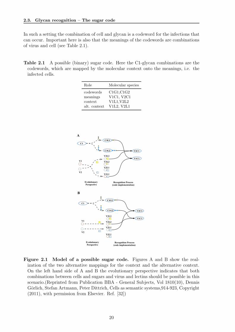
Another well-studied biological system has already been described in terms of code,i.e., the sugar code [51, 52, 53, 54]. Monosaccharids can by combined to glycans invarious ways, resulting in an enormous amount of different glycans. The huge numberof different combinations are supposed to be the code in the sugar code. Laine [55, 54]defined the coding capacity of the sugar code as number of combinations that can beformed with a fixed number of monosaccharids. E.g., ≈ 1015 different hexasaccharidscan be formed from 20 monosaccharids. This notion of coding capacity is based on theidea that the combinations of different building block make up the code. But from asemantic point of view it is necessary to define the code also by referring to a mappingbetween two sets of molecular species. Then the number of different oligosaccharidsalone does not constitute the coding capacity but is equal to the number of differentpossible codewords.The sugar code, as a semantic concept, has also to refer to the lectins. Lectins areproteins which recognize glycans, i.e., they are reading domains. There are many lectinsknown in bacteria and viruses [56], plants [57], and animals [58] so that it can be hy-pothesized that sugar codes are ubiquitously distributed. For a semantic description ofa possible sugar code I will present a simple abstract model of virus-cell recognition,which is based on some artificial assumptions. The model starts from the known factthat viruses uses lectins to recognise glycans, which are presented on the cell surface [59].I here assume a system with two glycans (G1,G2), one species of cells (C1), two viruses(V1,V2), and two lectins (L1,L2). From an evolutionary perspective the cells can be com-bined with both sugars resulting in the cell-glycan combinations (C1G1,C1G2), whilethe viruses could evolve to utilise both lectins, resulting in (V1L1,V1L2,V2L1,V2L2).We assume here that the lectins are specific, such that lectin 1 may only bind to glycan1, and lectin 2 only to glycan 2. Thereby we may also get all infection combinations ofvirus and cells (V1C1, V2C1). In such a system a code can be identified. It containsthe decoding function between the combinations of cells and glycans (C1G1,C1G2) andthe infected cells (V1C1,V2C1). The decoding function is realized by the virus-lectincombinations (V1L1,V2L2), which we could call “codemakers” following a suggestion of[31], or molecular contexts of the mapping. There exists an alternative set of combina-tions (V2L1,V1L2), i.e. context, realizing a different decoding function (see Figure 2.1).
19
2.3. Glycan recognition – The sugar code
In such a setting the combination of cell and glycan is a codeword for the infections thatcan occur. Important here is also that the meanings of the codewords are combinationsof virus and cell (see Table 2.1).
Table 2.1 A possible (binary) sugar code. Here the C1-glycan combinations are thecodewords, which are mapped by the molecular context onto the meanings, i.e. theinfected cells.
Role Molecular species
codewords C1G1,C1G2meanings V1C1, V2C1context V1L1,V2L2alt. context V1L2, V2L1
Figure 2.1 Model of a possible sugar code. Figures A and B show the real-ization of the two alternative mappings for the context and the alternative context.On the left hand side of A and B the evolutionary perspective indicates that bothcombinations between cells and sugars and virus and lectins should be possible in thisscenario.(Reprinted from Publication BBA - General Subjects, Vol 1810(10), DennisGorlich, Stefan Artmann, Peter Dittrich, Cells as semantic systems,914-923, Copyright(2011), with permission from Elsevier. Ref. [32])
20
Chapter 2. The notion of ”Code” in biological research
2.4 Summary
The review of three systems discussed as codes in the literature shows that a properformalised notion of codes is needed to foster that terms are used similarly. While forthe genetic code it is commonly accepted that codons are mapped onto amino acids.For the other presented systems a clearer definition what the code is based on biologicalevidences would be also important. Best, the notion of code follows objective definitions.These are helpful to distinguish between the code, the code’s execution, its evolutionand pragmatics, the signs and the meanings in the code. Only the formal definition ofcode enables us to objectively discuss these in the various systems mentioned here.The discussion of the biological systems also showed that the alphabet from which poten-tial codewords are formed can be very heterogeneous. For example, to define the histonecode’s codewords the type of the covalent modification and its position is important,limited to the ability of the reading systems to recognize (complex) codewords.
21

2.4. Summary
22
Chapter 3
A formalisation of molecular codes
Parts and ideas of the contents presented in this chapter have been published in [60].
To access the notion of molecular codes for chemical and biological systems it is necessaryto define it formally, best in a mathematical manner. This chapter introduces the formalframework for code based network analysis.
3.1 Formalisation of molecular codes in chemical re-
action networks
Reaction networks are a suitable abstraction level to model systems of various kind. Inthe following I will define reaction networks (Def. 3.1.1), closed sets (Def. 3.1.4), paths(Defs. 3.1.2), because these concepts are important for the algorithmic identification ofmolecular codes.
Chemical reaction network Chemical reaction networks are usually defined by itsmolecular species, the reactions among these species and the kinetic laws governingthe reactions (cf. [61]). For the definition of molecular codes I model only the staticstructure of a system as reaction network, such that the following definitions neglectskinetic information1.
Definition 3.1.1 (reaction network). A chemical reaction network N = (M,R) is atuple of a set of molecular species M and a set of reactions R given by R ⊆ P(M) ×P(M) that can happen among the elements of M. Each reaction ρ ∈ R is defined byits reactants lρ ∈ P(M) and products rρ ∈ P(M).
Paths Intuitively, the molecular species of a reaction network N , eventually, are re-lated by paths of reactions in the network. This allows to define relations among molec-ular species later on.
Definition 3.1.2 (s-t path). Given a reaction network N = (M,R) a path p =(ρ1, ρ2, . . . , ρi, . . . , ρn) with ρi ∈ R is an ordered tuple of n reactions. In particular,the molecular species s ∈ M is called start species s ∈ lρ1 and t ∈ M is called targetspecies t ∈ rρn. For all sequential pairs of reactions ρi, ρi+1, i ∈ {1, 2, . . . , n−1} it shouldhold that at least one element of rρi is also in lρi+1
:
∀i ∈ {1, 2, . . . , n− 1} : ∃mi ∈ rρi ∧mi ∈ lρi+1.
1Kinetic information can be reintroduced later, e.g. for the pragmatic level, see Section 6
23
3.1. Formalisation of molecular codes in chemical reaction networks
Corollary 3.1.1 (species s-t path). Each path in N = (M,R) induces a species pathpst = (s,m1, m2, . . . , mi, . . . , mk, t) with s, t,mi ∈M as ordered tuple of k + 2 species.
Corollary 3.1.2. A species path pst = (s,m1, m2, . . . , mj , . . . , mn−2, t) of length n in-duces a reaction path pρ1ρn−1
of length n− 1, iff there exists n− 1 reactions ρi ∈ R, suchthat s ∈ lρ1 , t ∈ rρn−1 , mj ∈ rρj , mj ∈ lρj+1
, with j ∈ {1, 2, . . . , n− 2}.
Both notions of paths can be constructed from each other (Corollary 3.1.2), such that Iwill use the notion of path for the rest of this thesis and will refer to reactions or speciesas needed.
Molecular context In the following I will introduce the notion of the molecular con-texts of a path. If a path from species s to species t does not only consist of spontaneousreactions a non-empty molecular context for this path can be identified. Following thereactions from s to t some of the reactants are produced by the preceding reactions,but some additional species may be necessary to execute all reactions among the path.I will call the set of these necessary molecular species ”molecular context”. In otherwords: The contexts consists of all molecular species that are not produced by a path,but necessary for the execution of the reactions.
Definition 3.1.3 (molecular context). Every s-t path induces a molecular context Cwhich is necessary to execute the reactions on the path. For a path among species(m1, m2, . . . , mn) and reactions (ρ1, ρ2, . . . , ρn−1) the context is given by
C =
n−1⋃
i=1
lρi −mi
For a given reaction network a particular path has only one context, because the path,by definition, has only one starting species and a defined set of reaction. The startingspecies and the set of reactions define the context.
Closed sets A useful concept to access the substructure of a reaction network is thenotion of closed sets (cf. [62]). Intuitively, a closed set is set of molecular species thatcannot produce ”new” species that are not already contained in the set, thus, it staysclosed.
Definition 3.1.4 (closed set). Given a reaction network N = (M,R) and a subsetA ∈ M we say A is closed, iff for all reactions that can happen among the molecularspecies in A no new species are produced. If A is closed it holds that
∀ρ ∈ R : lρ ⊆ A→ rρ ⊆ A.
The smallest closed set of an initial set A is called closure of A. The closure for anygiven set A can be calculated by the GCL() operator (Algorithm A.5). Algorithm A.3gives the set of all closed sets ClN .
24
Chapter 3. A formalisation of molecular codes
A reaction network that contains the species A,B,C and one reaction, e.g. A+B → Ccontains two paths (A,C) and (B,C). The molecular context for path (A,C) is {B}and the molecular context for path (B,C) is {A}. It also contains five closed setsCl = {∅, {A}, {B}, {C}, {A,B,C}}.
Definition 3.1.5 (single molecule closed set). Given a reaction network N = (M,R)the set of single molecule closed sets of N is defined as
SclN = {c ∈ ClN |c = GCL(m), m ∈M} .
To define a molecular code I will start to define a molecular relation and a molecularmapping. In particular, a molecular code is a special case of a molecular mapping, whichis a special case of a molecular relation.The general definition of ”relation”, following [63], is:
Definition 3.1.6 (relation). Given two set A and B. A relation R is a subset of A×B,
R ⊆ A× B. (3.1)
For a reaction network N a relation RN among the molecular species is given by RN ⊆M×M.
Definition 3.1.7 (molecular mapping). Given a reaction network N = (M,R) and
two sets of molecular species A,B ⊆M, we say that f : AC7→ B is a molecular mapping
with respect to N , iff there exists a relation
F = {(a, b) ∈ A× B|a path p = (a, . . . , b) exists in N} (3.2)
which is left-total ∀a ∈ A∃b ∈ B : (a, b) ∈ Fand right-unique ∀a ∈ A, b, c ∈ B : (a, b) ∈ F ∧ (a, c) ∈ F → b = cwith p realised by C ⊆M (called context).
The left totality requires that all elements from the domain are used in the mapping,while right-uniqueness guarantees that no element of the domain maps to two elementsfrom the codomain.Alternatively closed set can be used to define a molecular mapping by defining
F = {(a, b) ∈ A× B|b ∈ GCL(a ∪ C)}. (3.3)
The calculation of the closure operator implies a repeated application of the operator toa set of molecular species. In each step the operator applies all possible reaction rules.By this the sequence of reactions leading to b is generated and also the s-t path. If thereexists a molecular mapping f with respect to N , N can realise the molecular mappingf .Note that in a reaction network there is usually more than one molecular context Cthat realises a particular molecular mapping f . Intuitively, in order to “compute” f(a)with the reaction network N , we put all molecules from the context C together with aand repeatedly apply all applicable reaction rules until no novel molecular species canbe added any more. Then it is checked which molecular species from the codomain B is
25
3.2. Binary molecular codes
present, which must be – according to Definition 3.1.7 – only one species and the resultof f(a).Based on the notion of a molecular mapping a molecular code can be defined. As outlinedin the introduction, a code is a mapping between sets of objects, where the mappingcould be different. To identify different mappings the alternative contexts needs to beidentified.
Definition 3.1.8 (molecular code). Given a reaction network N = (M,R) and a non-
constant2 molecular mapping f : AC7→ B, with A,B,C ⊆ M we call the mapping f
a molecular code with respect to N , if all other mappings gi : AC′
i7→ B with the samedomain A and codomain B can also be realised by the reaction network N , i.e., thereexist alternative molecular contexts C ′i to map A to B.
The definition implements the notion of contingency, i.e. the elements of the domaincan be mapped to the elements of the codomain in every possible way by changingthe molecular context. Thus, networks that contain molecular codes realise an encodedrelationship between molecular species by choosing or regulating a molecular context.Each code implies a family of potential molecular codes that are only distinguished bytheir molecular contexts. From these alternative mappings only few, perhaps only one,is realised in the systems that can be observed nowadays. If more than one of thealternative codes would be realised at the same time in the same system the mappingwould not be right-unique, i.e. the mapping is no function any more.The identification of a code, using our framework, does not guarantee that this particularcode can be realised in the system. To finally verify a code’s existence the pragmatic levelneeds to be added. On the pragmatic level the system has to choose, either by evolution,or by regulatory control, one of the alternative mappings to obtain a unique mapping(cf. Section 6). The identification of a code is a first measure if the (biochemical) systemin principle could implement contingent mappings.
3.2 Binary molecular codes
In order to keep this study tractable, I will focus on molecular codes that are binary,i.e., where domain as well as codomain contain exactly two molecular species [60]. Iwill also not study molecular mappings that are only partially contingent. For binarymolecular codes the definition can be reformulated as follows:
Definition 3.2.1 (binary molecular code). Given a reaction network N = (M,R) andtwo binary sets of molecular species A = {a1, a2} ⊆ M and B = {b1, b2} ⊆ M. The
molecular mapping f : AC7→ B is called binary molecular code (BMC), iff there exist
two sets C,C ′ ⊆M, such that the following conditions hold:
f(a1) ∈ GCL({a1} ∪ C), and f(a2) /∈ GCL({a1} ∪ C), and
f(a2) ∈ GCL({a2} ∪ C), and f(a1) /∈ GCL({a2} ∪ C), and
f(a2) ∈ GCL({a1} ∪ C ′), and f(a1) /∈ GCL({a1} ∪ C ′), and
f(a1) ∈ GCL({a2} ∪ C ′), and f(a2) /∈ GCL({a2} ∪ C ′).
2A mapping f : A→ B is called non-constant, iff there exists a, a′ ∈ A such that f(a) 6= f(a′).
26
Chapter 3. A formalisation of molecular codes
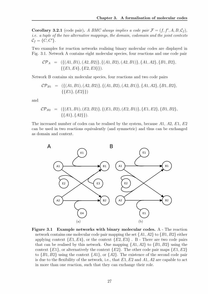
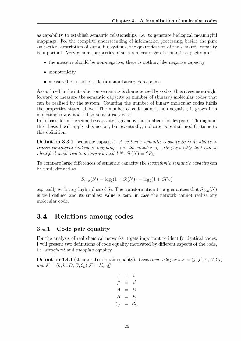
Corollary 3.2.1 (code pair). A BMC always implies a code pair F = (f, f ′, A, B, Cf),i.e. a tuple of the two alternative mappings, the domain, codomain and the joint contextsCf = {C,C ′}.Two examples for reaction networks realising binary molecular codes are displayed inFig. 3.1. Network A contains eight molecular species, four reactions and one code pair
CPA = ({(A1, B1), (A2, B2)}, {(A1, B2), (A2, B1)}, {A1, A2}, {B1, B2},{{E1, E4}, {E2, E3}}).
Network B contains six molecular species, four reactions and two code pairs
CPB1 = ({(A1, B1), (A2, B2)}, {(A1, B2), (A2, B1)}, {A1, A2}, {B1, B2},{{E1}, {E2}})
and
CPB2 = ({(E1, B1), (E2, B2)}, {(E1, B2), (E2, B1)}, {E1, E2}, {B1, B2},{{A1}, {A2}}).
The increased number of codes can be realised by the system, because A1, A2, E1, E2can be used in two reactions equivalently (and symmetric) and thus can be exchangedas domain and context.
(a) (b)
Figure 3.1 Example networks with binary molecular codes. A - The reactionnetwork contains one molecular code pair mapping the set {A1, A2} to {B1, B2} eitherapplying context {E1, E4}, or the context {E2, E3} . B - There are two code pairsthat can be realised by this network. One mapping {A1, A2} to {B1, B2} using thecontext {E1}, or alternatively the context {E2}. The other code pair maps {E1, E2}to {B1, B2} using the context {A1}, or {A2}. The existence of the second code pairis due to the flexibility of the network, i.e., that E1, E2 and A1, A2 are capable to actin more than one reaction, such that they can exchange their role.
27
3.3. Semantic capacity
Lemma 3.2.1 (Ten unique closed sets). Given an BMC according to Definition 3.2.1the ten closures GCL(s1), GCL(s2), GCL(m1), GCL(m2), GCL(C), GCL(C
′), GCL(s1 ∪ C) =GCL(s1 ∪C ∪m1), GCL(s2 ∪C) = GCL(s2 ∪C ∪m2), GCL(s1 ∪C ′) = GCL(s1 ∪C ′ ∪m2),and GCL(s2 ∪ C ′) = GCL(s2 ∪ C ′ ∪m1) must be different.
If two of the above listed closed sets are not different the coding property vanishes,i.e. the signs or meanings get undistinguishable, or the relation is not unique becauseboth meanings are generated at the same time. I call these situations sign, or meaningdegenerated, respectively. A third form is that the contexts produce each other, i.e.the relation is context degenerated. For the proof by enumeration see Appendix B onpage 117.Lemma 3.2.1, leads to the conclusion that a network needs to be minimally structuredin the sense that enough (> 10) different closed sets exists. This is, for example, notthe case in a system where all the reactions happen spontaneously.
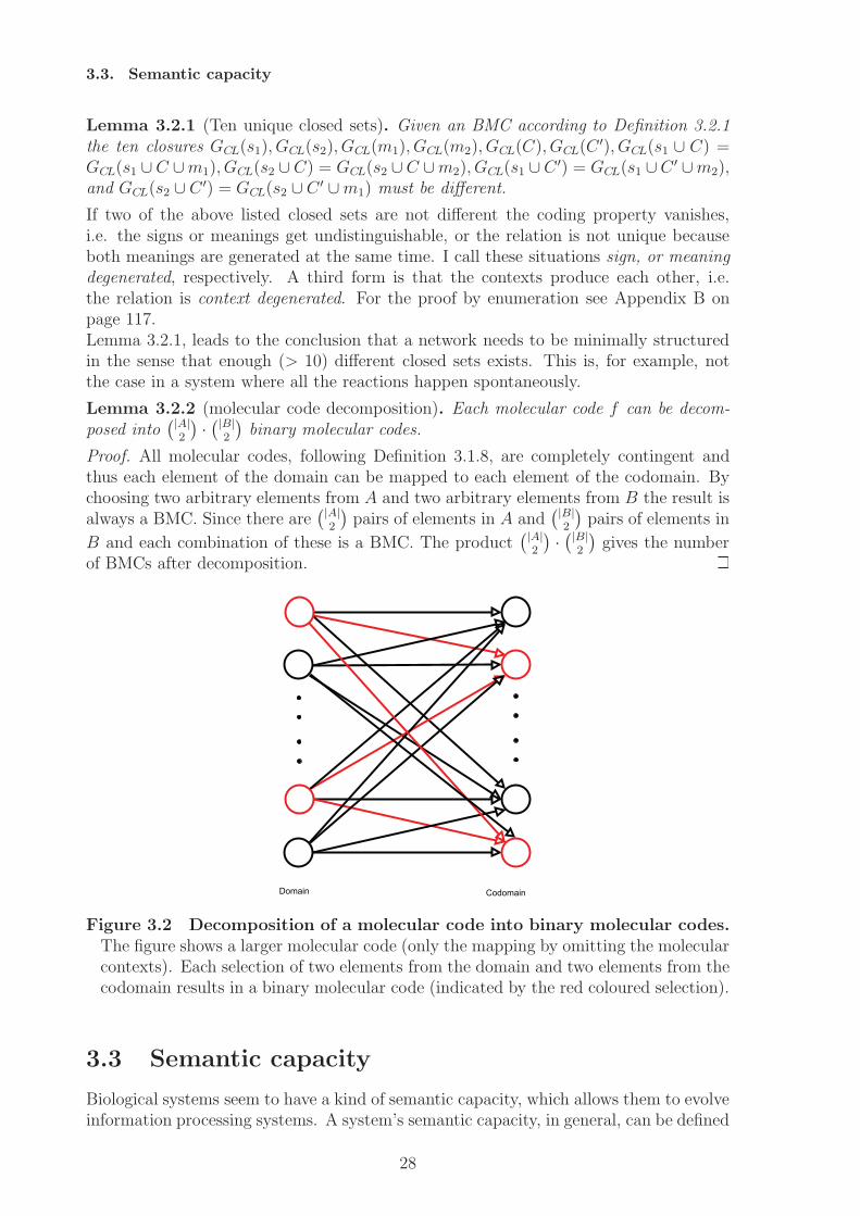
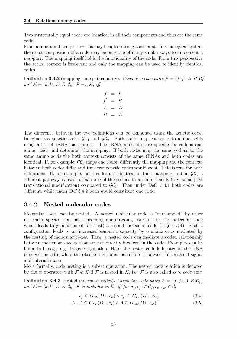
Lemma 3.2.2 (molecular code decomposition). Each molecular code f can be decom-posed into
(|A|2
)·(|B|2
)binary molecular codes.
Proof. All molecular codes, following Definition 3.1.8, are completely contingent andthus each element of the domain can be mapped to each element of the codomain. Bychoosing two arbitrary elements from A and two arbitrary elements from B the result isalways a BMC. Since there are
(|A|2
)pairs of elements in A and
(|B|2
)pairs of elements in
B and each combination of these is a BMC. The product(|A|2
)·(|B|2
)gives the number
of BMCs after decomposition.
Domain Codomain
Figure 3.2 Decomposition of a molecular code into binary molecular codes.The figure shows a larger molecular code (only the mapping by omitting the molecularcontexts). Each selection of two elements from the domain and two elements from thecodomain results in a binary molecular code (indicated by the red coloured selection).
3.3 Semantic capacity
Biological systems seem to have a kind of semantic capacity, which allows them to evolveinformation processing systems. A system’s semantic capacity, in general, can be defined
28
Chapter 3. A formalisation of molecular codes
as capability to establish semantic relationships, i.e. to generate biological meaningfulmappings. For the complete understanding of information processing, beside the puresyntactical description of signalling systems, the quantification of the semantic capacityis important. Very general properties of such a measure Sc of semantic capacity are:
• the measure should be non-negative, there is nothing like negative capacity
• monotonicity
• measured on a ratio scale (a non-arbitrary zero point)
As outlined in the introduction semantics is characterised by codes, thus it seems straightforward to measure the semantic capacity as number of (binary) molecular codes thatcan be realised by the system. Counting the number of binary molecular codes fulfilsthe properties stated above: The number of code pairs is non-negative, it grows in amonotonous way and it has no arbitrary zero.In its basic form the semantic capacity is given by the number of codes pairs. Throughoutthis thesis I will apply this notion, but eventually, indicate potential modifications tothis definition.
Definition 3.3.1 (semantic capacity). A system’s semantic capacity Sc is its ability torealise contingent molecular mappings, i.e. the number of code pairs CPN that can beidentified in its reaction network model N , Sc(N) = CPN .
To compare large differences of semantic capacity the logarithmic semantic capacity canbe used, defined as
Sclog(N) = log2(1 + Sc(N)) = log2(1 + CPN)
especially with very high values of Sc. The transformation 1+x guarantees that Sclog(N)is well defined and its smallest value is zero, in case the network cannot realise anymolecular code.
3.4 Relations among codes
3.4.1 Code pair equality
For the analysis of real chemical networks it gets important to identify identical codes.I will present two definitions of code equality motivated by different aspects of the code,i.e. structural and mapping equality.
Definition 3.4.1 (structural code pair equality). Given two code pairs F = (f, f ′, A, B, Cf)and K = (k, k′, D, E, Ck) F = K, iff
f = k
f ′ = k′
A = D
B = E
Cf = Ck.
29
3.4. Relations among codes
Two structurally equal codes are identical in all their components and thus are the samecode.From a functional perspective this may be a too strong constraint. In a biological systemthe exact composition of a code may be only one of many similar ways to implement amapping. The mapping itself holds the functionality of the code. From this perspectivethe actual context is irrelevant and only the mapping can be used to identify identicalcodes.
Definition 3.4.2 (mapping code pair equality). Given two code pairs F = (f, f ′, A, B, Cf)and K = (k, k′, D, E, Ck) F =m K, iff
f = k
f ′ = k′
A = D
B = E.
The difference between the two definitions can be explained using the genetic code.Imagine two genetic codes GC1 and GC2. Both codes map codons onto amino acidsusing a set of tRNAs as context. The tRNA molecules are specific for codons andamino acids and determine the mapping. If both codes map the same codons to thesame amino acids the both context consists of the same tRNAs and both codes areidentical. If, for example, GC2 maps one codon differently the mapping and the contextsbetween both codes differ and thus two genetic codes would exist. This is true for bothdefinitions. If, for example, both codes are identical in their mapping, but in GC2 adifferent pathway is used to map one of the codons to an amino acids (e.g. some posttranslational modification) compared to GC1. Then under Def. 3.4.1 both codes aredifferent, while under Def 3.4.2 both would constitute one code.
3.4.2 Nested molecular codes
Molecular codes can be nested. A nested molecular code is ”surrounded” by othermolecular species that have incoming our outgoing reactions to the molecular codewhich leads to generation of (at least) a second molecular code (Figure 3.4). Such aconfiguration leads to an increased semantic capacity by combinatorics mediated bythe nesting of molecular codes. Thus, a nested code can mediate a coded relationshipbetween molecular species that are not directly involved in the code. Examples can befound in biology, e.g., in gene regulation. Here, the nested code is located at the DNA(see Section 5.6), while the observed encoded behaviour is between an external signaland internal states.More formally, code nesting is a subset operation. The nested code relation is denotedby the ⋐ operator, with F ⋐ K if F is nested in K, i.e. F is also called core code pair.
Definition 3.4.3 (nested molecular codes). Given the code pairs F = (f, f ′, A, B, Cf)and K = (k, k′, D, E, Ck) F is included in K, iff for cf , cf ′ ∈ Cf , ck, ck′ ∈ Ck
cf ⊆ GCL(D ∪ ck) ∧ cf ′ ⊆ GCL(D ∪ ck′) (3.4)
∧ A ⊆ GCL(D ∪ ck) ∧A ⊆ GCL(D ∪ ck′) (3.5)
30
Chapter 3. A formalisation of molecular codes
By the conditions in Def. 3.4.3 it is guaranteed, that if F ⋐ K then in K the reactionsthat realise F are used, i.e. F is completely contained in K. This can either happen ifcf ⊆ ck or if the reactions among the outer code produce the domain and the context ofthe inner code. For Eq. (3.4) we can assume, without loss of generality, that the subsetsof Cf and Cg are sorted, such that cf ⊆ cg ∧ cf ′ ⊆ ck′ is true.
Here I present which properties, e.g. reflexivity, are fulfilled by the nested code relation.
Lemma 3.4.1 (nested code reflexivity). Given a code pair F = (f, f ′A,B, Cf = {cf , cf ′}),then F is always its own core code, i.e. F ⋐ F .
Proof. For Eq. (3.4) we get cf ⊆ GCL(D ∪ cf) ∧ cf ′ ⊆ GCL(D ∪ cf ′), which always holdfor equality, since the GCL operator does only increase the initial set. For Eq (3.5) weget A ⊆ GCL(A∪ cf ) which is by definition of GCLalways true using the same argument.Thus, F ⋐ F is always true.
I continue by showing transitivity.
Lemma 3.4.2 (nested code transitivity). Given three molecular code pairs
F = (f, f ′, A, B, Cf = {cf , cf ′}) ,G = (g, g′, D, E, Cg = {cg, cg′}) ,
and H = (h, h′, I, J, Ch = {ch, ch′})
we say the binary relation ⋐ among F ,G and H is transitive if
F ⋐ G ∧ G ⋐ H → F ⋐ H. (3.6)
I will only proof the lemma for one of the alternative molecular contexts. The proof forthe second alternative is equivalent, but decreases readability, here.
Proof. We can directly proof this lemma using the equations from the definition 3.4.3.For Eq (3.4) we need to show that the following implications (which arises from (3.6))hold.
cf ⊆ GCL(D ∪ cg) ∧ cg ⊆ GCL(I ∪ ch)→ cf ⊆ GCL(I ∪ ch) (3.7)
A ⊆ GCL(D ∪ cg) ∧D ⊆ GCL(I ∪ ch)→ A ⊆ GCL(I ∪ ch) (3.8)
To proof the implications we assume that the left hand sides of (3.7) and (3.8) are trueand show that the right hand sides then also always are true. For Eq. (3.7) we knowthat D, cg ⊆ GCL(I ∪ cg) = GCL(I ∪ cg ∪ D ∪ cg). Since the GCLoperator applies allpossible reaction rules to the initial set GCL(D∪cg) is also a subset of GCL(I ∪cg). Thusbecause of A, cf ⊆ GCL(D ∪ cg) and GCL(D ∪ ch) ⊆ GCL(I ∪ ch) we get
A, cf ⊆ GCL(D ∪ cg) ⊆ GCL(I ∪ ch)→ A, cf ⊆ GCL(I ∪ ch)
which proofs, by standard set theory, Lemma 3.4.2.
31
3.4. Relations among codes
A
B
cf
cg
D
E
I
J
ch
cg
D
E
A
B
cf
I
J
ch
cg
D
E
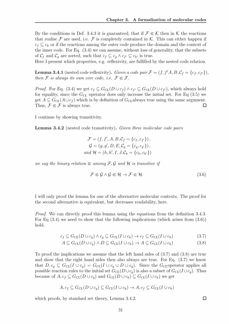
Figure 3.3 Subsets of transitive nested BMCs. The figure illustrates the prooffor core code transitivity. On the left hand side the initial situation is displayed, i.e.F (red) is a core code of G (green) and G is nested in H (blue). Thus applying theclosure operator to the initial subsets (dotted lines) generates a closed set containingthe codomain of the larger code and the context and domain of the nested code, andtherefore also the codomain of the nested code (solid coloured lines). Because allcomponents of F are generated by G and all components of G are generated by H, Fis nested in H.
The proof holds also for the alternative molecular codes.So far I have proven that the core code relation is always reflexive and transitive.The symmetry F � G ⇒ G � F for F = G is not valid in general. In actual networksthere may be situations where symmetrically nested codes occur. This can happen ifthe molecular contexts are not identical, but share a core mechanism which realises thecode. These codes are then very similar, if not the same code (reflexivity).Also antisymmetry, F � G ∧ G � F → F = G, is not always given for the nested coderelation. This is due to the fact that the two code pairs can be nested, but their contextsmay differ, such that the equality does not hold here.
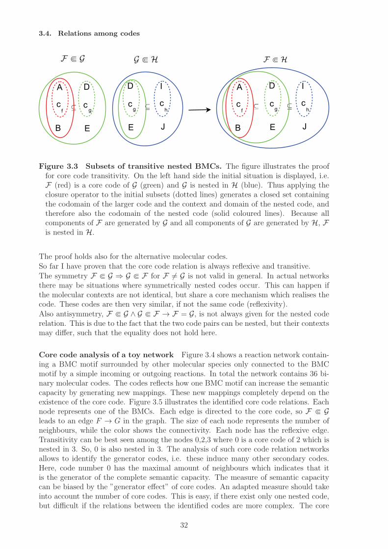
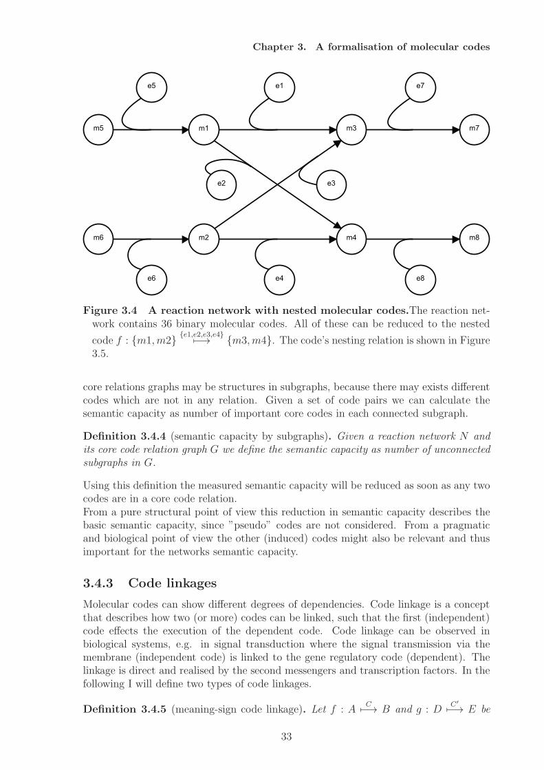
Core code analysis of a toy network Figure 3.4 shows a reaction network contain-ing a BMC motif surrounded by other molecular species only connected to the BMCmotif by a simple incoming or outgoing reactions. In total the network contains 36 bi-nary molecular codes. The codes reflects how one BMC motif can increase the semanticcapacity by generating new mappings. These new mappings completely depend on theexistence of the core code. Figure 3.5 illustrates the identified core code relations. Eachnode represents one of the BMCs. Each edge is directed to the core code, so F � Gleads to an edge F → G in the graph. The size of each node represents the number ofneighbours, while the color shows the connectivity. Each node has the reflexive edge.Transitivity can be best seen among the nodes 0,2,3 where 0 is a core code of 2 which isnested in 3. So, 0 is also nested in 3. The analysis of such core code relation networksallows to identify the generator codes, i.e. these induce many other secondary codes.Here, code number 0 has the maximal amount of neighbours which indicates that itis the generator of the complete semantic capacity. The measure of semantic capacitycan be biased by the ”generator effect” of core codes. An adapted measure should takeinto account the number of core codes. This is easy, if there exist only one nested code,but difficult if the relations between the identified codes are more complex. The core
32
Chapter 3. A formalisation of molecular codes
m1
m2
m3
m4
m5
m6
m7
m8
e1
e2 e3
e4
e5
e6
e7
e8
Figure 3.4 A reaction network with nested molecular codes.The reaction net-work contains 36 binary molecular codes. All of these can be reduced to the nested
code f : {m1, m2} {e1,e2,e3,e4}�−→ {m3, m4}. The code’s nesting relation is shown in Figure3.5.
core relations graphs may be structures in subgraphs, because there may exists differentcodes which are not in any relation. Given a set of code pairs we can calculate thesemantic capacity as number of important core codes in each connected subgraph.
Definition 3.4.4 (semantic capacity by subgraphs). Given a reaction network N andits core code relation graph G we define the semantic capacity as number of unconnectedsubgraphs in G.
Using this definition the measured semantic capacity will be reduced as soon as any twocodes are in a core code relation.From a pure structural point of view this reduction in semantic capacity describes thebasic semantic capacity, since ”pseudo” codes are not considered. From a pragmaticand biological point of view the other (induced) codes might also be relevant and thusimportant for the networks semantic capacity.
3.4.3 Code linkages
Molecular codes can show different degrees of dependencies. Code linkage is a conceptthat describes how two (or more) codes can be linked, such that the first (independent)code effects the execution of the dependent code. Code linkage can be observed inbiological systems, e.g. in signal transduction where the signal transmission via themembrane (independent code) is linked to the gene regulatory code (dependent). Thelinkage is direct and realised by the second messengers and transcription factors. In thefollowing I will define two types of code linkages.
Definition 3.4.5 (meaning-sign code linkage). Let f : AC�−→ B and g : D
C′
�−→ E be
33
3.4. Relations among codes
2713
1426
1215
24
34
28
9
35
31
32
25
30
17
719
18
16 4
529
20
6
21
23
8
33
22
10
1
11
0
2
3
Figure 3.5 Core code relation network of Fig. 3.4. The graph shows which codeis core code of which other code. There exists many core code relations. In particular,node number 0 is connected to every other node and thus is a kind of generator of allother codes. The size of the nodes represents the number of neighbors in the graph.Red nodes have a very high avg. connectivity, while green nodes have a lower avg.connectivity
molecular codes. g is linked directly to f , iff D is a subset of B.
g ≺MSCL f : D ⊆ B
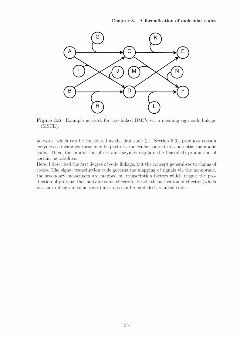
A meaning-sign code linkage (MSCL) can be observed for example in the gene regulatorysystem. Here the gene translation, i.e. the genetic code, is dependent on the output ofthe gene regulatory code (see section 5.6). The direct relationship comes into existence,because the output of the gene regulatory code, i.e. gene transcripts, is the input of thegenetic code. Because the gene transcript is a sequence of codons the genetic code hasto be executed several times, but in general they are directly linked.MSCL increases the semantic capacity as measured by code pairs. Since through thelinkage combinations of signs and meanings from f (which are signs from g) can be amolecular code mapping to the meanings of g. Figure 3.6 shows a MSCL situation, i.e.two linked BMC motifs. The network contains 23 BMCs.
Definition 3.4.6 (meaning-controlled molecular codes). Let f : AC�−→ B and g : D
C′
�−→E be molecular codes. g is controlled by f , iff C ′ is a subset of B.
g ≺MCMC f : C ′ ⊆ B
Meaning controlled molecular codes (MCMC) describe the linkage, where the meaning ofthe first codes are elements of the molecular context of the second code and thus, by theirpresence, regulate the execution of the second code. Situations which might be governedby such a code linkage may be found in metabolic regulation. If a gene regulatory
34
Chapter 3. A formalisation of molecular codes
A
B
C
D
E
F
G
H
I J
K
L
NM
Figure 3.6 Example network for two linked BMCs via a meaning-sign code linkage(MSCL).
network, which can be considered as the first code (cf. Section 5.6), produces certainenzymes as meanings these may be part of a molecular context in a potential metaboliccode. Then, the production of certain enzymes regulate the (encoded) production ofcertain metabolites.Here, I described the first degree of code linkage, but the concept generalises to chains ofcodes. The signal transduction code governs the mapping of signals via the membrane,the secondary messengers are mapped on transcription factors which trigger the pro-duction of proteins that activate some effectors. Beside the activation of effector (whichis a natural sign in some sense) all steps can be modelled as linked codes.
35

3.4. Relations among codes
36
Chapter 4
Algorithmic code identification
Parts and first ideas of the contents presented in this chapter have been published in [60] and [32].
The formal definition of a binary molecular code (Def. 3.2.1) allows the formulation ofsuitable algorithms to identify BMCs in reaction networks. Here two algorithms forcode identification are described, taking advantage of different properties of reactionnetworks, i.e. the number of closed sets and the pathways through the network. Bothalgorithms are directly derived from the definition of a BMC and follow a brute-forcestrategy by checking all combinations of either closed sets or molecular species for thecode conditions.
Important for the successful identification of codes in reaction network model is thatthe model contains the alternative mappings. For several reasons network models avail-able today does not contain all the alternative mappings. Before presenting the codeidentification algorithms I will discuss how suitable network models can be obtained.
4.1 Network representation
Today, network models of many biological systems are available from databases and canbe downloaded in standardised formats like SBML [64, 65].
All formats have in common that the system’s components needs to be represented inthe network description. Network structure is mainly represented as list of molecularspecies and list of reactions among the species.
While modern file formats are mostly based on XML and thus contain also many an-notations, e.g. kinetic information, I will here use a simplified network format, calledREA-format, describing only the network structure. A rea-file (.rea) contains a list ofmolecular species, the number of molecular species, a list of reactions including stoichio-metric coefficients and the number of reactions, in a plain text format. For compatibilitythe software can also use SBML Level 2 Version 1 files.
4.2 Obtaining suitable reaction networks
Classically, reaction networks are used to model actual biological or chemical systems.The network contains only the molecular species and reaction that have been observedbefore in the modelled system. Such networks, thus, can be called realised reactionnetworks. The set of realised reaction networks is a subset of all possible potentialnetworks that could have been realised.
37
4.3. Closure-based algorithm
The notion of contingency used in the code definition given above, directly relates topotential reaction networks. The alternative molecular context characterises a potentialdifferent realisation of the mapping. Either the alternative mapping is present in thesystem, e.g. the system can switch between the mappings dynamically, or not, e.g. asin the genetic code. The latter case does not mean that no code exists, but that onlyone encoded mapping is fixed and the others are not realised (at the same time). Toidentify the molecular codes algorithmically it is necessary that all potential realisationsof a code are present in one network model. This can be obtained by merging differentnetworks, potential or realised ones, into one single reaction network.
A merge network can be constructed by a union operation:
Definition 4.2.1 (merge network). Given two reaction networks N1 = (M1,R1) andN2 = (M2,R2) we obtain a merge network N = (M,R) = N1 ∪N2 by
M = M1 ∪M2
R = R1 ∪R2.
In particular, the merge operation implies that identical molecular species can be recog-nised and are present in the merge network only once. Also, merging network modelsfrom different environmental conditions may result in inconsistencies and ”artificial”contingencies, e.g. if parts of a code can only be realised at completely different rangesof temperature, for example. For practical applications a network merge is a non-trivialtask due to incomplete annotation of the networks.
Knowledge based network construction In some cases it is possible to constructa reaction network from expert knowledge. This works well if the modelled system isalready well understood, but should not be applied in other cases. I used the knowledgebased approach to analyse certain biological systems for their semantic capacity (seesections 5.5,5.6, and 5.8).
Once suitable network models are available the following algorithms for an automaticcode identification can be applied.
4.3 Closure-based algorithm
The straight forward implementation of the BMC conditions (see Definition 3.2.1) leadsto a closure based algorithm. The basic idea is to identify all BMCs by calculating allclosed sets of the reaction network. Subsequently, every combination of six closed setscan be checked for the BMC conditions. In particular, for the domain and codomainonly the single molecule closed sets are used (cf. Definition 3.1.5). Algorithm 4.1 showsthe pseudocode of the closure based algorithm.
38
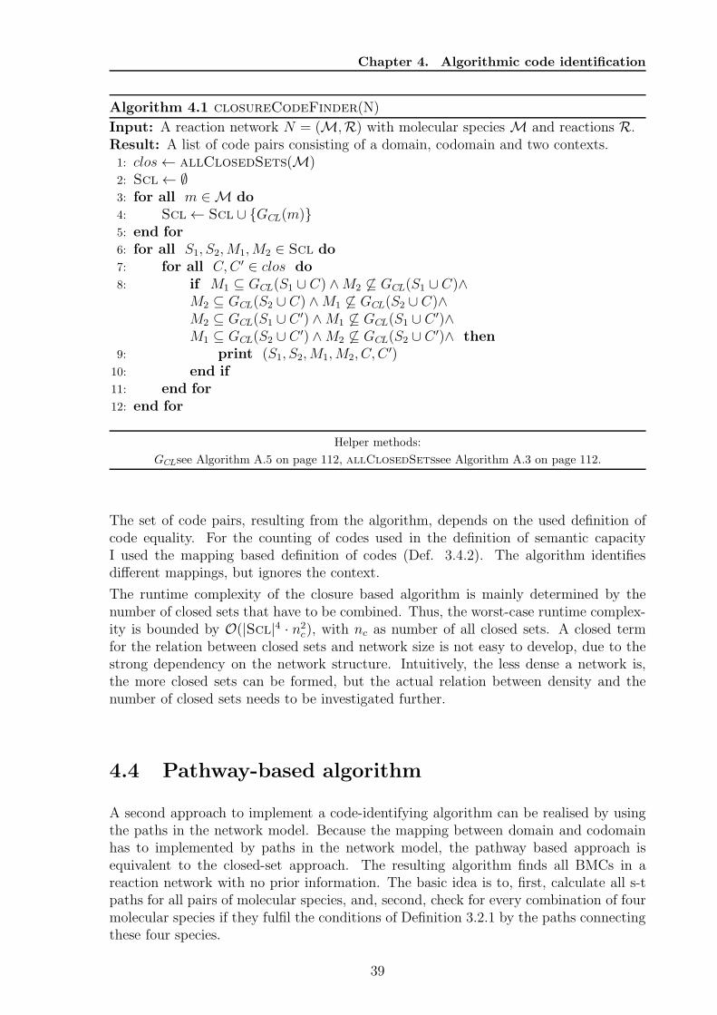
Chapter 4. Algorithmic code identification
Algorithm 4.1 closureCodeFinder(N)
Input: A reaction network N = (M,R) with molecular speciesM and reactions R.Result: A list of code pairs consisting of a domain, codomain and two contexts.1: clos← allClosedSets(M)2: Scl← ∅3: for all m ∈M do4: Scl← Scl ∪ {GCL(m)}5: end for6: for all S1, S2,M1,M2 ∈ Scl do7: for all C,C ′ ∈ clos do8: if M1 ⊆ GCL(S1 ∪ C) ∧M2 6⊆ GCL(S1 ∪ C)∧
M2 ⊆ GCL(S2 ∪ C) ∧M1 6⊆ GCL(S2 ∪ C)∧M2 ⊆ GCL(S1 ∪ C ′) ∧M1 6⊆ GCL(S1 ∪ C ′)∧M1 ⊆ GCL(S2 ∪ C ′) ∧M2 6⊆ GCL(S2 ∪ C ′)∧ then
9: print (S1, S2,M1,M2, C, C′)
10: end if11: end for12: end for
Helper methods:
GCLsee Algorithm A.5 on page 112, allClosedSetssee Algorithm A.3 on page 112.
The set of code pairs, resulting from the algorithm, depends on the used definition ofcode equality. For the counting of codes used in the definition of semantic capacityI used the mapping based definition of codes (Def. 3.4.2). The algorithm identifiesdifferent mappings, but ignores the context.
The runtime complexity of the closure based algorithm is mainly determined by thenumber of closed sets that have to be combined. Thus, the worst-case runtime complex-ity is bounded by O(|Scl|4 · n2
c), with nc as number of all closed sets. A closed termfor the relation between closed sets and network size is not easy to develop, due to thestrong dependency on the network structure. Intuitively, the less dense a network is,the more closed sets can be formed, but the actual relation between density and thenumber of closed sets needs to be investigated further.
4.4 Pathway-based algorithm
A second approach to implement a code-identifying algorithm can be realised by usingthe paths in the network model. Because the mapping between domain and codomainhas to implemented by paths in the network model, the pathway based approach isequivalent to the closed-set approach. The resulting algorithm finds all BMCs in areaction network with no prior information. The basic idea is to, first, calculate all s-tpaths for all pairs of molecular species, and, second, check for every combination of fourmolecular species if they fulfil the conditions of Definition 3.2.1 by the paths connectingthese four species.
39
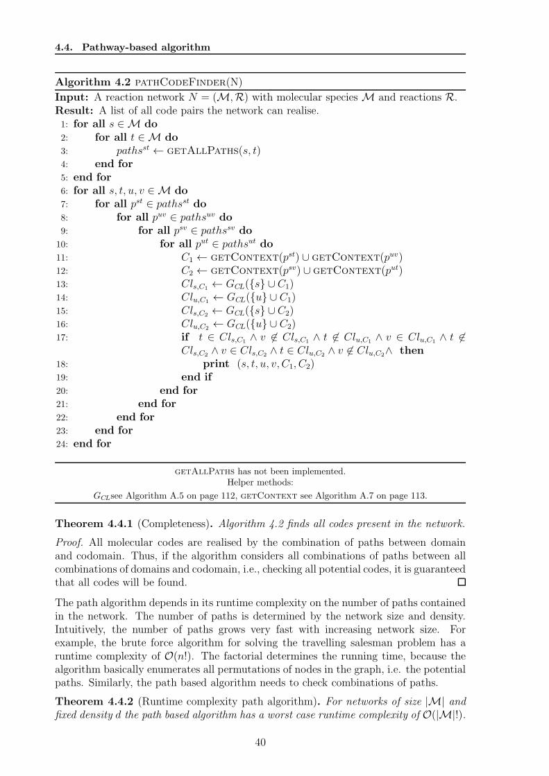
4.4. Pathway-based algorithm
Algorithm 4.2 pathCodeFinder(N)
Input: A reaction network N = (M,R) with molecular speciesM and reactions R.Result: A list of all code pairs the network can realise.1: for all s ∈M do2: for all t ∈M do3: pathsst ← getAllPaths(s, t)4: end for5: end for6: for all s, t, u, v ∈M do7: for all pst ∈ pathsst do8: for all puv ∈ pathsuv do9: for all psv ∈ pathssv do
10: for all put ∈ pathsut do11: C1 ← getContext(pst) ∪ getContext(puv)12: C2 ← getContext(psv) ∪ getContext(put)13: Cls,C1 ← GCL({s} ∪ C1)14: Clu,C1 ← GCL({u} ∪ C1)15: Cls,C2 ← GCL({s} ∪ C2)16: Clu,C2 ← GCL({u} ∪ C2)17: if t ∈ Cls,C1 ∧ v 6∈ Cls,C1 ∧ t 6∈ Clu,C1 ∧ v ∈ Clu,C1 ∧ t 6∈
Cls,C2 ∧ v ∈ Cls,C2 ∧ t ∈ Clu,C2 ∧ v 6∈ Clu,C2∧ then18: print (s, t, u, v, C1, C2)19: end if20: end for21: end for22: end for23: end for24: end for
getAllPaths has not been implemented.Helper methods:
GCLsee Algorithm A.5 on page 112, getContext see Algorithm A.7 on page 113.
Theorem 4.4.1 (Completeness). Algorithm 4.2 finds all codes present in the network.
Proof. All molecular codes are realised by the combination of paths between domainand codomain. Thus, if the algorithm considers all combinations of paths between allcombinations of domains and codomain, i.e., checking all potential codes, it is guaranteedthat all codes will be found.
The path algorithm depends in its runtime complexity on the number of paths containedin the network. The number of paths is determined by the network size and density.Intuitively, the number of paths grows very fast with increasing network size. Forexample, the brute force algorithm for solving the travelling salesman problem has aruntime complexity of O(n!). The factorial determines the running time, because thealgorithm basically enumerates all permutations of nodes in the graph, i.e. the potentialpaths. Similarly, the path based algorithm needs to check combinations of paths.
Theorem 4.4.2 (Runtime complexity path algorithm). For networks of size |M| andfixed density d the path based algorithm has a worst case runtime complexity of O(|M|!).
40
Chapter 4. Algorithmic code identification
I will proof this theorem by applying results from the analysis of random networkspublished by Roberts and Kroese [66]. The authors basically presented an estimationon the number of s-t paths in random networks, verified by a Monte-Carlo samplingtechnique. I will use their result as estimate for the number of paths here.
Proof. Given a reaction network N = (M,R) of size |M| and density d = |R|(|M|·|M|−1)
the number of s-t paths can be estimated by
Z|M|;d = K(|M|) · d|M|−1+δ(|M|,d),
where K(n) =∑n−2
k=0(n−2)!
k!, and δ(n, d) = 3.32
n− 5.16
dn[66]. The algorithm checks the BMC
condition for all combinations of four molecular species s, t, u, v ∈ M by combiningall paths for the combinations (s, t), (u, v), (s, v), (u, t). For each combination of four
species,(|M|4
), Z|M|;d paths have to be checked at maximum leading to O(Z|M|;d
4
·(|M|4
)).
So the resulting algorithm solves the problem of identifying all binary molecular codesin polynomial time in the number of paths. Over network size, with a fixed density d,the factorial terms in K(|M|) dominate leading to O(|M|!) as runtime complexity.
The path algorithm (Algorithm 4.2) has very large running times (Theorem 4.4.2) atlarge networks and networks with many paths. By applying a parametrisation to thealgorithm the runtime behaviour can be reduced. A straightforward parametrisationis to use only the K-shortest paths, instead of all paths, for every pair of molecularspecies as basis for the code identification. Identifying the K-shortest paths betweentwo vertices of a graph is a general problem in graph theory for which several algorithmshave already been developed [67, 68]. TheK shortest paths problem has many importantapplications for finding alternative solutions in bioinformatics, e.g. metabolic pathwayfinding [69] problems.In Algorithm 4.2 getAllPaths(s,t) is replaced by the function getKShortest-Paths(s,t,K) leading to pathCodeFinder(N,K).For getKShortestPaths(s,t,K) I use the freely available implementation1 by Martinet al.[70]. The algorithm is based on Yen’s algorithm [67] with a worst case runningtime of O(Kn(m + n log n)) to identify the K shortest paths between nodes s and t,with n as number of nodes and m as number of edges of the graph.To use the implementation by Martin a preprocessing step is needed. The reactionnetwork, which is mathematically a hypergraph, is transformed to a bipartite graph.The bipartite graph is generated by introducing a vertex for each reaction and by linkingreactants and product to this vertex. A reaction A + B → C + D is transformed to A
→ R, B → R, R → C, R → D.The graph used for the path identification then contains |M|+ |R| nodes. The numberof edges m is given by the reaction’s order and, thus, strongly depends on the networkstructure.
Theorem 4.4.3 (Runtime complexity for the K-shortest path algorithm). For networksof size |M| with fixed density d and a given K the K-shortest path based algorithm hasa worst case runtime complexity of O(|M|4K4).
Proof. As preprocessing step the K-shortest paths for all pairs of molecular species haveto be calculated on the bipartite network model with size N = |M|+ |R|. Because there
1Available at http://code.google.com/p/k-shortest-paths/
41
4.5. Implementation and runtime evaluation
exist(|M|2
)= |M|(|M|−1)
2pairs of species, the runtime complexity of the preprocessing is
O((KN(m+N logN)
|M|(|M| − 1)
2
).
Subsequently, for each combination of four species all combinations of the K paths has tobe checked for the code property. Because for each combination of two species maximumK paths exist, the second part of the algorithms takes K4 ”time steps” per combinationof four species. The second part of the algorithm is bounded by O(
(|M|4
)K4). The
runtime complexity of the complete algorithm (preprocessing + code checking) is thesum of the two terms leading to
O([
(KN(m+N logN)|M|(|M| − 1)
2)
]+
(|M|4
)K4
).
The left term grows with a polynomial of order 2, while the right term grows with a poly-
nomial of order 4 in |M|, because(|M|4
)= |M|(|M|−1)(|M|−2)(|M|−3)
4·3·2 = |M|4−6|M|3+11|M|2−6|M|24
.The polynomial of order 4 dominates the asymptotic runtime behaviour and for fixedK we get O(|M|4K4) as final asymptotic runtime.
The parametrisation bounded the factorial growth on paths and leaves a polynomial-time algorithm. The parametrised algorithm cannot find codes that use paths longerthan the K shortest path. This can happen if many short paths exists between thepotential sign and meaning that do not fulfil the code condition. This drawback can beeliminated by choosing K large enough, which results in larger running times, in theworst case again determined by a factorial. A promising result in this respect is thatmolecular codes are maintained to be efficient, i.e., their costs are minimised [23], sothat it seems reasonable to assume that efficient molecular codes are realised by shortpaths. The parametrisation, thus, is likely not to miss the cost-optimal codes.
4.5 Implementation and runtime evaluation
The closure based and the K-shortest paths based algorithm have been implemented inJava.I compared both algorithms for their practical runtime properties on different probleminstances. As test networks I generated random reaction networks according to Algo-rithm A.2 with different size and density. Size and density have a direct effect of thenumber of closed sets and paths in the network. The more dense a network is the mores, t-paths between the species of the network exists. The number of closed sets decreaseswith growing density.The closure algorithm is very quick on networks of size 5 and needs approximately thesame amount of time for each network on average. This is a special case since thesenetwork does not have enough closed sets, where at least 10 closed sets are necessary forcode identification (cp. Lemma 3.2.1). In general, the closure algorithm performs wellon networks with higher densities (less closed sets) and worse on lower densities. Forrandom networks of size 20 the running time is already very large (> 1.7 · 105seconds ≈2days).The path algorithm shows the opposite behaviour. The more reactions are containedin a network the more paths needs to be checked, which increases the runtime. If K
42
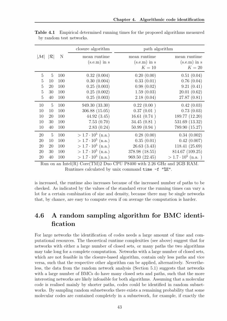
Chapter 4. Algorithmic code identification
Table 4.1 Empirical determined running times for the proposed algorithms measuredby random test networks.
closure algorithm path algorithm
|M| |R| N mean runtime(s.e.m) in s
mean runtime(s.e.m) in s
mean runtime(s.e.m) in s
K = 10 K = 20
5 5 100 0.32 (0.004) 0.20 (0.00) 0.51 (0.04)5 10 100 0.30 (0.004) 0.33 (0.01) 0.76 (0.04)5 20 100 0.25 (0.003) 0.98 (0.02) 9.21 (0.41)5 30 100 0.25 (0.002) 1.59 (0.03) 20.01 (0.62)5 40 100 0.25 (0.003) 2.18 (0.04) 27.87 (0.81)
10 5 100 949.30 (33.30) 0.22 (0.00 ) 0.42 (0.03)10 10 100 306.88 (15.05) 0.37 (0.01 ) 0.73 (0.03)10 20 100 44.92 (3.45) 16.61 (0.74 ) 189.77 (12.20)10 30 100 7.53 (0.70) 34.45 (0.81 ) 531.69 (13.32)10 40 100 2.83 (0.24) 50.99 (0.94 ) 789.90 (15.27)
20 5 100 > 1.7 · 105 (n.a.) 0.28 (0.00) 0.34 (0.002)20 10 100 > 1.7 · 105 (n.a.) 0.35 (0.01) 0.42 (0.007)20 20 100 > 1.7 · 105 (n.a.) 26.63 (3.43) 118.41 (25.69)20 30 100 > 1.7 · 105 (n.a.) 378.98 (18.55) 814.67 (109.25)20 40 100 > 1.7 · 105 (n.a.) 969.50 (22.45) > 1.7 · 105 (n.a. )
Run on an Intel(R) Core(TM)2 Duo CPU P8400 with 2.26 GHz and 2GB RAM.Runtimes calculated by unix command time -f "%E".
is increased, the runtime also increases because of the increased number of paths to bechecked. As indicated by the values of the standard error the running times can vary alot for a certain combination of size and density, because there may be single networksthat, by chance, are easy to compute even if on average the computation is harder.
4.6 A random sampling algorithm for BMC identi-
fication
For large networks the identification of codes needs a large amount of time and com-putational resources. The theoretical runtime complexities (see above) suggest that fornetworks with either a large number of closed sets, or many paths the two algorithmsmay take long for a complete computation. Networks with a large number of closed sets,which are not feasible in the closure-based algorithm, contain only less paths and viceversa, such that the respective other algorithm can be applied, alternatively. Neverthe-less, the data from the random network analysis (Section 5.1) suggests that networkswith a large number of BMCs do have many closed sets and paths, such that the moreinteresting networks are likely infeasible for both algorithms. Assuming that a molecularcode is realised mainly by shorter paths, codes could be identified in random subnet-works. By sampling random subnetworks there exists a remaining probability that somemolecular codes are contained completely in a subnetwork, for example, if exactly the
43
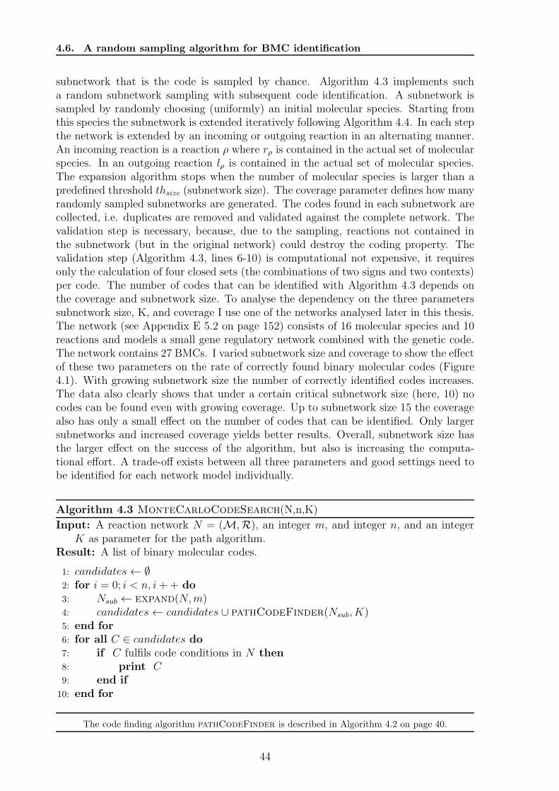
4.6. A random sampling algorithm for BMC identification
subnetwork that is the code is sampled by chance. Algorithm 4.3 implements sucha random subnetwork sampling with subsequent code identification. A subnetwork issampled by randomly choosing (uniformly) an initial molecular species. Starting fromthis species the subnetwork is extended iteratively following Algorithm 4.4. In each stepthe network is extended by an incoming or outgoing reaction in an alternating manner.An incoming reaction is a reaction ρ where rρ is contained in the actual set of molecularspecies. In an outgoing reaction lρ is contained in the actual set of molecular species.The expansion algorithm stops when the number of molecular species is larger than apredefined threshold thsize (subnetwork size). The coverage parameter defines how manyrandomly sampled subnetworks are generated. The codes found in each subnetwork arecollected, i.e. duplicates are removed and validated against the complete network. Thevalidation step is necessary, because, due to the sampling, reactions not contained inthe subnetwork (but in the original network) could destroy the coding property. Thevalidation step (Algorithm 4.3, lines 6-10) is computational not expensive, it requiresonly the calculation of four closed sets (the combinations of two signs and two contexts)per code. The number of codes that can be identified with Algorithm 4.3 depends onthe coverage and subnetwork size. To analyse the dependency on the three parameterssubnetwork size, K, and coverage I use one of the networks analysed later in this thesis.The network (see Appendix E 5.2 on page 152) consists of 16 molecular species and 10reactions and models a small gene regulatory network combined with the genetic code.The network contains 27 BMCs. I varied subnetwork size and coverage to show the effectof these two parameters on the rate of correctly found binary molecular codes (Figure4.1). With growing subnetwork size the number of correctly identified codes increases.The data also clearly shows that under a certain critical subnetwork size (here, 10) nocodes can be found even with growing coverage. Up to subnetwork size 15 the coveragealso has only a small effect on the number of codes that can be identified. Only largersubnetworks and increased coverage yields better results. Overall, subnetwork size hasthe larger effect on the success of the algorithm, but also is increasing the computa-tional effort. A trade-off exists between all three parameters and good settings need tobe identified for each network model individually.
Algorithm 4.3 MonteCarloCodeSearch(N,n,K)
Input: A reaction network N = (M,R), an integer m, and integer n, and an integerK as parameter for the path algorithm.
Result: A list of binary molecular codes.
1: candidates← ∅2: for i = 0; i < n, i++ do3: Nsub ← expand(N,m)4: candidates← candidates ∪ pathCodeFinder(Nsub, K)5: end for6: for all C ∈ candidates do7: if C fulfils code conditions in N then8: print C9: end if
10: end for
The code finding algorithm pathCodeFinder is described in Algorithm 4.2 on page 40.
44
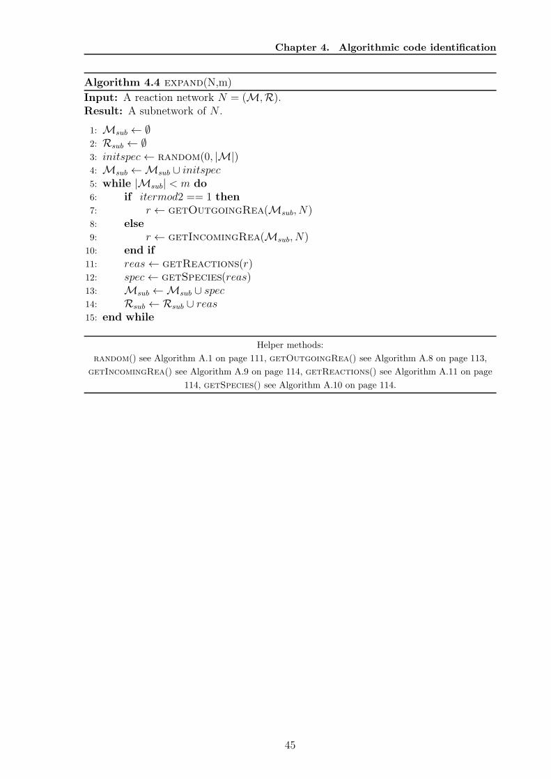
Chapter 4. Algorithmic code identification
Algorithm 4.4 expand(N,m)
Input: A reaction network N = (M,R).Result: A subnetwork of N .
1: Msub ← ∅2: Rsub ← ∅3: initspec← random(0, |M|)4: Msub ←Msub ∪ initspec5: while |Msub| < m do6: if itermod2 == 1 then7: r ← getOutgoingRea(Msub, N)8: else9: r ← getIncomingRea(Msub, N)10: end if11: reas← getReactions(r)12: spec← getSpecies(reas)13: Msub ←Msub ∪ spec14: Rsub ←Rsub ∪ reas15: end while
Helper methods:
random() see Algorithm A.1 on page 111, getOutgoingRea() see Algorithm A.8 on page 113,
getIncomingRea() see Algorithm A.9 on page 114, getReactions() see Algorithm A.11 on page
114, getSpecies() see Algorithm A.10 on page 114.
45
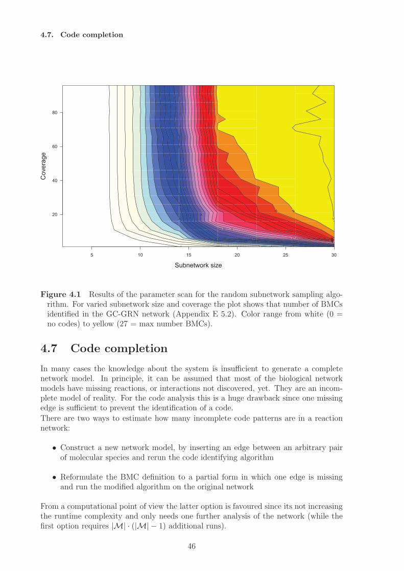
4.7. Code completion
5 10 15 20 25 30
20
40
60
80
Subnetwork size
Cov
erag
e
1 2 3 4 5 6
7
8 9
10
11
12
13
14
15 16
17 18 19 20 21 22 23 24
25
26
27
Figure 4.1 Results of the parameter scan for the random subnetwork sampling algo-rithm. For varied subnetwork size and coverage the plot shows that number of BMCsidentified in the GC-GRN network (Appendix E 5.2). Color range from white (0 =no codes) to yellow (27 = max number BMCs).
4.7 Code completion
In many cases the knowledge about the system is insufficient to generate a completenetwork model. In principle, it can be assumed that most of the biological networkmodels have missing reactions, or interactions not discovered, yet. They are an incom-plete model of reality. For the code analysis this is a huge drawback since one missingedge is sufficient to prevent the identification of a code.
There are two ways to estimate how many incomplete code patterns are in a reactionnetwork:
• Construct a new network model, by inserting an edge between an arbitrary pairof molecular species and rerun the code identifying algorithm
• Reformulate the BMC definition to a partial form in which one edge is missingand run the modified algorithm on the original network
From a computational point of view the latter option is favoured since its not increasingthe runtime complexity and only needs one further analysis of the network (while thefirst option requires |M| · (|M| − 1) additional runs).
46
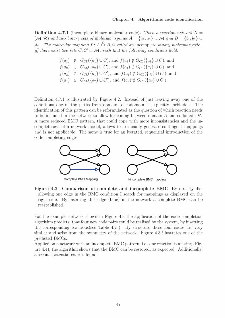
Chapter 4. Algorithmic code identification
Definition 4.7.1 (incomplete binary molecular code). Given a reaction network N =(M,R) and two binary sets of molecular species A = {a1, a2} ⊆ M and B = {b1, b2} ⊆M. The molecular mapping f : A
C�→ B is called an incomplete binary molecular code ,iff there exist two sets C,C ′ ⊆M, such that the following conditions hold:
f(a1) ∈ GCL({a1} ∪ C), and f(a2) /∈ GCL({a1} ∪ C), and
f(a2) ∈ GCL({a2} ∪ C), and f(a1) /∈ GCL({a2} ∪ C), and
f(a2) ∈ GCL({a1} ∪ C ′), and f(a1) /∈ GCL({a1} ∪ C ′), and
f(a1) ∈ GCL({a2} ∪ C ′), and f(a2) /∈ GCL({a2} ∪ C ′).
Definition 4.7.1 is illustrated by Figure 4.2. Instead of just leaving away one of theconditions one of the paths from domain to codomain is explicitly forbidden. Theidentification of this pattern can be reformulated as the question of which reaction needsto be included in the network to allow for coding between domain A and codomain B.A more reduced BMC pattern, that could cope with more inconsistencies and the in-completeness of a network model, allows to artificially generate contingent mappingsand is not applicable. The same is true for an iterated, sequential introduction of thecode completing edges.
Complete BMC Mapping 1-incomplete BMC mapping
Figure 4.2 Comparison of complete and incomplete BMC. By directly dis-allowing one edge in the BMC condition I search for mappings as displayed on theright side. By inserting this edge (blue) in the network a complete BMC can bereestablished.
For the example network shown in Figure 4.3 the application of the code completionalgorithm predicts, that four new code pairs could be realised by the system, by insertingthe corresponding reactions(see Table 4.2 ). By structure these four codes are verysimilar and arise from the symmetry of the network. Figure 4.3 illustrates one of thepredicted BMCs.Applied on a network with an incomplete BMC pattern, i.e. one reaction is missing (Fig-ure 4.4), the algorithm shows that the BMC can be restored, as expected. Additionally,a second potential code is found.
47
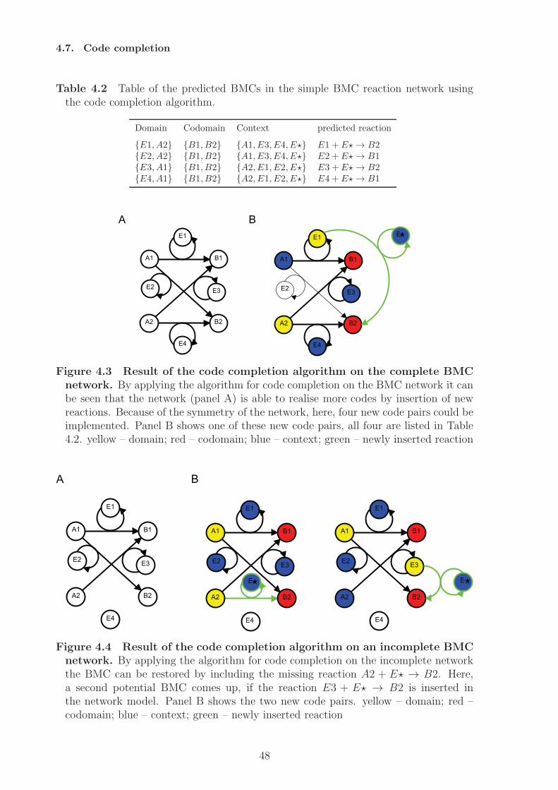
4.7. Code completion
Table 4.2 Table of the predicted BMCs in the simple BMC reaction network usingthe code completion algorithm.
Domain Codomain Context predicted reaction
{E1, A2} {B1, B2} {A1, E3, E4, E�} E1 + E�→ B2{E2, A2} {B1, B2} {A1, E3, E4, E�} E2 + E�→ B1{E3, A1} {B1, B2} {A2, E1, E2, E�} E3 + E�→ B2{E4, A1} {B1, B2} {A2, E1, E2, E�} E4 + E�→ B1
A B
A1
A2
B1
B2
E1
E2 E3
E4
A1
A2
B1
B2
E1
E2 E3
E4
E
Figure 4.3 Result of the code completion algorithm on the complete BMCnetwork. By applying the algorithm for code completion on the BMC network it canbe seen that the network (panel A) is able to realise more codes by insertion of newreactions. Because of the symmetry of the network, here, four new code pairs could beimplemented. Panel B shows one of these new code pairs, all four are listed in Table4.2. yellow – domain; red – codomain; blue – context; green – newly inserted reaction
A1
A2
B1
B2
E1
E2 E3
E4
A1
A2
B1
B2
E1
E2 E3
E4
A1
A2
B1
B2
E1
E2 E3
E4
EE
A B
Figure 4.4 Result of the code completion algorithm on an incomplete BMCnetwork. By applying the algorithm for code completion on the incomplete networkthe BMC can be restored by including the missing reaction A2 + E� → B2. Here,a second potential BMC comes up, if the reaction E3 + E� → B2 is inserted inthe network model. Panel B shows the two new code pairs. yellow – domain; red –codomain; blue – context; green – newly inserted reaction
48
Chapter 5
Results of the algorithmic codeanalysis of various systems
Parts and first ideas of this chapter have been published in [60] and [32].In this chapter I present the algorithmic, code based analysis of a number differentnetworks, among them random reaction networks, combustion chemistries, gene trans-lation, gene regulation, protein assembly networks and an artificial chemistry. Finally,I will present the results on two large scale biological networks and discuss problems inthe analysis that can arise using the algorithmic code identification on database derivednetworks.
5.1 Random networks
I analysed random networks for their capability to realize binary molecular codes. Thestatic definition of molecular codes results in a combination of molecular species andpaths and thus the probability, that such a pattern occurs by chance, is larger than zero.The probability depends on three factors:
• network size – if the network is not large enough, the code pattern can not begenerated
• network density – if there does not exist enough connection/reactions between themolecular species the paths between domain and codomain can not established
• reaction order – to establish a molecular context reactions of (at least) order 2 areneeded. A network with only spontaneous reactions can not have molecular codes
For this study I generated random networks of varying size and density, but with a fixedreaction order. Random reactions are of the form A + B → C, i.e. each reaction is”regulated” in the sense that a second molecular species is necessary for the reaction.Algorithm A.2 describes the network generation. In principle, it is possible to vary alsothe distribution of reaction orders in the networks. For this study I am primarily inter-ested in size and density, because these two parameters directly influence the numberof paths and closed sets (cf. the formulation of the algorithms, Chapter 4). Reactionorder plays, therefore, only a minor role and is kept constant. For each combinationof network size and density I generated 1000 random networks and applied the codeidentifying algorithm.
49
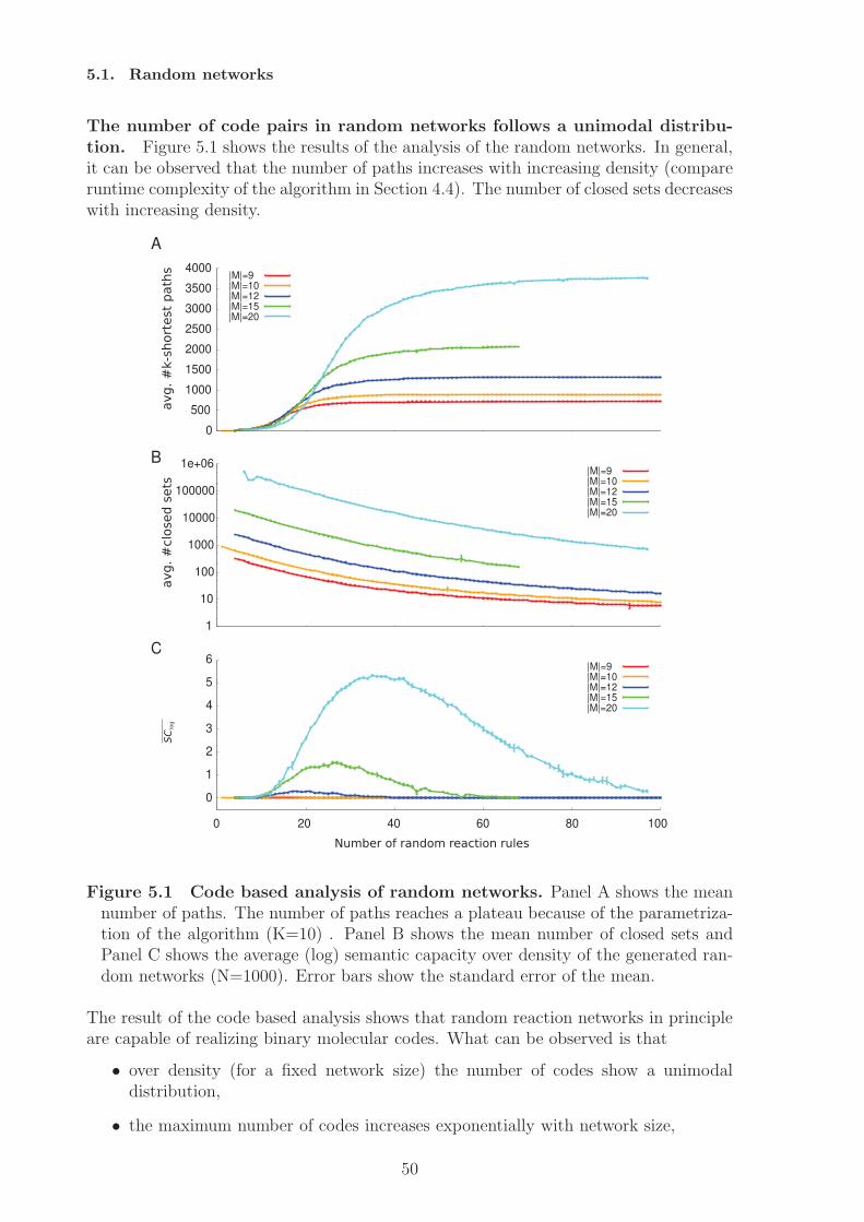
5.1. Random networks
The number of code pairs in random networks follows a unimodal distribu-tion. Figure 5.1 shows the results of the analysis of the random networks. In general,it can be observed that the number of paths increases with increasing density (compareruntime complexity of the algorithm in Section 4.4). The number of closed sets decreaseswith increasing density.
0
1
2
3
4
5
6
0 20 40 60 80 100
C|M|=9|M|=10|M|=12|M|=15|M|=20
1
10
100
1000
10000
100000
1e+06B|M|=9|M|=10|M|=12|M|=15|M|=20
0
500
1000
1500
2000
2500
3000
3500
4000
A
|M|=9|M|=10|M|=12|M|=15|M|=20
Figure 5.1 Code based analysis of random networks. Panel A shows the meannumber of paths. The number of paths reaches a plateau because of the parametriza-tion of the algorithm (K=10) . Panel B shows the mean number of closed sets andPanel C shows the average (log) semantic capacity over density of the generated ran-dom networks (N=1000). Error bars show the standard error of the mean.
The result of the code based analysis shows that random reaction networks in principleare capable of realizing binary molecular codes. What can be observed is that
• over density (for a fixed network size) the number of codes show a unimodaldistribution,
• the maximum number of codes increases exponentially with network size,
50
Chapter 5. Results of the algorithmic code analysis of various systems
• the position of the mean (and thus the position of the optimal interval) shiftslinearly to larger densities with network size.
The extend of the distribution (Figure 5.1C) gives an optimal interval for random codegeneration, i.e., random networks with this size and a density lying in the interval arevery likely to have codes by chance.
Statistical (null-)model. For the development of a null-model that allows the pre-diction of the semantic capacity also for combinations of network sizes and densitiesthat have not been generated as random networks I developed a statistical model.To obtain such a statistical model I assume that the average number of code pairs followsan unknown probability distribution and fit a statistical model on the data.In general, the mean number xs of BMCs over the network density for a fixed network sizeis modelled as random variable X ∼ D. X follows an unknown probability distributionD.As candidate distributions I chose the normal (N (µ, σ2)), the log - normal (lnN (µ, σ2))and a gamma distribution (Γ(k, θ))1. All show a unimodal behavior for certain param-eter combinations, but behave differently in their properties (e.g. skewness). All threedistributions are commonly used for statistical purposes.My approach here will be to estimate the candidate distribution’s parameters from thedata by using the empirical mean µ and variance σ2. I calculate the goodness of fit toselect the most suitable model.In the following I show how the candidate distribution’s parameters are related to theempirical mean and variance.
Normal distribution The normal distribution’s probability density function is givenby
fN (x) =1√2πσ2
e−(x−µ)2
2σ2 .
The normal distribution’s mean and variance are given by µ and σ2, such that for theestimate the empirical values can be used directly.
Log-normal distribution The log-normal distribution is a probability distributionwhose logarithm is normally distributed. The probability density function is given by
flnN (x) =1
x√2πσ2
e−(lnx−µ)2
2σ2 .
The mean of the distribution is given by eµ+σ2
2 , while the variance is given by (eσ2 −
1)e2µ+σ2. To calculate the distribution’s parameters from the empirical mean and vari-
ance I will solve the following system of equations for µ and σ2:
µ = eµ+σ2
2 (5.1)
σ2 = (eσ2 − 1)e2µ+σ2
. (5.2)
I solve Eq. (5.1) for µ.
1Not to be confused with the gamma function, which is defined via factorials, but is used to calculatethe gamma distribution.
51
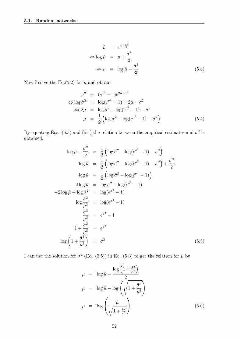
5.1. Random networks
µ = eµ+σ2
2
⇔ log µ = µ+σ2
2
⇔ µ = log µ− σ2
2(5.3)
Now I solve the Eq.(5.2) for µ and obtain
σ2 = (eσ2 − 1)e2µ+σ2
⇔ log σ2 = log(eσ2 − 1) + 2µ+ σ2
⇔ 2µ = log σ2 − log(eσ2 − 1)− σ2
µ =1
2
(log σ2 − log(eσ
2 − 1)− σ2)
(5.4)
By equating Eqs. (5.3) and (5.4) the relation between the empirical estimates and σ2 isobtained.
log µ− σ2
2=
1
2
(log σ2 − log(eσ
2 − 1)− σ2)
log µ =1
2
(log σ2 − log(eσ
2 − 1)− σ2)+
σ2
2
log µ =1
2
(log σ2 − log(eσ
2 − 1))
2 log µ = log σ2 − log(eσ2 − 1)
−2 log µ+ log σ2 = log(eσ2 − 1)
logσ2
µ2= log(eσ
2 − 1)
σ2
µ2= eσ
2 − 1
1 +σ2
µ2= eσ
2
log
(1 +
σ2
µ2
)= σ2 (5.5)
I can use the solution for σ2 (Eq. (5.5)) in Eq. (5.3) to get the relation for µ by
µ = log µ−log(1 + σ2
µ2
)
2
µ = log µ− log
(√1 +
σ2
µ2
)
µ = log
µ√
1 + σ2
µ2
(5.6)
52
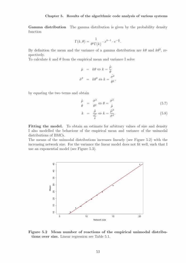
Chapter 5. Results of the algorithmic code analysis of various systems
Gamma distribution The gamma distribution is given by the probability densityfunction
Γ(k, θ) =1
θkΓ(k)· xk−1 · e−x
θ .
By definition the mean and the variance of a gamma distribution are kθ and kθ2, re-spectively.To calculate k and θ from the empirical mean and variance I solve
μ = kθ ⇔ k =μ
θ
σ2 = kθ2 ⇔ k =σ2
θ2,
by equating the two terms and obtain
μ
θ=
σ2
θ2⇔ θ =
σ2
μ(5.7)
k =μσ2
μ
⇔ k =μ2
σ2. (5.8)
Fitting the model. To obtain an estimate for arbitrary values of size and densityI also modelled the behaviour of the empirical mean and variance of the unimodaldistributions of BMCs.The means of the unimodal distributions increases linearly (see Figure 5.2) with theincreasing network size. For the variance the linear model does not fit well, such that Iuse an exponential model (see Figure 5.3).
5 10 15 20
1015
2025
3035
4045
Network size
Mea
n
Figure 5.2 Mean number of reactions of the empirical unimodal distribu-tions over size. Linear regression see Table 5.1.
53
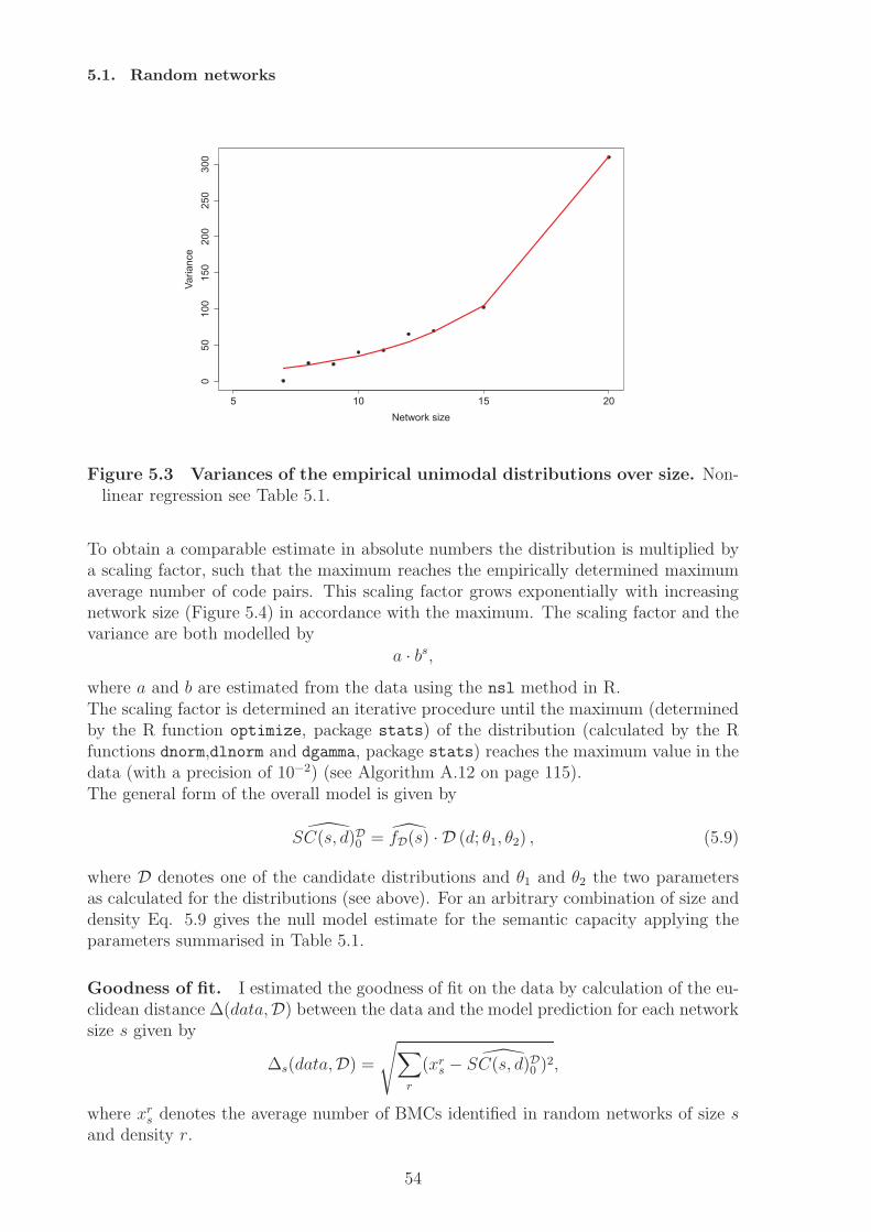
5.1. Random networks
5 10 15 20
050
100
150
200
250
300
Network size
Varia
nce
Figure 5.3 Variances of the empirical unimodal distributions over size. Non-linear regression see Table 5.1.
To obtain a comparable estimate in absolute numbers the distribution is multiplied bya scaling factor, such that the maximum reaches the empirically determined maximumaverage number of code pairs. This scaling factor grows exponentially with increasingnetwork size (Figure 5.4) in accordance with the maximum. The scaling factor and thevariance are both modelled by
a · bs,where a and b are estimated from the data using the nsl method in R.The scaling factor is determined an iterative procedure until the maximum (determinedby the R function optimize, package stats) of the distribution (calculated by the Rfunctions dnorm,dlnorm and dgamma, package stats) reaches the maximum value in thedata (with a precision of 10−2) (see Algorithm A.12 on page 115).The general form of the overall model is given by
SC(s, d)D0 = fD(s) · D (d; θ1, θ2) , (5.9)
where D denotes one of the candidate distributions and θ1 and θ2 the two parametersas calculated for the distributions (see above). For an arbitrary combination of size anddensity Eq. 5.9 gives the null model estimate for the semantic capacity applying theparameters summarised in Table 5.1.
Goodness of fit. I estimated the goodness of fit on the data by calculation of the eu-clidean distance Δ(data,D) between the data and the model prediction for each networksize s given by
Δs(data,D) =√∑
r
(xrs − SC(s, d)D0 )
2,
where xrs denotes the average number of BMCs identified in random networks of size s
and density r.
54
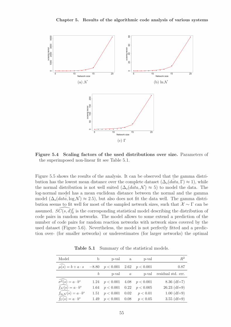
Chapter 5. Results of the algorithmic code analysis of various systems
5 10 15 20
010
0020
0030
0040
00
Network size
Sca
ling
fact
or
(a) N
5 10 15 20
020
4060
80
Network size
Sca
ling
fact
or
(b) lnN
5 10 15 20
050
100
150
200
Network size
Sca
ling
fact
or
(c) Γ
Figure 5.4 Scaling factors of the used distributions over size. Parameters ofthe superimposed non-linear fit see Table 5.1.
Figure 5.5 shows the results of the analysis. It can be observed that the gamma distri-bution has the lowest mean distance over the complete dataset ( ¯Δs(data,Γ) ≈ 1), whilethe normal distribution is not well suited ( ¯Δs(data,N ) ≈ 5) to model the data. Thelog-normal model has a mean euclidean distance between the normal and the gammamodel ( ¯Δs(data, logN ) ≈ 2.5), but also does not fit the data well. The gamma distri-bution seems to fit well for most of the sampled network sizes, such that X ∼ Γ can be
assumed. SC(s, d)Γ0 is the corresponding statistical model describing the distribution ofcode pairs in random networks. The model allows to some extend a prediction of thenumber of code pairs for random reaction networks with network sizes covered by theused dataset (Figure 5.6). Nevertheless, the model is not perfectly fitted and a predic-tion over- (for smaller networks) or underestimates (for larger networks) the optimal
Table 5.1 Summary of the statistical models.
Model b p-val a p-val R2
μ(s) = b+ a · s −8.80 p < 0.001 2.62 p < 0.001 0.87
b p-val a p-val residual std. err.
σ2(s) = a · bs 1.24 p < 0.001 4.08 p < 0.001 8.36 (df=7)
fN (s) = a · bs 1.64 p < 0.001 0.22 p < 0.005 26.23 (df=9)flnN (s) = a · bs 1.51 p < 0.001 0.02 p < 0.01 1.00 (df=9)
fΓ(s) = a · bs 1.49 p < 0.001 0.08 p < 0.05 3.55 (df=9)
55
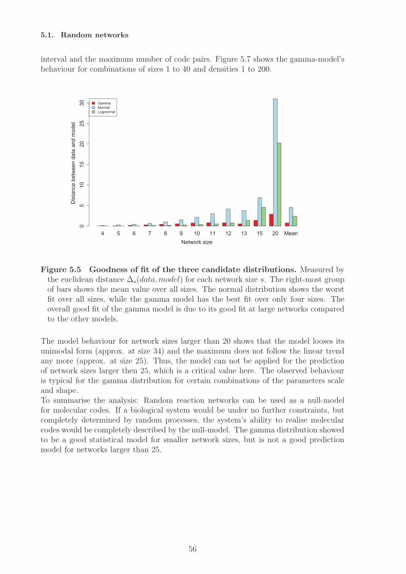
5.1. Random networks
interval and the maximum number of code pairs. Figure 5.7 shows the gamma-model’sbehaviour for combinations of sizes 1 to 40 and densities 1 to 200.
4 5 6 7 8 9 10 11 12 13 15 20 MeanNetwork size
Dis
tanc
e be
twee
n da
ta a
nd m
odel
05
1015
2025
30 GammaNormalLognormal
Figure 5.5 Goodness of fit of the three candidate distributions. Measured bythe euclidean distance Δs(data,model) for each network size s. The right-most groupof bars shows the mean value over all sizes. The normal distribution shows the worstfit over all sizes, while the gamma model has the best fit over only four sizes. Theoverall good fit of the gamma model is due to its good fit at large networks comparedto the other models.
The model behaviour for network sizes larger than 20 shows that the model looses itsunimodal form (approx. at size 34) and the maximum does not follow the linear trendany more (approx. at size 25). Thus, the model can not be applied for the predictionof network sizes larger then 25, which is a critical value here. The observed behaviouris typical for the gamma distribution for certain combinations of the parameters scaleand shape.To summarise the analysis: Random reaction networks can be used as a null-modelfor molecular codes. If a biological system would be under no further constraints, butcompletely determined by random processes, the system’s ability to realise molecularcodes would be completely described by the null-model. The gamma distribution showedto be a good statistical model for smaller network sizes, but is not a good predictionmodel for networks larger than 25.
56
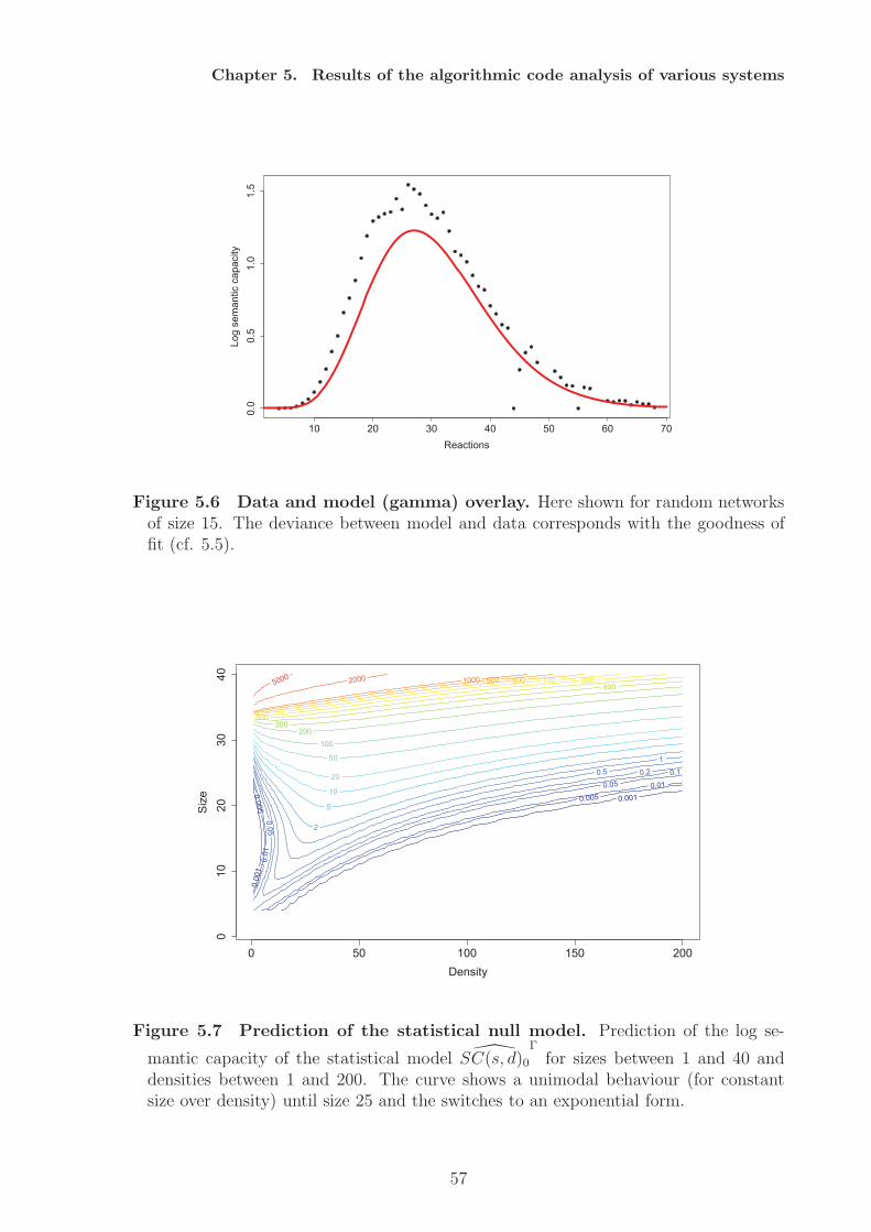
Chapter 5. Results of the algorithmic code analysis of various systems
10 20 30 40 50 60 70
0.0
0.5
1.0
1.5
Reactions
Log
sem
antic
cap
acity
Figure 5.6 Data and model (gamma) overlay. Here shown for random networksof size 15. The deviance between model and data corresponds with the goodness offit (cf. 5.5).
Density
Siz
e
0.0
01
0.001
0.005
0.005
0.0
1
0.01 0.05
0.05
0.1 0.2 0.5 1
2
5
10
20
50
100 200
300
400
500
600 700 800 900 1000 2000 5000
0 50 100 150 200
010
2030
40
Figure 5.7 Prediction of the statistical null model. Prediction of the log se-
mantic capacity of the statistical model SC(s, d)0Γ
for sizes between 1 and 40 anddensities between 1 and 200. The curve shows a unimodal behaviour (for constantsize over density) until size 25 and the switches to an exponential form.
57
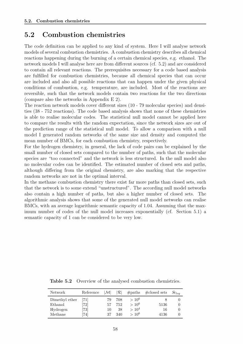
5.2. Combustion chemistries
5.2 Combustion chemistries
The code definition can be applied to any kind of system. Here I will analyse networkmodels of several combustion chemistries. A combustion chemistry describes all chemicalreactions happening during the burning of a certain chemical species, e.g. ethanol. Thenetwork models I will analyse here are from different sources (cf. 5.2) and are consideredto contain all relevant reactions. The prerequisites necessary for a code based analysisare fulfilled for combustion chemistries, because all chemical species that can occurare included and also all possible reactions that can happen under the given physicalconditions of combustion, e.g. temperature, are included. Most of the reactions arereversible, such that the network models contain two reactions for the two directions(compare also the networks in Appendix E 2).The reaction network models cover different sizes (10 - 79 molecular species) and densi-ties (38 - 752 reactions). The code based analysis shows that none of these chemistriesis able to realise molecular codes. The statistical null model cannot be applied hereto compare the results with the random expectation, since the network sizes are out ofthe prediction range of the statistical null model. To allow a comparison with a nullmodel I generated random networks of the same size and density and computed themean number of BMCs, for each combustion chemistry, respectively.For the hydrogen chemistry, in general, the lack of code pairs can be explained by thesmall number of closed sets compared to the number of paths, such that the molecularspecies are “too connected” and the network is less structured. In the null model alsono molecular codes can be identified. The estimated number of closed sets and paths,although differing from the original chemistry, are also marking that the respectiverandom networks are not in the optimal interval.In the methane combustion chemistry there exist far more paths than closed sets, suchthat the network is to some extend “unstructured”. The according null model networksalso contain a high number of paths, but also a higher number of closed sets. Thealgorithmic analysis shows that some of the generated null model networks can realiseBMCs, with an average logarithmic semantic capacity of 1.04. Assuming that the max-imum number of codes of the null model increases exponentially (cf. Section 5.1) asemantic capacity of 1 can be considered to be very low.
Table 5.2 Overview of the analysed combustion chemistries.
Network Reference |M| |R| #paths #closed sets Sclog
Dimethyl ether [71] 79 708 > 106 8 0Ethanol [72] 57 752 > 106 5136 0Hydrogen [73] 10 38 > 104 16 0Methane [74] 37 340 > 106 4136 0
58
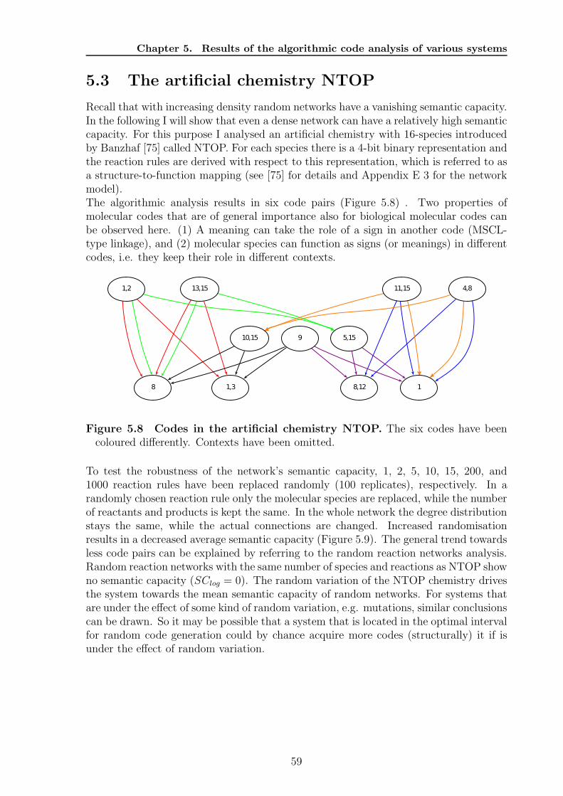
Chapter 5. Results of the algorithmic code analysis of various systems
5.3 The artificial chemistry NTOP
Recall that with increasing density random networks have a vanishing semantic capacity.In the following I will show that even a dense network can have a relatively high semanticcapacity. For this purpose I analysed an artificial chemistry with 16-species introducedby Banzhaf [75] called NTOP. For each species there is a 4-bit binary representation andthe reaction rules are derived with respect to this representation, which is referred to asa structure-to-function mapping (see [75] for details and Appendix E 3 for the networkmodel).The algorithmic analysis results in six code pairs (Figure 5.8) . Two properties ofmolecular codes that are of general importance also for biological molecular codes canbe observed here. (1) A meaning can take the role of a sign in another code (MSCL-type linkage), and (2) molecular species can function as signs (or meanings) in differentcodes, i.e. they keep their role in different contexts.
Figure 5.8 Codes in the artificial chemistry NTOP. The six codes have beencoloured differently. Contexts have been omitted.
To test the robustness of the network’s semantic capacity, 1, 2, 5, 10, 15, 200, and1000 reaction rules have been replaced randomly (100 replicates), respectively. In arandomly chosen reaction rule only the molecular species are replaced, while the numberof reactants and products is kept the same. In the whole network the degree distributionstays the same, while the actual connections are changed. Increased randomisationresults in a decreased average semantic capacity (Figure 5.9). The general trend towardsless code pairs can be explained by referring to the random reaction networks analysis.Random reaction networks with the same number of species and reactions as NTOP showno semantic capacity (SClog = 0). The random variation of the NTOP chemistry drivesthe system towards the mean semantic capacity of random networks. For systems thatare under the effect of some kind of random variation, e.g. mutations, similar conclusionscan be drawn. So it may be possible that a system that is located in the optimal intervalfor random code generation could by chance acquire more codes (structurally) it if isunder the effect of random variation.
59
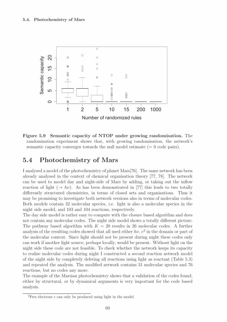
5.4. Photochemistry of Mars
1 2 5 10 15 200 1000
05
1015
20
Number of randomized rules
Sem
antic
cap
acity
Figure 5.9 Semantic capacity of NTOP under growing randomisation. Therandomisation experiment shows that, with growing randomisation, the network’ssemantic capacity converges towards the null model estimate (= 0 code pairs).
5.4 Photochemistry of Mars
I analysed a model of the photochemistry of planet Mars[76]. The same network has beenalready analysed in the context of chemical organisation theory [77, 78]. The networkcan be used to model day and night-side of Mars by adding, or taking out the inflowreaction of light (→ hν). As has been demonstrated in [77] this leads to two totallydifferently structured chemistries, in terms of closed sets and organisations. Thus itmay be promising to investigate both network versions also in terms of molecular codes.Both models contain 32 molecular species, i.e. light is also a molecular species in thenight side model, and 103 and 104 reactions, respectively.The day side model is rather easy to compute with the closure based algorithm and doesnot contain any molecular codes. The night side model shows a totally different picture.The pathway based algorithm with K = 20 results in 26 molecular codes. A furtheranalysis of the resulting codes showed that all used either hν, e2 in the domain or part ofthe molecular context. Since light should not be present during night these codes onlycan work if another light source, perhaps locally, would be present. Without light on thenight side these code are not feasible. To check whether the network keeps its capacityto realise molecular codes during night I constructed a second reaction network modelof the night side by completely deleting all reactions using light as reactant (Table 5.3)and repeated the analysis. The modified network contains 31 molecular species and 76reactions, but no codes any more.The example of the Marsian photochemistry shows that a validation of the codes found,either by structural, or by dynamical arguments is very important for the code basedanalysis.
2Free electrons e can only be produced using light in the model.
60
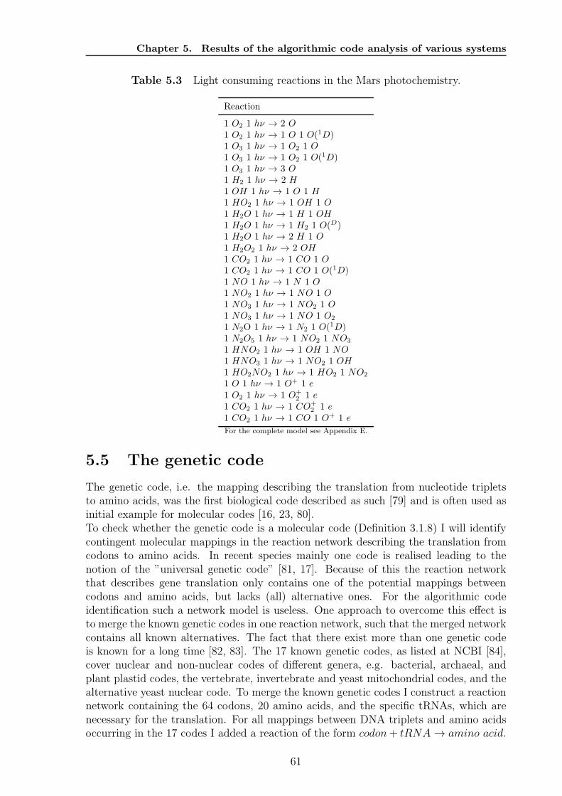
Chapter 5. Results of the algorithmic code analysis of various systems
Table 5.3 Light consuming reactions in the Mars photochemistry.
Reaction
1 O2 1 hν → 2 O
1 O2 1 hν → 1 O 1 O(1D)1 O3 1 hν → 1 O2 1 O
1 O3 1 hν → 1 O2 1 O(1D)1 O3 1 hν → 3 O
1 H2 1 hν → 2 H
1 OH 1 hν → 1 O 1 H
1 HO2 1 hν → 1 OH 1 O
1 H2O 1 hν → 1 H 1 OH
1 H2O 1 hν → 1 H2 1 O(D)1 H2O 1 hν → 2 H 1 O
1 H2O2 1 hν → 2 OH
1 CO2 1 hν → 1 CO 1 O
1 CO2 1 hν → 1 CO 1 O(1D)1 NO 1 hν → 1 N 1 O
1 NO2 1 hν → 1 NO 1 O
1 NO3 1 hν → 1 NO2 1 O
1 NO3 1 hν → 1 NO 1 O2
1 N2O 1 hν → 1 N2 1 O(1D)1 N2O5 1 hν → 1 NO2 1 NO3
1 HNO2 1 hν → 1 OH 1 NO
1 HNO3 1 hν → 1 NO2 1 OH
1 HO2NO2 1 hν → 1 HO2 1 NO2
1 O 1 hν → 1 O+ 1 e
1 O2 1 hν → 1 O+2 1 e
1 CO2 1 hν → 1 CO+2 1 e
1 CO2 1 hν → 1 CO 1 O+ 1 e
For the complete model see Appendix E.
5.5 The genetic code
The genetic code, i.e. the mapping describing the translation from nucleotide tripletsto amino acids, was the first biological code described as such [79] and is often used asinitial example for molecular codes [16, 23, 80].To check whether the genetic code is a molecular code (Definition 3.1.8) I will identifycontingent molecular mappings in the reaction network describing the translation fromcodons to amino acids. In recent species mainly one code is realised leading to thenotion of the ”universal genetic code” [81, 17]. Because of this the reaction networkthat describes gene translation only contains one of the potential mappings betweencodons and amino acids, but lacks (all) alternative ones. For the algorithmic codeidentification such a network model is useless. One approach to overcome this effect isto merge the known genetic codes in one reaction network, such that the merged networkcontains all known alternatives. The fact that there exist more than one genetic codeis known for a long time [82, 83]. The 17 known genetic codes, as listed at NCBI [84],cover nuclear and non-nuclear codes of different genera, e.g. bacterial, archaeal, andplant plastid codes, the vertebrate, invertebrate and yeast mitochondrial codes, and thealternative yeast nuclear code. To merge the known genetic codes I construct a reactionnetwork containing the 64 codons, 20 amino acids, and the specific tRNAs, which arenecessary for the translation. For all mappings between DNA triplets and amino acidsoccurring in the 17 codes I added a reaction of the form codon+ tRNA→ amino acid.
61
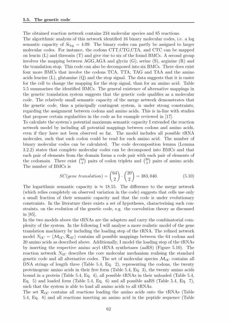
5.5. The genetic code
The obtained reaction network contains 234 molecular species and 85 reactions.The algorithmic analysis of this network identified 16 binary molecular codes, i.e. a logsemantic capacity of Sclog = 4.09. The binary codes can partly be assigned to largermolecular codes. For instance, the codons CTT,CTG,CTA, and CTC can be mappedon leucin (L) and threonin (T) and give rise to six of the found BMCs. A second groupinvolves the mapping between AGG,AGA and glycin (G), serine (S), arginine (R) andthe translation stop. This code can also be decomposed into six BMCs. There does existfour more BMCs that involve the codons TCA, TTA, TAG and TAA and the aminoacids leucine (L), glutamine (Q) and the stop signal. The data suggests that it is easierfor the cell to change the mapping for the stop signal, than for an amino acid. Table5.5 summarises the identified BMCs. The general existence of alternative mappings inthe genetic translation system suggests that the genetic code qualifies as a molecularcode. The relatively small semantic capacity of the merge network demonstrates thatthe genetic code, thus a principally contingent system, is under strong constraints,regarding the assignment between codons and amino acids. This is in-line with studiesthat propose certain regularities in the code as for example reviewed in [17].To calculate the system’s potential maximum semantic capacity I extended the reactionnetwork model by including all potential mappings between codons and amino acids,even if they have not been observed so far. The model includes all possible tRNAmolecules, such that each codon could be read for each amino acid. The number ofbinary molecular codes can be calculated. The code decomposition lemma (Lemma3.2.2) states that complete molecular codes can be decomposed into BMCs and thateach pair of elements from the domain forms a code pair with each pair of elements ofthe codomain. There exist
(642
)pairs of codon triplets and
(202
)pairs of amino acids.
The number of BMCs is
SC(gene translation) =
(64
2
)·(20
2
)= 383, 040. (5.10)
The logarithmic semantic capacity is ≈ 18.55. The difference to the merge network(which relies completely on observed variation in the code) suggests that cells use onlya small fraction of their semantic capacity and that the code is under evolutionaryconstraints. In the literature there exists a set of hypotheses, characterising such con-straints, on the evolution of the genetic code, e.g. the coevolution theory as discussedin [85].In the two models above the tRNAs are the adapters and carry the combinatorial com-plexity of the system. In the following I will analyse a more realistic model of the genetranslation machinery by including the loading step of the tRNA. The refined networkmodel NGC = 〈MGC ,RGC〉 contains all possible mappings between the 64 codons and20 amino acids as described above. Additionally, I model the loading step of the tRNAsby inserting the respective amino acyl tRNA synthetases (aaRS) (Figure 5.10). Thereaction network NGC describes the core molecular mechanism realising the standardgenetic code and all alternative codes. The set of molecular species MGC contains allDNA strings of length three (Table 5.4, Eq. 2), representing the codons, the twentyproteinogenic amino acids in their free form (Table 5.4, Eq. 3), the twenty amino acidsbound in a protein (Table 5.4, Eq. 4), all possible tRNAs in their unloaded (Table 5.4,Eq. 5) and loaded form (Table 5.4, Eq. 6) and all possible aaRS (Table 5.4, Eq. 7),such that the system is able to load all amino acids to all tRNAs.The set RGC contains all reactions loading the amino acids onto the tRNAs (Table5.4, Eq. 8) and all reactions inserting an amino acid in the peptide sequence (Table
62
Chapter 5. Results of the algorithmic code analysis of various systems
Table 5.4 Definition of the gene translation chemistry with synthetases.
Eq. Definition Description
1 MGC = Codons ∪ AAfree ∪ AAprot ∪ aaRS ∪tRNAfree ∪ tRNAloaded
Definition of the molecular species in thenetwork
2 Codons = {A,C,G,T}3= {AAA,AAC, . . . ,TTT}
Set representing the 64 codons of the geneticcode
3 AAfree ={Alafree,Argfree,Aspfree, . . . ,Tryfree}
Amino acids that are not used in a protein
4 AAprot ={Alaprot,Argprot,Aspprot, . . . ,Tryprot}
Amino acids that have been used in a proteinduring gene translation
5 tRNAfree = {tRNAn|n ∈ Codons} Unloaded tRNAs specific for codon n
6 tRNAloaded = {tRNAn,a|n ∈ Codons, a ∈AAfree}
tRNAs specific for codon n that have beenloaded with amino acid a
7 aaRS = {Synn,a|n ∈ Codons, a ∈ AAfree} Amino acyl-tRNA-synthetases that arespecific for amino acid a and codon n
8 RGC = {tRNAn + a+ Synn,a → tRNAa,n +
Synn,a | n ∈ Codons, a ∈ AAfree}∪Loading of the tRNA by suitable synthetase
9 {n+ tRNAa,n → n+ tRNAn + a | n ∈Codons, a ∈ AAprot}
Translation step, i.e., the incorporation of anamino acid into a growing protein
5.4, Eq. 9). Figure 5.10A displays a subnetwork with two codons (GGA, AGU), twoamino acids (Gly, Ser) and the respective other elements of the network (tRNA andsynthetases). Analysing this subnetwork allows to assess the whole network’s semanticcapacity. Table 5.6 shows the four molecular code pairs contained in the subsystem, therespective molecular contexts are listed in Table 5.7. The core code analysis of thesenetworks reveals that each single code is only a core code of itself (reflexivity), but nevera core code of any other code. In other words, the four codes are not generated by oneof the other codes, but stand on their own. The identified code pairs (Table 5.6) showthat not only codons can be signs, but also the unloaded tRNAs can function as signs.These additional signs increase the number of code pairs in a combinatoric manner. The”new” codes differ structurally in their molecular context. While, classically, the codonsare mapped to the set of amino acids using the loaded tRNAs as context, the new signs,i.e. unloaded tRNAs, are mapped to the set of amino acids by using a molecular contextthat consists of the free amino acid loaded to the free tRNA, the synthetase performingthe loading step, and the codon that needs to be recognised by the tRNA. The numberof code pairs in this system can be calculated by
CPGC =
[(ns
2
)− ns
2
]·(nm
2
), (5.11)
with ns as number of signs and nm as number of meanings (amino acids). For the fullgene translation system the number of signs is ns = c + t, with c as number of codonsand t as number of unloaded tRNAs. Because there is always one pair of one tRNA andone codon belonging together that can not be combined as signs in a BMC, we have tosubtract the number of such pairs ns/2 from the amount of all combinations.The analysis of the whole network (NGC), describing all potential genetic codes with 64codons and 20 amino acids, results in 1, 532, 160 binary code pairs, i.e. Sclog(NGC) ≈20.55. This is a different result than for the less detailed model, as calculated by Eq.(5.10). The extension of the model by aaRS, unloaded tRNAs, and unloaded aminoacids increases the semantic capacity.
63
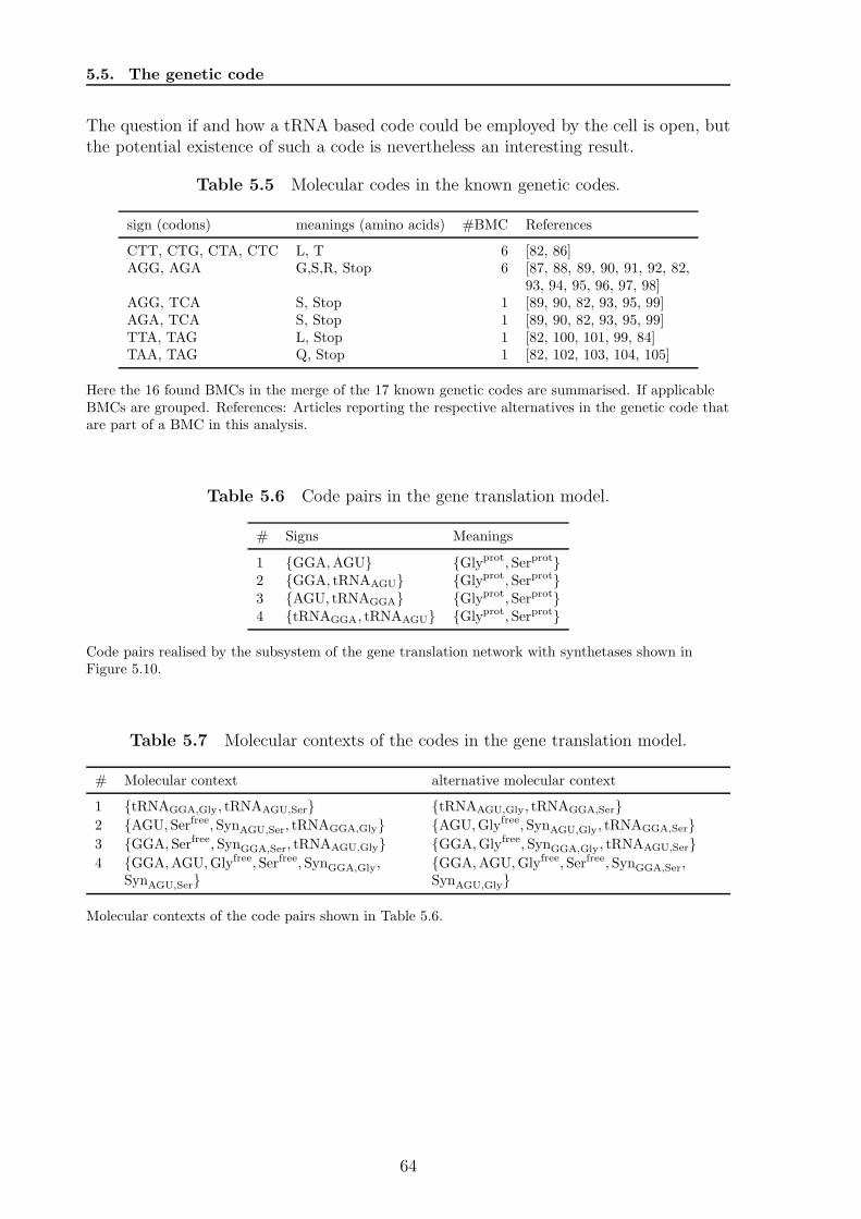
5.5. The genetic code
The question if and how a tRNA based code could be employed by the cell is open, butthe potential existence of such a code is nevertheless an interesting result.
Table 5.5 Molecular codes in the known genetic codes.
sign (codons) meanings (amino acids) #BMC References
CTT, CTG, CTA, CTC L, T 6 [82, 86]AGG, AGA G,S,R, Stop 6 [87, 88, 89, 90, 91, 92, 82,
93, 94, 95, 96, 97, 98]AGG, TCA S, Stop 1 [89, 90, 82, 93, 95, 99]AGA, TCA S, Stop 1 [89, 90, 82, 93, 95, 99]TTA, TAG L, Stop 1 [82, 100, 101, 99, 84]TAA, TAG Q, Stop 1 [82, 102, 103, 104, 105]
Here the 16 found BMCs in the merge of the 17 known genetic codes are summarised. If applicableBMCs are grouped. References: Articles reporting the respective alternatives in the genetic code thatare part of a BMC in this analysis.
Table 5.6 Code pairs in the gene translation model.
# Signs Meanings
1 {GGA,AGU} {Glyprot, Serprot}2 {GGA, tRNAAGU} {Glyprot, Serprot}3 {AGU, tRNAGGA} {Glyprot, Serprot}4 {tRNAGGA, tRNAAGU} {Glyprot, Serprot}
Code pairs realised by the subsystem of the gene translation network with synthetases shown inFigure 5.10.
Table 5.7 Molecular contexts of the codes in the gene translation model.
# Molecular context alternative molecular context
1 {tRNAGGA,Gly, tRNAAGU,Ser} {tRNAAGU,Gly, tRNAGGA,Ser}2 {AGU, Serfree, SynAGU,Ser, tRNAGGA,Gly} {AGU,Glyfree, SynAGU,Gly, tRNAGGA,Ser}3 {GGA, Serfree, SynGGA,Ser, tRNAAGU,Gly} {GGA,Glyfree, SynGGA,Gly, tRNAAGU,Ser}4 {GGA,AGU,Glyfree, Serfree, SynGGA,Gly,
SynAGU,Ser}{GGA,AGU,Glyfree, Serfree, SynGGA,Ser,
SynAGU,Gly}
Molecular contexts of the code pairs shown in Table 5.6.
64
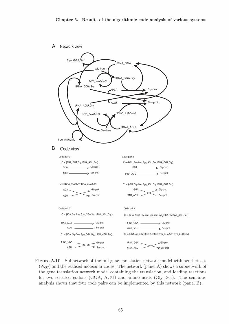
Chapter 5. Results of the algorithmic code analysis of various systems
Figure 5.10 Subnetwork of the full gene translation network model with synthetases(NGC) and the realised molecular codes. The network (panel A) shows a subnetwork ofthe gene translation network model containing the translation, and loading reactionsfor two selected codons (GGA, AGU) and amino acids (Gly, Ser). The semanticanalysis shows that four code pairs can be implemented by this network (panel B).
65
5.6. Gene regulatory networks
5.6 Gene regulatory networks
Biological background Cell’s maintain a complex regulatory system to orchestratethe expression of their genes. Different information about the external environmentand internal states are integrated to regulate the expression of proteins and enzymes.Regulation of gene expression is implemented differently in eukaryotes and prokaryotes,but share a common mechanism: proteins (transcription factors) need to bind the DNAto either activate or repress gene translation. In eukaryotes this process is much morecomplex, because also protein complexes are formed for this purpose. The gene regula-tory system of a cell is also a highly semantic system, because it carries and uses theinformation about the environment and internal (metabolic) states. This can be seenby analysing a gene regulatory network using the proposed algorithms.
A model of gene regulation To apply the code identifying algorithms at first anetwork model needs to be developed. In general, gene regulatory networks (GRN) aregraphs representing the regulation of the expression of certain genes by the expressionof other genes. A node in a GRN stands for a complex process including the gene,the promoter and binding region of that gene, the binding of the transcription factor(TF) plus cofactors and the production of a product by the recruitment of the geneexpression machinery. A cell’s GRN is also a highly semantic system based in molecularcodes. For the analysis a GRN is modelled as reaction network NGRN = 〈MGRN ,RGRN〉by explicitly inserting the relevant components (Fig 5.11). The resulting network isnot a generic model to describe all possible gene regulatory networks, but a model thatcovers the main properties of regulation important for this study. MGRN contains ntranscription factors TFi, m products Pj , and genes Gij . Each gene Gij represents acombination of a promoter site i and a coding region j, where the promoter site i isspecific to TFi and the coding region j produces Pj. For the model I assume that thereexist as many promoter sites and coding regions as transcription factors and products,respectively, such that each promoter-gene combination is possible. In summary
MGRN = {TF1, TF2, . . . , TFi, . . . , TFn, P1, P2, . . . ,
Pj , . . . , Pm, G11, G12, . . . , Gij, . . . , Gnm}.
The differences of eukaryotic and prokaryotic gene regulation, here, plays only a minorrole (and is not modelled) since only the general mechanism of transcription factorregulated expression shall be explored in a very basic approach.For the abstract model I will assume that a transcription factor binds only one promoterand that a promoter is bound by only one transcription factor. The assumption, thatone TF bind specifically only one promoter, and vice versa, is a broad simplification ofthe real biological system. Nevertheless, for the proof of principle presented here it isa reasonable one. The model could be made more complex (see below), but here it issufficient to describe the simpler model. The expression of a gene i, j then is given by
RGRN = {TFi +Gij → TFi +Gij + Pj} , i = 1, 2, . . . , n,
j = 1, 2, . . . , m.
Semantic analysis The semantic analysis shows that the reaction network can im-plement molecular codes, but only in one way, i.e. with the transcription factors as signs
66
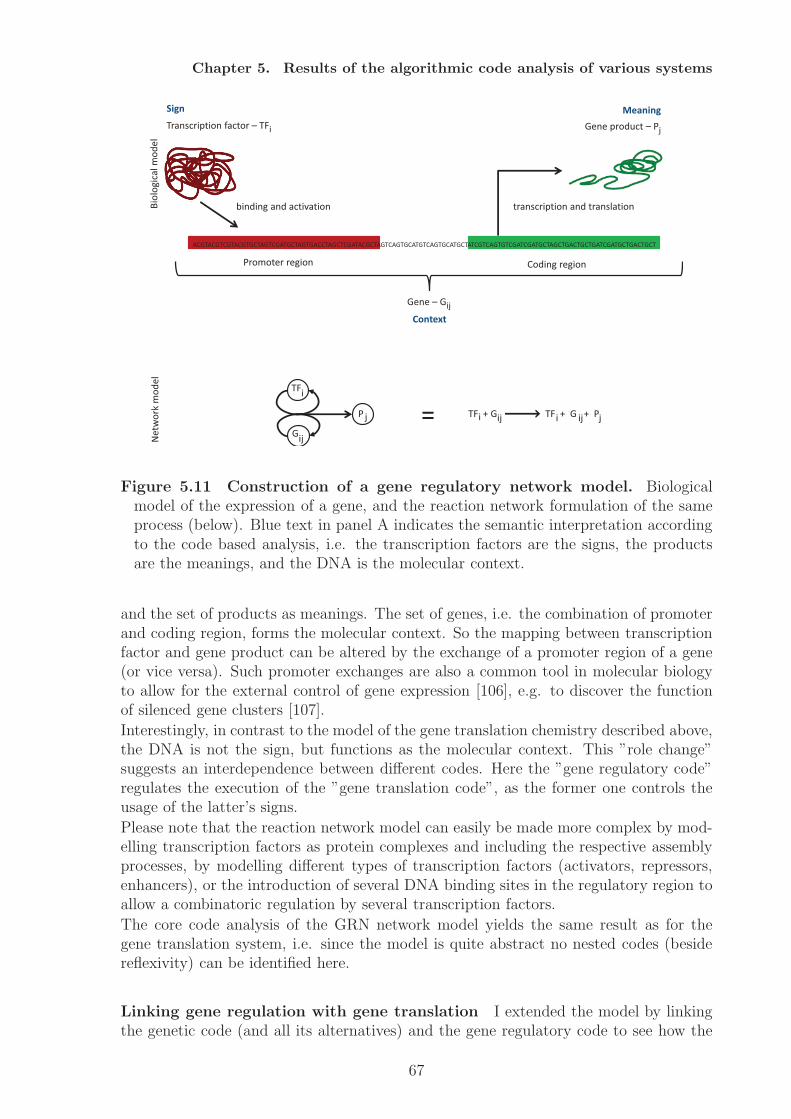
Chapter 5. Results of the algorithmic code analysis of various systems
Figure 5.11 Construction of a gene regulatory network model. Biologicalmodel of the expression of a gene, and the reaction network formulation of the sameprocess (below). Blue text in panel A indicates the semantic interpretation accordingto the code based analysis, i.e. the transcription factors are the signs, the productsare the meanings, and the DNA is the molecular context.
and the set of products as meanings. The set of genes, i.e. the combination of promoterand coding region, forms the molecular context. So the mapping between transcriptionfactor and gene product can be altered by the exchange of a promoter region of a gene(or vice versa). Such promoter exchanges are also a common tool in molecular biologyto allow for the external control of gene expression [106], e.g. to discover the functionof silenced gene clusters [107].
Interestingly, in contrast to the model of the gene translation chemistry described above,the DNA is not the sign, but functions as the molecular context. This ”role change”suggests an interdependence between different codes. Here the ”gene regulatory code”regulates the execution of the ”gene translation code”, as the former one controls theusage of the latter’s signs.
Please note that the reaction network model can easily be made more complex by mod-elling transcription factors as protein complexes and including the respective assemblyprocesses, by modelling different types of transcription factors (activators, repressors,enhancers), or the introduction of several DNA binding sites in the regulatory region toallow a combinatoric regulation by several transcription factors.
The core code analysis of the GRN network model yields the same result as for thegene translation system, i.e. since the model is quite abstract no nested codes (besidereflexivity) can be identified here.
Linking gene regulation with gene translation I extended the model by linkingthe genetic code (and all its alternatives) and the gene regulatory code to see how the
67
5.6. Gene regulatory networks
semantic capacity changes.A subnetwork of the model consists of two transcription factors TF1 and TF2, twobinding domains (promoters) P1 and P2, two coding regions of the genes, which aremodelled explicitly as strings ABA and BAB. The ”nucleic acids” A and B can betranslated to two amino acids L and K. As in the model above the two promotersare allowed to be freely combined with the two coding regions resulting in four genes.Resulting in four possible protein products defined by the tRNAs available, LLL, KKK,LKL, and KLK. The resulting reaction network contains 14 molecular species and 16reaction rules (see Appendix E 5 for the reaction network).This reaction network contains 13 binary molecular codes (Table 5.8). A closer lookto the resulting codes shows that molecular species from both subsystems (GRN, GC)can be used as signs, but only the final gene products can be meanings in these codes.While the molecular species from the GRN part can be combined as signs in one code(Table 5.8, codes 2-5), tRNAs are only combined with tRNAs as signs. In the molecularcontext all molecular species occur (except of the meanings).Codes 7 and 8 show that it is possible to implement a code based on one incoming signal(compare [80]). In both codes the signs contain the same promoter region, such thatthe alternative mappings can only be realised by a change in the genetic code, i.e. theselection of the specific tRNAs in the context.It is only possible to generate contingent mappings to the non-degenerated case, i.e.when A and B are encoded to different amino acids. The degenerated protein LLL,KKK are never used as meanings.The network combines several biochemical reactions and thus is only a rough model ofthe underlying processes. I extended the model by introducing the transcribed gene asintermediate product. By decoupling both processes the number of reactions reducesto 10, while the number of molecular species grows by the two transcripts ABA andBAB (for the network see Appendix E 5 ). This slightly different model now contains 27BMCs (Table 5.9). The difference in semantic capacity demonstrates that a code basedanalysis also is dependent on the level of detail of a given model. Structurally the codesfrom the simple and the extended model do not differ. The new codes are generated bythe meaning-sign-linkage (cp Section 3.4.3), because the transcripts now can be used assigns and meanings in the new codes.
68
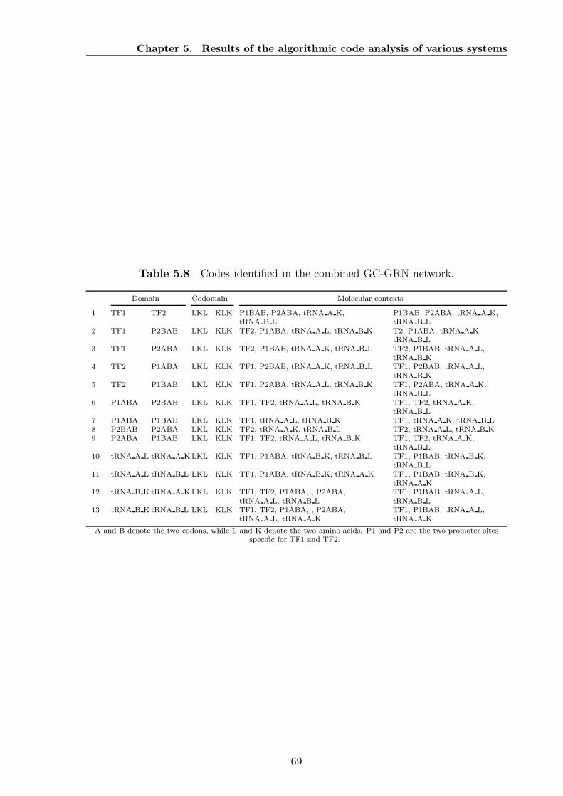
Chapter 5. Results of the algorithmic code analysis of various systems
Table 5.8 Codes identified in the combined GC-GRN network.
Domain Codomain Molecular contexts
1 TF1 TF2 LKL KLK P1BAB, P2ABA, tRNA A K,tRNA B L
P1BAB, P2ABA, tRNA A K,tRNA B L
2 TF1 P2BAB LKL KLK TF2, P1ABA, tRNA A L, tRNA B K T2, P1ABA, tRNA A K,tRNA B L
3 TF1 P2ABA LKL KLK TF2, P1BAB, tRNA A K, tRNA B L TF2, P1BAB, tRNA A L,tRNA B K
4 TF2 P1ABA LKL KLK TF1, P2BAB, tRNA A K, tRNA B L TF1, P2BAB, tRNA A L,tRNA B K
5 TF2 P1BAB LKL KLK TF1, P2ABA, tRNA A L, tRNA B K TF1, P2ABA, tRNA A K,tRNA B L
6 P1ABA P2BAB LKL KLK TF1, TF2, tRNA A L, tRNA B K TF1, TF2, tRNA A K,tRNA B L
7 P1ABA P1BAB LKL KLK TF1, tRNA A L, tRNA B K TF1, tRNA A K, tRNA B L8 P2BAB P2ABA LKL KLK TF2, tRNA A K, tRNA B L TF2, tRNA A L, tRNA B K9 P2ABA P1BAB LKL KLK TF1, TF2, tRNA A L, tRNA B K TF1, TF2, tRNA A K,
tRNA B L10 tRNA A L tRNA A KLKL KLK TF1, P1ABA, tRNA B K, tRNA B L TF1, P1BAB, tRNA B K,
tRNA B L11 tRNA A L tRNA B L LKL KLK TF1, P1ABA, tRNA B K, tRNA A K TF1, P1BAB, tRNA B K,
tRNA A K12 tRNA B K tRNA A KLKL KLK TF1, TF2, P1ABA, , P2ABA,
tRNA A L, tRNA B LTF1, P1BAB, tRNA A L,tRNA B L
13 tRNA B K tRNA B L LKL KLK TF1, TF2, P1ABA, , P2ABA,tRNA A L, tRNA A K
TF1, P1BAB, tRNA A L,tRNA A K
A and B denote the two codons, while L and K denote the two amino acids. P1 and P2 are the two promoter sitesspecific for TF1 and TF2.
69
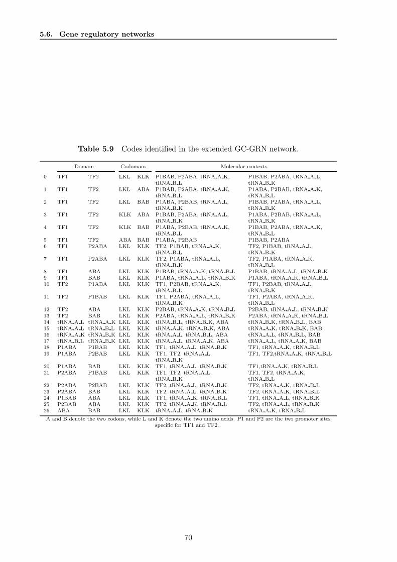
5.6. Gene regulatory networks
Table 5.9 Codes identified in the extended GC-GRN network.
Domain Codomain Molecular contexts
0 TF1 TF2 LKL KLK P1BAB, P2ABA, tRNA A K,tRNA B L
P1BAB, P2ABA, tRNA A L,tRNA B K
1 TF1 TF2 LKL ABA P1BAB, P2ABA, tRNA A K,tRNA B L
P1ABA, P2BAB, tRNA A K,tRNA B L
2 TF1 TF2 LKL BAB P1ABA, P2BAB, tRNA A L,tRNA B K
P1BAB, P2ABA, tRNA A L,tRNA B K
3 TF1 TF2 KLK ABA P1BAB, P2ABA, tRNA A L,tRNA B K
P1ABA, P2BAB, tRNA A L,tRNA B K
4 TF1 TF2 KLK BAB P1ABA, P2BAB, tRNA A K,tRNA B L
P1BAB, P2ABA, tRNA A K,tRNA B L
5 TF1 TF2 ABA BAB P1ABA, P2BAB P1BAB, P2ABA6 TF1 P2ABA LKL KLK TF2, P1BAB, tRNA A K,
tRNA B LTF2, P1BAB, tRNA A L,tRNA B K
7 TF1 P2ABA LKL KLK TF2, P1ABA, tRNA A L,tRNA B K
TF2, P1ABA, tRNA A K,tRNA B L
8 TF1 ABA LKL KLK P1BAB, tRNA A K, tRNA B L P1BAB, tRNA A L, tRNA B K9 TF1 BAB LKL KLK P1ABA, tRNA A L, tRNA B K P1ABA, tRNA A K, tRNA B L10 TF2 P1ABA LKL KLK TF1, P2BAB, tRNA A K,
tRNA B LTF1, P2BAB, tRNA A L,tRNA B K
11 TF2 P1BAB LKL KLK TF1, P2ABA, tRNA A L,tRNA B K
TF1, P2ABA, tRNA A K,tRNA B L
12 TF2 ABA LKL KLK P2BAB, tRNA A K, tRNA B L P2BAB, tRNA A L, tRNA B K13 TF2 BAB LKL KLK P2ABA, tRNA A L, tRNA B K P2ABA, tRNA A K, tRNA B L14 tRNA A L tRNA A K LKL KLK tRNA B L, tRNA B K, ABA tRNA B K, tRNA B L, BAB15 tRNA A L tRNA B L LKL KLK tRNA A K, tRNA B K, ABA tRNA A K, tRNA B K, BAB16 tRNA A K tRNA B K LKL KLK tRNA A L, tRNA B L, ABA tRNA A L, tRNA B L, BAB17 tRNA B L tRNA B K LKL KLK tRNA A L, tRNA A K, ABA tRNA A L, tRNA A K, BAB18 P1ABA P1BAB LKL KLK TF1, tRNA A L, tRNA B K TF1, tRNA A K, tRNA B L19 P1ABA P2BAB LKL KLK TF1, TF2, tRNA A L,
tRNA B KTF1, TF2,tRNA A K, tRNA B L
20 P1ABA BAB LKL KLK TF1, tRNA A L, tRNA B K TF1,tRNA A K, tRNA B L21 P2ABA P1BAB LKL KLK TF1, TF2, tRNA A L,
tRNA B KTF1, TF2, tRNA A K,tRNA B L
22 P2ABA P2BAB LKL KLK TF2, tRNA A L, tRNA B K TF2, tRNA A K, tRNA B L23 P2ABA BAB LKL KLK TF2, tRNA A L, tRNA B K TF2, tRNA A K, tRNA B L24 P1BAB ABA LKL KLK TF1, tRNA A K, tRNA B L TF1, tRNA A L, tRNA B K25 P2BAB ABA LKL KLK TF2, tRNA A K, tRNA B L TF2, tRNA A L, tRNA B K26 ABA BAB LKL KLK tRNA A L, tRNA B K tRNA A K, tRNA B L
A and B denote the two codons, while L and K denote the two amino acids. P1 and P2 are the two promoter sitesspecific for TF1 and TF2.
70
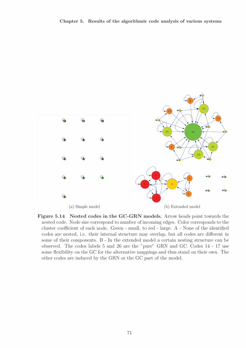
Chapter 5. Results of the algorithmic code analysis of various systems
9
12
3
6
0
2
10
4
11
78
5
1
(a) Simple model
2 3
8
6
1 0
2 0 2 6
1 8
2 5
9
1 91 2
7
2 2
1 3
2 4
1 7
1 4
2 1
1 5
1 1
1 64
2
1 5
3
0
(b) Extended model
Figure 5.14 Nested codes in the GC-GRN models. Arrow heads point towards thenested code. Node size correspond to number of incoming edges. Color corresponds to thecluster coefficient of each node. Green - small, to red - large. A - None of the identifiedcodes are nested, i.e. their internal structure may overlap, but all codes are different insome of their components. B - In the extended model a certain nesting structure can beobserved. The codes labels 5 and 26 are the ”pure” GRN and GC. Codes 14 - 17 usesome flexibility on the GC for the alternative mappings and thus stand on their own. Theother codes are induced by the GRN or the GC part of the model.
71
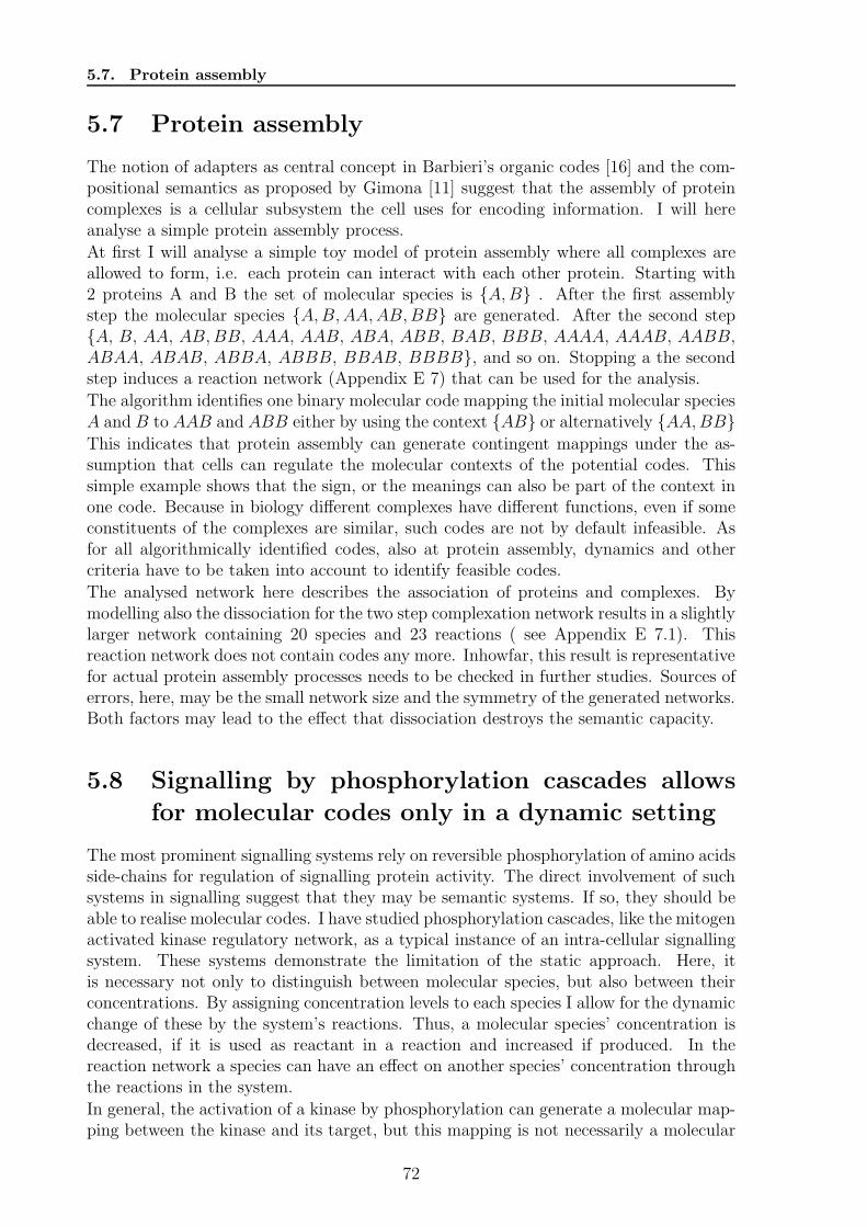
5.7. Protein assembly
5.7 Protein assembly
The notion of adapters as central concept in Barbieri’s organic codes [16] and the com-positional semantics as proposed by Gimona [11] suggest that the assembly of proteincomplexes is a cellular subsystem the cell uses for encoding information. I will hereanalyse a simple protein assembly process.
At first I will analyse a simple toy model of protein assembly where all complexes areallowed to form, i.e. each protein can interact with each other protein. Starting with2 proteins A and B the set of molecular species is {A,B} . After the first assemblystep the molecular species {A,B,AA,AB,BB} are generated. After the second step{A, B, AA, AB,BB, AAA, AAB, ABA, ABB, BAB, BBB, AAAA, AAAB, AABB,ABAA, ABAB, ABBA, ABBB, BBAB, BBBB}, and so on. Stopping a the secondstep induces a reaction network (Appendix E 7) that can be used for the analysis.
The algorithm identifies one binary molecular code mapping the initial molecular speciesA and B to AAB and ABB either by using the context {AB} or alternatively {AA,BB}This indicates that protein assembly can generate contingent mappings under the as-sumption that cells can regulate the molecular contexts of the potential codes. Thissimple example shows that the sign, or the meanings can also be part of the context inone code. Because in biology different complexes have different functions, even if someconstituents of the complexes are similar, such codes are not by default infeasible. Asfor all algorithmically identified codes, also at protein assembly, dynamics and othercriteria have to be taken into account to identify feasible codes.
The analysed network here describes the association of proteins and complexes. Bymodelling also the dissociation for the two step complexation network results in a slightlylarger network containing 20 species and 23 reactions ( see Appendix E 7.1). Thisreaction network does not contain codes any more. Inhowfar, this result is representativefor actual protein assembly processes needs to be checked in further studies. Sources oferrors, here, may be the small network size and the symmetry of the generated networks.Both factors may lead to the effect that dissociation destroys the semantic capacity.
5.8 Signalling by phosphorylation cascades allows
for molecular codes only in a dynamic setting
The most prominent signalling systems rely on reversible phosphorylation of amino acidsside-chains for regulation of signalling protein activity. The direct involvement of suchsystems in signalling suggest that they may be semantic systems. If so, they should beable to realise molecular codes. I have studied phosphorylation cascades, like the mitogenactivated kinase regulatory network, as a typical instance of an intra-cellular signallingsystem. These systems demonstrate the limitation of the static approach. Here, itis necessary not only to distinguish between molecular species, but also between theirconcentrations. By assigning concentration levels to each species I allow for the dynamicchange of these by the system’s reactions. Thus, a molecular species’ concentration isdecreased, if it is used as reactant in a reaction and increased if produced. In thereaction network a species can have an effect on another species’ concentration throughthe reactions in the system.
In general, the activation of a kinase by phosphorylation can generate a molecular map-ping between the kinase and its target, but this mapping is not necessarily a molecular
72
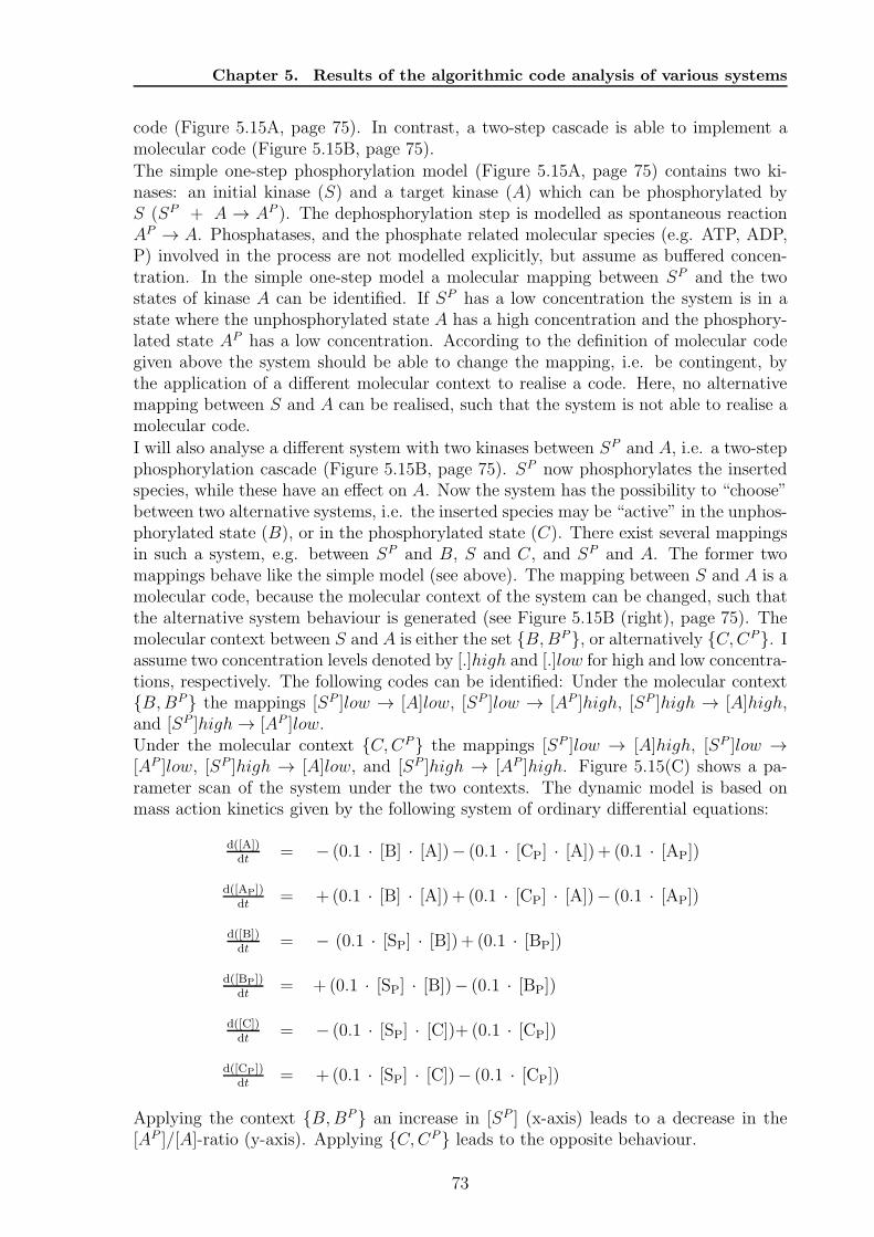
Chapter 5. Results of the algorithmic code analysis of various systems
code (Figure 5.15A, page 75). In contrast, a two-step cascade is able to implement amolecular code (Figure 5.15B, page 75).
The simple one-step phosphorylation model (Figure 5.15A, page 75) contains two ki-nases: an initial kinase (S) and a target kinase (A) which can be phosphorylated byS (SP + A → AP ). The dephosphorylation step is modelled as spontaneous reactionAP → A. Phosphatases, and the phosphate related molecular species (e.g. ATP, ADP,P) involved in the process are not modelled explicitly, but assume as buffered concen-tration. In the simple one-step model a molecular mapping between SP and the twostates of kinase A can be identified. If SP has a low concentration the system is in astate where the unphosphorylated state A has a high concentration and the phosphory-lated state AP has a low concentration. According to the definition of molecular codegiven above the system should be able to change the mapping, i.e. be contingent, bythe application of a different molecular context to realise a code. Here, no alternativemapping between S and A can be realised, such that the system is not able to realise amolecular code.
I will also analyse a different system with two kinases between SP and A, i.e. a two-stepphosphorylation cascade (Figure 5.15B, page 75). SP now phosphorylates the insertedspecies, while these have an effect on A. Now the system has the possibility to “choose”between two alternative systems, i.e. the inserted species may be “active” in the unphos-phorylated state (B), or in the phosphorylated state (C). There exist several mappingsin such a system, e.g. between SP and B, S and C, and SP and A. The former twomappings behave like the simple model (see above). The mapping between S and A is amolecular code, because the molecular context of the system can be changed, such thatthe alternative system behaviour is generated (see Figure 5.15B (right), page 75). Themolecular context between S and A is either the set {B,BP}, or alternatively {C,CP}. Iassume two concentration levels denoted by [.]high and [.]low for high and low concentra-tions, respectively. The following codes can be identified: Under the molecular context{B,BP} the mappings [SP ]low → [A]low, [SP ]low → [AP ]high, [SP ]high → [A]high,and [SP ]high→ [AP ]low.Under the molecular context {C,CP} the mappings [SP ]low → [A]high, [SP ]low →[AP ]low, [SP ]high → [A]low, and [SP ]high → [AP ]high. Figure 5.15(C) shows a pa-rameter scan of the system under the two contexts. The dynamic model is based onmass action kinetics given by the following system of ordinary differential equations:
d([A])dt
= − (0.1 · [B] · [A])− (0.1 · [CP] · [A]) + (0.1 · [AP])
d([AP])dt
= + (0.1 · [B] · [A]) + (0.1 · [CP] · [A])− (0.1 · [AP])
d([B])dt
= − (0.1 · [SP] · [B])+ (0.1 · [BP])
d([BP])dt
= + (0.1 · [SP] · [B])− (0.1 · [BP])
d([C])dt
= − (0.1 · [SP] · [C])+ (0.1 · [CP])
d([CP])dt
= + (0.1 · [SP] · [C])− (0.1 · [CP])
Applying the context {B,BP} an increase in [SP ] (x-axis) leads to a decrease in the[AP ]/[A]-ratio (y-axis). Applying {C,CP} leads to the opposite behaviour.
73

5.8. Signalling by phosphorylation cascades.
The extension of the static approach to a dynamic setting needs more strict definitions,such that the here shown properties are only a first step into this direction. For thediscussion of potential extensions see Chapter 6 ”Towards pragmatics”(pp. 85).
74
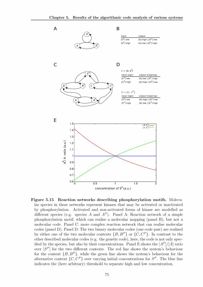
Chapter 5. Results of the algorithmic code analysis of various systems
Figure 5.15 Reaction networks describing phosphorylation motifs. Molecu-lar species in these networks represent kinases that may be activated or inactivatedby phosphorylation. Activated and non-activated forms of kinase are modelled asdifferent species (e.g. species A and AP ). Panel A: Reaction network of a simplephosphorylation motif, which can realise a molecular mapping (panel B), but not amolecular code. Panel C: more complex reaction network that can realise molecularcodes (panel D). Panel D: The two binary molecular codes (one code pair) are realisedby either one of the two molecular contexts {B,BP} or {C,CP}. In contrast to theother described molecular codes (e.g. the genetic code), here, the code is not only spec-ified by the species, but also by their concentrations. Panel E shows the [AP ]/[A] ratioover [SP ] for the two different contexts. The red line shows the system’s behaviourfor the context {B,BP}, while the green line shows the system’s behaviour for thealternative context {C,CP} over varying initial concentrations for SP . The blue lineindicates the (here arbitrary) threshold to separate high and low concentration.
75
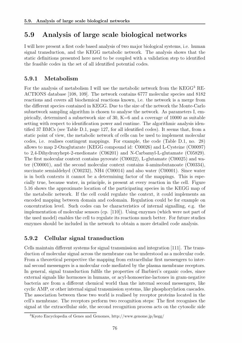
5.9. Analysis of large scale biological networks
5.9 Analysis of large scale biological networks
I will here present a first code based analysis of two major biological systems, i.e. humansignal transduction, and the KEGG metabolic network. The analysis shows that thestatic definitions presented here need to be coupled with a validation step to identifiedthe feasible codes in the set of all identified potential codes.
5.9.1 Metabolism
For the analysis of metabolism I will use the metabolic network from the KEGG3 RE-ACTIONS database [108, 109]. The network contains 6777 molecular species and 8182reactions and covers all biochemical reactions known, i.e. the network is a merge fromthe different species contained in KEGG. Due to the size of the network the Monte-Carlosubnetwork sampling algorithm is chosen to analyse the network. As parameters I, em-pirically, determined a subnetwork size of 30, K=6 and a coverage of 10000 as suitablesetting with respect to identification power and runtime. The algorithmic analysis iden-tified 37 BMCs (see Table D.1, page 127, for all identified codes). It seems that, from astatic point of view, the metabolic network of cells can be used to implement molecularcodes, i.e. realises contingent mappings. For example, the code (Table D.1, no. 28)allows to map 2-Oxoglutarate (KEGG compound id: C00026) and L-Cysteine (C00097)to 2,4-Dihydroxyhept-2-enedionate (C06201) and N-Carbamyl-L-glutamate (C05829).The first molecular context contains pyrovate (C00022), L-glutamate (C00025) and wa-ter (C00001), and the second molecular context contains 4-aminobutanoate (C00334),succinate semialdehyd (C00232), NH4 (C00014) and also water (C00001). Since wateris in both contexts it cannot be a determining factor of the mappings. This is espe-cially true, because water, in principle, is present at every reaction in the cell. Figure5.16 shows the approximate location of the participating species in the KEGG map ofthe metabolic network. If the cell could regulate the context, it could implements anencoded mapping between domain and codomain. Regulation could be for example onconcentration level. Such codes can be characteristics of internal signalling, e.g. theimplementation of molecular sensors (cp. [110]). Using enzymes (which were not part ofthe used model) enables the cell to regulate its reactions much better. For future studiesenzymes should be included in the network to obtain a more detailed code analysis.
5.9.2 Cellular signal transduction
Cells maintain different systems for signal transmission and integration [111]. The trans-duction of molecular signal across the membrane can be understood as a molecular code.From a theoretical perspective the mapping from extracellular first messengers to inter-nal second messengers is a molecular code mediated by the plasma membrane receptors.In general, signal transduction fulfils the properties of Barbieri’s organic codes, sinceexternal signals like hormones in humans, or acyl-homoserine-lactones in gram-negativebacteria are from a different chemical world than the internal second messengers, likecyclic AMP, or other internal signal transmission systems, like phosphorylation cascades.The association between these two world is realised by receptor proteins located in thecell’s membrane. The receptors perform two recognition steps: The first recognises thesignal at the extracellular side, the second recognition process acts on the cytosolic side
3Kyoto Encyclopedia of Genes and Genomes, http://www.genome.jp/kegg/
76
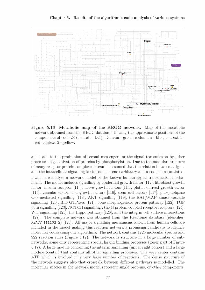
Chapter 5. Results of the algorithmic code analysis of various systems
Figure 5.16 Metabolic map of the KEGG network. Map of the metabolicnetwork obtained from the KEGG database showing the approximate positions of thecomponents of code 28 (cf. Table D.1). Domain - green, codomain - blue, context 1 -red, context 2 - yellow.
and leads to the production of second messengers or the signal transmission by otherprocesses, e.g. activation of proteins by phosphorylation. Due to the modular structureof many receptor protein complexes it can be assumed that the relation between a signaland the intracellular signalling is (to some extend) arbitrary and a code is instantiated.
I will here analyse a network model of the known human signal transduction mecha-nisms. The model includes signalling by epidermal growth factor [112], fibroblast growthfactor, insulin receptor [113], nerve growth factors [114], platlet-derived growth factor[115], vascular endothelial growth factors [116], stem cell factors [117], phospholipaseC-γ mediated signalling [118], AKT signalling [119], the RAF/MAP kinase cascadesignalling [120], Rho GTPases [121], bone morphogenetic protein pathway [122], TGFbeta signalling [123], NOTCH signalling , the G protein coupled receptor receptors [124],Wnt signalling [125], the Hippo pathway [126], and the integrin cell surface interactions[127]. The complete network was obtained from the Reactome database (identifier:REACT 111102.2) [128]. All major signalling mechanisms known from human cells areincluded in the model making this reaction network a promising candidate to identifymolecular codes using our algorithms. The network contains 1725 molecular species and922 reaction rules (Figure 5.17). The network is structure in a large number of sub-networks, some only representing special ligand binding processes (lower part of Figure5.17). A large module containing the integrin signalling (upper right corner) and a largemodule (center) that contains all other signalling processes. The very center containsATP which is involved in a very large number of reactions. The dense structure ofthe network suggests also that crosstalk between different pathways is modelled. Themolecular species in the network model represent single proteins, or other components,
77
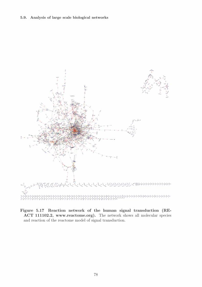
5.9. Analysis of large scale biological networks
Figure 5.17 Reaction network of the human signal transduction (RE-ACT 111102.2, www.reactome.org). The network shows all molecular speciesand reaction of the reactome model of signal transduction.
78
Chapter 5. Results of the algorithmic code analysis of various systems
but also can stand for general families of molecular species, e.g. the species ”GPCRthat activates Gi[plasmamembrane]”. Species’ intracellular localisation is given by thetags ”[plasmamembran]”,”[cytosol]”, and ”[extracellular]”, or combinations thereof inthe case of some complexes.
To analyse this network I use, due to the large size, the Monte-Carlo subnetwork sam-pling heuristic. For this network a reasonable subnetwork size (50), a small value of K(1) and a coverage rate of 100000 empirically proved suitable. The algorithm results in558 binary molecular codes.
I defined seven biological roles to access the codes structures: cofactors (COF) forall proteins of other molecules necessary for the signalling, but which are not activelyparticipating, effectors (EFF) like adenylate cyclase that produces second messengers,ligands (L), receptors (R), ligand receptor complexes (LR), activated receptors (AR),molecules and proteins that just transmit the signal (ST) and second messengers (SM).Table C.1 in Appendix C summarises which molecular species have been identified inwhich semiotics role (sign, meaning, context) among the codes and also gives informationabout the assigned role.
Analysis of the participating molecular species First I analysed if the identifiedmolecular species occur either exclusively as signs (meanings) or if multiple roles can betaken by a species. Therefore, I determined the indicator variables Is(a), Im(a) ∈ {0, 1},i.e. a molecular species a participated in at least one code either as sign or as meaning,respectively. Table 5.10 shows the contingency table of the two variables. A χ2 test onthe data show no significant dependency between the two groups ”used as sign” and”used as meaning” (χ2 = 2.12, p = 0.146).
Table 5.10 Contingency table of biological roles of participating molecular species.
Is\Im 0 10 146 421 31 15
For the analysis of the identified molecular species that could participate in a code Icounted the number of codes for each species where it can act either as sign, meaningor context. Many of the identified molecular species (146 of 234) are neither used assign or meaning, but only as context. One third of the species (73) is used exclusivelyeither as sign or meaning and only 15 species are used as both. The molecular speciesthat can function as sign and meaning in different codes are classified mainly as signaltransducing species (10), but also as ligand receptor complexes (6) and cofactors andeffectors (1 each). All molecular species are complexes involving GTP or GDP, andGDP itself, which can also be used as sign and meaning.
Table 5.11 shows the results of the analysis of the biological role versus the semiotic role.The analysis of the medians shows that over all biological roles many of the molecularspecies are never used as signs or meanings (medians are zero) but more often as context.This is due to the higher proportion of molecular species that can act only in contexts.The analysis of the means is qualitatively the same (context > sign, meaning), butdiffers in the actual values. A further statistical analysis, e.g. to identify differencesbetween the biological roles, seems not very promising on this dataset, because t-testson the means can not be applied due to non-normality of the (empirical) distributions
79
5.9. Analysis of large scale biological networks
and also non-parametric rank-test (e.g. a U-Test) are not very powerful here, becausethe medians are very similar (many zeros).
Table 5.11 Number of codes per semiotic role for the biological roles.
median number of codes mean number of codes
biological role N signs meanings context signs meanings context
AR 20 0 0 2.5 7.8 2.15 5.65LR 57 0 0 4 4.89 7.46 15.30R 23 0 0 1 1.47 2.43 3.39L 5 0 1 0 3.6 5 3.6ST 96 0 1 4 7.5 7.76 40.56SM 1 0 0 5 0 0 5COF 20 0 0 7 12.5 2.15 29.25EFF 12 0 0.5 8.5 4.25 1.91 33.67
Analysing the code structures Structurally, the identified codes are not as ex-pected, mainly between external ligands and internal second messengers (classical code),but can be found in any combination of biological roles, also with receptors as mean-ings for example. The most abundant combination are codes where a ligand boundreceptor and a signal transduction molecule can be mapped to two signal transduc-tion molecules. The second most abundant combination is similar, but maps a signaltransduction molecule and a ligand bound receptor to a signal transduction moleculeand a ligand bound receptor. This is a combination where a receptor is a meaning. Ifthese codes could be really used by cells, e.g. for any kind of internal controls can beonly determined by a dynamic validation. Table 5.12 summarises the combinations ofbiological roles that have been found together in a code sorted by abundance.A proper validation, e.g. by expert knowledge and dynamical arguments, is necessaryto identify the feasible codes which might lead to a reduced set of molecular codes.A different set of parameter values for the algorithmic code identification certainly wouldresult in a larger number of BMCs.
80
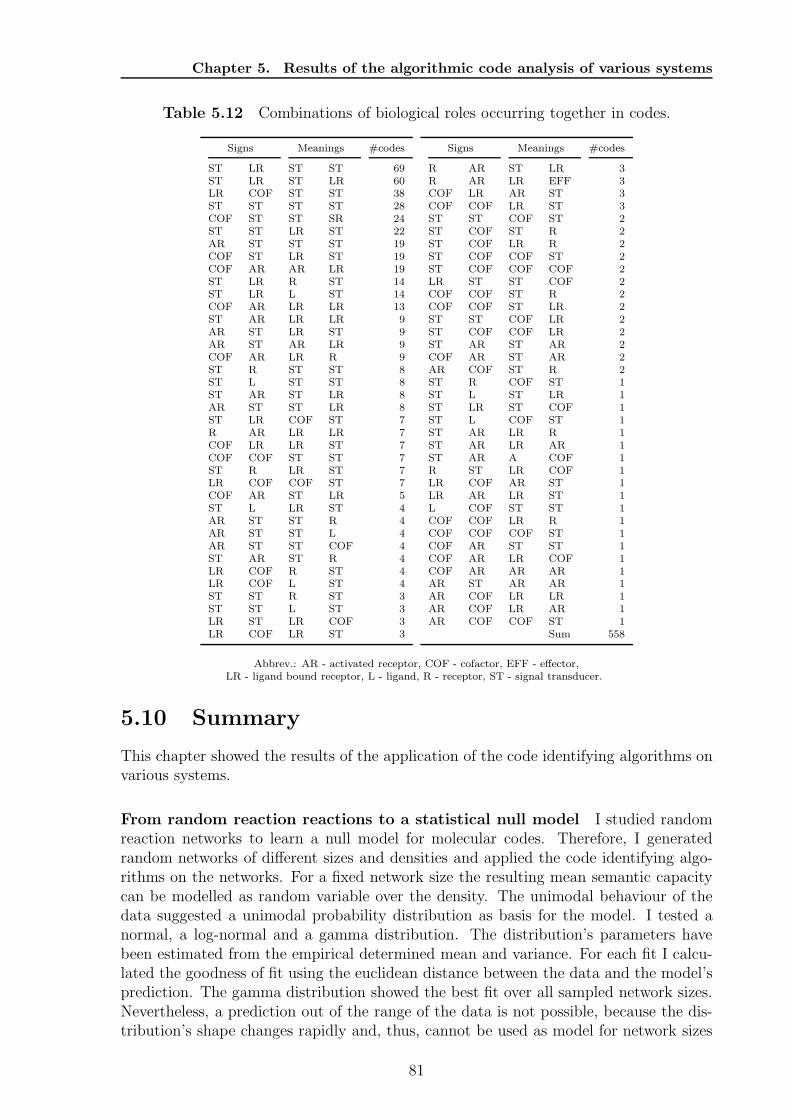
Chapter 5. Results of the algorithmic code analysis of various systems
Table 5.12 Combinations of biological roles occurring together in codes.
Signs Meanings #codes
ST LR ST ST 69ST LR ST LR 60LR COF ST ST 38ST ST ST ST 28COF ST ST SR 24ST ST LR ST 22AR ST ST ST 19COF ST LR ST 19COF AR AR LR 19ST LR R ST 14ST LR L ST 14COF AR LR LR 13ST AR LR LR 9AR ST LR ST 9AR ST AR LR 9COF AR LR R 9ST R ST ST 8ST L ST ST 8ST AR ST LR 8AR ST ST LR 8ST LR COF ST 7R AR LR LR 7COF LR LR ST 7COF COF ST ST 7ST R LR ST 7LR COF COF ST 7COF AR ST LR 5ST L LR ST 4AR ST ST R 4AR ST ST L 4AR ST ST COF 4ST AR ST R 4LR COF R ST 4LR COF L ST 4ST ST R ST 3ST ST L ST 3LR ST LR COF 3LR COF LR ST 3
Signs Meanings #codes
R AR ST LR 3R AR LR EFF 3COF LR AR ST 3COF COF LR ST 3ST ST COF ST 2ST COF ST R 2ST COF LR R 2ST COF COF ST 2ST COF COF COF 2LR ST ST COF 2COF COF ST R 2COF COF ST LR 2ST ST COF LR 2ST COF COF LR 2ST AR ST AR 2COF AR ST AR 2AR COF ST R 2ST R COF ST 1ST L ST LR 1ST LR ST COF 1ST L COF ST 1ST AR LR R 1ST AR LR AR 1ST AR A COF 1R ST LR COF 1LR COF AR ST 1LR AR LR ST 1L COF ST ST 1COF COF LR R 1COF COF COF ST 1COF AR ST ST 1COF AR LR COF 1COF AR AR AR 1AR ST AR AR 1AR COF LR LR 1AR COF LR AR 1AR COF COF ST 1
Sum 558
Abbrev.: AR - activated receptor, COF - cofactor, EFF - effector,LR - ligand bound receptor, L - ligand, R - receptor, ST - signal transducer.
5.10 Summary
This chapter showed the results of the application of the code identifying algorithms onvarious systems.
From random reaction reactions to a statistical null model I studied randomreaction networks to learn a null model for molecular codes. Therefore, I generatedrandom networks of different sizes and densities and applied the code identifying algo-rithms on the networks. For a fixed network size the resulting mean semantic capacitycan be modelled as random variable over the density. The unimodal behaviour of thedata suggested a unimodal probability distribution as basis for the model. I tested anormal, a log-normal and a gamma distribution. The distribution’s parameters havebeen estimated from the empirical determined mean and variance. For each fit I calcu-lated the goodness of fit using the euclidean distance between the data and the model’sprediction. The gamma distribution showed the best fit over all sampled network sizes.Nevertheless, a prediction out of the range of the data is not possible, because the dis-tribution’s shape changes rapidly and, thus, cannot be used as model for network sizes
81
5.10. Summary
larger than 25. For a prediction of the semantic capacity for network sizes in the rangeof the data the model is well suited. The very basic approach to generate random net-works can be extended by, for example, generating random network maintaining somenetwork properties, e.g., node degrees (in/out), or reconstitute the order distribution ofthe contained reactions. Also the identified codes have not been filtered, for example,for core codes, thus the exponential growth of the code pairs may be a result of sucheffects.
The general fact that codes can be found also in random networks can also be interpretedwith respect to the evolution of codes. It shows, that by random variation of the reactionnetwork potential codes can be introduced into a system. To really use a code the systemneed to be able to regulate the code’s context, either dynamically or on an evolutionarytime scale (cf. Chapter 6).
Combustion chemistries and biological networks The analysis of a set of com-bustion chemistries supported the hypothesis that the implementation of arbitrary map-pings may be an exclusive feature of biological systems. None of the analysed combustionchemistries contained codes. This result is strengthened by the fact that these networksare considered to be complete in the sense that all reactions that could happen amongthe contained molecular species are contained in the network model.
The analysed biological networks all (beside the merge of the genetic codes) have beenobtained by a knowledge based approach, i.e. the reactions have been modelled based onexpert knowledge about the system. This approach has been chosen, because networkmodels from database are not complete, firstly, because scientific progress in the respec-tive field does not yet yield complete model, and secondly, because biological systemsonly realise one of the potential mappings. In the latter case also more effort in researchmight not result in the detection of the specific reactions necessary for the code basedanalysis. The analysis of the merge network of known genetic codes shows that mergingnetworks may be a suitable approach to acquire suitable network models. Such mergingneeds to be done carefully. It may only make sense if network models from the sameenvironmental context are merged, like the genetic codes.
The detailed analysis of the gene translation systems of cells showed that depending onthe level of detail of the model the results of a code based analysis can be different. Here,the additional modelling of the amino acyl synthetases increased the semantic capacityof the system.
The coupling with the gene regulatory network, which is also a highly semantic systemon its own, showed how a meaning-sign-linkage effects the semantic capacity.
I analysed simple protein assembly networks and showed that in general codes canbe formed with such systems, but dissociation can destroy this property. A detailedanalysis of an actual biological protein assembly network, as for example in kinetochoreassembly may be a promising target for further research so see whether the influence ofdissociation is also important in real systems.
Large scale biological systems The analysis of large scale biological systems showedthat also in network models derived from experiments codes can be found. I demon-strated that without a subsequent validation of the codes no proper estimation of thesemantic capacity can be given. The huge amount of potential codes, either due to astrong fan-in/fan-out (cf. code nesting, Section 3.4) or the large network sizes lead to
82
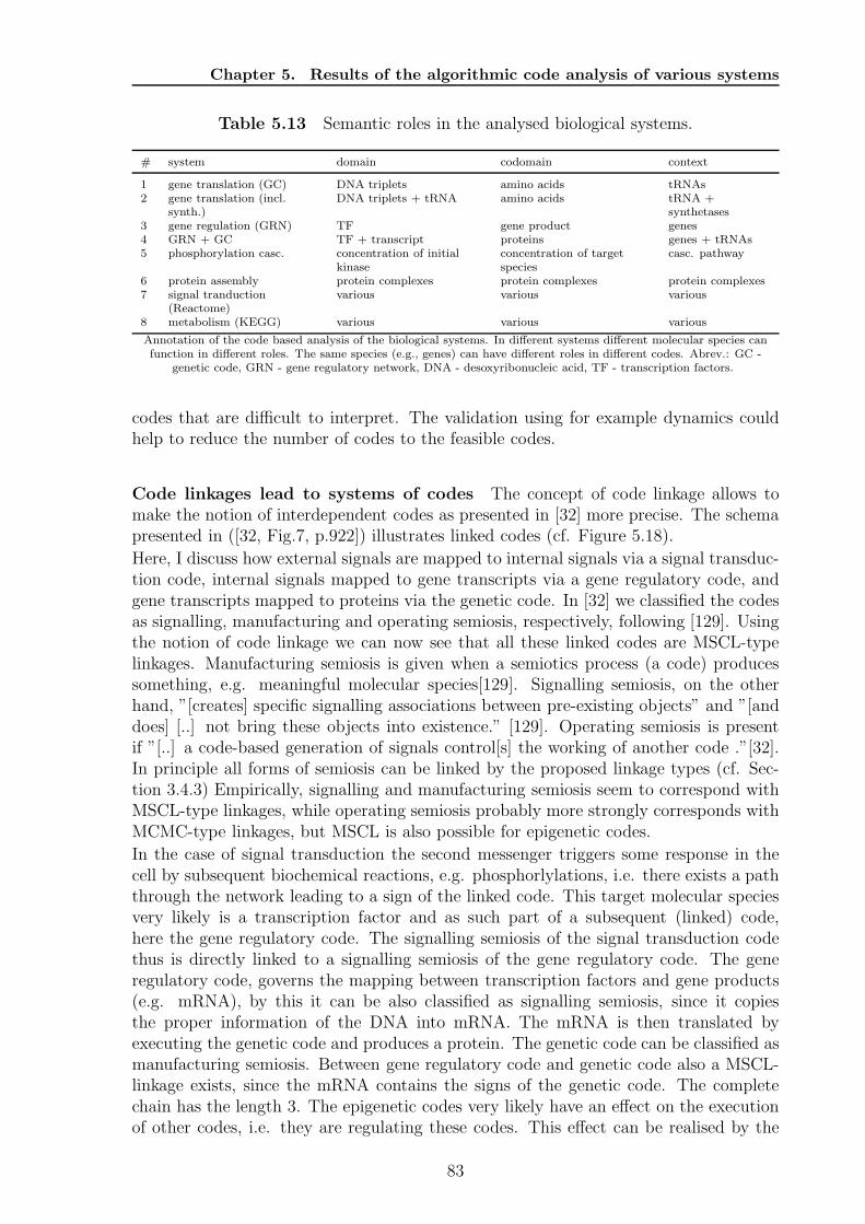
Chapter 5. Results of the algorithmic code analysis of various systems
Table 5.13 Semantic roles in the analysed biological systems.
# system domain codomain context
1 gene translation (GC) DNA triplets amino acids tRNAs2 gene translation (incl.
synth.)DNA triplets + tRNA amino acids tRNA +
synthetases3 gene regulation (GRN) TF gene product genes4 GRN + GC TF + transcript proteins genes + tRNAs5 phosphorylation casc. concentration of initial
kinaseconcentration of targetspecies
casc. pathway
6 protein assembly protein complexes protein complexes protein complexes7 signal tranduction
(Reactome)various various various
8 metabolism (KEGG) various various various
Annotation of the code based analysis of the biological systems. In different systems different molecular species canfunction in different roles. The same species (e.g., genes) can have different roles in different codes. Abrev.: GC -
genetic code, GRN - gene regulatory network, DNA - desoxyribonucleic acid, TF - transcription factors.
codes that are difficult to interpret. The validation using for example dynamics couldhelp to reduce the number of codes to the feasible codes.
Code linkages lead to systems of codes The concept of code linkage allows tomake the notion of interdependent codes as presented in [32] more precise. The schemapresented in ([32, Fig.7, p.922]) illustrates linked codes (cf. Figure 5.18).
Here, I discuss how external signals are mapped to internal signals via a signal transduc-tion code, internal signals mapped to gene transcripts via a gene regulatory code, andgene transcripts mapped to proteins via the genetic code. In [32] we classified the codesas signalling, manufacturing and operating semiosis, respectively, following [129]. Usingthe notion of code linkage we can now see that all these linked codes are MSCL-typelinkages. Manufacturing semiosis is given when a semiotics process (a code) producessomething, e.g. meaningful molecular species[129]. Signalling semiosis, on the otherhand, ”[creates] specific signalling associations between pre-existing objects” and ”[anddoes] [..] not bring these objects into existence.” [129]. Operating semiosis is presentif ”[..] a code-based generation of signals control[s] the working of another code .”[32].In principle all forms of semiosis can be linked by the proposed linkage types (cf. Sec-tion 3.4.3) Empirically, signalling and manufacturing semiosis seem to correspond withMSCL-type linkages, while operating semiosis probably more strongly corresponds withMCMC-type linkages, but MSCL is also possible for epigenetic codes.
In the case of signal transduction the second messenger triggers some response in thecell by subsequent biochemical reactions, e.g. phosphorlylations, i.e. there exists a paththrough the network leading to a sign of the linked code. This target molecular speciesvery likely is a transcription factor and as such part of a subsequent (linked) code,here the gene regulatory code. The signalling semiosis of the signal transduction codethus is directly linked to a signalling semiosis of the gene regulatory code. The generegulatory code, governs the mapping between transcription factors and gene products(e.g. mRNA), by this it can be also classified as signalling semiosis, since it copiesthe proper information of the DNA into mRNA. The mRNA is then translated byexecuting the genetic code and produces a protein. The genetic code can be classified asmanufacturing semiosis. Between gene regulatory code and genetic code also a MSCL-linkage exists, since the mRNA contains the signs of the genetic code. The completechain has the length 3. The epigenetic codes very likely have an effect on the executionof other codes, i.e. they are regulating these codes. This effect can be realised by the
83
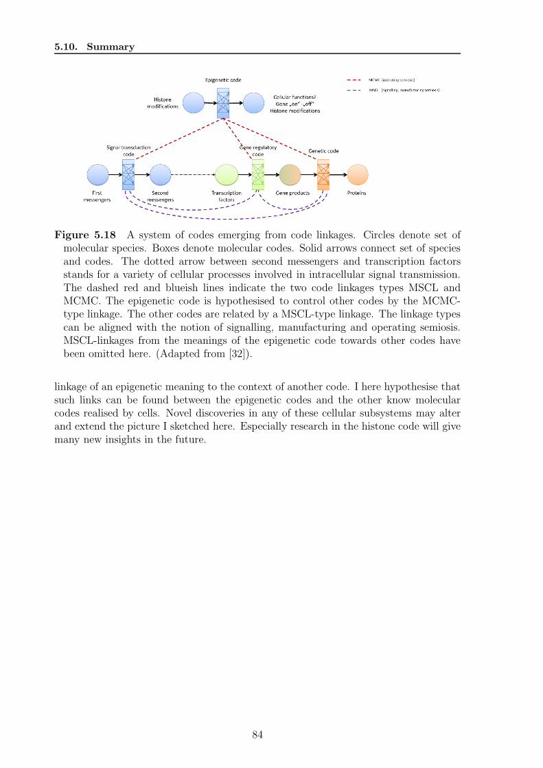
5.10. Summary
Figure 5.18 A system of codes emerging from code linkages. Circles denote set ofmolecular species. Boxes denote molecular codes. Solid arrows connect set of speciesand codes. The dotted arrow between second messengers and transcription factorsstands for a variety of cellular processes involved in intracellular signal transmission.The dashed red and blueish lines indicate the two code linkages types MSCL andMCMC. The epigenetic code is hypothesised to control other codes by the MCMC-type linkage. The other codes are related by a MSCL-type linkage. The linkage typescan be aligned with the notion of signalling, manufacturing and operating semiosis.MSCL-linkages from the meanings of the epigenetic code towards other codes havebeen omitted here. (Adapted from [32]).
linkage of an epigenetic meaning to the context of another code. I here hypothesise thatsuch links can be found between the epigenetic codes and the other know molecularcodes realised by cells. Novel discoveries in any of these cellular subsystems may alterand extend the picture I sketched here. Especially research in the histone code will givemany new insights in the future.
84
Chapter 6
Towards pragmatics
In this chapter I want to present a number of ideas that lead from the pure semantic,structural level to the dynamic, pragmatic level of molecular codes.
6.1 Code validation
Dynamic code validation The analysis of photochemistries (Section 5.4), metabolism(Section 5.9.1) and signal transduction (Section 5.9.2) demonstrated that algorithmicallyidentified molecular codes may need some kind of subsequent validation. This validationis necessary, because the definition, and thus the algorithms, neglects the dynamics ofthe system. In the case of the photochemistries light could have been used for an en-coded mapping (structural information), but because this was in the night-side model nolight should be present (dynamic information). For metabolism and signal transductionfor many of the found codes dynamics may lead to non-injective mappings, i.e. whenboth contexts are realised simultaneously. Generalising this idea leads to the notion ofcode validation.Given a molecular code f and all its alternative mappings gi we say f is valid if at anytime interval in the system’s time course
1. all elements of one molecular context of f are present either simultaneously, orsequentially.
2. no two alternative contexts are present at the same time.
The definition basically requires that in the dynamic execution of the system the molec-ular context should be present in such a manner that the mapping can be executedand that non of the other mappings can be executed simultaneously, to obtain a uniquemapping. Algorithmically, this can be checked by computer simulations. We can alsouse this information to adjust the semantic capacity to the number of valid codes.The validation step could also be performed in wet-lab experiments. The definition ofsuch experiments could orientate basically at the formulation of the code-identifyingalgorithms, i.e. mixing one sign and the molecular context should result in the presenceof one respective meaning. The advantage of an experimental validation, especially in-vivo, is that the system is complete, and thus wrongly identified codes, e.g. because ofincomplete network models, can be ruled out.
Code probability Beside the dynamic and experimental validation, more generally,we can try to calculate a code’s probability.
85
6.1. Code validation
Relevant questions in this regard are:
1. Given a molecular code which of the alternative mappings has the maximal prob-ability. under realistic assumptions?
2. Given a set of molecular codes of a network, which code has the maximal proba-bility, under realistic assumptions?
Both questions are similar, but tackle different aspects of a system’s semantic capacity.Question (1) asks for the probability of one (unique) realisation of a code, i.e. whichalternative context is chosen (cf. code determination in the next section)? Question (2)focusses on the overall semantic capacity.Answering these questions only makes sense under realistic conditions. By this I meanthat all relevant parameters, like kinetic rates, temperature, pH, concentrations, justto mention a few, have to be modelled in realistic ranges. In general, each mapping’s
f : AC7→ B probability P (f) can be defined via the implied reactions ρ ∈ R leading to
P (f) =∏
ρ
P (ρ).
Assuming a well-stirred reaction vessel the probability of reaction ρ to fire is given by
P (ρ) = P (reactants collide) · P (reactants react on collision).
The probability for a collision is given by the reactants concentrations, while the prob-ability that the reaction happens can be any constant or dependent on the actual reac-tants.A s-t path’s pts probability is given by
P (pts) =∏
ρ∈pts
P (ρ).
For a dynamic framework time can also be included in the probabilities, i.e. reactantsneed not only to be in vicinity to each other, but also be present at the same time.For a BMC between {A1, A2} and {B1, B2} there exists the four paths pB1
A1, pB2
A1, pB1
A2,
pB2A2. A unique mapping is given in the determining cases that the probabilities P (pB1
A1)+
P (pB2A2) = 0 (implying that P (pB2
A1) + P (pB1
A2) 6= 0) or P (pB1
A2) + P (pB2
A1) = 0. In all other
configurations there exists a non-zero probability that the two alternative mappings arerealised simultaneously. If the probabilities of the paths of the alternative mapping arevery low they can be neglected. If not the mapping is no code, because the mappingis not unique. Because the probabilities can be estimated from the actual system acode can be validated to some extend. Suitable thresholds to decide whether a mappingcan be used as code and which of the alternatives is chosen needs to be determinedempirically, e.g. by taking into account reaction rates for actual chemical reactions.Knowing the probabilities pi of all molecular codes fi allows to recalculate the network’ssemantic capacity by weighting each code with its probability. Assuming all molecularcodes are independent of each other, the realisation of fi does not change the probabilityto realise fj , for i 6= j. Then Sc can be calculated by
Scp(N) =∏
pi,
86
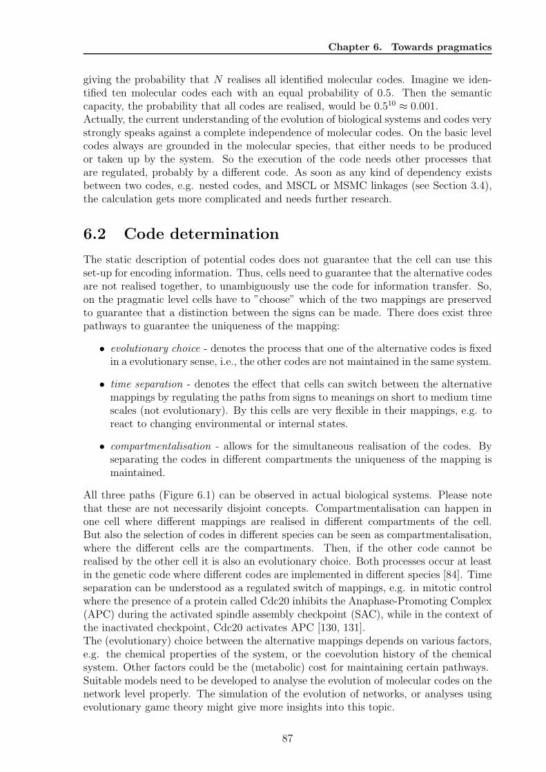
Chapter 6. Towards pragmatics
giving the probability that N realises all identified molecular codes. Imagine we iden-tified ten molecular codes each with an equal probability of 0.5. Then the semanticcapacity, the probability that all codes are realised, would be 0.510 ≈ 0.001.Actually, the current understanding of the evolution of biological systems and codes verystrongly speaks against a complete independence of molecular codes. On the basic levelcodes always are grounded in the molecular species, that either needs to be producedor taken up by the system. So the execution of the code needs other processes thatare regulated, probably by a different code. As soon as any kind of dependency existsbetween two codes, e.g. nested codes, and MSCL or MSMC linkages (see Section 3.4),the calculation gets more complicated and needs further research.
6.2 Code determination
The static description of potential codes does not guarantee that the cell can use thisset-up for encoding information. Thus, cells need to guarantee that the alternative codesare not realised together, to unambiguously use the code for information transfer. So,on the pragmatic level cells have to ”choose” which of the two mappings are preservedto guarantee that a distinction between the signs can be made. There does exist threepathways to guarantee the uniqueness of the mapping:
• evolutionary choice - denotes the process that one of the alternative codes is fixedin a evolutionary sense, i.e., the other codes are not maintained in the same system.
• time separation - denotes the effect that cells can switch between the alternativemappings by regulating the paths from signs to meanings on short to medium timescales (not evolutionary). By this cells are very flexible in their mappings, e.g. toreact to changing environmental or internal states.
• compartmentalisation - allows for the simultaneous realisation of the codes. Byseparating the codes in different compartments the uniqueness of the mapping ismaintained.
All three paths (Figure 6.1) can be observed in actual biological systems. Please notethat these are not necessarily disjoint concepts. Compartmentalisation can happen inone cell where different mappings are realised in different compartments of the cell.But also the selection of codes in different species can be seen as compartmentalisation,where the different cells are the compartments. Then, if the other code cannot berealised by the other cell it is also an evolutionary choice. Both processes occur at leastin the genetic code where different codes are implemented in different species [84]. Timeseparation can be understood as a regulated switch of mappings, e.g. in mitotic controlwhere the presence of a protein called Cdc20 inhibits the Anaphase-Promoting Complex(APC) during the activated spindle assembly checkpoint (SAC), while in the context ofthe inactivated checkpoint, Cdc20 activates APC [130, 131].The (evolutionary) choice between the alternative mappings depends on various factors,e.g. the chemical properties of the system, or the coevolution history of the chemicalsystem. Other factors could be the (metabolic) cost for maintaining certain pathways.Suitable models need to be developed to analyse the evolution of molecular codes on thenetwork level properly. The simulation of the evolution of networks, or analyses usingevolutionary game theory might give more insights into this topic.
87
6.3. Codes between system states
Figure 6.1 Illustration of the three pathways of code determination. Kineticseparation (left) leads to one of the mappings by increasing the rates of the reactionsrealising this mapping. Compartmentalisation (middle) separates the two mappingseither in compartments, or different species. Fixation (right) deletes the alternativemapping completely.
6.3 Codes between system states
In the static framework only mappings between molecular species could be detected viathe reactions of the system. Some codes can only be identified in a dynamic frame-work, as could be seen at the phosphorylation cascade example. Dynamics can be(re-)introduced to the network model via the kinetic laws of the reactions. The system’sdynamic behaviour can be concisely modelled as the solution of a system of ordinarydifferential equations. Let xt = (x1,t, x2,t, . . . , x|M|,t)
T be a vector containing the concen-trations of the system components at time point t. The systems behaviour is determinedby dxt
dt= f(xt). Using time, the network structure, and the kinetics as causal relationship
between two system states is will be possible to define a (dynamic) molecular code thatmaps from a state x(1) to a state x(2). A code, in analogy to the static code definition,is present, if under changing contexts the mapping changes. A context, here, couldbe for example the initial concentration, or the concentration level of a selected subsetof molecular species C = xc the alternative context C ′ could now be a different setof species xc′, or the same set with a different concentration vector x′c. Also dynamicswitching between mappings can be easily implemented, because the context can bepart of the system, and thus, its concentration vector can easily be influenced by thegeneral system’s behaviour (unless its an uncorrelated, separated subsystem).
The introduction of dynamics opens a huge new chapter in code biology. When systemstates can be used a signs and meanings (if the cell can read the state somehow) then themodel could also describe information transfer by dynamic behaviour, e.g. calcium os-cillations. Then mapping can also be realised between fixed points of the system, or any
88
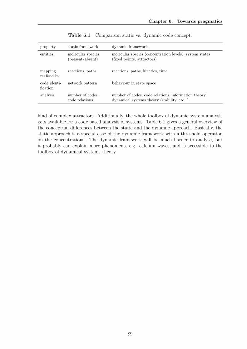
Chapter 6. Towards pragmatics
Table 6.1 Comparison static vs. dynamic code concept.
property static framework dynamic framework
entities molecular species(present/absent)
molecular species (concentration levels), system states(fixed points, attractors)
mappingrealised by
reactions, paths reactions, paths, kinetics, time
code identi-fication
network pattern behaviour in state space
analysis number of codes,code relations
number of codes, code relations, information theory,dynamical systems theory (stability, etc. )
kind of complex attractors. Additionally, the whole toolbox of dynamic system analysisgets available for a code based analysis of systems. Table 6.1 gives a general overview ofthe conceptual differences between the static and the dynamic approach. Basically, thestatic approach is a special case of the dynamic framework with a threshold operationon the concentrations. The dynamic framework will be much harder to analyse, butit probably can explain more phenomena, e.g. calcium waves, and is accessible to thetoolbox of dynamical systems theory.
89

6.3. Codes between system states
90
Chapter 7
Discussion and Outlook
I developed a formalisation of molecular codes in the context of reaction network models.This thesis covered the conceptual introduction to codes and discussed the usage of theterm code for different biological systems. I also developed different algorithms for codeidentification and presented the results of the algorithms’ application to various systems(discussed at the end of Chapter 5).Many open questions and ways to continue research in this field remain.
Improvement of algorithms The presented algorithms follow brute-force strategies.For the pathway-based algorithm I suggested two improvements, first, a parametri-sation on the K-shortest paths and, second, a Monte-Carlo type sampling algorithm.Both allow for the analysis of larger networks but in practical situations do not find allcodes. Additionally, a computational challenge remain, because the runtime complexity(number of paths, number of closed sets) leaves the feasible problem sizes quite fast.Thus a need for improved methods is still given.
Choice of network models The code based analysis of systems needs complete net-work models, i.e. the network is required to represent all possible reactions that canhappen among the molecular species and thus is a complete model of the world. In thisthesis I showed that such networks can partly be reconstructed by expert knowledge ormerge approaches. The knowledge based approach is especially necessary if the hypothe-sis that cells maintain only one of the potential mappings is true. Then, networks derivedfrom experiments cannot contain the alternative mappings, because they are invisibleto experimental techniques. If different mappings are implemented in different compart-ments a merge on the reaction networks can help to bring both realisations together inone network. This has been demonstrated in Section 5.5 for the genetic code. Datasources like the Biomodels database (http://www.ebi.ac.uk/biomodels-main/) usuallycontain only subnetworks that does not reflect the complete system, but only explain cer-tain selected subsystems. Large scale network models like KEGG or BioCyc convergetowards complete models, but may contain faulty data, even with constant curation.Additionally, a computational challenge remains, because the current algorithms cannot, or only hardly handle such large networks. The proposed heuristics (K-shortestpaths, Monte-Carlo sampling) does not guarantee to identify all codes and thus otheralternative approaches needs to be identified.Throughout the thesis it showed that slightly different models of the same chemistrycan have an effect on the results of the code based analysis. For example, the night sidemodel of Mars had codes when only taking the inflow reaction away, but no codes if
91
all reactions using light were deleted from the model. Increased detail in the networkmodels can also lead to increased semantic capacity, as for example in the network modelof the coupled GC-GRN network. The most detailed model might be best suited fora code based analysis, but will be hard to analyse. Thus, for practical applications atrade-off between level of detail and computational feasibility has to be found.
Evolution of Molecular Codes Many hypothesis have been made how the geneticcode has evolved [132, 133, 17]. Koonin [17] stated that to understand the evolution ofthe genetic code we have to understand the evolution of codes in general. The codesdefined in this paper may be suitable to understand how codes in general evolve. Aworking hypothesis emerging from the results presented in this thesis is that duringthe origin of life (chemical evolution) and the evolution of life the semantic capacityin the reaction systems discovered and incorporated by living systems increased. Abasic, but not necessarily the best, measure for semantic capacity may be the numberof BMCs as presented in this thesis. Possible other measures of semantic capacity (corecodes, probabilities) have been discussed in this thesis. The hypothesis is supported byintrinsic differences in the subsystems used by cells. For example, the metabolic systemis much more governed by the physical and chemical rules applied to the reactions (e.g.mass conservation) than the gene regulatory system whose semantic capacity is based inthe contingent combination of promoters and protein encoding DNA. Nevertheless themetabolism could be used for encoding information if cells can regulate their metabolicpathways appropriately (cp. results presented in Section 5.9.1). The validation ofthe hypothesis needs careful integration of the data and further development of thealgorithms.Also in the context of evolution of codes it can be hypothesised that cost efficient codesare preferred over more costly codes. Costs, here, can be for example measured bymetabolic costs of the paths realising a code. Tlusty [23] uses a different notion ofcosts based on the number of bits necessary to encode the transmitted information,assuming that more complex, and thus more expensive, signs are necessary for a largerinformation content. As have been shown by Tlusty a code itself has a fitness that isdetermined by its encoding properties [23]. Both notions of costs cover different aspectsof a code. While the first notion is more directly linked to the energy the cell has tospend to maintain the mapping Tlusty’s notion is more abstract on the properties ofthe signs (and meanings). Applying a fitness measure to a code, it can be understoodto be relevant also to biological fitness. Now it can be hypothesised that a biologicalspecies’ fitness depends on its capability to encode information.If codes are beneficial for a species’ fitness it can be also hypothesised that cells, inthe course of evolution, increased the number of codes. Cells may have increased theirsemantic capacity by acquiring new biochemical subsystem that allowed for encodinginformation. Proving this hypothesis needs though even more research efforts, e.g. inestablishing evolutionary game theoretical models.
Towards dynamics This work provided a first step into a deeper understanding ofcertain properties of molecular codes. The molecular code framework is well suitedto describe the mechanistic properties of molecular codes, but lacks for example thedynamic level. The analysis of phosphorylation cascades demonstrated that codes thatare based on concentration levels are not covered by the framework in the actual state.The extension to a dynamic formulation thus is one of the major research themes in this
92
Chapter 7. Discussion and Outlook
field. First steps have been made, though (cp. [80]).The extension to a dynamic framework of molecular codes integrates into already es-tablished analysis techniques and can be coupled with steady state analyses where fixedpoints or attractors are analysed. It may also prove beneficial to couple code basednetwork analysis to a Petri net formulation. Petri nets have been successfully appliedin modelling and analysis of biological networks [134, 135] and come with a well definedset of concepts for the structural and dynamical analysis that also can be linked to thenotion of molecular codes.It also needs to be checked how the code concept is related to the notion of chemicalorganisations [61]. Both concepts are related through the notion of closed sets andpotentially there exist codes between organisation. If so, then a (bio-)chemical systemcould move between its chemical organisations in an arbitrary way defined by a molecularcontext.
Relation to information theory The definition of BMCs captures some semanti-cal aspect of biological information. A common approach to information in biologicalsystems is to equate information with correlation or mutual information between tworandom sources, e.g. the message and its environment [1]. High mutual informationwould also be necessary for BMCs, but is not sufficient. In other words, measuring acorrelation or mutual information between two worlds does not necessarily imply thatthere is a code or a semiotic structure. In addition “arbitrariness” is needed, repre-sented formally by the alternative context C ′. Otherwise the mapping is based on directphysical causal relationship or a natural sign (cf.[16]).If we already know that a molecular codes exist, e.g. identified by the presented al-gorithms, the information theoretic analysis between signs and meanings can be veryinformative about the nature of the code, and perhaps also helps in validating codes.To model molecular codes in information theoretic terms signs and meanings have tobe understood as random variables, either discrete (on/off) or continuous. Then, alsocertain assumptions about the used distributions have to be made, or empirically deter-mined, if possible. For entropy measures the empirical determination might be feasible,but for mutual information, which needs the joint entropy, the non-realised associationsmight never be measurable. Here only reasonable estimates can help.
Simulation environment The analysis of the pragmatic level of molecular codes canbe implemented in the simulation framework ArtBact developed by Erbach [136] andWeisensee [137]. ArtBact allows for the evolution of cellular networks. Thus, it is wellsuited to tackle questions related to the structural evolution of molecular codes underdefined environmental conditions.More concretely, I suggest to perform an evolution experiment with two external chemoat-tractants, or other kind of signals. The bacterium contains two kinds of effector andshould learn to transduce information about the external signal concentration via itsregulatory networks to the effectors. The fitness in such an experiment can be a com-bination of biomass, i.e. the bacteria learn to survive, and, in a first step, the exclusiveusage of one of the effectors. By this strong constraint we might be able to learn whatkind of networks evolve to reach optimal fitness values. In particular, it might be inter-esting to see whether network structures similar to the formalisation of codes evolves,or if different approaches, e.g. by dynamic behaviour, get visible to get a higher fitness.The ArtBact framework allows to apply information theoretic measures like mutual
93
information to the generated time series data. This links the structural definition ofmolecular codes to dynamics and thus enter the pragmatic level.
Experimental validation Finally, the notion of codes directly generates input forpotential wet-lab experiments. The codes identified in network models of a certainsystem can be checked by experiments that follow the closure algorithm. For a proposedmolecular code the experiment needs to check whether for the two signs combined withthe two contexts, independently, the two meanings are produced. The experimentalvalidation of molecular codes is the best possible type of validation, because in-vivo thepragmatic dynamic level is always present and thus non-feasible codes can be identifiedexactly.Overall, I presented a theoretical framework and demonstrated applications to variousnetwork models. As outlined in this chapter, the definitions with respect to chemicalreaction networks opened the door to many new research questions that needs to beanswered in future studies.
94
References
[1] C. Waltermann, E. Klipp (2011) Information theory based approaches to cellularsignaling. Biochim Biophys Acta, 1810(10):924–932.
[2] T. Kohler, G. G. Perron, A. Buckling, C. van Delden (2010) Quorum sensinginhibition selects for virulence and cooperation in pseudomonas aeruginosa. PLoSPathog, 6(5):e1000883.
[3] C. E. Shannon (1948) A mathematical theory of communication. The Bell Sys-tems Technical Journal, 27:379–423, 623–656.
[4] G. Tkacik, A. M. Walczak (2011) Information transmission in genetic regulatorynetworks: a review. J Phys Condens Matter, 23(15):153102.
[5] P. Mehta, S. Goyal, T. Long, B. L. Bassler, N. S. Wingreen (2009) Informationprocessing and signal integration in bacterial quorum sensing. Mol Syst Biol,5:325. (doi:10.1038/msb.2009.79).
[6] T. Lenaerts, J. Ferkinghoff-Borg, F. Stricher, L. Serrano, J. W. H. Schymkowitz,F. Rousseau (2008) Quantifying information transfer by protein domains: analysisof the Fyn SH2 domain structure. BMC Struct Biol, 8:43.
[7] J. Monod (1971) Chance and necessity. Alfred Knopf, New York/NY. (Originallypublished 1970).
[8] B.-O. Kuppers (1990) Information and the origin of life. MIT Press, Cam-bridge/MA. (Originally published 1986).
[9] C. Morris (1971) Writing on the general theory of signs. Mouton, Den Haag.
[10] P. Bralley (1996) An introduction to molecular linguistics. BioScience, 46(2):146–153.
[11] M. Gimona (2006) Protein linguistics - a grammar for modular protein assembly?Nat Rev Mol Cell Biol, 7(1):68–73.
[12] S. Artmann (2008) Biological information. In S. Sarkar, A. Plutynski (eds.),A companion to the philosophy of biology, no. 39 in Blackwell companions tophilosophy, chap. 2, 22–39. Blackwell Publishing.
[13] A. Jayaraman, T. K. Wood (2008) Bacterial quorum sensing: Signals, circuits,and implications for biofilms and disease. Annu Rev Biomed Eng, 10:145–167.
95
References
[14] S. Artmann (2007) Computing codes versus interpreting life: Two alternativeways of synthesizing biological knowledge through semantics. In M. Barbieri (ed.),Introduction to biosemiotics: The new biological synthesis, 209–233. Dodrecht:Springer.
[15] D. Chandler (2007) Semiotics: the basics. Routledge, Abingdon, UK, 2nd edn.
[16] M. Barbieri (2008) Biosemiotics: a new understanding of life. Naturwis-senschaften, 95(7):577–599.
[17] E. V. Koonin, A. S. Novozhilov (2009) Origin and evolution of the genetic code:the universal enigma. IUBMB Life, 61(2):99–111.
[18] S. Artmann (2002) Three types of semiotic indeterminacy in monod’s philosophyof modern biology. Sign System Studies, 30(1):149–169.
[19] H. H. Pattee (2008) Physical and functional conditions for symbols, codes, andlanguages. Biosemiotics, 1(2):147–168.
[20] J. Maynard Smith (2000) The concept of information in biology. Philosophy ofscience, 67:177–194.
[21] S. Sarkar (2000) Information in Genetics and Developmental Biology: Commentson Maynard Smith. Philosophy of Science, 67:208–213.
[22] U. Stegmann (2004) The arbitrariness of the genetic code. Biology & Philosophy,19(2):205–222.
[23] T. Tlusty (2008) Casting polymer nets to optimize noisy molecular codes. ProcNatl Acad Sci U S A, 105(24):8238–8243.
[24] J. Bierbrauer (2005) Introduction to coding theory. Discrete Mathematics and itsapplications. Chapman & Hall/CRC, Boca Raton, Fl.
[25] T. M. Cover, J. A. Thomas (1991) Elements of Information Theory. Wiley seriesin telecommunications. Wiley, New York, NY.
[26] S. Verdu (1998) Fifty years of Shannon theory. IEEETransactions on InformationTheory, 44(6):2057–2078.
[27] D. J. MacKay (2003) Information Theory, Inference, and Learning Algorithms.Cambridge University Press.
[28] T. Tlusty (2008) A simple model for the evolution of molecular codes driven bythe interplay of accuracy, diversity and cost. Phys Biol, 5(1):16001.
[29] T. Tlusty (2008) Rate-distortion scenario for the emergence and evolution of noisymolecular codes. Phys Rev Lett, 100(4):048101.
[30] K. Vetsigian, C. Woese, N. Goldenfeld (2006) Collective evolution and the geneticcode. Proc Natl Acad Sci U S A, 103(28):10696–10701.
[31] M. Barbieri (2003) The organic codes: An introduction to semantic biology. Cam-bridge University Press, Cambridge.
96
References
[32] D. Gorlich, S. Artmann, P. Dittrich (2011) Cells as semantic systems. BiochimBiophys Acta, 1810(10):914–923.
[33] M. G. Safro, N. A. Moor (2009) Codases: fifty years after. Mol Biol (Mosk),43(2):230–242.
[34] L. L. Kiselev (1990) Aminoacyl-tRNA synthetases (codases) and their noncanon-ical functions. Mol Biol (Mosk), 24(6):1445–1473.
[35] D. Schwarzer (2010) Chemical tools in chromatin research. J Pept Sci, 16(10):530–537.
[36] J.-S. Lee, E. Smith, A. Shilatifard (2010) The language of histone crosstalk. Cell,142(5):682–685.
[37] S. J. Prohaska, P. F. Stadler, D. C. Krakauer (2010) Innovation in gene regulation:the case of chromatin computation. J Theor Biol, 265(1):27–44.
[38] A. Csordas (1990) On the biological role of histone acetylation. Biochem J,265(1):23–38.
[39] B. M. Turner (1993) Decoding the nucleosome. Cell, 75(1):5–8.
[40] B. M. Turner (2000) Histone acetylation and an epigenetic code. Bioessays,22(9):836–845.
[41] B. D. Strahl, C. D. Allis (2000) The language of covalent histone modifications.Nature, 403(6765):41–45.
[42] T. Jenuwein, C. D. Allis (2001) Translating the histone code. Science,293(5532):1074–1080.
[43] K. A. Gelato, W. Fischle (2008) Role of histone modifications in defining chro-matin structure and function. Biol Chem, 389(4):353–363.
[44] A. Lennartsson, K. Ekwall (2009) Histone modification patterns and epigeneticcodes. Biochim Biophys Acta, 1790(9):863–868.
[45] B. M. Turner (2002) Cellular memory and the histone code. Cell, 111(3):285–291.
[46] S. Henikoff (2005) Histone modifications: combinatorial complexity or cumulativesimplicity? Proc Natl Acad Sci U S A, 102(15):5308–5309.
[47] M. F. Dion, S. J. Altschuler, L. F. Wu, O. J. Rando (2005) Genomic character-ization reveals a simple histone H4 acetylation code. Proc Natl Acad Sci U S A,102(15):5501–5506.
[48] R. Margueron, P. Trojer, D. Reinberg (2005) The key to development: interpret-ing the histone code? Curr Opin Genet Dev, 15(2):163–176.
[49] J. Moriniere, S. Rousseaux, U. Steuerwald, M. Soler-Lopez, S. Curtet, A.-L. Vitte,J. Govin, J. Gaucher, K. Sadoul, D. J. Hart, J. Krijgsveld, S. Khochbin, C. W.Muller, C. Petosa (2009) Cooperative binding of two acetylation marks on ahistone tail by a single bromodomain. Nature, 461(7264):664–668.
97
References
[50] J. I. Wu, J. Lessard, G. R. Crabtree (2009) Understanding the words of chromatinregulation. Cell, 136(2):200–206.
[51] H.-J. Gabius (2000) Biological information transfer beyond the genetic code: thesugar code. Naturwissenschaften, 87(3):108–121.
[52] H.-J. Gabius, S. Andre, H. Kaltner, H.-C. Siebert (2002) The sugar code: func-tional lectinomics. Biochim Biophys Acta, 1572(2-3):165–177.
[53] H.-J. Gabius (ed.) (2009) The sugar code: Fundamentals of glycosciences. Wiley-VCH, Weinheim.
[54] H. Rudiger, H.-J. Gabius (2009) The sugar code: Fundamentals of glycosciences,chap. The biochemical basis and coding capacity of the sugar code, 3–13. Wiley-VCH.
[55] R. Laine (1997) The information-storing potential of the sugar code. In H.-J.Gabius (ed.), Glycosciences: Status and Perspectives. Chapman & Hall, London.
[56] J. Holgersson, A. Gustafsson, S. Gaunitz (2009) The sugar code: Fundamentals ofglycosciences, chap. Bacterial and viral lectins, 279–300. Wiley-VCH, Weinheim.
[57] H. Rudiger, H.-J. Gabius (2009) The sugar code: Fundamentals of glycosciences,chap. Plant lectins, 301–315. Wiley-VCH, Weinheim.
[58] H.-J. Gabius (2009) The sugar code: Fundamentals of glycosciences, chap. Animaland human lectines, 317–328. Wiley-VCH.
[59] N. Sharon, H. Lis (1989) Lectins as cell recognition molecules. Science,246(4927):227–234.
[60] D. Gorlich, P. Dittrich (2011) Identifying molecular organic codes in reactionnetworks. In G. Kampis, I. Karsai, E. Szathmary (eds.), Advances in ArtificialLife. Darwin Meets von Neumann, vol. 5777 of Lecture Notes in Computer Science,305–312. Springer Berlin / Heidelberg.
[61] P. Dittrich, P. S. D. Fenizio (2007) Chemical organization theory. Bull Math Bio,69(3):1199–1231.
[62] W. Fontana, L. W. Buss (1994) The arrival of the fittest: Toward a theory ofbiological organization. Bull Math Bio, 56:1–64.
[63] C. Meinel, M. Mundhenk (2002) Mathematische Grundlagen der Informatik.Teubner B.G. GmbH.
[64] M. Hucka, A. Finney, H. M. Sauro, H. Bolouri, J. C. Doyle, H. Kitano, A. P.Arkin, B. J. Bornstein, D. Bray, A. Cornish-Bowden, A. A. Cuellar, S. Dronov,E. D. Gilles, M. Ginkel, V. Gor, I. I. Goryanin, W. J. Hedley, T. C. Hodgman,J.-H. Hofmeyr, P. J. Hunter, N. S. Juty, J. L. Kasberger, A. Kremling, U. Kum-mer, N. L. Novere, L. M. Loew, D. Lucio, P. Mendes, E. Minch, E. D. Mjolsness,Y. Nakayama, M. R. Nelson, P. F. Nielsen, T. Sakurada, J. C. Schaff, B. E.Shapiro, T. S. Shimizu, H. D. Spence, J. Stelling, K. Takahashi, M. Tomita,
98
References
J. Wagner, J. Wang, S. B. M. L. Forum (2003) The systems biology markup lan-guage (sbml): a medium for representation and exchange of biochemical networkmodels. Bioinformatics, 19(4):524–531.
[65] A. Finney, M. Hucka (2003) Systems biology markup language: Level 2 andbeyond. Biochem Soc Trans, 31(Pt 6):1472–1473.
[66] B. Roberts, D. P. Kroese (2007) Estimating the number of s-t paths in a graph.Journal of Graph Algorithms and Applications, 11(1):195–214.
[67] J. Y. Yen (1971) Finding the K shortest loopless paths in a network. Managementscience, 17:712–716.
[68] D. Eppstein (1998) Finding the k shortest paths. SIAM J on Computing,28(2):652–673.
[69] F. J. Planes, J. E. Beasley (2008) A critical examination of stoichiometric andpath-finding approaches to metabolic pathways. Brief Bioinform, 9(5):422–436.
[70] E. Q. V. Martins, M. M. B. Pascoal (2003) A new implementation of yen’s rank-ing loopless paths algorithm. 4OR: A Quarterly Journal of Operations Research,1:121–133. 10.1007/s10288-002-0010-2.
[71] E. Kaiser, T. Wallington, M. D. Hurley, J. Platz, H. J. Curran, W. J. Pitz, C. K.Westbrook (2000) Experimental and modeling study of premixed atmospheric-pressure dimethyl ether-air flames. J Phys Chem A, 104(35):8194–8206.
[72] N. M. Marinov (1999) A detailed chemical kinetic model for high temperatureethanol oxidation. Int J Chem Kinet, 31:183–220.
[73] M. O. Conaire, H. J. Curran, J. M. Simmie, W. J. Pitz, C. Westbrook (2004)A comprehensive modeling study of hydrogen oxidation. Int J Chem Kinet,36(11):603–622.
[74] T. Turnyi, K. Hughes, M. Pilling, A. Tomlin (2001). The Leedsmethane oxidation mechanism. online. Version 1.5, available athttp://www.chem.leeds.ac.uk/Combustion/methane.htm.
[75] W. Banzhaf (1993) Self-replicating sequences of binary numbers. Comput MathAppl, 26:1–8.
[76] H. Nair, M. Allen, A. D. Anbar, Y. L. Yung (1994) A photochemical model ofthe martian athmosphere. Icarus, 111:124–150.
[77] F. Centler, P. Dittrich (2007) Chemical organizations in atmospheric photo-chemistries: a new method to analyze chemical reaction networks. Planet SpaceSci, 55(4):413–428.
[78] F. Centler (2008) Chemical organizations in natural reaction networks. Ph.D.thesis, Friedrich-Schiller-Universitat Jena.
[79] F. H. Crick, L. Barnett, S. Brenner, R. J. Watts-Tobin (1961) General nature ofthe genetic code for proteins. Nature, 192:1227–1232.
99
References
[80] J. DeBeule, E. Hovig, M. Benson (2010) Introducing dynamics into the field ofbiosemiotics. Biosemiotics, 4:5–24.
[81] R. Knippers (2006) Molekulare Genetik. Georg Thieme Verlag, Stuttgart, 9 edn.In German.
[82] S. Osawa, T. H. Jukes, K. Watanabe, A. Muto (1992) Recent evidence for evolu-tion of the genetic code. Microbiol Rev, 56(1):229–264.
[83] T. H. Jukes, S. Osawa (1993) Evolutionary changes in the genetic code. CompBiochem Physiol B, 106(3):489–494.
[84] A. Elzanowski, J. Ostell (2010). The genetic code. Last update: July 7, 2010.Retrieved: March 1, 2011.URL http://www.ncbi.nlm.nih.gov/Taxonomy/Utils/wprintgc.cgi
[85] M. Di Giulio (2008) An extension of the coevolution theory of the origin of thegenetic code. Biol Direct, 3:37.
[86] G. D. Clark-Walker, G. F. Weiller (1994) The structure of the small mitochondrialDNA of Kluyveromyces thermotolerans is likely to reflect the ancestral gene orderin fungi. J Mol Evol, 38(6):593–601.
[87] H. Himeno, H. Masaki, T. Kawai, T. Ohta, I. Kumagai, K. Miura, K. Watanabe(1987) Unusual genetic codes and a novel gene structure for tRNA(AGYSer) instarfish mitochondrial DNA. Gene, 56(2-3):219–230.
[88] H. T. Jacobs, D. J. Elliott, V. B. Math, A. Farquharson (1988) Nucleotide se-quence and gene organization of sea urchin mitochondrial DNA. J Mol Biol,202(2):185–217.
[89] B. Batuecas, R. Garesse, M. Calleja, J. R. Valverde, R. Marco (1988) Genomeorganization of Artemia mitochondrial DNA. Nucleic Acids Res, 16(14A):6515–6529.
[90] S. Osawa, T. Ohama, T. H. Jukes, K. Watanabe (1989) Evolution of the mi-tochondrial genetic code. I. origin of AGR serine and stop codons in metazoanmitochondria. J Mol Evol, 29(3):202–207.
[91] J. R. Garey, D. R. Wolstenholme (1989) Platyhelminth mitochondrial DNA: evi-dence for early evolutionary origin of a tRNA(serAGN) that contains a dihydrouri-dine arm replacement loop, and of serine-specifying AGA and AGG codons. J MolEvol, 28(5):374–387.
[92] T. Ohama, S. Osawa, K. Watanabe, T. H. Jukes (1990) Evolution of the mitochon-drial genetic code. IV. AAA as an asparagine codon in some animal mitochondria.J Mol Evol, 30(4):329–332.
[93] R. J. Hoffmann, J. L. Boore, W. M. Brown (1992) A novel mitochondrial genomeorganization for the blue mussel, Mytilus edulis. Genetics, 131(2):397–412.
100
References
[94] G. A. Durrheim, V. A. Corfield, E. H. Harley, M. H. Ricketts (1993) Nucleotidesequence of cytochrome oxidase (subunit III) from the mitochondrion of the tu-nicate Pyura stolonifera: evidence that AGR encodes glycine. Nucleic Acids Res,21(15):3587–3588.
[95] J. L. Boore, W. M. Brown (1994) Complete DNA sequence of the mitochondrialgenome of the black chiton, Katharina tunicata. Genetics, 138(2):423–443.
[96] A. Kondow, T. Suzuki, S. Yokobori, T. Ueda, K. Watanabe (1999) An extratRNAGly(U*CU) found in ascidian mitochondria responsible for decoding non-universal codons AGA/AGG as glycine. Nucleic Acids Res, 27(12):2554–9.
[97] M. J. Telford, E. A. Herniou, R. B. Russell, D. T. Littlewood (2000) Changesin mitochondrial genetic codes as phylogenetic characters: two examples from theflatworms. Proc Natl Acad Sci U S A, 97(21):11359–11364.
[98] S. Yokobori, Y. Watanabe, T. Oshima (2003) Mitochondrial genome of Cionasavignyi (Urochordata, Ascidiacea, Enterogona): comparison of gene arrangementand tRNA genes with Halocynthia roretzi mitochondrial genome. J Mol Evol,57(5):574–587.
[99] A. M. Nedelcu, R. W. Lee, C. Lemieux, M. W. Gray, G. Burger (2000) Thecomplete mitochondrial DNA sequence of Scenedesmus obliquus reflects an inter-mediate stage in the evolution of the green algal mitochondrial genome. GenomeRes, 10(6):819–831.
[100] Y. Hayashi-Ishimaru, T. Ohama, Y. Kawatsu, K. Nakamura, S. Osawa (1996)UAG is a sense codon in several chlorophycean mitochondria. Curr Genet,30(1):29–33.
[101] M. J. Laforest, I. Roewer, B. F. Lang (1997) Mitochondrial tRNAs in the lowerfungus Spizellomyces punctatus: tRNA editing and UAG ’stop’ codons recognizedas leucine.· . Nucleic Acids Res, 25(3):626–632.
[102] S. U. Schneider, M. B. Leible, X. P. Yang (1989) Strong homology between thesmall subunit of ribulose-1,5-bisphosphate carboxylase/oxygenase of two speciesof Acetabularia and the occurrence of unusual codon usage. Mol Gen Genet,218(3):445–452.
[103] S. U. Schneider, E. J. de Groot (1991) Sequences of two rbcS cDNA clones ofBatophora oerstedii: structural and evolutionary considerations. Curr Genet,20(1-2):173–175.
[104] A. Liang, K. Heckmann (1993) Blepharisma uses UAA as a termination codon.Naturwissenschaften, 80(5):225–226.
[105] P. J. Keeling, W. F. Doolittle (1996) A non-canonical genetic code in an earlydiverging eukaryotic lineage. EMBO J, 15(9):2285–2290.
[106] A. Kaufmann, M. Knop (2011) Genomic promoter replacement cassettes to altergene expression in the yeast saccharomyces cerevisiae. Methods Mol Biol, 765:275–294.
101
References
[107] A. A. Brakhage, V. Schroeckh (2011) Fungal secondary metabolites - strategiesto activate silent gene clusters. Fungal Genet Biol, 48(1):15–22.
[108] M. Kanehisa, S. Goto (2000) KEGG: kyoto encyclopedia of genes and genomes.Nucleic Acids Res, 28(1):27–30.
[109] M. Kanehisa, S. Goto, Y. Sato, M. Furumichi, M. Tanabe (2012) KEGG forintegration and interpretation of large-scale molecular data sets. Nucleic AcidsRes, 40(Database issue):D109–D114.
[110] R. B. Weart, A. H. Lee, A.-C. Chien, D. P. Haeusser, N. S. Hill, P. A. Levin(2007) A metabolic sensor governing cell size in bacteria. Cell, 130(2):335–347.
[111] G. Krauss (2008) Biochemistry of Signal Transduction and Regulation. Wiley-VCH, Weinheim, 4 edn.
[112] R. Avraham, Y. Yarden (2011) Feedback regulation of EGFR signalling: decisionmaking by early and delayed loops. Nat Rev Mol Cell Biol, 12(2):104–117.
[113] A. R. Saltiel, C. R. Kahn (2001) Insulin signalling and the regulation of glucoseand lipid metabolism. Nature, 414(6865):799–806.
[114] L. F. Reichardt (2006) Neurotrophin-regulated signalling pathways. Philos TransR Soc Lond B Biol Sci, 361(1473):1545–1564.
[115] J. Andrae, R. Gallini, C. Betsholtz (2008) Role of platelet-derived growth factorsin physiology and medicine. Genes Dev, 22(10):1276–1312.
[116] K. Xie, D. Wei, Q. Shi, S. Huang (2004) Constitutive and inducible expressionand regulation of vascular endothelial growth factor. Cytokine Growth Factor Rev,15(5):297–324.
[117] C. E. Edling, B. Hallberg (2007) c-Kit–a hematopoietic cell essential receptortyrosine kinase. Int J Biochem Cell Biol, 39(11):1995–1998.
[118] R. L. Patterson, D. B. van Rossum, N. Nikolaidis, D. L. Gill, S. H. Snyder (2005)Phospholipase C-gamma: diverse roles in receptor-mediated calcium signaling.Trends Biochem Sci, 30(12):688–697.
[119] B. D. Manning, L. C. Cantley (2007) AKT/PKB signaling: navigating down-stream. Cell, 129(7):1261–1274.
[120] M. M. McKay, D. K. Morrison (2007) Integrating signals from RTKs toERK/MAPK. Oncogene, 26(22):3113–3121.
[121] A. B. Jaffe, A. Hall (2005) Rho GTPases: biochemistry and biology. Annu RevCell Dev Biol, 21:247–269.
[122] D. Chen, M. Zhao, G. R. Mundy (2004) Bone morphogenetic proteins. GrowthFactors, 22(4):233–241.
[123] J. S. Kang, C. Liu, R. Derynck (2009) New regulatory mechanisms of TGF-betareceptor function. Trends Cell Biol, 19(8):385–394.
102
References
[124] W. M. Oldham, H. E. Hamm (2008) Heterotrimeric G protein activation by G-protein-coupled receptors. Nat Rev Mol Cell Biol, 9(1):60–71.
[125] B. T. MacDonald, K. Tamai, X. He (2009) Wnt/beta-catenin signaling: compo-nents, mechanisms, and diseases. Dev Cell, 17(1):9–26.
[126] D. Pan (2010) The hippo signaling pathway in development and cancer. Dev Cell,19(4):491–505.
[127] M. A. Arnaout, S. L. Goodman, J.-P. Xiong (2002) Coming to grips with integrinbinding to ligands. Curr Opin Cell Biol, 14(5):641–651.
[128] L. Matthews, G. Gopinath, M. Gillespie, M. Caudy, D. Croft, B. de Bono, P. Gara-pati, J. Hemish, H. Hermjakob, B. Jassal, A. Kanapin, S. Lewis, S. Mahajan,B. May, E. Schmidt, I. Vastrik, G. Wu, E. Birney, L. Stein, P. D’Eustachio (2009)Reactome knowledgebase of human biological pathways and processes. NucleicAcids Res, 37(Database issue):D619–D622.
[129] M. Barbieri (2009) Three types of semiosis. Biosemiotics, 2(1):19–30.
[130] A. Musacchio, E. D. Salmon (2007) The spindle-assembly checkpoint in spaceand time. Nat Rev Mol Cell Biol, 8(5):379–393.
[131] B. Ibrahim, S. Diekmann, E. Schmitt, P. Dittrich (2008) In-silico modeling of themitotic spindle assembly checkpoint. PLoS One, 3(2):e1555.
[132] E. Szathmary (1993) Coding coenzyme handles: a hypothesis for the origin of thegenetic code. Proc Natl Acad Sci U S A, 90:9916–9920.
[133] M. Yarus, J. G. Caporaso, R. Knight (2005) Origins of the genetic code: theescaped triplet theory. Annu Rev Biochem, 74:179–198.
[134] L. Popova-Zeugmann, M. Heiner, I. Koch (2005) Time petri net for modellingand analysis of biochemical networks. Fundamenta Informaticae, 67:149–162.
[135] M. Heiner, A. Uhrmacher (eds.) (2011) Foundations of formal reconstructionofbiochemical networks, vol. 412 of J Theoretical Computer Science.
[136] E. zu Erbach-Schonberg (2009) Simulating the evolution of signalling networks inartificial bacteria. Diploma thesis, Friedrich-Schiller-Universitat Jena.
[137] C. Weisensee (2011) Simulation of the evolution of chemotaxis in virtual cells.Diploma thesis, Friedrich-Schiller-Universitat Jena. In German.
103

References
104
List of Tables
2.1 A possible binary sugar code. . . . . . . . . . . . . . . . . . . . . . . . . 20
4.1 Empirical running time analysis. . . . . . . . . . . . . . . . . . . . . . . . 434.2 Table of predicted BMCs by code completion. . . . . . . . . . . . . . . . 48
5.1 Summary of the statistical models. . . . . . . . . . . . . . . . . . . . . . 555.2 Overview of the analysed combustion chemistries. . . . . . . . . . . . . . 585.3 Light consuming reactions in the Mars photochemistry. . . . . . . . . . . 615.4 Definition of the gene translation chemistry with synthetases. . . . . . . . 635.5 Molecular codes in the known genetic codes. . . . . . . . . . . . . . . . . 645.6 Code pairs in the gene translation model. . . . . . . . . . . . . . . . . . . 645.7 Molecular contexts of the codes in the gene translation model. . . . . . . 645.8 Codes identified in the combined GC-GRN network. . . . . . . . . . . . . 695.9 Codes identified in the extended GC-GRN network. . . . . . . . . . . . . 705.10 Contingency table of biological roles of participating molecular species. . 795.11 Number of codes per semiotic role for the biological roles. . . . . . . . . . 805.12 Combinations of biological roles occurring together in codes. . . . . . . . 815.13 Semantic roles in the analysed biological systems. . . . . . . . . . . . . . 83
6.1 Comparison static vs. dynamic code concept. . . . . . . . . . . . . . . . 89
C.1 Potential signs and meanings in human signal transduction. . . . . . . . 120
D.1 Potential codes in metabolism. . . . . . . . . . . . . . . . . . . . . . . . . 128D.2 Components of potential codes in metabolism. . . . . . . . . . . . . . . . 129
105

List of Tables
106
List of Figures
1.1 Shannon’s communication model. . . . . . . . . . . . . . . . . . . . . . . 121.2 Molecular code framework by Tlusty. . . . . . . . . . . . . . . . . . . . . 14
2.1 Model of a possible sugar code. . . . . . . . . . . . . . . . . . . . . . . . 20
3.1 Example networks with binary molecular codes. . . . . . . . . . . . . . . 273.2 Decomposition of a molecular code into binary molecular codes. . . . . . 283.3 Subsets of transitive nested BMCs. . . . . . . . . . . . . . . . . . . . . . 323.4 Reaction network with nested molecular codes. . . . . . . . . . . . . . . . 333.5 Core code relation network of Fig. 3.4 . . . . . . . . . . . . . . . . . . . 343.6 Exemplary MCSL network. . . . . . . . . . . . . . . . . . . . . . . . . . 35
4.1 Parameter scan of the random subnetwork sampling algorithm. . . . . . . 464.2 Comparison of complete and incomplete BMC. . . . . . . . . . . . . . . . 474.3 Result of the code completion algorithm on the complete BMC network. 484.4 Result of the code completion algorithm on an incomplete BMC network. 48
5.1 Code based analysis of random networks. . . . . . . . . . . . . . . . . . . 505.2 Mean number of reactions of the random network data. . . . . . . . . . . 535.3 Variances of the random network data. . . . . . . . . . . . . . . . . . . . 545.4 Empirically determined scaling factors. . . . . . . . . . . . . . . . . . . . 55
(a) N . . . . . . . . . . . . . . . . . . . . . . . . . . . . . . . . . . . . 55(b) lnN . . . . . . . . . . . . . . . . . . . . . . . . . . . . . . . . . . . 55(c) Γ . . . . . . . . . . . . . . . . . . . . . . . . . . . . . . . . . . . . . 55
5.5 Goodness of fit of random network models. . . . . . . . . . . . . . . . . . 565.6 Data and gamma model overlay. . . . . . . . . . . . . . . . . . . . . . . . 575.7 Prediction of the statistical null model. . . . . . . . . . . . . . . . . . . . 575.8 Codes in the artificial chemistry NTOP. . . . . . . . . . . . . . . . . . . 595.9 Semantic capacity of NTOP under increased randomisation. . . . . . . . 605.10 Subnetwork of the gene translation network model. . . . . . . . . . . . . 655.11 Construction of a gene regulatory network model. . . . . . . . . . . . . . 675.14 Nested codes in GC-GRN models. . . . . . . . . . . . . . . . . . . . . . . 71
(a) Simple model . . . . . . . . . . . . . . . . . . . . . . . . . . . . . . 71(b) Extended model . . . . . . . . . . . . . . . . . . . . . . . . . . . . 71
5.15 Reaction networks describing phosphorylation motifs. . . . . . . . . . . . 755.16 Map of the metabolic network. . . . . . . . . . . . . . . . . . . . . . . . . 775.17 Reaction network of the human signal transduction. . . . . . . . . . . . . 785.18 A system of codes emerging from code linkages. . . . . . . . . . . . . . . 84
6.1 Illustration of the three paths of code determination. . . . . . . . . . . . 88
107

List of Figures
108
List of Algorithms
4.1 closureCodeFinder(N) . . . . . . . . . . . . . . . . . . . . . . . . . . 394.2 pathCodeFinder(N) . . . . . . . . . . . . . . . . . . . . . . . . . . . . 404.3 MonteCarloCodeSearch(N,n,K) . . . . . . . . . . . . . . . . . . . . 444.4 expand(N,m) . . . . . . . . . . . . . . . . . . . . . . . . . . . . . . . . . 45A.1 random(x,y) . . . . . . . . . . . . . . . . . . . . . . . . . . . . . . . . . 111A.2 generateRandomNetwork() . . . . . . . . . . . . . . . . . . . . . . 111A.3 allClosedSets(A) . . . . . . . . . . . . . . . . . . . . . . . . . . . . . 112A.4 findClosAbove(A,B) . . . . . . . . . . . . . . . . . . . . . . . . . . . . 112A.5 GCL(A) . . . . . . . . . . . . . . . . . . . . . . . . . . . . . . . . . . . . . 112A.6 sqr(A,N) . . . . . . . . . . . . . . . . . . . . . . . . . . . . . . . . . . . 113A.7 getContext(p,s,t,N) . . . . . . . . . . . . . . . . . . . . . . . . . . . . 113A.8 getOutgoingRea(A,N) . . . . . . . . . . . . . . . . . . . . . . . . . . 113A.9 getIncomingRea(A,N) . . . . . . . . . . . . . . . . . . . . . . . . . . . 114A.10 getSpecies(R,N) . . . . . . . . . . . . . . . . . . . . . . . . . . . . . . 114A.11 getReactions(R,N) . . . . . . . . . . . . . . . . . . . . . . . . . . . . 114A.12 fitModel(data,dist) . . . . . . . . . . . . . . . . . . . . . . . . . . . . . 115
109

List of Algorithms
110
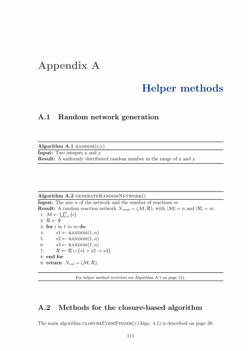
Appendix A
Helper methods
A.1 Random network generation
Algorithm A.1 random(x,y)
Input: Two integers x and y.Result: A uniformly distributed random number in the range of x and y.
Algorithm A.2 generateRandomNetwork()
Input: The size n of the network and the number of reactions mResult: A random reaction network Nrand = (M,R), with |M| = n and |R| = m.1: M← ⋃m
i=1{i}2: R ← ∅3: for i in 1 to m do4: s1← random(1, n)5: s2← random(1, n)6: s3← random(1, n)7: R ← R∪ {s1 + s2→ s3}8: end for9: return Nrea = (M,R)
For helper method random see Algorithm A.1 on page 111.
A.2 Methods for the closure-based algorithm
The main algorithm closureCodeFinder() (Algo. 4.1) is described on page 39.
111
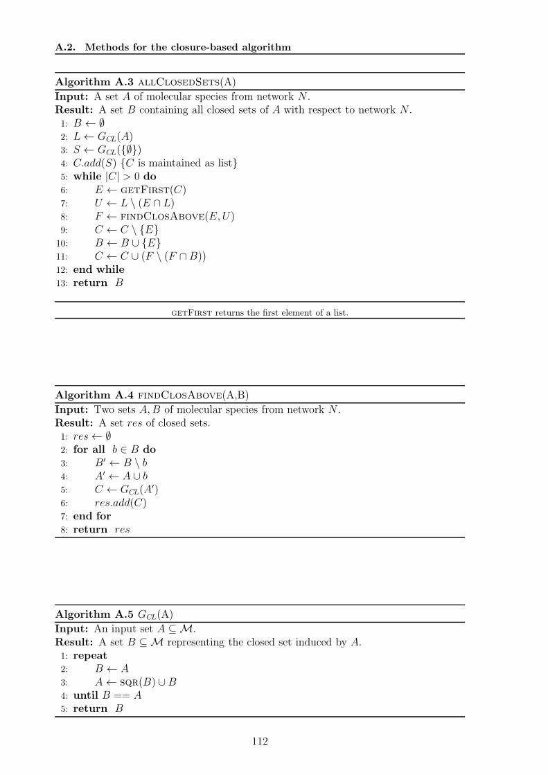
A.2. Methods for the closure-based algorithm
Algorithm A.3 allClosedSets(A)
Input: A set A of molecular species from network N .Result: A set B containing all closed sets of A with respect to network N .1: B ← ∅2: L← GCL(A)3: S ← GCL({∅})4: C.add(S) {C is maintained as list}5: while |C| > 0 do6: E ← getFirst(C)7: U ← L \ (E ∩ L)8: F ← findClosAbove(E,U)9: C ← C \ {E}
10: B ← B ∪ {E}11: C ← C ∪ (F \ (F ∩ B))12: end while13: return B
getFirst returns the first element of a list.
Algorithm A.4 findClosAbove(A,B)
Input: Two sets A,B of molecular species from network N .Result: A set res of closed sets.1: res← ∅2: for all b ∈ B do3: B′ ← B \ b4: A′ ← A ∪ b5: C ← GCL(A
′)6: res.add(C)7: end for8: return res
Algorithm A.5 GCL(A)
Input: An input set A ⊆M.Result: A set B ⊆M representing the closed set induced by A.1: repeat2: B ← A3: A← sqr(B) ∪ B4: until B == A5: return B
112
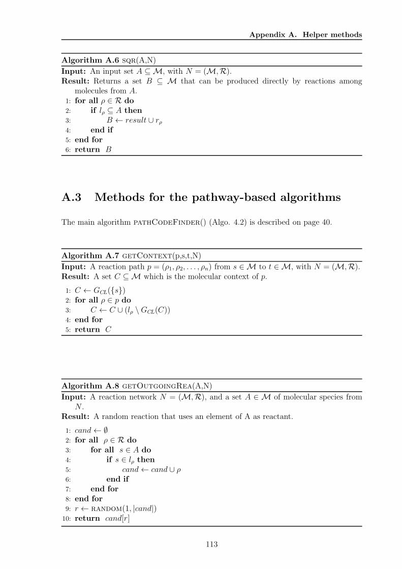
Appendix A. Helper methods
Algorithm A.6 sqr(A,N)
Input: An input set A ⊆M, with N = (M,R).Result: Returns a set B ⊆ M that can be produced directly by reactions among
molecules from A.1: for all ρ ∈ R do2: if lρ ⊆ A then3: B ← result ∪ rρ4: end if5: end for6: return B
A.3 Methods for the pathway-based algorithms
The main algorithm pathCodeFinder() (Algo. 4.2) is described on page 40.
Algorithm A.7 getContext(p,s,t,N)
Input: A reaction path p = (ρ1, ρ2, . . . , ρn) from s ∈M to t ∈M, with N = (M,R).Result: A set C ⊆M which is the molecular context of p.
1: C ← GCL({s})2: for all ρ ∈ p do3: C ← C ∪ (lρ \GCL(C))4: end for5: return C
Algorithm A.8 getOutgoingRea(A,N)
Input: A reaction network N = (M,R), and a set A ∈ M of molecular species fromN .
Result: A random reaction that uses an element of A as reactant.
1: cand← ∅2: for all ρ ∈ R do3: for all s ∈ A do4: if s ∈ lρ then5: cand← cand ∪ ρ6: end if7: end for8: end for9: r ← random(1, |cand|)10: return cand[r]
113
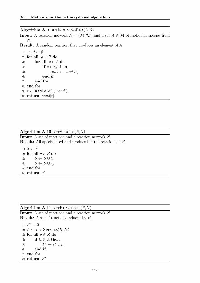
A.3. Methods for the pathway-based algorithms
Algorithm A.9 getIncomingRea(A,N)
Input: A reaction network N = (M,R), and a set A ∈ M of molecular species fromN .
Result: A random reaction that produces an element of A.
1: cand← ∅2: for all ρ ∈ R do3: for all s ∈ A do4: if s ∈ rρ then5: cand← cand ∪ ρ6: end if7: end for8: end for9: r ← random(1, |cand|)
10: return cand[r]
Algorithm A.10 getSpecies(R,N)
Input: A set of reactions and a reaction network N .Result: All species used and produced in the reactions in R.
1: S ← ∅2: for all ρ ∈ R do3: S ← S ∪ lρ4: S ← S ∪ rρ5: end for6: return S
Algorithm A.11 getReactions(R,N)
Input: A set of reactions and a reaction network N .Result: A set of reactions induced by R.
1: R′ ← ∅2: A← getSpecies(R,N)3: for all ρ ∈ R do4: if lρ ∈ A then5: R′ ← R′ ∪ ρ6: end if7: end for8: return R′
114
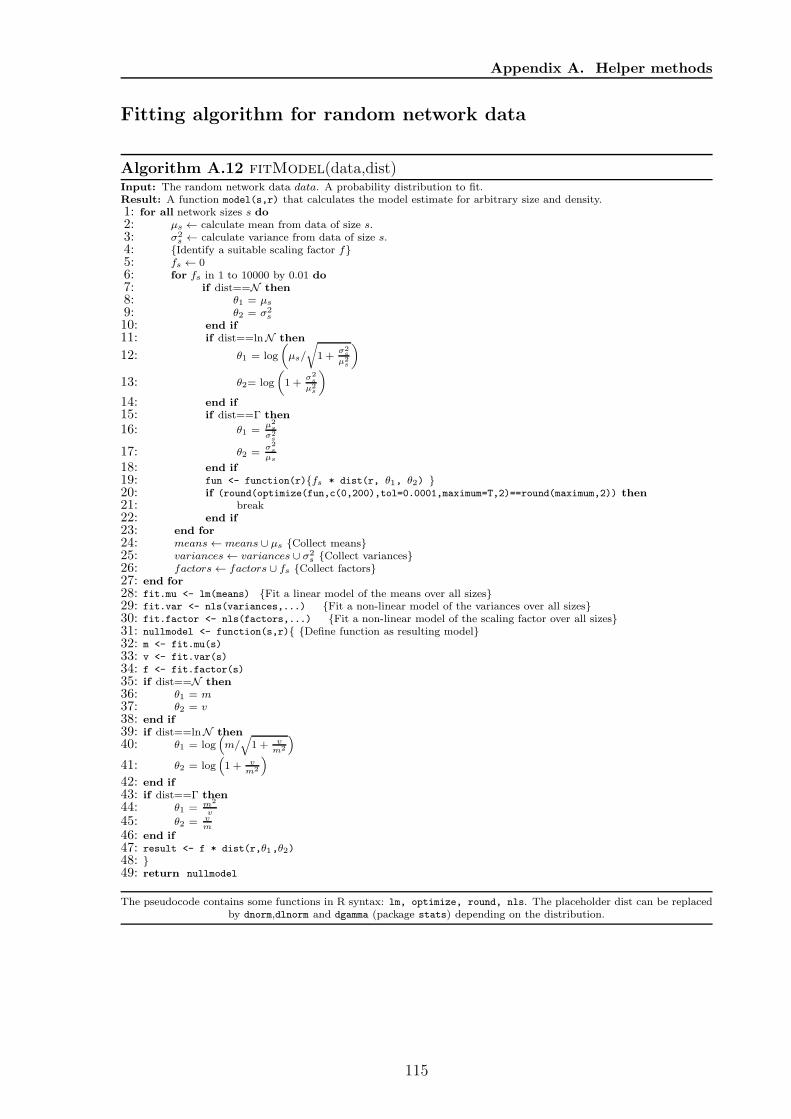
Appendix A. Helper methods
Fitting algorithm for random network data
Algorithm A.12 fitModel(data,dist)Input: The random network data data. A probability distribution to fit.Result: A function model(s,r) that calculates the model estimate for arbitrary size and density.1: for all network sizes s do
2: µs ← calculate mean from data of size s.3: σ2
s ← calculate variance from data of size s.4: {Identify a suitable scaling factor f}5: fs ← 06: for fs in 1 to 10000 by 0.01 do
7: if dist==N then
8: θ1 = µs
9: θ2 = σ2s
10: end if
11: if dist==lnN then
12: θ1 = log
(
µs/
√
1 +σ2s
µ2s
)
13: θ2= log
(
1 +σ2
s
µ2s
)
14: end if
15: if dist==Γ then
16: θ1 =µ2
s
σ2s
17: θ2 =σ2
s
µs
18: end if
19: fun <- function(r){fs * dist(r, θ1, θ2) }20: if (round(optimize(fun,c(0,200),tol=0.0001,maximum=T,2)==round(maximum,2)) then
21: break22: end if
23: end for
24: means← means ∪ µs {Collect means}25: variances← variances ∪ σ2
s {Collect variances}26: factors← factors ∪ fs {Collect factors}27: end for
28: fit.mu <- lm(means) {Fit a linear model of the means over all sizes}29: fit.var <- nls(variances,...) {Fit a non-linear model of the variances over all sizes}30: fit.factor <- nls(factors,...) {Fit a non-linear model of the scaling factor over all sizes}31: nullmodel <- function(s,r){ {Define function as resulting model}32: m <- fit.mu(s)
33: v <- fit.var(s)
34: f <- fit.factor(s)
35: if dist==N then
36: θ1 = m37: θ2 = v38: end if
39: if dist==lnN then
40: θ1 = log(
m/√
1 + vm2
)
41: θ2 = log(
1 + vm2
)
42: end if
43: if dist==Γ then
44: θ1 = m2
v
45: θ2 = vm
46: end if
47: result <- f * dist(r,θ1,θ2)48: }49: return nullmodel
The pseudocode contains some functions in R syntax: lm, optimize, round, nls. The placeholder dist can be replacedby dnorm,dlnorm and dgamma (package stats) depending on the distribution.
115

A.3. Methods for the pathway-based algorithms
116
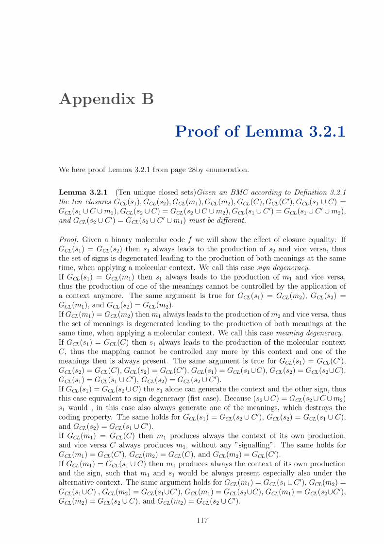
Appendix B
Proof of Lemma 3.2.1
We here proof Lemma 3.2.1 from page 28by enumeration.
Lemma 3.2.1 (Ten unique closed sets)Given an BMC according to Definition 3.2.1the ten closures GCL(s1), GCL(s2), GCL(m1), GCL(m2), GCL(C), GCL(C
′), GCL(s1 ∪ C) =GCL(s1 ∪C ∪m1), GCL(s2 ∪C) = GCL(s2 ∪C ∪m2), GCL(s1 ∪C ′) = GCL(s1 ∪C ′ ∪m2),and GCL(s2 ∪ C ′) = GCL(s2 ∪ C ′ ∪m1) must be different.
Proof. Given a binary molecular code f we will show the effect of closure equality: IfGCL(s1) = GCL(s2) then s1 always leads to the production of s2 and vice versa, thusthe set of signs is degenerated leading to the production of both meanings at the sametime, when applying a molecular context. We call this case sign degeneracy.If GCL(s1) = GCL(m1) then s1 always leads to the production of m1 and vice versa,thus the production of one of the meanings cannot be controlled by the application ofa context anymore. The same argument is true for GCL(s1) = GCL(m2), GCL(s2) =GCL(m1), and GCL(s2) = GCL(m2).If GCL(m1) = GCL(m2) thenm1 always leads to the production ofm2 and vice versa, thusthe set of meanings is degenerated leading to the production of both meanings at thesame time, when applying a molecular context. We call this case meaning degeneracy.If GCL(s1) = GCL(C) then s1 always leads to the production of the molecular contextC, thus the mapping cannot be controlled any more by this context and one of themeanings then is always present. The same argument is true for GCL(s1) = GCL(C
′),GCL(s2) = GCL(C), GCL(s2) = GCL(C
′), GCL(s1) = GCL(s1∪C), GCL(s2) = GCL(s2∪C),GCL(s1) = GCL(s1 ∪ C ′), GCL(s2) = GCL(s2 ∪ C ′).If GCL(s1) = GCL(s2∪C) the s1 alone can generate the context and the other sign, thusthis case equivalent to sign degeneracy (fist case). Because (s2∪C) = GCL(s2∪C ∪m2)s1 would , in this case also always generate one of the meanings, which destroys thecoding property. The same holds for GCL(s1) = GCL(s2 ∪ C ′), GCL(s2) = GCL(s1 ∪ C),and GCL(s2) = GCL(s1 ∪ C ′).If GCL(m1) = GCL(C) then m1 produces always the context of its own production,and vice versa C always produces m1, without any ”signalling”. The same holds forGCL(m1) = GCL(C
′), GCL(m2) = GCL(C), and GCL(m2) = GCL(C′).
If GCL(m1) = GCL(s1 ∪ C) then m1 produces always the context of its own productionand the sign, such that m1 and s1 would be always present especially also under thealternative context. The same argument holds for GCL(m1) = GCL(s1∪C ′), GCL(m2) =GCL(s1∪C) , GCL(m2) = GCL(s1∪C ′), GCL(m1) = GCL(s2∪C), GCL(m1) = GCL(s2∪C ′),GCL(m2) = GCL(s2 ∪ C), and GCL(m2) = GCL(s2 ∪ C ′).
117
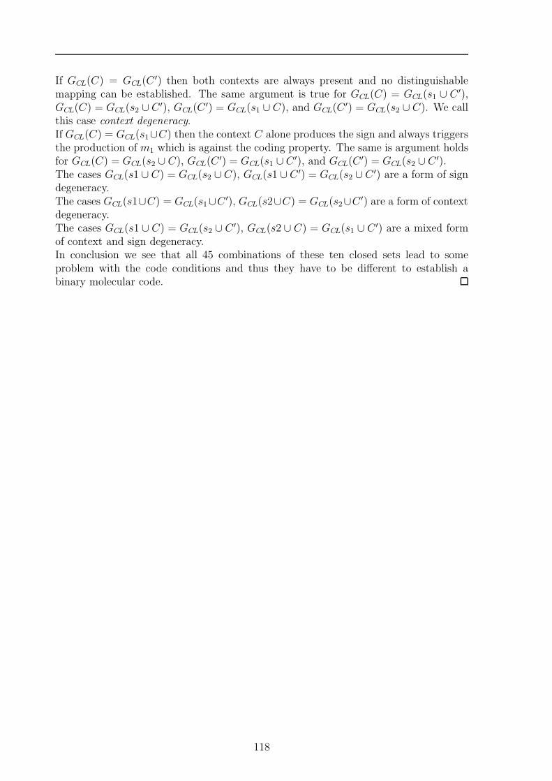
If GCL(C) = GCL(C′) then both contexts are always present and no distinguishable
mapping can be established. The same argument is true for GCL(C) = GCL(s1 ∪ C ′),GCL(C) = GCL(s2 ∪ C ′), GCL(C
′) = GCL(s1 ∪ C), and GCL(C′) = GCL(s2 ∪ C). We call
this case context degeneracy.If GCL(C) = GCL(s1∪C) then the context C alone produces the sign and always triggersthe production of m1 which is against the coding property. The same is argument holdsfor GCL(C) = GCL(s2 ∪ C), GCL(C
′) = GCL(s1 ∪ C ′), and GCL(C′) = GCL(s2 ∪ C ′).
The cases GCL(s1 ∪ C) = GCL(s2 ∪ C), GCL(s1 ∪ C ′) = GCL(s2 ∪ C ′) are a form of signdegeneracy.The cases GCL(s1∪C) = GCL(s1∪C ′), GCL(s2∪C) = GCL(s2∪C ′) are a form of contextdegeneracy.The cases GCL(s1 ∪ C) = GCL(s2 ∪ C ′), GCL(s2 ∪ C) = GCL(s1 ∪ C ′) are a mixed formof context and sign degeneracy.In conclusion we see that all 45 combinations of these ten closed sets lead to someproblem with the code conditions and thus they have to be different to establish abinary molecular code.
118
Appendix C
Potential codes in signaltransduction
119
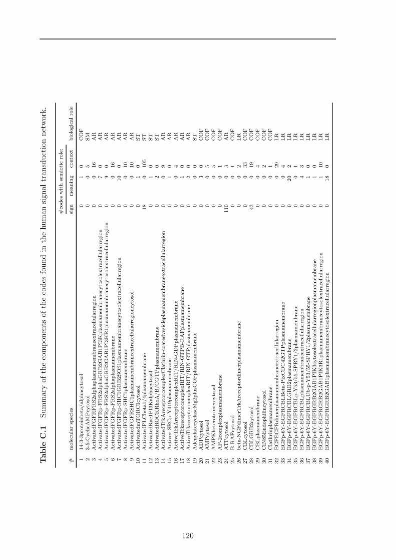
Table
C.1
Summaryof
thecompon
ents
ofthecodes
foundin
thehuman
sign
altran
sductionnetwork.
#co
des
withsemioticrole:
#molecu
larsp
ecies
sign
meaning
context
biologicalrole
114-3-3proteinbeta/alphacy
tosol
01
0COF
23-5-C
yclicAMPcy
tosol
00
5SM
3ActivatedFGFRFRS2alphaplasm
amem
braneextracellularregion
00
16
AR
4ActivatedFGFRp-F
RS2alphaGRB2GAB1PI3Kplasm
amem
branecytosolextracellularregion
07
0AR
5ActivatedFGFRp-F
RS2alphaGRB2GAB1PI3KR1plasm
amem
branecytosolextracellularregion
09
0AR
6ActivatedFGFRp-F
RS2alphaplasm
amem
brane
00
16
AR
7ActivatedFGFRp-SHC1GRB2SOS1plasm
amem
branecytosolextracellularregion
010
0AR
8ActivatedFGFRp-SHC1plasm
amem
brane
00
10
AR
9ActivatedFGFRSHC1plasm
amem
braneextracellularregioncy
tosol
00
10
AR
10
ActivatedmTORC1cy
tosol
01
0ST
11
ActivatedPLCbeta1/4plasm
amem
brane
18
0105
ST
12
ActivatedRac1PI3Kalphacy
tosol
01
0ST
13
ActivatedROCKRhoA/B/CGTPplasm
amem
brane
02
0ST
14
ActivatedTrkAreceptorcomplexClathrin-coatedvesicleplasm
amem
braneextracellularregion
00
9AR
15
Activec-SRCp-Y
419plasm
amem
brane
01
0AR
16
ActiveT
rkAreceptorcomplexRIT
/RIN
-GDPplasm
amem
brane
00
4AR
17
ActiveT
rkreceptorcomplexRIT
/RIN
-GTPB-R
AFplasm
amem
brane
01
0AR
18
ActiveT
rkreceptorcomplexRIT
/RIN
-GTPplasm
amem
brane
02
0AR
19
Aden
ylatecy
claseMg2plusC
OFplasm
amem
brane
00
0ST
20
ADPcy
tosol
03
0COF
21
AMPcy
tosol
00
5COF
22
AMPKheterotrim
ercy
tosol
00
5COF
23
AP-2complexplasm
amem
brane
00
1COF
24
ATPcy
tosol
110
03
AR
25
B-R
AFcy
tosol
00
1COF
26
beta-N
GFdim
erTrkAreceptord
imerplasm
amem
brane
00
2LR
27
CBLcy
tosol
00
33
COF
28
CBLGRB2cy
tosol
43
019
COF
29
CBLplasm
amem
brane
00
4COF
30
CIN
85Endophilincy
tosol
00
2COF
31
Clathrinplasm
amem
brane
00
1COF
32
EGFEGFRdim
erplasm
amem
braneextracellularregion
00
29
LR
33
EGFp-6Y-E
GFRCBLBeta-P
ixCDC42GTPplasm
amem
brane
00
4LR
34
EGFp-6Y-E
GFRCBLGRB2plasm
amem
brane
020
2LR
35
EGFp-6Y-E
GFRCBLp-Y
53/55-SPRY1/2plasm
amem
brane
00
1LR
36
EGFp-6Y-E
GFRCBLplasm
amem
braneextracellularregion
04
3LR
37
EGFp-6Y-E
GFRCBLUb-p-Y
53/55-SPRY1/2plasm
amem
brane
01
0LR
38
EGFp-6Y-E
GFRGRB2GAB1PIK
3cy
tosolextracellularregionplasm
amem
brane
01
0LR
39
EGFp-6Y-E
GFRGRB2GAB1PIK
3R1plasm
amem
branecytosolextracellularregion
01
10
LR
40
EGFp-6Y-E
GFRGRB2GAB1plasm
amem
branecytosolextracellularregion
018
0LR
120
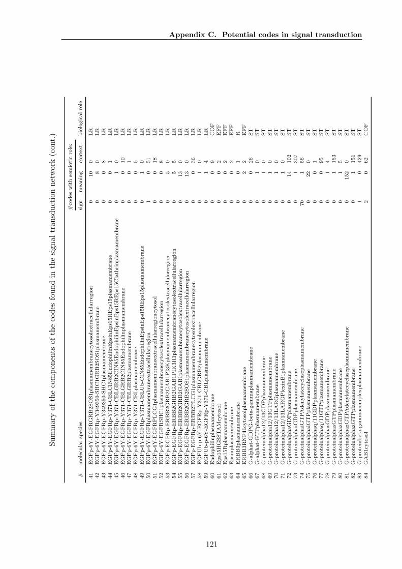
Appendix C. Potential codes in signal transduction
Summaryof
thecompon
ents
ofthecodes
foundin
thesign
altran
sductionnetwork(con
t.)
#co
des
withsemioticrole:
#molecu
larsp
ecies
sign
meaning
context
biologicalrole
41
EGFp-6Y-E
GFRGRB2SOS1plasm
amem
branecytosolextracellularregion
010
0LR
42
EGFp-6Y-E
GFRp-Y
349350-SHC1GRB2SOS1plasm
amem
brane
08
0LR
43
EGFp-6Y-E
GFRp-Y
349350-SHC1plasm
amem
brane
00
8LR
44
EGFp-6Y-E
GFRp-Y
371-C
BLCIN
85EndophilinEpsinEps15REps15plasm
amem
brane
00
1LR
45
EGFp-6Y-E
GFRp-Y
371-C
BLGRB2CIN
85EndophilinEpsinEps15REps15Clathrinplasm
amem
brane
01
0LR
46
EGFp-6Y-E
GFRp-Y
371-C
BLGRB2CIN
85Endophilinplasm
amem
brane
00
10
LR
47
EGFp-6Y-E
GFRp-Y
371-C
BLGRB2plasm
amem
brane
00
1LR
48
EGFp-6Y-E
GFRp-Y
371-C
BLplasm
amem
brane
00
5LR
49
EGFp-6Y-E
GFRp-Y
371-C
BLUb-C
IN85EndophilinEpsinEps15REps15plasm
amem
brane
01
0LR
50
EGFp-6Y-E
GFRplasm
amem
braneextracellularregion
10
51
LR
51
EGFp-6Y-E
GFRPLCG1plasm
amem
braneextracellularregioncy
tosol
00
18
LR
52
EGFp-6Y-E
GFRSHC1plasm
amem
branecytosolextracellularregion
00
8LR
53
EGFp-E
GFRp-E
RBB2GRB2GAB1PI3Kplasm
amem
branecytosolextracellularregion
05
0LR
54
EGFp-E
GFRp-E
RBB2GRB2GAB1PIK
3R1plasm
amem
branecytosolextracellularregion
05
5LR
55
EGFp-E
GFRp-E
RBB2GRB2GAB1plasm
amem
branecytosolextracellularregion
013
0LR
56
EGFp-E
GFRp-E
RBB2GRB2SOS1plasm
amem
branecytosolextracellularregion
013
0LR
57
EGFp-E
GFRp-E
RBB2PLCG1plasm
amem
branecytosolextracellularregion
00
36
LR
58
EGFUb-p-6Y-E
GFRp-Y
371-C
BLGRB2plasm
amem
brane
01
0LR
59
EGFUb-p-6Y-E
GFRp-Y
371-C
BLplasm
amem
brane
01
4LR
60
Endophilinplasm
amem
brane
00
9COF
61
Eps15HGSSTAMcy
tosol
00
2EFF
62
Eps15Rplasm
amem
brane
00
2EFF
63
Epsinplasm
amem
brane
00
2EFF
64
ERBB3plasm
amem
brane
00
1R
65
ERBB3RNF41cy
tosolplasm
amem
brane
02
2EFF
66
G-alphat-GDPG-beta-gammaplasm
amem
brane
00
26
ST
67
G-alphat-GTPplasm
amem
brane
01
0ST
68
G-proteinalpha12/13GDPplasm
amem
brane
01
0ST
69
G-proteinalpha12/13GTPplasm
amem
brane
01
0ST
70
G-proteinalpha12/13LARGplasm
amem
brane
01
0ST
71
G-proteinalpha12/13LARGPlexinB1plasm
amem
brane
01
0ST
72
G-proteinalphaGDPplasm
amem
brane
014
102
ST
73
G-proteinalphaiG
DPplasm
amem
brane
01
307
ST
74
G-proteinalphaiG
TPAden
ylatecy
claseplasm
amem
brane
70
156
ST
75
G-proteinalphaiG
TPplasm
amem
brane
022
0ST
76
G-proteinalphaq/11GDPplasm
amem
brane
00
1ST
77
G-proteinalphaq/11GTPplasm
amem
brane
00
95
ST
78
G-proteinalphasG
DPplasm
amem
brane
01
4ST
79
G-proteinalphasG
TPplasm
amem
brane
01
153
ST
80
G-proteinalphazG
DPplasm
amem
brane
01
5ST
81
G-proteinalphazG
TPAden
ylatecy
claseplasm
amem
brane
0152
0ST
82
G-proteinalphazG
TPplasm
amem
brane
01
151
ST
83
G-proteinbeta-gammacomplexplasm
amem
brane
10
429
ST
84
GAB1cy
tosol
20
62
COF
121
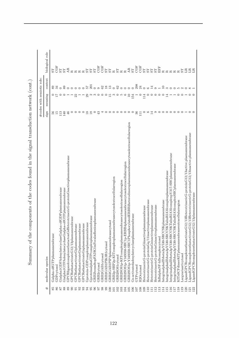
Summaryof
thecompon
ents
ofthecodes
foundin
thesign
altran
sductionnetwork(con
t.)
#co
des
withsemioticrole:
#molecu
larsp
ecies
sign
meaning
context
biologicalrole
85
Galpha-olfGTPplasm
amem
brane
56
089
ST
86
GDPcy
tosol
15
17
34
COF
87
Gialpha1GDPAden
ylatecy
claseGalpha-olfGDPplasm
amem
brane
113
00
ST
88
Gialpha1GTPAden
ylatecy
claseGalpha-olfGTPplasm
amem
brane
140
089
ST
89
GPCRligandcomplexesthatactonGsH
eterotrim
ericG-proteinGsactivep
lasm
amem
brane
46
10
AR
90
GPCRsthatactivateG12/13plasm
amem
brane
01
0R
91
GPCRsthatactivateGiplasm
amem
brane
022
0R
92
GPCRsthatactivateGsp
lasm
amem
brane
01
0R
93
GPCRsthatactivateGzp
lasm
amem
brane
01
0R
94
Gprotein-G
DPcomplexplasm
amem
brane
18
29
57
ST
95
GproteinalphaGTPcomplexplasm
amem
brane
18
2201
ST
96
GRB2boundtopFADK1inFocaladhesionplasm
amem
brane
03
0ST
97
GRB2cy
tosol
43
09
COF
98
GRB2GAB1cy
tosol
40
62
COF
99
GRB2GAB1PIK
3R1cy
tosol
00
18
ST
100
GRB2GAB1PIP
3plasm
amem
branecytosol
015
13
ST
101
GRB2p-SHP2p-K
ITcomplexplasm
amem
branecytosolextracellularregion
03
0R
102
GRB2SOS1cy
tosol
00
62
ST
103
GRB2SOS1p-K
ITcomplexplasm
amem
branecytosolextracellularregion
05
0R
104
GRB2SOS1p-Y
349350-SHC1p-E
RBB4plasm
amem
branecytosolextracellularregion
06
0R
105
GRB2SOS1p-Y
349350-SHC1Phosp
horylatedERBB2heterodim
ersp
lasm
amem
branecytosolextracellularregion
010
0AR
106
Gs-activatedaden
ylatecy
claseplasm
amem
brane
0154
0ST
107
GTPcy
tosol
36
1298
COF
108
H2Ocy
tosol
111
024
COF
109
Heterotrim
ericG-proteinGiinactivep
lasm
amem
brane
0114
0ST
110
Heterotrim
ericG-proteinGq/11inactivep
lasm
amem
brane
60
6ST
111
Heterotrim
ericG-proteinGsinactivep
lasm
amem
brane
14
014
ST
112
Heterotrim
ericG-proteinGzinactivep
lasm
amem
brane
90
9ST
113
IkBalphaNF-kBcomplexcy
tosol
00
1EFF
114
IntegrinalphaIIbbeta3pY530-SRCCSKplasm
amem
brane
00
10
R115
IntegrinalphaIIbbeta3pY530-SRCCSKTalinRIA
Mcomplexplasm
amem
brane
014
3R
116
IntegrinalphaIIbbeta3pY530-SRCCSKTalinRIA
McomplexpY317-SHCplasm
amem
brane
01
0R
117
IntegrinalphaIIbbeta3pY530-SRCCSKTalinRIA
McomplexSHCplasm
amem
brane
01
0R
118
KIT
sSCFdim
erKIT
plasm
amem
braneextracellularregion
00
5R
119
Largva
riant1cy
tosol
00
2ST
120
LigandGPCRcomplexesthatactivateG12/13Heterotrim
ericG-proteinG12/13active.plasm
amem
brane
11
0LR
121
LigandGPCRcomplexesthatactivateG12/13Heterotrim
ericG-proteinG12/13inactive.plasm
amem
brane
00
8LR
122
LigandGPCRcomplexesthatactivateG12/13plasm
amem
brane
00
1LR
122
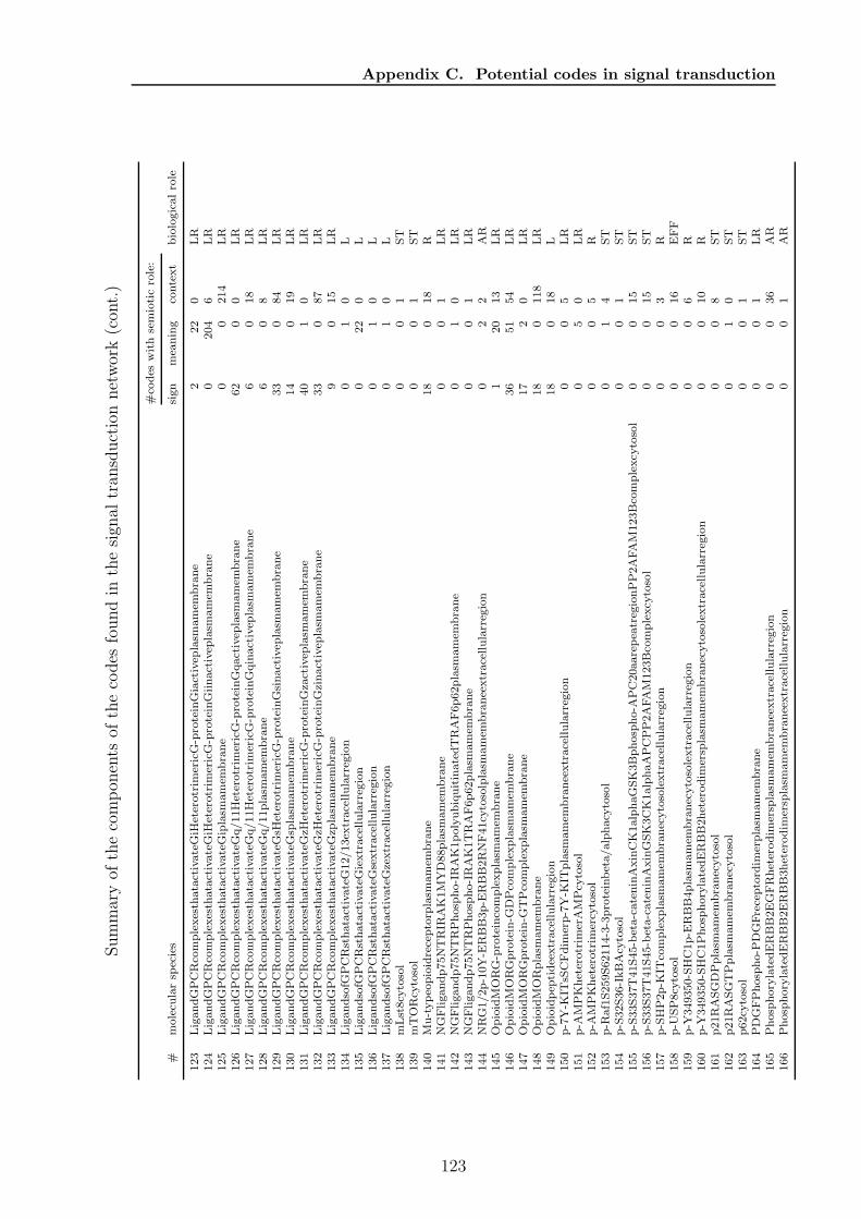
Appendix C. Potential codes in signal transduction
Summaryof
thecompon
ents
ofthecodes
foundin
thesign
altran
sductionnetwork(con
t.)
#co
des
withsemioticrole:
#molecu
larsp
ecies
sign
meaning
context
biologicalrole
123
LigandGPCRcomplexesthatactivateGiH
eterotrim
ericG-proteinGiactivep
lasm
amem
brane
222
0LR
124
LigandGPCRcomplexesthatactivateGiH
eterotrim
ericG-proteinGiinactivep
lasm
amem
brane
0204
6LR
125
LigandGPCRcomplexesthatactivateGiplasm
amem
brane
00
214
LR
126
LigandGPCRcomplexesthatactivateGq/11Heterotrim
ericG-proteinGqactivep
lasm
amem
brane
62
00
LR
127
LigandGPCRcomplexesthatactivateGq/11Heterotrim
ericG-proteinGqinactivep
lasm
amem
brane
60
18
LR
128
LigandGPCRcomplexesthatactivateGq/11plasm
amem
brane
60
8LR
129
LigandGPCRcomplexesthatactivateGsH
eterotrim
ericG-proteinGsinactivep
lasm
amem
brane
33
084
LR
130
LigandGPCRcomplexesthatactivateGsp
lasm
amem
brane
14
019
LR
131
LigandGPCRcomplexesthatactivateGzH
eterotrim
ericG-proteinGzactivep
lasm
amem
brane
40
10
LR
132
LigandGPCRcomplexesthatactivateGzH
eterotrim
ericG-proteinGzinactivep
lasm
amem
brane
33
087
LR
133
LigandGPCRcomplexesthatactivateGzp
lasm
amem
brane
90
15
LR
134
LigandsofG
PCRsthatactivateG12/13ex
tracellularregion
01
0L
135
LigandsofG
PCRsthatactivateGiextracellularregion
022
0L
136
LigandsofG
PCRsthatactivateGsextracellularregion
01
0L
137
LigandsofG
PCRsthatactivateGzextracellularregion
01
0L
138
mLst8cy
tosol
00
1ST
139
mTORcy
tosol
00
1ST
140
Mu-typeopioidreceptorp
lasm
amem
brane
18
018
R141
NGFligandp75NTRIR
AK1MYD88plasm
amem
brane
00
1LR
142
NGFligandp75NTRPhosp
ho-IRAK1polyubiquitinatedTRAF6p62plasm
amem
brane
01
0LR
143
NGFligandp75NTRPhosp
ho-IRAK1TRAF6p62plasm
amem
brane
00
1LR
144
NRG1/2p-10Y-E
RBB3p-E
RBB2RNF41cy
tosolplasm
amem
braneextracellularregion
02
2AR
145
OpioidMORG-proteincomplexplasm
amem
brane
120
13
LR
146
OpioidMORGprotein-G
DPcomplexplasm
amem
brane
36
51
54
LR
147
OpioidMORGprotein-G
TPcomplexplasm
amem
brane
17
20
LR
148
OpioidMORplasm
amem
brane
18
0118
LR
149
Opioidpep
tideextracellularregion
18
018
L150
p-7Y-K
ITsS
CFdim
erp-7Y-K
ITplasm
amem
braneextracellularregion
00
5LR
151
p-A
MPKheterotrim
erAMPcy
tosol
05
0LR
152
p-A
MPKheterotrim
ercy
tosol
00
5R
153
p-R
af1S259S62114-3-3proteinbeta/alphacy
tosol
01
4ST
154
p-S32S36-IkBAcy
tosol
00
1ST
155
p-S33S37T41S45-beta-cateninAxinCK1alphaGSK3Bphosp
ho-A
PC20aarepeatregionPP2AFAM123Bcomplexcy
tosol
00
15
ST
156
p-S33S37T41S45-beta-cateninAxinGSK3CK1alphaAPCPP2AFAM123Bco
mplexcy
tosol
00
15
ST
157
p-SHP2p-K
ITcomplexplasm
amem
branecytosolextracellularregion
00
3R
158
p-U
SP8cy
tosol
00
16
EFF
159
p-Y
349350-SHC1p-E
RBB4plasm
amem
branecytosolextracellularregion
00
6R
160
p-Y
349350-SHC1Phosp
horylatedERBB2heterodim
ersp
lasm
amem
branecytosolextracellularregion
00
10
R161
p21RASGDPplasm
amem
branecytosol
00
8ST
162
p21RASGTPplasm
amem
branecytosol
01
0ST
163
p62cy
tosol
00
1ST
164
PDGFPhosp
ho-P
DGFreceptord
imerplasm
amem
brane
00
1LR
165
Phosp
horylatedERBB2EGFRheterodim
ersp
lasm
amem
braneextracellularregion
00
36
AR
166
Phosp
horylatedERBB2ERBB3heterodim
ersp
lasm
amem
braneextracellularregion
00
1AR
123
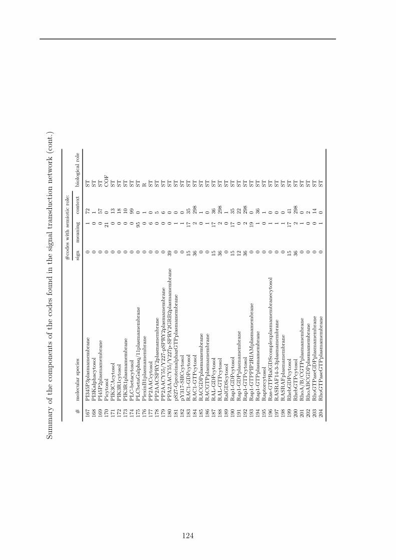
Summaryof
thecompon
ents
ofthecodes
foundin
thesign
altran
sductionnetwork(con
t.)
#co
des
withsemioticrole:
#molecu
larsp
ecies
sign
meaning
context
biologicalrole
167
PI345P3plasm
amem
brane
01
72
ST
168
PI3Kalphacy
tosol
00
1ST
169
PI45P2plasm
amem
brane
00
57
ST
170
Picytosol
021
0COF
171
PIK
3CAcy
tosol
00
13
ST
172
PIK
3R1cy
tosol
00
18
ST
173
PIK
3R1plasm
amem
brane
00
10
ST
174
PLC-betacy
tosol
00
99
ST
175
PLCbetaGalphaq/11plasm
amem
brane
095
0ST
176
PlexinB1plasm
amem
brane
00
1R
177
PP2AACcy
tosol
06
0ST
178
PP2AACSPRY2plasm
amem
brane
00
5ST
179
PP2AACY55/Y227-pSPRY2plasm
amem
brane
00
6ST
180
PPA2AACY55/Y227p-SPRY2GRB2plasm
amem
brane
39
00
ST
181
pS27-G
proteinalphazG
TPplasm
amem
brane
01
0ST
182
pY317-SHCcy
tosol
01
0ST
183
RAC1-G
DPcy
tosol
15
17
35
ST
184
RAC1-G
TPcy
tosol
36
2298
ST
185
RACGDPplasm
amem
brane
00
1ST
186
RACGTPplasm
amem
brane
01
0ST
187
RAL-G
DPcy
tosol
15
17
36
ST
188
RAL-G
TPcy
tosol
36
2298
ST
189
RalG
DScy
tosol
00
1ST
190
Rap1-G
DPcy
tosol
15
17
35
ST
191
Rap1-G
DPplasm
amem
brane
12
022
ST
192
Rap1-G
TPcy
tosol
36
2298
ST
193
Rap1-G
TPPIP
2RIA
Mplasm
amem
brane
019
0ST
194
Rap1-G
TPplasm
amem
brane
01
36
ST
195
Raptorcytosol
00
1ST
196
Ras-GTPRalG
DScomplexplasm
amem
branecytosol
01
0ST
197
RASRAF14-3-3plasm
amem
brane
01
0ST
198
RASRAFplasm
amem
brane
01
0ST
199
Rheb
GDPcy
tosol
15
17
41
ST
200
Rheb
GTPcy
tosol
36
2298
ST
201
RhoA/B/CGTPplasm
amem
brane
01
0ST
202
RhoABCGDPplasm
amem
brane
00
2ST
203
RhoGTPaseGDPplasm
amem
brane
00
14
ST
204
RhoGTPaseGTPplasm
amem
brane
01
0ST
124
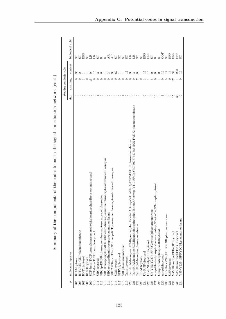
Appendix C. Potential codes in signal transduction
Summaryof
thecompon
ents
ofthecodes
foundin
thesign
altran
sductionnetwork(con
t.)
#co
des
semioticrole
#molecu
larsp
ecies
sign
meaning
context
biologicalrole
205
RIA
Mcy
tosol
00
36
ST
206
RIT
/RIN
-GDPplasm
amem
brane
00
2ST
207
RNF41cy
tosol
01
1EFF
208
ROCKcy
tosol
00
1ST
209
SCF-beta-T
rCP1complexassociatedwithphosp
horylatedbeta-catenincy
tosol
015
0LR
210
SCF-beta-T
rCP1complexcy
tosol
00
15
LR
211
SHC1cy
tosol
10
3ST
212
SHC1p-E
RBB4plasm
amem
branecytosolextracellularregion
00
6R
213
SHC1Phosp
horylatedERBB2heterodim
ersp
lasm
amem
branecytosolextracellularregion
00
10
R214
SHCactivatedinsu
linreceptorp
lasm
amem
brane
00
3AR
215
SHP2SFKsp
-KIT
sSCFdim
erp-K
ITplasm
amem
branecytosolextracellularregion
00
3AR
216
SOS1cy
tosol
00
62
ST
217
SPRY1/2cy
tosol
00
1ST
218
SRCplasm
amem
brane
10
1ST
219
Talin-1cy
tosol
00
17
ST
220
TalinRIA
McomplexECMligandsalphaIIbbeta3Activep
-Y419-SRCpY397-FADK1plasm
amem
brane
00
3LR
221
TalinRIA
McomplexECMligandsIntegrinalphaIIbbeta3Activep
-Y419-SRCpY397407576577861925-FADK1plasm
amem
brane
00
3LR
222
TalinRIA
Mcomplexplasm
amem
brane
07
0ST
223
TRAF6cy
tosol
00
1ST
224
Ub-R
NF41cy
tosol
01
15
EFF
225
Ub-R
NF41p-U
SP8cy
tosol
01
15
EFF
226
Ub-Y
55/Y227p-SPRY2cy
tosolplasm
amem
brane
05
0ST
227
ubiquitinatedphosp
ho-beta-cateninSCFbeta-T
rCP1complexcy
tosol
16
00
R228
Ubiquitinatedphosp
ho-IkBcy
tosol
01
0R
229
ubiquitincy
tosol
10
16
COF
230
UbY55/Y227-pSPRY2CBLplasm
amem
brane
05
14
ST
231
USP8cy
tosol
00
16
EFF
232
VAV1Rho/RacE
FFsG
DPcy
tosol
15
17
34
EFF
233
VAV1Rho/RacE
FFsG
TPcy
tosol
36
1298
EFF
234
Y55/Y227-pSPRY2CBLplasm
amem
brane
00
19
ST
125

126
Appendix D
Potential codes in metabolism
127
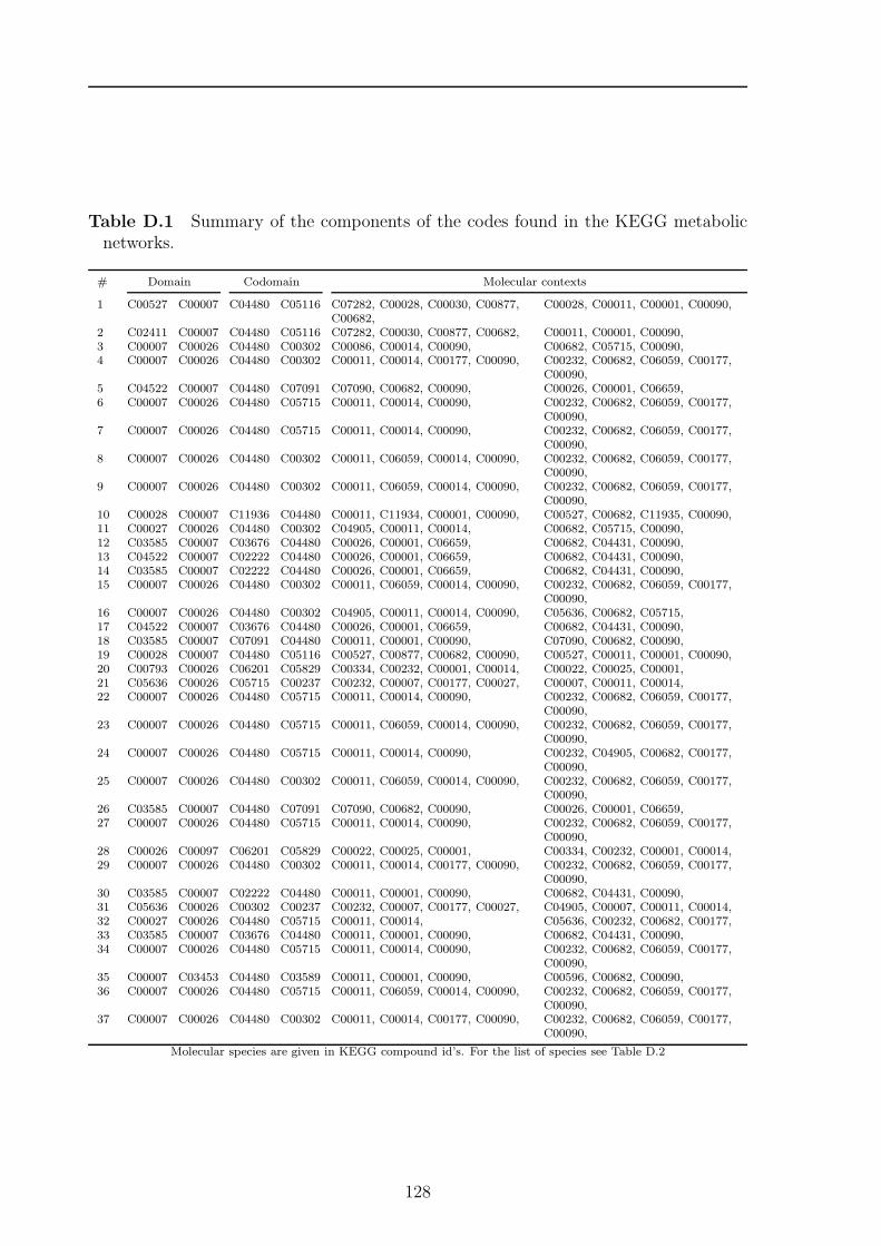
Table D.1 Summary of the components of the codes found in the KEGG metabolicnetworks.
# Domain Codomain Molecular contexts
1 C00527 C00007 C04480 C05116 C07282, C00028, C00030, C00877,C00682,
C00028, C00011, C00001, C00090,
2 C02411 C00007 C04480 C05116 C07282, C00030, C00877, C00682, C00011, C00001, C00090,3 C00007 C00026 C04480 C00302 C00086, C00014, C00090, C00682, C05715, C00090,4 C00007 C00026 C04480 C00302 C00011, C00014, C00177, C00090, C00232, C00682, C06059, C00177,
C00090,5 C04522 C00007 C04480 C07091 C07090, C00682, C00090, C00026, C00001, C06659,6 C00007 C00026 C04480 C05715 C00011, C00014, C00090, C00232, C00682, C06059, C00177,
C00090,7 C00007 C00026 C04480 C05715 C00011, C00014, C00090, C00232, C00682, C06059, C00177,
C00090,8 C00007 C00026 C04480 C00302 C00011, C06059, C00014, C00090, C00232, C00682, C06059, C00177,
C00090,9 C00007 C00026 C04480 C00302 C00011, C06059, C00014, C00090, C00232, C00682, C06059, C00177,
C00090,10 C00028 C00007 C11936 C04480 C00011, C11934, C00001, C00090, C00527, C00682, C11935, C00090,11 C00027 C00026 C04480 C00302 C04905, C00011, C00014, C00682, C05715, C00090,12 C03585 C00007 C03676 C04480 C00026, C00001, C06659, C00682, C04431, C00090,13 C04522 C00007 C02222 C04480 C00026, C00001, C06659, C00682, C04431, C00090,14 C03585 C00007 C02222 C04480 C00026, C00001, C06659, C00682, C04431, C00090,15 C00007 C00026 C04480 C00302 C00011, C06059, C00014, C00090, C00232, C00682, C06059, C00177,
C00090,16 C00007 C00026 C04480 C00302 C04905, C00011, C00014, C00090, C05636, C00682, C05715,17 C04522 C00007 C03676 C04480 C00026, C00001, C06659, C00682, C04431, C00090,18 C03585 C00007 C07091 C04480 C00011, C00001, C00090, C07090, C00682, C00090,19 C00028 C00007 C04480 C05116 C00527, C00877, C00682, C00090, C00527, C00011, C00001, C00090,20 C00793 C00026 C06201 C05829 C00334, C00232, C00001, C00014, C00022, C00025, C00001,21 C05636 C00026 C05715 C00237 C00232, C00007, C00177, C00027, C00007, C00011, C00014,22 C00007 C00026 C04480 C05715 C00011, C00014, C00090, C00232, C00682, C06059, C00177,
C00090,23 C00007 C00026 C04480 C05715 C00011, C06059, C00014, C00090, C00232, C00682, C06059, C00177,
C00090,24 C00007 C00026 C04480 C05715 C00011, C00014, C00090, C00232, C04905, C00682, C00177,
C00090,25 C00007 C00026 C04480 C00302 C00011, C06059, C00014, C00090, C00232, C00682, C06059, C00177,
C00090,26 C03585 C00007 C04480 C07091 C07090, C00682, C00090, C00026, C00001, C06659,27 C00007 C00026 C04480 C05715 C00011, C00014, C00090, C00232, C00682, C06059, C00177,
C00090,28 C00026 C00097 C06201 C05829 C00022, C00025, C00001, C00334, C00232, C00001, C00014,29 C00007 C00026 C04480 C00302 C00011, C00014, C00177, C00090, C00232, C00682, C06059, C00177,
C00090,30 C03585 C00007 C02222 C04480 C00011, C00001, C00090, C00682, C04431, C00090,31 C05636 C00026 C00302 C00237 C00232, C00007, C00177, C00027, C04905, C00007, C00011, C00014,32 C00027 C00026 C04480 C05715 C00011, C00014, C05636, C00232, C00682, C00177,33 C03585 C00007 C03676 C04480 C00011, C00001, C00090, C00682, C04431, C00090,34 C00007 C00026 C04480 C05715 C00011, C00014, C00090, C00232, C00682, C06059, C00177,
C00090,35 C00007 C03453 C04480 C03589 C00011, C00001, C00090, C00596, C00682, C00090,36 C00007 C00026 C04480 C05715 C00011, C06059, C00014, C00090, C00232, C00682, C06059, C00177,
C00090,37 C00007 C00026 C04480 C00302 C00011, C00014, C00177, C00090, C00232, C00682, C06059, C00177,
C00090,
Molecular species are given in KEGG compound id’s. For the list of species see Table D.2
128
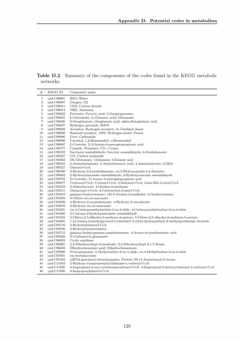
Appendix D. Potential codes in metabolism
Table D.2 Summary of the components of the codes found in the KEGG metabolicnetworks.
# KEGG ID Compound name
1 cpd:C00001 H2O; Water2 cpd:C00007 Oxygen; O23 cpd:C00011 CO2; Carbon dioxide4 cpd:C00014 NH3; Ammonia5 cpd:C00022 Pyruvate; Pyruvic acid; 2-Oxopropanoate;6 cpd:C00025 L-Glutamate; L-Glutamic acid; Glutamate7 cpd:C00026 2-Oxoglutarate; Oxoglutaric acid; alpha-Ketoglutaric acid8 cpd:C00027 Hydrogen peroxide; H2O29 cpd:C00028 Acceptor; Hydrogen-acceptor; A; Oxidized donor
10 cpd:C00030 Reduced acceptor; AH2; Hydrogen-donor; Donor11 cpd:C00086 Urea; Carbamide12 cpd:C00090 Catechol; 1,2-Benzenediol; o-Benzenediol13 cpd:C00097 L-Cysteine; L-2-Amino-3-mercaptopropionic acid14 cpd:C00177 Cyanide; Prussiate; CN-; Cyano15 cpd:C00232 Succinate semialdehyde; Succinic semialdehyde; 4-Oxobutanoate16 cpd:C00237 CO; Carbon monoxide17 cpd:C00302 DL-Glutamate; Glutamate; Glutamic acid18 cpd:C00334 4-Aminobutanoate; 4-Aminobutanoic acid; 4-Aminobutyrate; GABA19 cpd:C00527 Glutaryl-CoA20 cpd:C00596 2-Hydroxy-2,4-pentadienoate; cis-2-Hydroxypenta-2,4-dienoate;21 cpd:C00682 2-Hydroxymuconate semialdehyde; 2-Hydroxymuconic semialdehyde22 cpd:C00793 D-Cysteine; D-Amino-3-mercaptopropionic acid23 cpd:C00877 Crotonoyl-CoA; Crotonyl-CoA; 2-Butenoyl-CoA; trans-But-2-enoyl-CoA24 cpd:C02222 2-Maleylacetate; 4-Oxohex-2-enedioate25 cpd:C02411 Glutaconyl-1-CoA; 4-Carboxybut-2-enoyl-CoA26 cpd:C03453 gamma-Oxalocrotonate; (Z)-5-Oxohex-2-enedioate; 4-Oxalocrotonate27 cpd:C03585 3-Chloro-cis,cis-muconate28 cpd:C03589 4-Hydroxy-2-oxopentanoate; 4-Hydroxy-2-oxovalerate29 cpd:C03676 3-Hydroxy-cis,cis-muconate30 cpd:C04431 cis-4-Carboxymethylenebut-2-en-4-olide; 4-Carboxymethylenebut-2-en-4-olide31 cpd:C04480 3-Carboxy-2-hydroxymuconate semialdehyde32 cpd:C04522 2-Chloro-2,5-dihydro-5-oxofuran-2-acetate; 5-Chloro-2,5-dihydro-2-oxofuran-5-acetate33 cpd:C04905 1-(4-Amino-2-methylpyrimid-5-ylmethyl)-3-(beta-hydroxyethyl)-2-methylpyridinium bromide34 cpd:C05116 3-Hydroxybutanoyl-CoA35 cpd:C05636 3-Hydroxykynurenamine36 cpd:C05715 gamma-Amino-gamma-cyanobutanoate; 4-Amino-4-cyanobutanoic acid37 cpd:C05829 N-Carbamyl-L-glutamate38 cpd:C06059 Cyclic amidines39 cpd:C06201 2,4-Dihydroxyhept-2-enedioate; 2,4-Dihydroxyhept-2-1,7-dioate40 cpd:C06659 Dihydroclavaminic acid; Dihydroclavaminate41 cpd:C07090 Protoanemonin; 4-Methylenebut-2-en-4-olide; cis-4-Methylenebut-2-en-4-olide42 cpd:C07091 cis-Acetylacrylate43 cpd:C07282 [eIF5A-precursor]-deoxyhypusine; Protein N6-(4-Aminobutyl)-L-lysine44 cpd:C11934 2-Hydroxy-4-isopropenylcyclohexane-1-carboxyl-CoA45 cpd:C11935 4-Isopropenyl-2-oxy-cyclohexanecarboxyl-CoA; 4-Isopropenyl-2-ketocyclohexane-1-carboxyl-CoA46 cpd:C11936 3-Isopropenylpimelyl-CoA
129

130
Appendix E
Networks
The network models are all in REA-format. The REA-format is a plain text format forchemical reaction networks and basically contains the number of molecular species, a listof molecular species, the number of reactions and the list of reactions. Stoichiometricinformation is maintained, while kinetics are not represented in .rea-files.All networks are provided on the supplementary CD.
131
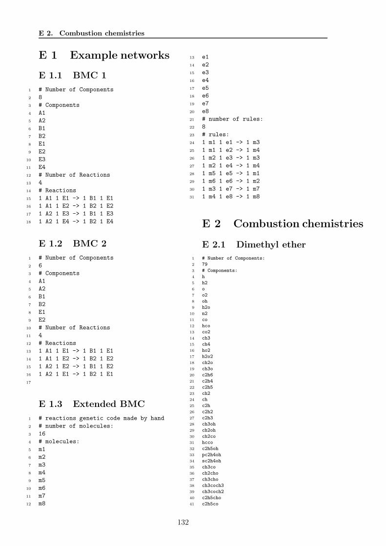
E 2. Combustion chemistries
E 1 Example networks
E 1.1 BMC 1
1 # Number of Components
2 8
3 # Components
4 A1
5 A2
6 B1
7 B2
8 E1
9 E2
10 E3
11 E4
12 # Number of Reactions
13 4
14 # Reactions
15 1 A1 1 E1 -> 1 B1 1 E1
16 1 A1 1 E2 -> 1 B2 1 E2
17 1 A2 1 E3 -> 1 B1 1 E3
18 1 A2 1 E4 -> 1 B2 1 E4
E 1.2 BMC 2
1 # Number of Components
2 6
3 # Components
4 A1
5 A2
6 B1
7 B2
8 E1
9 E2
10 # Number of Reactions
11 4
12 # Reactions
13 1 A1 1 E1 -> 1 B1 1 E1
14 1 A1 1 E2 -> 1 B2 1 E2
15 1 A2 1 E2 -> 1 B1 1 E2
16 1 A2 1 E1 -> 1 B2 1 E1
17
E 1.3 Extended BMC
1 # reactions genetic code made by hand
2 # number of molecules:
3 16
4 # molecules:
5 m1
6 m2
7 m3
8 m4
9 m5
10 m6
11 m7
12 m8
13 e1
14 e2
15 e3
16 e4
17 e5
18 e6
19 e7
20 e8
21 # number of rules:
22 8
23 # rules:
24 1 m1 1 e1 -> 1 m3
25 1 m1 1 e2 -> 1 m4
26 1 m2 1 e3 -> 1 m3
27 1 m2 1 e4 -> 1 m4
28 1 m5 1 e5 -> 1 m1
29 1 m6 1 e6 -> 1 m2
30 1 m3 1 e7 -> 1 m7
31 1 m4 1 e8 -> 1 m8
E 2 Combustion chemistries
E 2.1 Dimethyl ether
1 # Number of Components:
2 79
3 # Components:
4 h
5 h2
6 o
7 o2
8 oh
9 h2o
10 n2
11 co
12 hco
13 co2
14 ch3
15 ch4
16 ho2
17 h2o2
18 ch2o
19 ch3o
20 c2h6
21 c2h4
22 c2h5
23 ch2
24 ch
25 c2h
26 c2h2
27 c2h3
28 ch3oh
29 ch2oh
30 ch2co
31 hcco
32 c2h5oh
33 pc2h4oh
34 sc2h4oh
35 ch3co
36 ch2cho
37 ch3cho
38 ch3coch3
39 ch3coch2
40 c2h5cho
41 c2h5co
132
Appendix E. Networks
42 c2h5o
43 ch3o2
44 c2h5o2
45 ch3o2h
46 c2h5o2h
47 c2h3o1-2
48 ch3co2
49 c2h4o1-2
50 c2h4o2h
51 o2c2h4oh
52 ch3co3
53 ch3co3h
54 c2h3co
55 c2h3cho
56 ch3coch2o2
57 ch3coch2o2h
58 ch3coch2o
59 hco3h
60 hco3
61 hco2
62 o2c2h4o2h
63 ch2(s)
64 ch3och3
65 ch3och2
66 ch3och2o2
67 ch2och2o2h
68 ch3och2o2h
69 ch3och2o
70 o2ch2och2o2h
71 ho2ch2ocho
72 och2ocho
73 hoch2oco
74 hoch2o
75 hco2h
76 ch3ocho
77 ch3oco
78 ch2ocho
79 ch3och2oh
80 hoch2o2h
81 och2o2h
82 hoch2o2
83 # Number of Reactions:
84 708
85 # Reactions:
86 1 ch3 1 h -> 1 ch4
87 1 ch4 -> 1 ch3 1 h
88 1 ch4 1 h -> 1 ch3 1 h2
89 1 ch3 1 h2 -> 1 ch4 1 h
90 1 ch4 1 oh -> 1 ch3 1 h2o
91 1 ch3 1 h2o -> 1 ch4 1 oh
92 1 ch4 1 o -> 1 ch3 1 oh
93 1 ch3 1 oh -> 1 ch4 1 o
94 1 c2h6 1 ch3 -> 1 c2h5 1 ch4
95 1 c2h5 1 ch4 -> 1 c2h6 1 ch3
96 1 hco 1 oh -> 1 co 1 h2o
97 1 co 1 h2o -> 1 hco 1 oh
98 1 co 1 oh -> 1 co2 1 h
99 1 co2 1 h -> 1 co 1 oh
100 1 h 1 o2 -> 1 o 1 oh
101 1 o 1 oh -> 1 h 1 o2
102 1 o 1 h2 -> 1 h 1 oh
103 1 h 1 oh -> 1 o 1 h2
104 1 o 1 h2o -> 1 oh 1 oh
105 1 oh 1 oh -> 1 o 1 h2o
106 1 oh 1 h2 -> 1 h 1 h2o
107 1 h 1 h2o -> 1 oh 1 h2
108 1 hco -> 1 h 1 co
109 1 h 1 co -> 1 hco
110 1 h2o2 1 oh -> 1 h2o 1 ho2
111 1 h2o 1 ho2 -> 1 h2o2 1 oh
112 1 c2h4 1 o -> 1 ch3 1 hco
113 1 ch3 1 hco -> 1 c2h4 1 o
114 1 h 1 c2h4 -> 1 c2h5
115 1 c2h5 -> 1 h 1 c2h4
116 1 ch3oh -> 1 ch3 1 oh
117 1 ch3 1 oh -> 1 ch3oh
118 1 c2h6 1 h -> 1 c2h5 1 h2
119 1 c2h5 1 h2 -> 1 c2h6 1 h
120 1 ch3oh 1 ho2 -> 1 ch2oh 1 h2o2
121 1 ch2oh 1 h2o2 -> 1 ch3oh 1 ho2
122 1 c2h5 1 o2 -> 1 c2h4 1 ho2
123 1 c2h4 1 ho2 -> 1 c2h5 1 o2
124 1 c2h6 1 oh -> 1 c2h5 1 h2o
125 1 c2h5 1 h2o -> 1 c2h6 1 oh
126 1 c2h6 1 o -> 1 c2h5 1 oh
127 1 c2h5 1 oh -> 1 c2h6 1 o
128 1 ch3 1 ho2 -> 1 ch3o 1 oh
129 1 ch3o 1 oh -> 1 ch3 1 ho2
130 1 co 1 ho2 -> 1 co2 1 oh
131 1 co2 1 oh -> 1 co 1 ho2
132 1 ch3 1 ch3 -> 1 c2h6
133 1 c2h6 -> 1 ch3 1 ch3
134 1 h2o -> 1 h 1 oh
135 1 h 1 oh -> 1 h2o
136 1 h 1 o2 -> 1 ho2
137 1 ho2 -> 1 h 1 o2
138 1 co 1 o -> 1 co2
139 1 co2 -> 1 co 1 o
140 1 co 1 o2 -> 1 co2 1 o
141 1 co2 1 o -> 1 co 1 o2
142 1 hco 1 h -> 1 co 1 h2
143 1 co 1 h2 -> 1 hco 1 h
144 1 hco 1 o -> 1 co 1 oh
145 1 co 1 oh -> 1 hco 1 o
146 1 ch2o -> 1 hco 1 h
147 1 hco 1 h -> 1 ch2o
148 1 ch2o 1 oh -> 1 hco 1 h2o
149 1 hco 1 h2o -> 1 ch2o 1 oh
150 1 ch2o 1 h -> 1 hco 1 h2
151 1 hco 1 h2 -> 1 ch2o 1 h
152 1 ch2o 1 o -> 1 hco 1 oh
153 1 hco 1 oh -> 1 ch2o 1 o
154 1 ch3 1 oh -> 1 ch2o 1 h2
155 1 ch2o 1 h2 -> 1 ch3 1 oh
156 1 ch3 1 o -> 1 ch2o 1 h
157 1 ch2o 1 h -> 1 ch3 1 o
158 1 ch3 1 o2 -> 1 ch3o 1 o
159 1 ch3o 1 o -> 1 ch3 1 o2
160 1 ch2o 1 ch3 -> 1 hco 1 ch4
161 1 hco 1 ch4 -> 1 ch2o 1 ch3
162 1 hco 1 ch3 -> 1 ch4 1 co
163 1 ch4 1 co -> 1 hco 1 ch3
164 1 ch3o -> 1 ch2o 1 h
165 1 ch2o 1 h -> 1 ch3o
166 1 c2h4 -> 1 c2h2 1 h2
167 1 c2h2 1 h2 -> 1 c2h4
168 1 ho2 1 o -> 1 oh 1 o2
169 1 oh 1 o2 -> 1 ho2 1 o
170 1 hco 1 ho2 -> 1 ch2o 1 o2
171 1 ch2o 1 o2 -> 1 hco 1 ho2
172 1 ch3o 1 o2 -> 1 ch2o 1 ho2
173 1 ch2o 1 ho2 -> 1 ch3o 1 o2
174 1 ch3 1 ho2 -> 1 ch4 1 o2
175 1 ch4 1 o2 -> 1 ch3 1 ho2
176 1 hco 1 o2 -> 1 co 1 ho2
177 1 co 1 ho2 -> 1 hco 1 o2
178 1 ho2 1 h -> 1 oh 1 oh
179 1 oh 1 oh -> 1 ho2 1 h
180 1 ho2 1 h -> 1 h2 1 o2
181 1 h2 1 o2 -> 1 ho2 1 h
182 1 ho2 1 oh -> 1 h2o 1 o2
183 1 h2o 1 o2 -> 1 ho2 1 oh
184 1 h2o2 1 o2 -> 1 ho2 1 ho2
185 1 ho2 1 ho2 -> 1 h2o2 1 o2
186 1 oh 1 oh -> 1 h2o2
187 1 h2o2 -> 1 oh 1 oh
133
E 2. Combustion chemistries
188 1 h2o2 1 h -> 1 h2o 1 oh
189 1 h2o 1 oh -> 1 h2o2 1 h
190 1 ch4 1 ho2 -> 1 ch3 1 h2o2
191 1 ch3 1 h2o2 -> 1 ch4 1 ho2
192 1 ch2o 1 ho2 -> 1 hco 1 h2o2
193 1 hco 1 h2o2 -> 1 ch2o 1 ho2
194 1 oh -> 1 o 1 h
195 1 o 1 h -> 1 oh
196 1 o2 -> 1 o 1 o
197 1 o 1 o -> 1 o2
198 1 h2 -> 1 h 1 h
199 1 h 1 h -> 1 h2
200 1 c2h3 1 h -> 1 c2h4
201 1 c2h4 -> 1 c2h3 1 h
202 1 c2h5 1 c2h3 -> 1 c2h4 1 c2h4
203 1 c2h4 1 c2h4 -> 1 c2h5 1 c2h3
204 1 c2h2 1 h -> 1 c2h3
205 1 c2h3 -> 1 c2h2 1 h
206 1 c2h4 1 h -> 1 c2h3 1 h2
207 1 c2h3 1 h2 -> 1 c2h4 1 h
208 1 c2h4 1 oh -> 1 c2h3 1 h2o
209 1 c2h3 1 h2o -> 1 c2h4 1 oh
210 1 c2h3 1 o2 -> 1 c2h2 1 ho2
211 1 c2h2 1 ho2 -> 1 c2h3 1 o2
212 1 c2h2 -> 1 c2h 1 h
213 1 c2h 1 h -> 1 c2h2
214 1 c2h2 1 o2 -> 1 hcco 1 oh
215 1 hcco 1 oh -> 1 c2h2 1 o2
216 1 ch2 1 o2 -> 1 co 1 h2o
217 1 co 1 h2o -> 1 ch2 1 o2
218 1 c2h2 1 oh -> 1 c2h 1 h2o
219 1 c2h 1 h2o -> 1 c2h2 1 oh
220 1 o 1 c2h2 -> 1 c2h 1 oh
221 1 c2h 1 oh -> 1 o 1 c2h2
222 1 c2h2 1 o -> 1 ch2 1 co
223 1 ch2 1 co -> 1 c2h2 1 o
224 -> 1 ch2
225 1 ch2 ->
226 -> 1 ch2
227 1 ch2 ->
228 -> 1 ch2
229 1 ch2 ->
230 1 c2h 1 o2 -> 1 hco 1 co
231 1 hco 1 co -> 1 c2h 1 o2
232 1 c2h 1 o -> 1 co 1 ch
233 1 co 1 ch -> 1 c2h 1 o
234 1 ch2 1 o2 -> 1 hco 1 oh
235 1 hco 1 oh -> 1 ch2 1 o2
236 1 ch2 1 o -> 1 co 1 h 1 h
237 1 co 1 h 1 h -> 1 ch2 1 o
238 1 ch2 1 h -> 1 ch 1 h2
239 1 ch 1 h2 -> 1 ch2 1 h
240 1 ch2 1 oh -> 1 ch 1 h2o
241 1 ch 1 h2o -> 1 ch2 1 oh
242 1 ch2 1 o2 -> 1 co2 1 h 1 h
243 1 co2 1 h 1 h -> 1 ch2 1 o2
244 1 ch 1 o2 -> 1 hco 1 o
245 1 hco 1 o -> 1 ch 1 o2
246 1 ch3oh 1 oh -> 1 ch2oh 1 h2o
247 1 ch2oh 1 h2o -> 1 ch3oh 1 oh
248 1 ch3oh 1 h -> 1 ch3o 1 h2
249 1 ch3o 1 h2 -> 1 ch3oh 1 h
250 1 ch3oh 1 h -> 1 ch2oh 1 h2
251 1 ch2oh 1 h2 -> 1 ch3oh 1 h
252 1 ch3oh 1 ch3 -> 1 ch2oh 1 ch4
253 1 ch2oh 1 ch4 -> 1 ch3oh 1 ch3
254 1 ch3oh 1 o -> 1 ch2oh 1 oh
255 1 ch2oh 1 oh -> 1 ch3oh 1 o
256 1 ch2oh 1 o2 -> 1 ch2o 1 ho2
257 1 ch2o 1 ho2 -> 1 ch2oh 1 o2
258 1 ch2oh -> 1 ch2o 1 h
259 1 ch2o 1 h -> 1 ch2oh
260 1 c2h3 1 o2 -> 1 c2h2 1 ho2
261 1 c2h2 1 ho2 -> 1 c2h3 1 o2
262 1 h2o2 1 o -> 1 oh 1 ho2
263 1 oh 1 ho2 -> 1 h2o2 1 o
264 1 c2h2 1 o -> 1 hcco 1 h
265 1 hcco 1 h -> 1 c2h2 1 o
266 1 c2h2 1 oh -> 1 ch2co 1 h
267 1 ch2co 1 h -> 1 c2h2 1 oh
268 1 ch2co 1 h -> 1 ch3 1 co
269 1 ch3 1 co -> 1 ch2co 1 h
270 1 ch2co 1 o -> 1 ch2 1 co2
271 1 ch2 1 co2 -> 1 ch2co 1 o
272 1 ch2 1 o2 -> 1 ch2o 1 o
273 1 ch2o 1 o -> 1 ch2 1 o2
274 1 ch2co -> 1 ch2 1 co
275 1 ch2 1 co -> 1 ch2co
276 1 ch2co 1 o -> 1 hcco 1 oh
277 1 hcco 1 oh -> 1 ch2co 1 o
278 1 ch2co 1 oh -> 1 hcco 1 h2o
279 1 hcco 1 h2o -> 1 ch2co 1 oh
280 1 ch2co 1 h -> 1 hcco 1 h2
281 1 hcco 1 h2 -> 1 ch2co 1 h
282 1 hcco 1 oh -> 1 hco 1 hco
283 1 hco 1 hco -> 1 hcco 1 oh
284 1 hcco 1 h -> 1 ch2(s) 1 co
285 1 ch2(s) 1 co -> 1 hcco 1 h
286 1 hcco 1 o -> 1 h 1 co 1 co
287 1 h 1 co 1 co -> 1 hcco 1 o
288 1 c2h6 1 o2 -> 1 c2h5 1 ho2
289 1 c2h5 1 ho2 -> 1 c2h6 1 o2
290 1 c2h6 1 ho2 -> 1 c2h5 1 h2o2
291 1 c2h5 1 h2o2 -> 1 c2h6 1 ho2
292 1 ch2 1 o2 -> 1 co2 1 h2
293 1 co2 1 h2 -> 1 ch2 1 o2
294 1 ch3 1 c2h3 -> 1 ch4 1 c2h2
295 1 ch4 1 c2h2 -> 1 ch3 1 c2h3
296 1 ch3 1 c2h5 -> 1 ch4 1 c2h4
297 1 ch4 1 c2h4 -> 1 ch3 1 c2h5
298 1 ch3oh 1 ch2o -> 1 ch3o 1 ch3o
299 1 ch3o 1 ch3o -> 1 ch3oh 1 ch2o
300 1 ch2o 1 ch3o -> 1 ch3oh 1 hco
301 1 ch3oh 1 hco -> 1 ch2o 1 ch3o
302 1 ch4 1 ch3o -> 1 ch3 1 ch3oh
303 1 ch3 1 ch3oh -> 1 ch4 1 ch3o
304 1 c2h6 1 ch3o -> 1 c2h5 1 ch3oh
305 1 c2h5 1 ch3oh -> 1 c2h6 1 ch3o
306 1 c2h3 1 h -> 1 c2h2 1 h2
307 1 c2h2 1 h2 -> 1 c2h3 1 h
308 1 ch3o 1 ch3oh -> 1 ch2oh 1 ch3oh
309 1 ch2oh 1 ch3oh -> 1 ch3o 1 ch3oh
310 1 ch3oh 1 oh -> 1 ch3o 1 h2o
311 1 ch3o 1 h2o -> 1 ch3oh 1 oh
312 1 c2h5 1 h -> 1 ch3 1 ch3
313 1 ch3 1 ch3 -> 1 c2h5 1 h
314 1 c2h3 1 o2 -> 1 ch2o 1 hco
315 1 ch2o 1 hco -> 1 c2h3 1 o2
316 1 c2h6 -> 1 c2h5 1 h
317 1 c2h5 1 h -> 1 c2h6
318 1 c2h5oh -> 1 ch2oh 1 ch3
319 1 ch2oh 1 ch3 -> 1 c2h5oh
320 1 c2h5oh -> 1 c2h5 1 oh
321 1 c2h5 1 oh -> 1 c2h5oh
322 1 c2h5oh -> 1 c2h4 1 h2o
323 1 c2h4 1 h2o -> 1 c2h5oh
324 1 c2h5oh -> 1 ch3cho 1 h2
325 1 ch3cho 1 h2 -> 1 c2h5oh
326 1 c2h5oh 1 o2 -> 1 pc2h4oh 1 ho2
327 1 pc2h4oh 1 ho2 -> 1 c2h5oh 1 o2
328 1 c2h5oh 1 o2 -> 1 sc2h4oh 1 ho2
329 1 sc2h4oh 1 ho2 -> 1 c2h5oh 1 o2
330 1 c2h5oh 1 oh -> 1 pc2h4oh 1 h2o
331 1 pc2h4oh 1 h2o -> 1 c2h5oh 1 oh
332 1 c2h5oh 1 oh -> 1 sc2h4oh 1 h2o
333 1 sc2h4oh 1 h2o -> 1 c2h5oh 1 oh
134
Appendix E. Networks
334 1 c2h5oh 1 h -> 1 pc2h4oh 1 h2
335 1 pc2h4oh 1 h2 -> 1 c2h5oh 1 h
336 1 c2h5oh 1 h -> 1 sc2h4oh 1 h2
337 1 sc2h4oh 1 h2 -> 1 c2h5oh 1 h
338 1 c2h5oh 1 ho2 -> 1 pc2h4oh 1 h2o2
339 1 pc2h4oh 1 h2o2 -> 1 c2h5oh 1 ho2
340 1 c2h5oh 1 ho2 -> 1 sc2h4oh 1 h2o2
341 1 sc2h4oh 1 h2o2 -> 1 c2h5oh 1 ho2
342 1 c2h5oh 1 ho2 -> 1 c2h5o 1 h2o2
343 1 c2h5o 1 h2o2 -> 1 c2h5oh 1 ho2
344 1 c2h5oh 1 o -> 1 pc2h4oh 1 oh
345 1 pc2h4oh 1 oh -> 1 c2h5oh 1 o
346 1 c2h5oh 1 o -> 1 sc2h4oh 1 oh
347 1 sc2h4oh 1 oh -> 1 c2h5oh 1 o
348 1 c2h5oh 1 ch3 -> 1 pc2h4oh 1 ch4
349 1 pc2h4oh 1 ch4 -> 1 c2h5oh 1 ch3
350 1 c2h5oh 1 ch3 -> 1 sc2h4oh 1 ch4
351 1 sc2h4oh 1 ch4 -> 1 c2h5oh 1 ch3
352 1 c2h5oh 1 c2h5 -> 1 pc2h4oh 1 c2h6
353 1 pc2h4oh 1 c2h6 -> 1 c2h5oh 1 c2h5
354 1 c2h5oh 1 c2h5 -> 1 sc2h4oh 1 c2h6
355 1 sc2h4oh 1 c2h6 -> 1 c2h5oh 1 c2h5
356 1 pc2h4oh -> 1 c2h4 1 oh
357 1 c2h4 1 oh -> 1 pc2h4oh
358 1 sc2h4oh -> 1 ch3cho 1 h
359 1 ch3cho 1 h -> 1 sc2h4oh
360 1 c2h4 1 ch3 -> 1 c2h3 1 ch4
361 1 c2h3 1 ch4 -> 1 c2h4 1 ch3
362 1 ch3co -> 1 ch3 1 co
363 1 ch3 1 co -> 1 ch3co
364 1 ch3cho -> 1 ch3 1 hco
365 1 ch3 1 hco -> 1 ch3cho
366 1 ch3cho 1 o2 -> 1 ch3co 1 ho2
367 1 ch3co 1 ho2 -> 1 ch3cho 1 o2
368 1 ch3cho 1 oh -> 1 ch3co 1 h2o
369 1 ch3co 1 h2o -> 1 ch3cho 1 oh
370 1 ch3cho 1 h -> 1 ch3co 1 h2
371 1 ch3co 1 h2 -> 1 ch3cho 1 h
372 1 ch3cho 1 o -> 1 ch3co 1 oh
373 1 ch3co 1 oh -> 1 ch3cho 1 o
374 1 ch3cho 1 ho2 -> 1 ch3co 1 h2o2
375 1 ch3co 1 h2o2 -> 1 ch3cho 1 ho2
376 1 ch3cho 1 ch3 -> 1 ch3co 1 ch4
377 1 ch3co 1 ch4 -> 1 ch3cho 1 ch3
378 1 c2h4 1 o2 -> 1 c2h3 1 ho2
379 1 c2h3 1 ho2 -> 1 c2h4 1 o2
380 1 ch2o -> 1 co 1 h2
381 1 co 1 h2 -> 1 ch2o
382 1 c2h4 1 ch3o -> 1 c2h3 1 ch3oh
383 1 c2h3 1 ch3oh -> 1 c2h4 1 ch3o
384 1 ch3coch3 -> 1 ch3co 1 ch3
385 1 ch3co 1 ch3 -> 1 ch3coch3
386 1 ch3coch3 1 oh -> 1 ch3coch2 1 h2o
387 1 ch3coch2 1 h2o -> 1 ch3coch3 1 oh
388 1 ch3coch3 1 h -> 1 ch3coch2 1 h2
389 1 ch3coch2 1 h2 -> 1 ch3coch3 1 h
390 1 ch3coch3 1 o -> 1 ch3coch2 1 oh
391 1 ch3coch2 1 oh -> 1 ch3coch3 1 o
392 1 ch3coch3 1 ch3 -> 1 ch3coch2 1 ch4
393 1 ch3coch2 1 ch4 -> 1 ch3coch3 1 ch3
394 1 ch3coch3 1 ch3o -> 1 ch3coch2 1 ch3oh
395 1 ch3coch2 1 ch3oh -> 1 ch3coch3 1 ch3o
396 1 ch3coch2 -> 1 ch2co 1 ch3
397 1 ch2co 1 ch3 -> 1 ch3coch2
398 1 ch3coch3 1 o2 -> 1 ch3coch2 1 ho2
399 1 ch3coch2 1 ho2 -> 1 ch3coch3 1 o2
400 1 ch3coch3 1 ho2 -> 1 ch3coch2 1 h2o2
401 1 ch3coch2 1 h2o2 -> 1 ch3coch3 1 ho2
402 1 c2h5co -> 1 c2h5 1 co
403 1 c2h5 1 co -> 1 c2h5co
404 1 c2h5cho 1 h -> 1 c2h5co 1 h2
405 1 c2h5co 1 h2 -> 1 c2h5cho 1 h
406 1 c2h5cho 1 o -> 1 c2h5co 1 oh
407 1 c2h5co 1 oh -> 1 c2h5cho 1 o
408 1 c2h5cho 1 oh -> 1 c2h5co 1 h2o
409 1 c2h5co 1 h2o -> 1 c2h5cho 1 oh
410 1 c2h5cho 1 ch3 -> 1 c2h5co 1 ch4
411 1 c2h5co 1 ch4 -> 1 c2h5cho 1 ch3
412 1 c2h5cho 1 ho2 -> 1 c2h5co 1 h2o2
413 1 c2h5co 1 h2o2 -> 1 c2h5cho 1 ho2
414 1 c2h5cho 1 ch3o -> 1 c2h5co 1 ch3oh
415 1 c2h5co 1 ch3oh -> 1 c2h5cho 1 ch3o
416 1 c2h5cho 1 c2h5 -> 1 c2h5co 1 c2h6
417 1 c2h5co 1 c2h6 -> 1 c2h5cho 1 c2h5
418 1 c2h5cho -> 1 c2h5 1 hco
419 1 c2h5 1 hco -> 1 c2h5cho
420 1 c2h5cho 1 o2 -> 1 c2h5co 1 ho2
421 1 c2h5co 1 ho2 -> 1 c2h5cho 1 o2
422 1 c2h5cho 1 c2h3 -> 1 c2h5co 1 c2h4
423 1 c2h5co 1 c2h4 -> 1 c2h5cho 1 c2h3
424 1 h2o2 1 h -> 1 h2 1 ho2
425 1 h2 1 ho2 -> 1 h2o2 1 h
426 1 hco 1 o -> 1 co2 1 h
427 1 co2 1 h -> 1 hco 1 o
428 1 ch3 -> 1 ch2 1 h
429 1 ch2 1 h -> 1 ch3
430 1 ch3 1 h -> 1 ch2 1 h2
431 1 ch2 1 h2 -> 1 ch3 1 h
432 1 ch3 1 oh -> 1 ch2 1 h2o
433 1 ch2 1 h2o -> 1 ch3 1 oh
434 1 ch 1 ch4 -> 1 c2h4 1 h
435 1 c2h4 1 h -> 1 ch 1 ch4
436 1 ch3oh -> 1 ch2oh 1 h
437 1 ch2oh 1 h -> 1 ch3oh
438 1 ch3co 1 h -> 1 ch2co 1 h2
439 1 ch2co 1 h2 -> 1 ch3co 1 h
440 1 ch3co 1 o -> 1 ch2co 1 oh
441 1 ch2co 1 oh -> 1 ch3co 1 o
442 1 ch3co 1 ch3 -> 1 ch2co 1 ch4
443 1 ch2co 1 ch4 -> 1 ch3co 1 ch3
444 1 c2h4 1 o -> 1 ch2cho 1 h
445 1 ch2cho 1 h -> 1 c2h4 1 o
446 1 c2h5 1 o -> 1 ch3cho 1 h
447 1 ch3cho 1 h -> 1 c2h5 1 o
448 1 c2h6 1 ch -> 1 c2h5 1 ch2
449 1 c2h5 1 ch2 -> 1 c2h6 1 ch
450 1 c2h5oh 1 oh -> 1 c2h5o 1 h2o
451 1 c2h5o 1 h2o -> 1 c2h5oh 1 oh
452 1 c2h5oh 1 h -> 1 c2h5o 1 h2
453 1 c2h5o 1 h2 -> 1 c2h5oh 1 h
454 1 c2h5oh 1 o -> 1 c2h5o 1 oh
455 1 c2h5o 1 oh -> 1 c2h5oh 1 o
456 1 c2h5oh 1 ch3 -> 1 c2h5o 1 ch4
457 1 c2h5o 1 ch4 -> 1 c2h5oh 1 ch3
458 1 sc2h4oh 1 o2 -> 1 ch3cho 1 ho2
459 1 ch3cho 1 ho2 -> 1 sc2h4oh 1 o2
460 1 c2h5o 1 o2 -> 1 ch3cho 1 ho2
461 1 ch3cho 1 ho2 -> 1 c2h5o 1 o2
462 1 h2o2 1 o2 -> 1 ho2 1 ho2
463 1 ho2 1 ho2 -> 1 h2o2 1 o2
464 1 h2o2 1 oh -> 1 h2o 1 ho2
465 1 h2o 1 ho2 -> 1 h2o2 1 oh
466 1 c2h5o2 -> 1 c2h5 1 o2
467 1 c2h5 1 o2 -> 1 c2h5o2
468 1 ch3o2 -> 1 ch3 1 o2
469 1 ch3 1 o2 -> 1 ch3o2
470 1 ch3o2h -> 1 ch3o 1 oh
471 1 ch3o 1 oh -> 1 ch3o2h
472 1 c2h5o2h -> 1 c2h5o 1 oh
473 1 c2h5o 1 oh -> 1 c2h5o2h
474 1 c2h5o -> 1 ch3 1 ch2o
475 1 ch3 1 ch2o -> 1 c2h5o
476 1 ch3o2 1 ch2o -> 1 ch3o2h 1 hco
477 1 ch3o2h 1 hco -> 1 ch3o2 1 ch2o
478 1 c2h5o2 1 ch2o -> 1 c2h5o2h 1 hco
479 1 c2h5o2h 1 hco -> 1 c2h5o2 1 ch2o
135
E 2. Combustion chemistries
480 1 c2h4 1 ch3o2 -> 1 c2h3 1 ch3o2h
481 1 c2h3 1 ch3o2h -> 1 c2h4 1 ch3o2
482 1 c2h4 1 c2h5o2 -> 1 c2h3 1 c2h5o2h
483 1 c2h3 1 c2h5o2h -> 1 c2h4 1 c2h5o2
484 1 ch4 1 ch3o2 -> 1 ch3 1 ch3o2h
485 1 ch3 1 ch3o2h -> 1 ch4 1 ch3o2
486 1 ch4 1 c2h5o2 -> 1 ch3 1 c2h5o2h
487 1 ch3 1 c2h5o2h -> 1 ch4 1 c2h5o2
488 1 ch3oh 1 ch3o2 -> 1 ch2oh 1 ch3o2h
489 1 ch2oh 1 ch3o2h -> 1 ch3oh 1 ch3o2
490 1 ch3oh 1 c2h5o2 -> 1 ch2oh 1 c2h5o2h
491 1 ch2oh 1 c2h5o2h -> 1 ch3oh 1 c2h5o2
492 1 c2h5 1 ho2 -> 1 c2h5o 1 oh
493 1 c2h5o 1 oh -> 1 c2h5 1 ho2
494 1 ch3o2 1 ch3 -> 1 ch3o 1 ch3o
495 1 ch3o 1 ch3o -> 1 ch3o2 1 ch3
496 1 ch3o2 1 c2h5 -> 1 ch3o 1 c2h5o
497 1 ch3o 1 c2h5o -> 1 ch3o2 1 c2h5
498 1 ch3o2 1 ho2 -> 1 ch3o2h 1 o2
499 1 ch3o2h 1 o2 -> 1 ch3o2 1 ho2
500 1 ch3oh 1 o2 -> 1 ch2oh 1 ho2
501 1 ch2oh 1 ho2 -> 1 ch3oh 1 o2
502 1 c2h5o2 1 ho2 -> 1 c2h5o2h 1 o2
503 1 c2h5o2h 1 o2 -> 1 c2h5o2 1 ho2
504 1 ch3o2 1 ch3o2 -> 1 ch2o 1 ch3oh 1 o2
505 1 ch2o 1 ch3oh 1 o2 -> 1 ch3o2 1 ch3o2
506 1 ch3o2 1 ch3o2 -> 1 o2 1 ch3o 1 ch3o
507 1 o2 1 ch3o 1 ch3o -> 1 ch3o2 1 ch3o2
508 1 c2h6 1 ch3o2 -> 1 c2h5 1 ch3o2h
509 1 c2h5 1 ch3o2h -> 1 c2h6 1 ch3o2
510 1 c2h6 1 c2h5o2 -> 1 c2h5 1 c2h5o2h
511 1 c2h5 1 c2h5o2h -> 1 c2h6 1 c2h5o2
512 1 o2c2h4oh -> 1 pc2h4oh 1 o2
513 1 pc2h4oh 1 o2 -> 1 o2c2h4oh
514 1 o2c2h4oh -> 1 oh 1 ch2o 1 ch2o
515 1 oh 1 ch2o 1 ch2o -> 1 o2c2h4oh
516 1 c2h5o2 -> 1 c2h4o2h
517 1 c2h4o2h -> 1 c2h5o2
518 1 c2h4o2h -> 1 c2h4o1-2 1 oh
519 1 c2h4o1-2 1 oh -> 1 c2h4o2h
520 1 ch3co3 -> 1 ch3co 1 o2
521 1 ch3co 1 o2 -> 1 ch3co3
522 1 ch3co2 -> 1 ch3 1 co2
523 1 ch3 1 co2 -> 1 ch3co2
524 1 ch3co3h -> 1 ch3co2 1 oh
525 1 ch3co2 1 oh -> 1 ch3co3h
526 1 ch3co3 1 ho2 -> 1 ch3co3h 1 o2
527 1 ch3co3h 1 o2 -> 1 ch3co3 1 ho2
528 1 c2h5o -> 1 ch3cho 1 h
529 1 ch3cho 1 h -> 1 c2h5o
530 1 h2o2 1 ch3co3 -> 1 ho2 1 ch3co3h
531 1 ho2 1 ch3co3h -> 1 h2o2 1 ch3co3
532 1 ch4 1 ch3co3 -> 1 ch3 1 ch3co3h
533 1 ch3 1 ch3co3h -> 1 ch4 1 ch3co3
534 1 c2h4 1 ch3co3 -> 1 c2h3 1 ch3co3h
535 1 c2h3 1 ch3co3h -> 1 c2h4 1 ch3co3
536 1 c2h6 1 ch3co3 -> 1 c2h5 1 ch3co3h
537 1 c2h5 1 ch3co3h -> 1 c2h6 1 ch3co3
538 1 ch2o 1 ch3co3 -> 1 hco 1 ch3co3h
539 1 hco 1 ch3co3h -> 1 ch2o 1 ch3co3
540 1 ch3o2 1 ch3cho -> 1 ch3o2h 1 ch3co
541 1 ch3o2h 1 ch3co -> 1 ch3o2 1 ch3cho
542 1 ch3cho 1 ch3co3 -> 1 ch3co 1 ch3co3h
543 1 ch3co 1 ch3co3h -> 1 ch3cho 1 ch3co3
544 1 c2h3co -> 1 c2h3 1 co
545 1 c2h3 1 co -> 1 c2h3co
546 1 c2h3cho 1 oh -> 1 c2h3co 1 h2o
547 1 c2h3co 1 h2o -> 1 c2h3cho 1 oh
548 1 c2h3cho 1 h -> 1 c2h3co 1 h2
549 1 c2h3co 1 h2 -> 1 c2h3cho 1 h
550 1 c2h3cho 1 o -> 1 c2h3co 1 oh
551 1 c2h3co 1 oh -> 1 c2h3cho 1 o
552 1 c2h3cho 1 ho2 -> 1 c2h3co 1 h2o2
553 1 c2h3co 1 h2o2 -> 1 c2h3cho 1 ho2
554 1 c2h3cho 1 ch3 -> 1 c2h3co 1 ch4
555 1 c2h3co 1 ch4 -> 1 c2h3cho 1 ch3
556 1 c2h3cho 1 ch3o2 -> 1 c2h3co 1 ch3o2h
557 1 c2h3co 1 ch3o2h -> 1 c2h3cho 1 ch3o2
558 1 c2h4o2h -> 1 c2h4 1 ho2
559 1 c2h4 1 ho2 -> 1 c2h4o2h
560 1 c2h4 1 ch3o2 -> 1 c2h4o1-2 1 ch3o
561 1 c2h4o1-2 1 ch3o -> 1 c2h4 1 ch3o2
562 1 c2h4 1 c2h5o2 -> 1 c2h4o1-2 1 c2h5o
563 1 c2h4o1-2 1 c2h5o -> 1 c2h4 1 c2h5o2
564 1 c2h4o1-2 -> 1 ch3 1 hco
565 1 ch3 1 hco -> 1 c2h4o1-2
566 -> 1 ch3
567 1 ch3 ->
568 1 c2h4o1-2 -> 1 ch3cho
569 1 ch3cho -> 1 c2h4o1-2
570 1 c2h4o1-2 1 oh -> 1 c2h3o1-2 1 h2o
571 1 c2h3o1-2 1 h2o -> 1 c2h4o1-2 1 oh
572 1 c2h4o1-2 1 h -> 1 c2h3o1-2 1 h2
573 1 c2h3o1-2 1 h2 -> 1 c2h4o1-2 1 h
574 1 c2h4o1-2 1 ho2 -> 1 c2h3o1-2 1 h2o2
575 1 c2h3o1-2 1 h2o2 -> 1 c2h4o1-2 1 ho2
576 1 c2h4o1-2 1 ch3o2 -> 1 c2h3o1-2 1 ch3o2h
577 1 c2h3o1-2 1 ch3o2h -> 1 c2h4o1-2 1 ch3o2
578 1 c2h4o1-2 1 c2h5o2 -> 1 c2h3o1-2 1 c2h5o2h
579 1 c2h3o1-2 1 c2h5o2h -> 1 c2h4o1-2 1 c2h5o2
580 1 c2h4o1-2 1 ch3 -> 1 c2h3o1-2 1 ch4
581 1 c2h3o1-2 1 ch4 -> 1 c2h4o1-2 1 ch3
582 1 c2h4o1-2 1 ch3o -> 1 c2h3o1-2 1 ch3oh
583 1 c2h3o1-2 1 ch3oh -> 1 c2h4o1-2 1 ch3o
584 1 ch3coch2o2 -> 1 ch3coch2 1 o2
585 1 ch3coch2 1 o2 -> 1 ch3coch2o2
586 1 ch3coch3 1 ch3coch2o2 -> 1 ch3coch2 1 ch3coch2o2h
587 1 ch3coch2 1 ch3coch2o2h -> 1 ch3coch3 1 ch3coch2o2
588 1 ch2o 1 ch3coch2o2 -> 1 hco 1 ch3coch2o2h
589 1 hco 1 ch3coch2o2h -> 1 ch2o 1 ch3coch2o2
590 1 ho2 1 ch3coch2o2 -> 1 ch3coch2o2h 1 o2
591 1 ch3coch2o2h 1 o2 -> 1 ho2 1 ch3coch2o2
592 1 ch3coch2o2h -> 1 ch3coch2o 1 oh
593 1 ch3coch2o 1 oh -> 1 ch3coch2o2h
594 1 ch3coch2o -> 1 ch3co 1 ch2o
595 1 ch3co 1 ch2o -> 1 ch3coch2o
596 1 c2h5cho 1 ch3o2 -> 1 c2h5co 1 ch3o2h
597 1 c2h5co 1 ch3o2h -> 1 c2h5cho 1 ch3o2
598 1 c2h5cho 1 c2h5o -> 1 c2h5co 1 c2h5oh
599 1 c2h5co 1 c2h5oh -> 1 c2h5cho 1 c2h5o
600 1 c2h5cho 1 c2h5o2 -> 1 c2h5co 1 c2h5o2h
601 1 c2h5co 1 c2h5o2h -> 1 c2h5cho 1 c2h5o2
602 1 c2h5cho 1 ch3co3 -> 1 c2h5co 1 ch3co3h
603 1 c2h5co 1 ch3co3h -> 1 c2h5cho 1 ch3co3
604 1 ch3cho 1 oh -> 1 ch3
605 1 ch3 -> 1 ch3cho 1 oh
606 1 c2h3o1-2 -> 1 ch3co
607 1 ch3co -> 1 c2h3o1-2
608 1 c2h3o1-2 -> 1 ch2cho
609 1 ch2cho -> 1 c2h3o1-2
610 1 ch2cho -> 1 ch2co 1 h
611 1 ch2co 1 h -> 1 ch2cho
612 1 ch2cho 1 o2 -> 1 ch2o 1 co 1 oh
613 1 ch2o 1 co 1 oh -> 1 ch2cho 1 o2
614 1 hco3 -> 1 hco 1 o2
615 1 hco 1 o2 -> 1 hco3
616 1 ch2o 1 hco3 -> 1 hco 1 hco3h
617 1 hco 1 hco3h -> 1 ch2o 1 hco3
618 1 hco3h -> 1 hco2 1 oh
619 1 hco2 1 oh -> 1 hco3h
620 1 hco2 -> 1 h 1 co2
621 1 h 1 co2 -> 1 hco2
622 1 hcco 1 o2 -> 1 co2 1 hco
623 1 co2 1 hco -> 1 hcco 1 o2
624 1 ch3cho 1 oh -> 1 ch2cho
625 1 ch2cho -> 1 ch3cho 1 oh
136
Appendix E. Networks
626 1 ch2co 1 oh -> 1 ch2oh 1 co
627 1 ch2oh 1 co -> 1 ch2co 1 oh
628 1 ch3 1 o2 -> 1 ch2o 1 oh
629 1 ch2o 1 oh -> 1 ch3 1 o2
630 1 c2h4 1 h2 -> 1 ch3 1 ch3
631 1 ch3 1 ch3 -> 1 c2h4 1 h2
632 1 ch3 1 oh -> 1 ch2(s) 1 h2o
633 1 ch2(s) 1 h2o -> 1 ch3 1 oh
634 1 c2h4 1 ho2 -> 1 c2h4o1-2 1 oh
635 1 c2h4o1-2 1 oh -> 1 c2h4 1 ho2
636 1 ch3och3 -> 1 ch3 1 ch3o
637 1 ch3 1 ch3o -> 1 ch3och3
638 1 ch3och3 1 oh -> 1 ch3och2 1 h2o
639 1 ch3och2 1 h2o -> 1 ch3och3 1 oh
640 1 ch3och3 1 h -> 1 ch3och2 1 h2
641 1 ch3och2 1 h2 -> 1 ch3och3 1 h
642 1 ch3och3 1 o -> 1 ch3och2 1 oh
643 1 ch3och2 1 oh -> 1 ch3och3 1 o
644 1 ch3och3 1 ho2 -> 1 ch3och2 1 h2o2
645 1 ch3och2 1 h2o2 -> 1 ch3och3 1 ho2
646 1 ch3och3 1 ch3o2 -> 1 ch3och2 1 ch3o2h
647 1 ch3och2 1 ch3o2h -> 1 ch3och3 1 ch3o2
648 1 ch3och3 1 ch3 -> 1 ch3och2 1 ch4
649 1 ch3och2 1 ch4 -> 1 ch3och3 1 ch3
650 1 ch3och3 1 o2 -> 1 ch3och2 1 ho2
651 1 ch3och2 1 ho2 -> 1 ch3och3 1 o2
652 1 ch3och3 1 ch3o -> 1 ch3och2 1 ch3oh
653 1 ch3och2 1 ch3oh -> 1 ch3och3 1 ch3o
654 1 ch3och2 -> 1 ch2o 1 ch3
655 1 ch2o 1 ch3 -> 1 ch3och2
656 1 ch3och2 1 ch3o -> 1 ch3och3 1 ch2o
657 1 ch3och3 1 ch2o -> 1 ch3och2 1 ch3o
658 1 ch3och2 1 ch2o -> 1 ch3och3 1 hco
659 1 ch3och3 1 hco -> 1 ch3och2 1 ch2o
660 1 ch3och2 1 ch3cho -> 1 ch3och3 1 ch3co
661 1 ch3och3 1 ch3co -> 1 ch3och2 1 ch3cho
662 1 ch3och2 1 ho2 -> 1 ch3och2o 1 oh
663 1 ch3och2o 1 oh -> 1 ch3och2 1 ho2
664 1 ch3och2o2 -> 1 ch3och2 1 o2
665 1 ch3och2 1 o2 -> 1 ch3och2o2
666 1 ch3och3 1 ch3och2o2 -> 1 ch3och2 1 ch3och2o2h
667 1 ch3och2 1 ch3och2o2h -> 1 ch3och3 1 ch3och2o2
668 1 ch3och2o2 1 ch2o -> 1 ch3och2o2h 1 hco
669 1 ch3och2o2h 1 hco -> 1 ch3och2o2 1 ch2o
670 1 ch3och2o2 1 ch3cho -> 1 ch3och2o2h 1 ch3co
671 1 ch3och2o2h 1 ch3co -> 1 ch3och2o2 1 ch3cho
672 1 ch3och2o2h -> 1 ch3och2o 1 oh
673 1 ch3och2o 1 oh -> 1 ch3och2o2h
674 1 ch3och2o -> 1 ch3o 1 ch2o
675 1 ch3o 1 ch2o -> 1 ch3och2o
676 1 ch3och2o2 -> 1 ch2och2o2h
677 1 ch2och2o2h -> 1 ch3och2o2
678 1 ch2och2o2h -> 1 oh 1 ch2o 1 ch2o
679 1 oh 1 ch2o 1 ch2o -> 1 ch2och2o2h
680 1 o2ch2och2o2h -> 1 ch2och2o2h 1 o2
681 1 ch2och2o2h 1 o2 -> 1 o2ch2och2o2h
682 1 o2ch2och2o2h -> 1 ho2ch2ocho 1 oh
683 1 ho2ch2ocho 1 oh -> 1 o2ch2och2o2h
684 1 ho2ch2ocho -> 1 och2ocho 1 oh
685 1 och2ocho 1 oh -> 1 ho2ch2ocho
686 1 och2ocho -> 1 ch2o 1 hco2
687 1 ch2o 1 hco2 -> 1 och2ocho
688 1 c2h5o2 -> 1 c2h4 1 ho2
689 1 c2h4 1 ho2 -> 1 c2h5o2
690 1 c2h4o2h -> 1 c2h5 1 o2
691 1 c2h5 1 o2 -> 1 c2h4o2h
692 1 ch3o 1 ch3 -> 1 ch2o 1 ch4
693 1 ch2o 1 ch4 -> 1 ch3o 1 ch3
694 1 ch3och3 1 hco3 -> 1 ch3och2 1 hco3h
695 1 ch3och2 1 hco3h -> 1 ch3och3 1 hco3
696 1 och2ocho -> 1 hoch2oco
697 1 hoch2oco -> 1 och2ocho
698 1 hoch2oco -> 1 hoch2o 1 co
699 1 hoch2o 1 co -> 1 hoch2oco
700 1 hoch2oco -> 1 ch2oh 1 co2
701 1 ch2oh 1 co2 -> 1 hoch2oco
702 1 ch2oh 1 ho2 -> 1 hoch2o 1 oh
703 1 hoch2o 1 oh -> 1 ch2oh 1 ho2
704 1 hoch2o -> 1 ch2o 1 oh
705 1 ch2o 1 oh -> 1 hoch2o
706 1 hoch2o -> 1 hco2h 1 h
707 1 hco2h 1 h -> 1 hoch2o
708 1 hco2h -> 1 co 1 h2o
709 1 co 1 h2o -> 1 hco2h
710 1 hco2h -> 1 co2 1 h2
711 1 co2 1 h2 -> 1 hco2h
712 1 ch3och2o2 1 ch3och2o2 -> 1 ch3ocho 1 ch3och2oh 1 o2
713 1 ch3ocho 1 ch3och2oh 1 o2 -> 1 ch3och2o2 1 ch3och2o2
714 1 ch3och2o2 1 ch3och2o2 -> 1 o2 1 ch3och2o 1 ch3och2o
715 1 o2 1 ch3och2o 1 ch3och2o -> 1 ch3och2o2 1 ch3och2o2
716 1 ch3och2o -> 1 ch3ocho 1 h
717 1 ch3ocho 1 h -> 1 ch3och2o
718 1 ch3ocho -> 1 ch3 1 hco2
719 1 ch3 1 hco2 -> 1 ch3ocho
720 1 ch3ocho 1 o2 -> 1 ch3oco 1 ho2
721 1 ch3oco 1 ho2 -> 1 ch3ocho 1 o2
722 1 ch3ocho 1 oh -> 1 ch3oco 1 h2o
723 1 ch3oco 1 h2o -> 1 ch3ocho 1 oh
724 1 ch3ocho 1 ho2 -> 1 ch3oco 1 h2o2
725 1 ch3oco 1 h2o2 -> 1 ch3ocho 1 ho2
726 1 ch3ocho 1 o -> 1 ch3oco 1 oh
727 1 ch3oco 1 oh -> 1 ch3ocho 1 o
728 1 ch3ocho 1 h -> 1 ch3oco 1 h2
729 1 ch3oco 1 h2 -> 1 ch3ocho 1 h
730 1 ch3ocho 1 ch3 -> 1 ch3oco 1 ch4
731 1 ch3oco 1 ch4 -> 1 ch3ocho 1 ch3
732 1 ch3ocho 1 ch3o -> 1 ch3oco 1 ch3oh
733 1 ch3oco 1 ch3oh -> 1 ch3ocho 1 ch3o
734 1 ch3ocho 1 ch3o2 -> 1 ch3oco 1 ch3o2h
735 1 ch3oco 1 ch3o2h -> 1 ch3ocho 1 ch3o2
736 1 ch3oco -> 1 ch3o 1 co
737 1 ch3o 1 co -> 1 ch3oco
738 1 ch3oco -> 1 ch3 1 co2
739 1 ch3 1 co2 -> 1 ch3oco
740 1 och2o2h -> 1 ch2o 1 ho2
741 1 ch2o 1 ho2 -> 1 och2o2h
742 1 och2o2h -> 1 hoch2o2
743 1 hoch2o2 -> 1 och2o2h
744 1 hoch2o2 1 ho2 -> 1 hoch2o2h 1 o2
745 1 hoch2o2h 1 o2 -> 1 hoch2o2 1 ho2
746 1 ch3och3 1 hco2 -> 1 ch3och2 1 hco2h
747 1 ch3och2 1 hco2h -> 1 ch3och3 1 hco2
748 1 hco2h -> 1 hco 1 oh
749 1 hco 1 oh -> 1 hco2h
750 1 ch2o 1 hco2 -> 1 hco 1 hco2h
751 1 hco 1 hco2h -> 1 ch2o 1 hco2
752 1 hco2 1 ho2 -> 1 hco2h 1 o2
753 1 hco2h 1 o2 -> 1 hco2 1 ho2
754 1 hco2 1 h2o2 -> 1 hco2h 1 ho2
755 1 hco2h 1 ho2 -> 1 hco2 1 h2o2
756 1 hco2h 1 oh -> 1 h2o 1 co2 1 h
757 1 h2o 1 co2 1 h -> 1 hco2h 1 oh
758 1 hco2h 1 oh -> 1 h2o 1 co 1 oh
759 1 h2o 1 co 1 oh -> 1 hco2h 1 oh
760 1 hco2h 1 h -> 1 h2 1 co2 1 h
761 1 h2 1 co2 1 h -> 1 hco2h 1 h
762 1 hco2h 1 h -> 1 h2 1 co 1 oh
763 1 h2 1 co 1 oh -> 1 hco2h 1 h
764 1 hco2h 1 ch3 -> 1 ch4 1 co 1 oh
765 1 ch4 1 co 1 oh -> 1 hco2h 1 ch3
766 1 hco2h 1 ho2 -> 1 h2o2 1 co 1 oh
767 1 h2o2 1 co 1 oh -> 1 hco2h 1 ho2
768 1 hco2h 1 o -> 1 co 1 oh 1 oh
769 1 co 1 oh 1 oh -> 1 hco2h 1 o
770 1 ch2(s) -> 1 ch2
771 1 ch2 -> 1 ch2(s)
137
E 2. Combustion chemistries
772 1 ch2(s) 1 ch4 -> 1 ch3 1 ch3
773 1 ch3 1 ch3 -> 1 ch2(s) 1 ch4
774 1 ch2(s) 1 c2h6 -> 1 ch3 1 c2h5
775 1 ch3 1 c2h5 -> 1 ch2(s) 1 c2h6
776 1 ch2(s) 1 o2 -> 1 co 1 oh 1 h
777 1 co 1 oh 1 h -> 1 ch2(s) 1 o2
778 1 ch2(s) 1 h2 -> 1 ch3 1 h
779 1 ch3 1 h -> 1 ch2(s) 1 h2
780 1 ch2(s) 1 h -> 1 ch 1 h2
781 1 ch 1 h2 -> 1 ch2(s) 1 h
782 1 ch2(s) 1 o -> 1 co 1 h 1 h
783 1 co 1 h 1 h -> 1 ch2(s) 1 o
784 1 ch2(s) 1 oh -> 1 ch2o 1 h
785 1 ch2o 1 h -> 1 ch2(s) 1 oh
786 1 ch2(s) 1 co2 -> 1 ch2o 1 co
787 1 ch2o 1 co -> 1 ch2(s) 1 co2
788 1 ch2(s) 1 ch3 -> 1 c2h4 1 h
789 1 c2h4 1 h -> 1 ch2(s) 1 ch3
790 1 ch2(s) 1 ch2co -> 1 c2h4 1 co
791 1 c2h4 1 co -> 1 ch2(s) 1 ch2co
792 1 c2h3 1 o2 -> 1 ch2cho 1 o
793 1 ch2cho 1 o -> 1 c2h3 1 o2
E 2.2 Ethanol1 # Number of Components:
2 57
3 # Components:
4 h2
5 h
6 ch4
7 ch3
8 ch2
9 ch
10 ch2o
11 hco
12 co2
13 co
14 o2
15 o
16 oh
17 ho2
18 h2o2
19 h2o
20 c2h
21 hcco
22 c2h2
23 c2h3
24 c2h4
25 c2h5
26 c2h6
27 ch2oh
28 ch3o
29 hccoh
30 h2ccch
31 c3h2
32 ch2(s)
33 ch2co
34 c2o
35 hcoh
36 ch3oh
37 ch2hco
38 c3h6
39 ac3h5
40 pc3h5
41 sc3h5
42 ch2chcho
43 pc3h4
44 ac3h4
45 ch3co
46 ch2chco
47 ch3chco
48 ch3hco
49 chocho
50 ic3h7
51 nc3h7
52 c2h5oh
53 c2h4oh
54 ch3choh
55 ch3ch2o
56 ch2chch2o
57 hcooh
58 c3h8
59 hoc2h4o2
60 n2
61 # Number of Reactions:
62 752
63 # Reactions:
64 1 oh 1 h2 -> 1 h 1 h2o
65 1 h 1 h2o -> 1 oh 1 h2
66 1 o 1 oh -> 1 o2 1 h
67 1 o2 1 h -> 1 o 1 oh
68 1 o 1 h2 -> 1 oh 1 h
69 1 oh 1 h -> 1 o 1 h2
70 1 h 1 o2 -> 1 ho2
71 1 ho2 -> 1 h 1 o2
72 1 h 1 o2 -> 1 ho2
73 1 ho2 -> 1 h 1 o2
74 1 h 1 o2 -> 1 ho2
75 1 ho2 -> 1 h 1 o2
76 1 h 1 o2 -> 1 ho2
77 1 ho2 -> 1 h 1 o2
78 1 oh 1 ho2 -> 1 h2o 1 o2
79 1 h2o 1 o2 -> 1 oh 1 ho2
80 1 h 1 ho2 -> 1 oh 1 oh
81 1 oh 1 oh -> 1 h 1 ho2
82 1 h 1 ho2 -> 1 h2 1 o2
83 1 h2 1 o2 -> 1 h 1 ho2
84 1 h 1 ho2 -> 1 o 1 h2o
85 1 o 1 h2o -> 1 h 1 ho2
86 1 o 1 ho2 -> 1 o2 1 oh
87 1 o2 1 oh -> 1 o 1 ho2
88 1 oh 1 oh -> 1 o 1 h2o
89 1 o 1 h2o -> 1 oh 1 oh
90 1 h 1 h -> 1 h2
91 1 h2 -> 1 h 1 h
92 1 h 1 h 1 h2 -> 1 h2 1 h2
93 1 h2 1 h2 -> 1 h 1 h 1 h2
94 1 h 1 h 1 h2o -> 1 h2 1 h2o
95 1 h2 1 h2o -> 1 h 1 h 1 h2o
96 1 h 1 oh -> 1 h2o
97 1 h2o -> 1 h 1 oh
98 1 h 1 o -> 1 oh
99 1 oh -> 1 h 1 o
100 1 o 1 o -> 1 o2
101 1 o2 -> 1 o 1 o
102 1 ho2 1 ho2 -> 1 h2o2 1 o2
103 1 h2o2 1 o2 -> 1 ho2 1 ho2
104 1 oh 1 oh -> 1 h2o2
105 1 h2o2 -> 1 oh 1 oh
106 1 h2o2 1 h -> 1 ho2 1 h2
107 1 ho2 1 h2 -> 1 h2o2 1 h
108 1 h2o2 1 h -> 1 oh 1 h2o
109 1 oh 1 h2o -> 1 h2o2 1 h
110 1 h2o2 1 o -> 1 oh 1 ho2
111 1 oh 1 ho2 -> 1 h2o2 1 o
112 1 h2o2 1 oh -> 1 h2o 1 ho2
113 1 h2o 1 ho2 -> 1 h2o2 1 oh
114 1 ch3 1 ch3 -> 1 c2h6
115 1 c2h6 -> 1 ch3 1 ch3
116 1 ch3 1 h -> 1 ch4
117 1 ch4 -> 1 ch3 1 h
118 1 ch4 1 h -> 1 ch3 1 h2
119 1 ch3 1 h2 -> 1 ch4 1 h
120 1 ch4 1 oh -> 1 ch3 1 h2o
138
Appendix E. Networks
121 1 ch3 1 h2o -> 1 ch4 1 oh
122 1 ch4 1 o -> 1 ch3 1 oh
123 1 ch3 1 oh -> 1 ch4 1 o
124 1 ch4 1 ho2 -> 1 ch3 1 h2o2
125 1 ch3 1 h2o2 -> 1 ch4 1 ho2
126 1 ch3 1 ho2 -> 1 ch3o 1 oh
127 1 ch3o 1 oh -> 1 ch3 1 ho2
128 1 ch3 1 ho2 -> 1 ch4 1 o
129 1 ch4 1 o -> 1 ch3 1 ho2
130 1 ch3 1 o -> 1 ch2o 1 h
131 1 ch2o 1 h -> 1 ch3 1 o
132 1 ch3 1 o2 -> 1 ch3o 1 o
133 1 ch3o 1 o -> 1 ch3 1 o2
134 1 ch3 1 o2 -> 1 ch2o 1 oh
135 1 ch2o 1 oh -> 1 ch3 1 o2
136 1 ch3o 1 h -> 1 ch3 1 oh
137 1 ch3 1 oh -> 1 ch3o 1 h
138 1 ch2oh 1 h -> 1 ch3 1 oh
139 1 ch3 1 oh -> 1 ch2oh 1 h
140 1 ch3 1 oh -> 1 ch2(s) 1 h2o
141 1 ch2(s) 1 h2o -> 1 ch3 1 oh
142 1 ch3 1 oh -> 1 hcoh 1 h2
143 1 hcoh 1 h2 -> 1 ch3 1 oh
144 1 ch3 1 oh -> 1 ch2 1 h2o
145 1 ch2 1 h2o -> 1 ch3 1 oh
146 1 ch3 1 h -> 1 ch2 1 h2
147 1 ch2 1 h2 -> 1 ch3 1 h
148 1 ch3 -> 1 ch 1 h2
149 1 ch 1 h2 -> 1 ch3
150 1 ch3 -> 1 ch2 1 h
151 1 ch2 1 h -> 1 ch3
152 1 ch3 1 oh -> 1 ch3oh
153 1 ch3oh -> 1 ch3 1 oh
154 1 ch3oh -> 1 ch2(s) 1 h2o
155 1 ch2(s) 1 h2o -> 1 ch3oh
156 1 ch3oh -> 1 hcoh 1 h2
157 1 hcoh 1 h2 -> 1 ch3oh
158 1 ch3oh -> 1 ch2o 1 h2
159 1 ch2o 1 h2 -> 1 ch3oh
160 1 ch3oh 1 oh -> 1 ch2oh 1 h2o
161 1 ch2oh 1 h2o -> 1 ch3oh 1 oh
162 1 ch3oh 1 oh -> 1 ch3o 1 h2o
163 1 ch3o 1 h2o -> 1 ch3oh 1 oh
164 1 ch3oh 1 o -> 1 ch2oh 1 oh
165 1 ch2oh 1 oh -> 1 ch3oh 1 o
166 1 ch3oh 1 h -> 1 ch2oh 1 h2
167 1 ch2oh 1 h2 -> 1 ch3oh 1 h
168 1 ch3oh 1 h -> 1 ch3o 1 h2
169 1 ch3o 1 h2 -> 1 ch3oh 1 h
170 1 ch3oh 1 ch3 -> 1 ch2oh 1 ch4
171 1 ch2oh 1 ch4 -> 1 ch3oh 1 ch3
172 1 ch3oh 1 ch3 -> 1 ch3o 1 ch4
173 1 ch3o 1 ch4 -> 1 ch3oh 1 ch3
174 1 ch3oh 1 ho2 -> 1 ch2oh 1 h2o2
175 1 ch2oh 1 h2o2 -> 1 ch3oh 1 ho2
176 1 ch2o 1 h -> 1 ch3o
177 1 ch3o -> 1 ch2o 1 h
178 1 ch2o 1 h -> 1 ch2oh
179 1 ch2oh -> 1 ch2o 1 h
180 1 ch3o 1 ch3 -> 1 ch2o 1 ch4
181 1 ch2o 1 ch4 -> 1 ch3o 1 ch3
182 1 ch3o 1 h -> 1 ch2o 1 h2
183 1 ch2o 1 h2 -> 1 ch3o 1 h
184 1 ch2oh 1 h -> 1 ch2o 1 h2
185 1 ch2o 1 h2 -> 1 ch2oh 1 h
186 1 ch3o 1 oh -> 1 ch2o 1 h2o
187 1 ch2o 1 h2o -> 1 ch3o 1 oh
188 1 ch2oh 1 oh -> 1 ch2o 1 h2o
189 1 ch2o 1 h2o -> 1 ch2oh 1 oh
190 1 ch3o 1 o -> 1 ch2o 1 oh
191 1 ch2o 1 oh -> 1 ch3o 1 o
192 1 ch2oh 1 o -> 1 ch2o 1 oh
193 1 ch2o 1 oh -> 1 ch2oh 1 o
194 1 ch3o 1 o2 -> 1 ch2o 1 ho2
195 1 ch2o 1 ho2 -> 1 ch3o 1 o2
196 1 ch3o 1 co -> 1 ch3 1 co2
197 1 ch3 1 co2 -> 1 ch3o 1 co
198 1 ch2oh 1 o2 -> 1 ch2o 1 ho2
199 1 ch2o 1 ho2 -> 1 ch2oh 1 o2
200 1 hcoh 1 oh -> 1 hco 1 h2o
201 1 hco 1 h2o -> 1 hcoh 1 oh
202 1 hcoh 1 h -> 1 ch2o 1 h
203 1 ch2o 1 h -> 1 hcoh 1 h
204 1 hcoh 1 o -> 1 co 1 oh 1 h
205 1 co 1 oh 1 h -> 1 hcoh 1 o
206 1 hcoh 1 o2 -> 1 co 1 oh 1 oh
207 1 co 1 oh 1 oh -> 1 hcoh 1 o2
208 1 hcoh 1 o2 -> 1 co2 1 h2o
209 1 co2 1 h2o -> 1 hcoh 1 o2
210 1 hcoh -> 1 ch2o
211 1 ch2o -> 1 hcoh
212 1 ch2 1 h -> 1 ch 1 h2
213 1 ch 1 h2 -> 1 ch2 1 h
214 1 ch2 1 oh -> 1 ch 1 h2o
215 1 ch 1 h2o -> 1 ch2 1 oh
216 1 ch2 1 oh -> 1 ch2o 1 h
217 1 ch2o 1 h -> 1 ch2 1 oh
218 1 ch2 1 co2 -> 1 ch2o 1 co
219 1 ch2o 1 co -> 1 ch2 1 co2
220 1 ch2 1 o -> 1 co 1 h 1 h
221 1 co 1 h 1 h -> 1 ch2 1 o
222 1 ch2 1 o -> 1 co 1 h2
223 1 co 1 h2 -> 1 ch2 1 o
224 1 ch2 1 o2 -> 1 ch2o 1 o
225 1 ch2o 1 o -> 1 ch2 1 o2
226 1 ch2 1 o2 -> 1 co2 1 h 1 h
227 1 co2 1 h 1 h -> 1 ch2 1 o2
228 1 ch2 1 o2 -> 1 co2 1 h2
229 1 co2 1 h2 -> 1 ch2 1 o2
230 1 ch2 1 o2 -> 1 co 1 h2o
231 1 co 1 h2o -> 1 ch2 1 o2
232 1 ch2 1 o2 -> 1 hco 1 oh
233 1 hco 1 oh -> 1 ch2 1 o2
234 1 ch2 1 ch3 -> 1 c2h4 1 h
235 1 c2h4 1 h -> 1 ch2 1 ch3
236 1 ch2 1 ch2 -> 1 c2h2 1 h 1 h
237 1 c2h2 1 h 1 h -> 1 ch2 1 ch2
238 1 ch2 1 hcco -> 1 c2h3 1 co
239 1 c2h3 1 co -> 1 ch2 1 hcco
240 1 ch2 1 c2h2 -> 1 h2ccch 1 h
241 1 h2ccch 1 h -> 1 ch2 1 c2h2
242 1 ch2(s) -> 1 ch2
243 1 ch2 -> 1 ch2(s)
244 1 ch2(s) 1 ch4 -> 1 ch3 1 ch3
245 1 ch3 1 ch3 -> 1 ch2(s) 1 ch4
246 1 ch2(s) 1 c2h6 -> 1 ch3 1 c2h5
247 1 ch3 1 c2h5 -> 1 ch2(s) 1 c2h6
248 1 ch2(s) 1 o2 -> 1 co 1 oh 1 h
249 1 co 1 oh 1 h -> 1 ch2(s) 1 o2
250 1 ch2(s) 1 h2 -> 1 ch3 1 h
251 1 ch3 1 h -> 1 ch2(s) 1 h2
252 1 ch2(s) 1 c2h2 -> 1 h2ccch 1 h
253 1 h2ccch 1 h -> 1 ch2(s) 1 c2h2
254 1 ch2(s) 1 c2h4 -> 1 ac3h5 1 h
255 1 ac3h5 1 h -> 1 ch2(s) 1 c2h4
256 1 ch2(s) 1 o -> 1 co 1 h 1 h
257 1 co 1 h 1 h -> 1 ch2(s) 1 o
258 1 ch2(s) 1 oh -> 1 ch2o 1 h
259 1 ch2o 1 h -> 1 ch2(s) 1 oh
260 1 ch2(s) 1 h -> 1 ch 1 h2
261 1 ch 1 h2 -> 1 ch2(s) 1 h
262 1 ch2(s) 1 co2 -> 1 ch2o 1 co
263 1 ch2o 1 co -> 1 ch2(s) 1 co2
264 1 ch2(s) 1 ch3 -> 1 c2h4 1 h
265 1 c2h4 1 h -> 1 ch2(s) 1 ch3
266 1 ch2(s) 1 ch2co -> 1 c2h4 1 co
139
E 2. Combustion chemistries
267 1 c2h4 1 co -> 1 ch2(s) 1 ch2co
268 1 ch 1 o2 -> 1 hco 1 o
269 1 hco 1 o -> 1 ch 1 o2
270 1 ch 1 o -> 1 co 1 h
271 1 co 1 h -> 1 ch 1 o
272 1 ch 1 oh -> 1 hco 1 h
273 1 hco 1 h -> 1 ch 1 oh
274 1 ch 1 co2 -> 1 hco 1 co
275 1 hco 1 co -> 1 ch 1 co2
276 1 ch 1 h2o -> 1 ch2o 1 h
277 1 ch2o 1 h -> 1 ch 1 h2o
278 1 ch 1 ch2o -> 1 ch2co 1 h
279 1 ch2co 1 h -> 1 ch 1 ch2o
280 1 ch 1 c2h2 -> 1 c3h2 1 h
281 1 c3h2 1 h -> 1 ch 1 c2h2
282 1 ch 1 ch2 -> 1 c2h2 1 h
283 1 c2h2 1 h -> 1 ch 1 ch2
284 1 ch 1 ch3 -> 1 c2h3 1 h
285 1 c2h3 1 h -> 1 ch 1 ch3
286 1 ch 1 ch4 -> 1 c2h4 1 h
287 1 c2h4 1 h -> 1 ch 1 ch4
288 1 hcooh -> 1 co 1 h2o
289 1 co 1 h2o -> 1 hcooh
290 1 hcooh -> 1 co2 1 h2
291 1 co2 1 h2 -> 1 hcooh
292 1 hcooh 1 oh -> 1 co2 1 h2o 1 h
293 1 co2 1 h2o 1 h -> 1 hcooh 1 oh
294 1 hcooh 1 oh -> 1 co 1 h2o 1 oh
295 1 co 1 h2o 1 oh -> 1 hcooh 1 oh
296 1 hcooh 1 h -> 1 co2 1 h2 1 h
297 1 co2 1 h2 1 h -> 1 hcooh 1 h
298 1 hcooh 1 h -> 1 co 1 h2 1 oh
299 1 co 1 h2 1 oh -> 1 hcooh 1 h
300 1 hcooh 1 ch3 -> 1 ch4 1 co 1 oh
301 1 ch4 1 co 1 oh -> 1 hcooh 1 ch3
302 1 hcooh 1 ho2 -> 1 co 1 h2o2 1 oh
303 1 co 1 h2o2 1 oh -> 1 hcooh 1 ho2
304 1 hcooh 1 o -> 1 co 1 oh 1 oh
305 1 co 1 oh 1 oh -> 1 hcooh 1 o
306 1 ch2o 1 oh -> 1 hco 1 h2o
307 1 hco 1 h2o -> 1 ch2o 1 oh
308 1 ch2o 1 h -> 1 hco 1 h2
309 1 hco 1 h2 -> 1 ch2o 1 h
310 1 ch2o -> 1 hco 1 h
311 1 hco 1 h -> 1 ch2o
312 1 ch2o 1 o -> 1 hco 1 oh
313 1 hco 1 oh -> 1 ch2o 1 o
314 1 hco 1 o2 -> 1 co 1 ho2
315 1 co 1 ho2 -> 1 hco 1 o2
316 1 hco -> 1 h 1 co
317 1 h 1 co -> 1 hco
318 1 hco 1 oh -> 1 h2o 1 co
319 1 h2o 1 co -> 1 hco 1 oh
320 1 hco 1 h -> 1 co 1 h2
321 1 co 1 h2 -> 1 hco 1 h
322 1 hco 1 o -> 1 co 1 oh
323 1 co 1 oh -> 1 hco 1 o
324 1 hco 1 o -> 1 co2 1 h
325 1 co2 1 h -> 1 hco 1 o
326 1 co 1 oh -> 1 co2 1 h
327 1 co2 1 h -> 1 co 1 oh
328 1 co 1 o -> 1 co2
329 1 co2 -> 1 co 1 o
330 1 co 1 o2 -> 1 co2 1 o
331 1 co2 1 o -> 1 co 1 o2
332 1 co 1 ho2 -> 1 co2 1 oh
333 1 co2 1 oh -> 1 co 1 ho2
334 1 c2h5oh -> 1 ch3 1 ch2oh
335 1 ch3 1 ch2oh -> 1 c2h5oh
336 1 c2h5oh -> 1 c2h5 1 oh
337 1 c2h5 1 oh -> 1 c2h5oh
338 1 c2h5oh -> 1 c2h4 1 h2o
339 1 c2h4 1 h2o -> 1 c2h5oh
340 1 c2h5oh -> 1 ch3hco 1 h2
341 1 ch3hco 1 h2 -> 1 c2h5oh
342 1 c2h5oh 1 oh -> 1 c2h4oh 1 h2o
343 1 c2h4oh 1 h2o -> 1 c2h5oh 1 oh
344 1 c2h5oh 1 oh -> 1 ch3choh 1 h2o
345 1 ch3choh 1 h2o -> 1 c2h5oh 1 oh
346 1 c2h5oh 1 oh -> 1 ch3ch2o 1 h2o
347 1 ch3ch2o 1 h2o -> 1 c2h5oh 1 oh
348 1 c2h5oh 1 h -> 1 c2h4oh 1 h2
349 1 c2h4oh 1 h2 -> 1 c2h5oh 1 h
350 1 c2h5oh 1 h -> 1 ch3choh 1 h2
351 1 ch3choh 1 h2 -> 1 c2h5oh 1 h
352 1 c2h5oh 1 h -> 1 ch3ch2o 1 h2
353 1 ch3ch2o 1 h2 -> 1 c2h5oh 1 h
354 1 c2h5oh 1 o -> 1 c2h4oh 1 oh
355 1 c2h4oh 1 oh -> 1 c2h5oh 1 o
356 1 c2h5oh 1 o -> 1 ch3choh 1 oh
357 1 ch3choh 1 oh -> 1 c2h5oh 1 o
358 1 c2h5oh 1 o -> 1 ch3ch2o 1 oh
359 1 ch3ch2o 1 oh -> 1 c2h5oh 1 o
360 1 c2h5oh 1 ch3 -> 1 c2h4oh 1 ch4
361 1 c2h4oh 1 ch4 -> 1 c2h5oh 1 ch3
362 1 c2h5oh 1 ch3 -> 1 ch3choh 1 ch4
363 1 ch3choh 1 ch4 -> 1 c2h5oh 1 ch3
364 1 c2h5oh 1 ch3 -> 1 ch3ch2o 1 ch4
365 1 ch3ch2o 1 ch4 -> 1 c2h5oh 1 ch3
366 1 c2h5oh 1 ho2 -> 1 ch3choh 1 h2o2
367 1 ch3choh 1 h2o2 -> 1 c2h5oh 1 ho2
368 1 c2h5oh 1 ho2 -> 1 c2h4oh 1 h2o2
369 1 c2h4oh 1 h2o2 -> 1 c2h5oh 1 ho2
370 1 c2h5oh 1 ho2 -> 1 ch3ch2o 1 h2o2
371 1 ch3ch2o 1 h2o2 -> 1 c2h5oh 1 ho2
372 1 ch3ch2o -> 1 ch3hco 1 h
373 1 ch3hco 1 h -> 1 ch3ch2o
374 1 ch3ch2o -> 1 ch3 1 ch2o
375 1 ch3 1 ch2o -> 1 ch3ch2o
376 1 ch3ch2o 1 o2 -> 1 ch3hco 1 ho2
377 1 ch3hco 1 ho2 -> 1 ch3ch2o 1 o2
378 1 ch3ch2o 1 co -> 1 c2h5 1 co2
379 1 c2h5 1 co2 -> 1 ch3ch2o 1 co
380 1 ch3ch2o 1 h -> 1 ch3 1 ch2oh
381 1 ch3 1 ch2oh -> 1 ch3ch2o 1 h
382 1 ch3ch2o 1 h -> 1 c2h4 1 h2o
383 1 c2h4 1 h2o -> 1 ch3ch2o 1 h
384 1 ch3ch2o 1 oh -> 1 ch3hco 1 h2o
385 1 ch3hco 1 h2o -> 1 ch3ch2o 1 oh
386 1 ch3choh 1 o2 -> 1 ch3hco 1 ho2
387 1 ch3hco 1 ho2 -> 1 ch3choh 1 o2
388 1 ch3choh 1 ch3 -> 1 c3h6 1 h2o
389 1 c3h6 1 h2o -> 1 ch3choh 1 ch3
390 1 ch3choh 1 o -> 1 ch3hco 1 oh
391 1 ch3hco 1 oh -> 1 ch3choh 1 o
392 1 ch3choh 1 h -> 1 c2h4 1 h2o
393 1 c2h4 1 h2o -> 1 ch3choh 1 h
394 1 ch3choh 1 h -> 1 ch3 1 ch2oh
395 1 ch3 1 ch2oh -> 1 ch3choh 1 h
396 1 ch3choh 1 ho2 -> 1 ch3hco 1 oh 1 oh
397 1 ch3hco 1 oh 1 oh -> 1 ch3choh 1 ho2
398 1 ch3choh 1 oh -> 1 ch3hco 1 h2o
399 1 ch3hco 1 h2o -> 1 ch3choh 1 oh
400 1 ch3choh -> 1 ch3hco 1 h
401 1 ch3hco 1 h -> 1 ch3choh
402 1 ch3hco 1 oh -> 1 ch3co 1 h2o
403 1 ch3co 1 h2o -> 1 ch3hco 1 oh
404 1 ch3hco 1 oh -> 1 ch2hco 1 h2o
405 1 ch2hco 1 h2o -> 1 ch3hco 1 oh
406 1 ch3hco 1 oh -> 1 ch3 1 hcooh
407 1 ch3 1 hcooh -> 1 ch3hco 1 oh
408 1 ch3hco 1 o -> 1 ch3co 1 oh
409 1 ch3co 1 oh -> 1 ch3hco 1 o
410 1 ch3hco 1 o -> 1 ch2hco 1 oh
411 1 ch2hco 1 oh -> 1 ch3hco 1 o
412 1 ch3hco 1 h -> 1 ch3co 1 h2
140
Appendix E. Networks
413 1 ch3co 1 h2 -> 1 ch3hco 1 h
414 1 ch3hco 1 h -> 1 ch2hco 1 h2
415 1 ch2hco 1 h2 -> 1 ch3hco 1 h
416 1 ch3hco 1 ch3 -> 1 ch3co 1 ch4
417 1 ch3co 1 ch4 -> 1 ch3hco 1 ch3
418 1 ch3hco 1 ch3 -> 1 ch2hco 1 ch4
419 1 ch2hco 1 ch4 -> 1 ch3hco 1 ch3
420 1 ch3hco 1 ho2 -> 1 ch3co 1 h2o2
421 1 ch3co 1 h2o2 -> 1 ch3hco 1 ho2
422 1 ch3hco 1 ho2 -> 1 ch2hco 1 h2o2
423 1 ch2hco 1 h2o2 -> 1 ch3hco 1 ho2
424 1 ch3hco 1 o2 -> 1 ch3co 1 ho2
425 1 ch3co 1 ho2 -> 1 ch3hco 1 o2
426 1 c2h6 1 ch3 -> 1 c2h5 1 ch4
427 1 c2h5 1 ch4 -> 1 c2h6 1 ch3
428 1 c2h6 1 h -> 1 c2h5 1 h2
429 1 c2h5 1 h2 -> 1 c2h6 1 h
430 1 c2h6 1 o -> 1 c2h5 1 oh
431 1 c2h5 1 oh -> 1 c2h6 1 o
432 1 c2h6 1 oh -> 1 c2h5 1 h2o
433 1 c2h5 1 h2o -> 1 c2h6 1 oh
434 1 c2h5 1 h -> 1 c2h4 1 h2
435 1 c2h4 1 h2 -> 1 c2h5 1 h
436 1 c2h5 1 h -> 1 ch3 1 ch3
437 1 ch3 1 ch3 -> 1 c2h5 1 h
438 1 c2h5 1 h -> 1 c2h6
439 1 c2h6 -> 1 c2h5 1 h
440 1 c2h5 1 oh -> 1 c2h4 1 h2o
441 1 c2h4 1 h2o -> 1 c2h5 1 oh
442 1 c2h5 1 o -> 1 ch3 1 ch2o
443 1 ch3 1 ch2o -> 1 c2h5 1 o
444 1 c2h5 1 ho2 -> 1 c2h6 1 o2
445 1 c2h6 1 o2 -> 1 c2h5 1 ho2
446 1 c2h5 1 ho2 -> 1 ch3ch2o 1 oh
447 1 ch3ch2o 1 oh -> 1 c2h5 1 ho2
448 1 c2h5 1 o2 -> 1 c2h4 1 ho2
449 1 c2h4 1 ho2 -> 1 c2h5 1 o2
450 1 c2h5 1 o2 -> 1 ch3hco 1 oh
451 1 ch3hco 1 oh -> 1 c2h5 1 o2
452 1 c2h4 1 oh -> 1 c2h4oh
453 1 c2h4oh -> 1 c2h4 1 oh
454 1 c2h4oh 1 o2 -> 1 hoc2h4o2
455 1 hoc2h4o2 -> 1 c2h4oh 1 o2
456 1 hoc2h4o2 -> 1 ch2o 1 ch2o 1 oh
457 1 ch2o 1 ch2o 1 oh -> 1 hoc2h4o2
458 1 c2h4 1 oh -> 1 c2h3 1 h2o
459 1 c2h3 1 h2o -> 1 c2h4 1 oh
460 1 c2h4 1 o -> 1 ch3 1 hco
461 1 ch3 1 hco -> 1 c2h4 1 o
462 1 c2h4 1 o -> 1 ch2hco 1 h
463 1 ch2hco 1 h -> 1 c2h4 1 o
464 1 c2h4 1 ch3 -> 1 c2h3 1 ch4
465 1 c2h3 1 ch4 -> 1 c2h4 1 ch3
466 1 c2h4 1 h -> 1 c2h3 1 h2
467 1 c2h3 1 h2 -> 1 c2h4 1 h
468 1 c2h4 -> 1 c2h2 1 h2
469 1 c2h2 1 h2 -> 1 c2h4
470 1 c2h3 1 h -> 1 c2h4
471 1 c2h4 -> 1 c2h3 1 h
472 1 c2h3 1 h -> 1 c2h2 1 h2
473 1 c2h2 1 h2 -> 1 c2h3 1 h
474 1 c2h3 1 o -> 1 ch2co 1 h
475 1 ch2co 1 h -> 1 c2h3 1 o
476 1 c2h3 1 o2 -> 1 ch2o 1 hco
477 1 ch2o 1 hco -> 1 c2h3 1 o2
478 1 c2h3 1 o2 -> 1 ch2hco 1 o
479 1 ch2hco 1 o -> 1 c2h3 1 o2
480 1 c2h3 1 o2 -> 1 c2h2 1 ho2
481 1 c2h2 1 ho2 -> 1 c2h3 1 o2
482 1 c2h3 1 oh -> 1 c2h2 1 h2o
483 1 c2h2 1 h2o -> 1 c2h3 1 oh
484 1 c2h3 1 c2h -> 1 c2h2 1 c2h2
485 1 c2h2 1 c2h2 -> 1 c2h3 1 c2h
486 1 c2h3 1 ch -> 1 ch2 1 c2h2
487 1 ch2 1 c2h2 -> 1 c2h3 1 ch
488 1 c2h3 1 ch3 -> 1 ac3h5 1 h
489 1 ac3h5 1 h -> 1 c2h3 1 ch3
490 1 c2h3 1 ch3 -> 1 c3h6
491 1 c3h6 -> 1 c2h3 1 ch3
492 1 c2h3 1 ch3 -> 1 c2h2 1 ch4
493 1 c2h2 1 ch4 -> 1 c2h3 1 ch3
494 1 c2h2 1 oh -> 1 c2h 1 h2o
495 1 c2h 1 h2o -> 1 c2h2 1 oh
496 1 c2h2 1 oh -> 1 hccoh 1 h
497 1 hccoh 1 h -> 1 c2h2 1 oh
498 1 c2h2 1 oh -> 1 ch2co 1 h
499 1 ch2co 1 h -> 1 c2h2 1 oh
500 1 c2h2 1 oh -> 1 ch3 1 co
501 1 ch3 1 co -> 1 c2h2 1 oh
502 1 hccoh 1 h -> 1 ch2co 1 h
503 1 ch2co 1 h -> 1 hccoh 1 h
504 1 c2h2 1 o -> 1 ch2 1 co
505 1 ch2 1 co -> 1 c2h2 1 o
506 1 c2h2 1 o -> 1 hcco 1 h
507 1 hcco 1 h -> 1 c2h2 1 o
508 1 c2h2 1 o -> 1 c2h 1 oh
509 1 c2h 1 oh -> 1 c2h2 1 o
510 1 c2h2 1 ch3 -> 1 c2h 1 ch4
511 1 c2h 1 ch4 -> 1 c2h2 1 ch3
512 1 c2h2 1 o2 -> 1 hcco 1 oh
513 1 hcco 1 oh -> 1 c2h2 1 o2
514 1 c2h2 -> 1 c2h 1 h
515 1 c2h 1 h -> 1 c2h2
516 1 ch2hco 1 h -> 1 ch3 1 hco
517 1 ch3 1 hco -> 1 ch2hco 1 h
518 1 ch2hco 1 h -> 1 ch2co 1 h2
519 1 ch2co 1 h2 -> 1 ch2hco 1 h
520 1 ch2hco 1 o -> 1 ch2o 1 hco
521 1 ch2o 1 hco -> 1 ch2hco 1 o
522 1 ch2hco 1 oh -> 1 ch2co 1 h2o
523 1 ch2co 1 h2o -> 1 ch2hco 1 oh
524 1 ch2hco 1 o2 -> 1 ch2o 1 co 1 oh
525 1 ch2o 1 co 1 oh -> 1 ch2hco 1 o2
526 1 ch2hco 1 ch3 -> 1 c2h5 1 co 1 h
527 1 c2h5 1 co 1 h -> 1 ch2hco 1 ch3
528 1 ch2hco 1 ho2 -> 1 ch2o 1 hco 1 oh
529 1 ch2o 1 hco 1 oh -> 1 ch2hco 1 ho2
530 1 ch2hco 1 ho2 -> 1 ch3hco 1 o2
531 1 ch3hco 1 o2 -> 1 ch2hco 1 ho2
532 1 ch2hco -> 1 ch3 1 co
533 1 ch3 1 co -> 1 ch2hco
534 1 ch2hco -> 1 ch2co 1 h
535 1 ch2co 1 h -> 1 ch2hco
536 1 chocho -> 1 ch2o 1 co
537 1 ch2o 1 co -> 1 chocho
538 1 chocho -> 1 co 1 co 1 h2
539 1 co 1 co 1 h2 -> 1 chocho
540 1 chocho 1 oh -> 1 hco 1 co 1 h2o
541 1 hco 1 co 1 h2o -> 1 chocho 1 oh
542 1 chocho 1 o -> 1 hco 1 co 1 oh
543 1 hco 1 co 1 oh -> 1 chocho 1 o
544 1 chocho 1 h -> 1 ch2o 1 hco
545 1 ch2o 1 hco -> 1 chocho 1 h
546 1 chocho 1 ho2 -> 1 hco 1 co 1 h2o2
547 1 hco 1 co 1 h2o2 -> 1 chocho 1 ho2
548 1 chocho 1 ch3 -> 1 hco 1 co 1 ch4
549 1 hco 1 co 1 ch4 -> 1 chocho 1 ch3
550 1 chocho 1 o2 -> 1 hco 1 co 1 ho2
551 1 hco 1 co 1 ho2 -> 1 chocho 1 o2
552 1 ch3co -> 1 ch3 1 co
553 1 ch3 1 co -> 1 ch3co
554 1 ch2co 1 o -> 1 co2 1 ch2
555 1 co2 1 ch2 -> 1 ch2co 1 o
556 1 ch2co 1 h -> 1 ch3 1 co
557 1 ch3 1 co -> 1 ch2co 1 h
558 1 ch2co 1 h -> 1 hcco 1 h2
141
E 2. Combustion chemistries
559 1 hcco 1 h2 -> 1 ch2co 1 h
560 1 ch2co 1 o -> 1 hcco 1 oh
561 1 hcco 1 oh -> 1 ch2co 1 o
562 1 ch2co 1 oh -> 1 hcco 1 h2o
563 1 hcco 1 h2o -> 1 ch2co 1 oh
564 1 ch2co 1 oh -> 1 ch2oh 1 co
565 1 ch2oh 1 co -> 1 ch2co 1 oh
566 1 ch2co -> 1 ch2 1 co
567 1 ch2 1 co -> 1 ch2co
568 1 c2h 1 h2 -> 1 c2h2 1 h
569 1 c2h2 1 h -> 1 c2h 1 h2
570 1 c2h 1 o -> 1 ch 1 co
571 1 ch 1 co -> 1 c2h 1 o
572 1 c2h 1 oh -> 1 hcco 1 h
573 1 hcco 1 h -> 1 c2h 1 oh
574 1 c2h 1 o2 -> 1 co 1 co 1 h
575 1 co 1 co 1 h -> 1 c2h 1 o2
576 1 hcco 1 c2h2 -> 1 h2ccch 1 co
577 1 h2ccch 1 co -> 1 hcco 1 c2h2
578 1 hcco 1 h -> 1 ch2(s) 1 co
579 1 ch2(s) 1 co -> 1 hcco 1 h
580 1 hcco 1 o -> 1 h 1 co 1 co
581 1 h 1 co 1 co -> 1 hcco 1 o
582 1 hcco 1 o -> 1 ch 1 co2
583 1 ch 1 co2 -> 1 hcco 1 o
584 1 hcco 1 o2 -> 1 hco 1 co 1 o
585 1 hco 1 co 1 o -> 1 hcco 1 o2
586 1 hcco 1 o2 -> 1 co2 1 hco
587 1 co2 1 hco -> 1 hcco 1 o2
588 1 hcco 1 ch -> 1 c2h2 1 co
589 1 c2h2 1 co -> 1 hcco 1 ch
590 1 hcco 1 hcco -> 1 c2h2 1 co 1 co
591 1 c2h2 1 co 1 co -> 1 hcco 1 hcco
592 1 hcco 1 oh -> 1 c2o 1 h2o
593 1 c2o 1 h2o -> 1 hcco 1 oh
594 1 c2o 1 h -> 1 ch 1 co
595 1 ch 1 co -> 1 c2o 1 h
596 1 c2o 1 o -> 1 co 1 co
597 1 co 1 co -> 1 c2o 1 o
598 1 c2o 1 oh -> 1 co 1 co 1 h
599 1 co 1 co 1 h -> 1 c2o 1 oh
600 1 c2o 1 o2 -> 1 co 1 co 1 o
601 1 co 1 co 1 o -> 1 c2o 1 o2
602 1 c3h8 -> 1 c2h5 1 ch3
603 1 c2h5 1 ch3 -> 1 c3h8
604 1 ic3h7 1 ho2 -> 1 c3h8 1 o2
605 1 c3h8 1 o2 -> 1 ic3h7 1 ho2
606 1 nc3h7 1 ho2 -> 1 c3h8 1 o2
607 1 c3h8 1 o2 -> 1 nc3h7 1 ho2
608 1 c3h8 1 ho2 -> 1 nc3h7 1 h2o2
609 1 nc3h7 1 h2o2 -> 1 c3h8 1 ho2
610 1 c3h8 1 ho2 -> 1 ic3h7 1 h2o2
611 1 ic3h7 1 h2o2 -> 1 c3h8 1 ho2
612 1 c3h8 1 oh -> 1 nc3h7 1 h2o
613 1 nc3h7 1 h2o -> 1 c3h8 1 oh
614 1 c3h8 1 oh -> 1 ic3h7 1 h2o
615 1 ic3h7 1 h2o -> 1 c3h8 1 oh
616 1 c3h8 1 o -> 1 nc3h7 1 oh
617 1 nc3h7 1 oh -> 1 c3h8 1 o
618 1 c3h8 1 o -> 1 ic3h7 1 oh
619 1 ic3h7 1 oh -> 1 c3h8 1 o
620 1 c3h8 1 h -> 1 ic3h7 1 h2
621 1 ic3h7 1 h2 -> 1 c3h8 1 h
622 1 c3h8 1 h -> 1 nc3h7 1 h2
623 1 nc3h7 1 h2 -> 1 c3h8 1 h
624 1 c3h8 1 ch3 -> 1 nc3h7 1 ch4
625 1 nc3h7 1 ch4 -> 1 c3h8 1 ch3
626 1 c3h8 1 ch3 -> 1 ic3h7 1 ch4
627 1 ic3h7 1 ch4 -> 1 c3h8 1 ch3
628 1 c3h8 1 c2h3 -> 1 ic3h7 1 c2h4
629 1 ic3h7 1 c2h4 -> 1 c3h8 1 c2h3
630 1 c3h8 1 c2h3 -> 1 nc3h7 1 c2h4
631 1 nc3h7 1 c2h4 -> 1 c3h8 1 c2h3
632 1 c3h8 1 c2h5 -> 1 ic3h7 1 c2h6
633 1 ic3h7 1 c2h6 -> 1 c3h8 1 c2h5
634 1 c3h8 1 c2h5 -> 1 nc3h7 1 c2h6
635 1 nc3h7 1 c2h6 -> 1 c3h8 1 c2h5
636 1 c3h8 1 ac3h5 -> 1 c3h6 1 nc3h7
637 1 c3h6 1 nc3h7 -> 1 c3h8 1 ac3h5
638 1 c3h8 1 ac3h5 -> 1 c3h6 1 ic3h7
639 1 c3h6 1 ic3h7 -> 1 c3h8 1 ac3h5
640 1 nc3h7 -> 1 c2h4 1 ch3
641 1 c2h4 1 ch3 -> 1 nc3h7
642 1 c3h6 1 h -> 1 ic3h7
643 1 ic3h7 -> 1 c3h6 1 h
644 1 ic3h7 1 o2 -> 1 c3h6 1 ho2
645 1 c3h6 1 ho2 -> 1 ic3h7 1 o2
646 1 nc3h7 1 o2 -> 1 c3h6 1 ho2
647 1 c3h6 1 ho2 -> 1 nc3h7 1 o2
648 1 ic3h7 1 h -> 1 c2h5 1 ch3
649 1 c2h5 1 ch3 -> 1 ic3h7 1 h
650 1 nc3h7 1 h -> 1 c2h5 1 ch3
651 1 c2h5 1 ch3 -> 1 nc3h7 1 h
652 1 c3h6 -> 1 c2h2 1 ch4
653 1 c2h2 1 ch4 -> 1 c3h6
654 1 c3h6 -> 1 ac3h4 1 h2
655 1 ac3h4 1 h2 -> 1 c3h6
656 1 pc3h5 1 h -> 1 c3h6
657 1 c3h6 -> 1 pc3h5 1 h
658 1 sc3h5 1 h -> 1 c3h6
659 1 c3h6 -> 1 sc3h5 1 h
660 1 c3h6 1 ho2 -> 1 ac3h5 1 h2o2
661 1 ac3h5 1 h2o2 -> 1 c3h6 1 ho2
662 1 c3h6 1 oh -> 1 ac3h5 1 h2o
663 1 ac3h5 1 h2o -> 1 c3h6 1 oh
664 1 c3h6 1 oh -> 1 sc3h5 1 h2o
665 1 sc3h5 1 h2o -> 1 c3h6 1 oh
666 1 c3h6 1 oh -> 1 pc3h5 1 h2o
667 1 pc3h5 1 h2o -> 1 c3h6 1 oh
668 1 c3h6 1 o -> 1 ch3chco 1 h 1 h
669 1 ch3chco 1 h 1 h -> 1 c3h6 1 o
670 1 c3h6 1 o -> 1 c2h5 1 hco
671 1 c2h5 1 hco -> 1 c3h6 1 o
672 1 c3h6 1 o -> 1 ac3h5 1 oh
673 1 ac3h5 1 oh -> 1 c3h6 1 o
674 1 c3h6 1 o -> 1 pc3h5 1 oh
675 1 pc3h5 1 oh -> 1 c3h6 1 o
676 1 c3h6 1 o -> 1 sc3h5 1 oh
677 1 sc3h5 1 oh -> 1 c3h6 1 o
678 1 c3h6 1 h -> 1 c2h4 1 ch3
679 1 c2h4 1 ch3 -> 1 c3h6 1 h
680 1 c3h6 1 h -> 1 ac3h5 1 h2
681 1 ac3h5 1 h2 -> 1 c3h6 1 h
682 1 c3h6 1 h -> 1 sc3h5 1 h2
683 1 sc3h5 1 h2 -> 1 c3h6 1 h
684 1 c3h6 1 h -> 1 pc3h5 1 h2
685 1 pc3h5 1 h2 -> 1 c3h6 1 h
686 1 ac3h5 1 ho2 -> 1 c3h6 1 o2
687 1 c3h6 1 o2 -> 1 ac3h5 1 ho2
688 1 c3h6 1 ch3 -> 1 ac3h5 1 ch4
689 1 ac3h5 1 ch4 -> 1 c3h6 1 ch3
690 1 c3h6 1 ch3 -> 1 sc3h5 1 ch4
691 1 sc3h5 1 ch4 -> 1 c3h6 1 ch3
692 1 c3h6 1 ch3 -> 1 pc3h5 1 ch4
693 1 pc3h5 1 ch4 -> 1 c3h6 1 ch3
694 1 c3h6 1 hco -> 1 ac3h5 1 ch2o
695 1 ac3h5 1 ch2o -> 1 c3h6 1 hco
696 1 ch3chco 1 oh -> 1 ch2chco 1 h2o
697 1 ch2chco 1 h2o -> 1 ch3chco 1 oh
698 1 ch3chco 1 o -> 1 ch2chco 1 oh
699 1 ch2chco 1 oh -> 1 ch3chco 1 o
700 1 ch3chco 1 h -> 1 ch2chco 1 h2
701 1 ch2chco 1 h2 -> 1 ch3chco 1 h
702 1 ch3chco 1 h -> 1 c2h5 1 co
703 1 c2h5 1 co -> 1 ch3chco 1 h
704 1 ch3chco 1 o -> 1 ch3 1 hco 1 co
142
Appendix E. Networks
705 1 ch3 1 hco 1 co -> 1 ch3chco 1 o
706 1 ch2chcho 1 oh -> 1 ch2chco 1 h2o
707 1 ch2chco 1 h2o -> 1 ch2chcho 1 oh
708 1 ch2chcho 1 o -> 1 ch2chco 1 oh
709 1 ch2chco 1 oh -> 1 ch2chcho 1 o
710 1 ch2chcho 1 o -> 1 ch2co 1 hco 1 h
711 1 ch2co 1 hco 1 h -> 1 ch2chcho 1 o
712 1 ch2chcho 1 h -> 1 ch2chco 1 h2
713 1 ch2chco 1 h2 -> 1 ch2chcho 1 h
714 1 ch2chcho 1 h -> 1 c2h4 1 hco
715 1 c2h4 1 hco -> 1 ch2chcho 1 h
716 1 ch2chcho 1 o2 -> 1 ch2chco 1 ho2
717 1 ch2chco 1 ho2 -> 1 ch2chcho 1 o2
718 1 ch2chco -> 1 c2h3 1 co
719 1 c2h3 1 co -> 1 ch2chco
720 1 ch2chco 1 o -> 1 c2h3 1 co2
721 1 c2h3 1 co2 -> 1 ch2chco 1 o
722 1 ac3h5 1 o2 -> 1 ch2chcho 1 oh
723 1 ch2chcho 1 oh -> 1 ac3h5 1 o2
724 1 ac3h5 1 o2 -> 1 ac3h4 1 ho2
725 1 ac3h4 1 ho2 -> 1 ac3h5 1 o2
726 1 ac3h5 1 o2 -> 1 ch2hco 1 ch2o
727 1 ch2hco 1 ch2o -> 1 ac3h5 1 o2
728 1 ac3h5 1 o2 -> 1 c2h2 1 ch2o 1 oh
729 1 c2h2 1 ch2o 1 oh -> 1 ac3h5 1 o2
730 1 ac3h5 1 ho2 -> 1 ch2chch2o 1 oh
731 1 ch2chch2o 1 oh -> 1 ac3h5 1 ho2
732 1 ch2chch2o 1 o2 -> 1 ch2chcho 1 ho2
733 1 ch2chcho 1 ho2 -> 1 ch2chch2o 1 o2
734 1 ch2chch2o 1 co -> 1 ac3h5 1 co2
735 1 ac3h5 1 co2 -> 1 ch2chch2o 1 co
736 1 ch2chcho 1 h -> 1 ch2chch2o
737 1 ch2chch2o -> 1 ch2chcho 1 h
738 1 ac3h5 1 oh -> 1 ac3h4 1 h2o
739 1 ac3h4 1 h2o -> 1 ac3h5 1 oh
740 1 ac3h5 1 h -> 1 ac3h4 1 h2
741 1 ac3h4 1 h2 -> 1 ac3h5 1 h
742 1 ac3h5 1 h -> 1 c3h6
743 1 c3h6 -> 1 ac3h5 1 h
744 1 ac3h5 1 o -> 1 ch2chcho 1 h
745 1 ch2chcho 1 h -> 1 ac3h5 1 o
746 1 ac3h5 1 ch3 -> 1 ac3h4 1 ch4
747 1 ac3h4 1 ch4 -> 1 ac3h5 1 ch3
748 1 pc3h5 1 o2 -> 1 ch3hco 1 hco
749 1 ch3hco 1 hco -> 1 pc3h5 1 o2
750 1 pc3h5 1 o2 -> 1 ch3chco 1 h 1 o
751 1 ch3chco 1 h 1 o -> 1 pc3h5 1 o2
752 1 pc3h5 1 o -> 1 ch3chco 1 h
753 1 ch3chco 1 h -> 1 pc3h5 1 o
754 1 pc3h5 1 h -> 1 pc3h4 1 h2
755 1 pc3h4 1 h2 -> 1 pc3h5 1 h
756 1 pc3h5 1 oh -> 1 pc3h4 1 h2o
757 1 pc3h4 1 h2o -> 1 pc3h5 1 oh
758 1 pc3h5 1 h -> 1 ac3h5 1 h
759 1 ac3h5 1 h -> 1 pc3h5 1 h
760 1 sc3h5 1 h -> 1 ac3h5 1 h
761 1 ac3h5 1 h -> 1 sc3h5 1 h
762 1 sc3h5 1 o2 -> 1 ch3co 1 ch2o
763 1 ch3co 1 ch2o -> 1 sc3h5 1 o2
764 1 sc3h5 1 o -> 1 ch2co 1 ch3
765 1 ch2co 1 ch3 -> 1 sc3h5 1 o
766 1 sc3h5 1 h -> 1 pc3h4 1 h2
767 1 pc3h4 1 h2 -> 1 sc3h5 1 h
768 1 sc3h5 1 oh -> 1 pc3h4 1 h2o
769 1 pc3h4 1 h2o -> 1 sc3h5 1 oh
770 1 ac3h4 1 h -> 1 h2ccch 1 h2
771 1 h2ccch 1 h2 -> 1 ac3h4 1 h
772 1 ac3h4 1 o -> 1 c2h4 1 co
773 1 c2h4 1 co -> 1 ac3h4 1 o
774 1 ac3h4 1 oh -> 1 h2ccch 1 h2o
775 1 h2ccch 1 h2o -> 1 ac3h4 1 oh
776 1 ac3h4 1 ch3 -> 1 h2ccch 1 ch4
777 1 h2ccch 1 ch4 -> 1 ac3h4 1 ch3
778 1 ac3h4 -> 1 pc3h4
779 1 pc3h4 -> 1 ac3h4
780 1 pc3h4 1 h -> 1 h2ccch 1 h2
781 1 h2ccch 1 h2 -> 1 pc3h4 1 h
782 1 pc3h4 1 o -> 1 c2h4 1 co
783 1 c2h4 1 co -> 1 pc3h4 1 o
784 1 pc3h4 1 oh -> 1 h2ccch 1 h2o
785 1 h2ccch 1 h2o -> 1 pc3h4 1 oh
786 1 pc3h4 1 ch3 -> 1 h2ccch 1 ch4
787 1 h2ccch 1 ch4 -> 1 pc3h4 1 ch3
788 1 pc3h4 1 h -> 1 ch3 1 c2h2
789 1 ch3 1 c2h2 -> 1 pc3h4 1 h
790 1 pc3h4 1 h -> 1 sc3h5
791 1 sc3h5 -> 1 pc3h4 1 h
792 1 ac3h4 1 h -> 1 ac3h5
793 1 ac3h5 -> 1 ac3h4 1 h
794 1 ac3h4 1 h -> 1 sc3h5
795 1 sc3h5 -> 1 ac3h4 1 h
796 1 h2ccch 1 o2 -> 1 ch2co 1 hco
797 1 ch2co 1 hco -> 1 h2ccch 1 o2
798 1 h2ccch 1 o -> 1 ch2o 1 c2h
799 1 ch2o 1 c2h -> 1 h2ccch 1 o
800 1 h2ccch 1 h -> 1 c3h2 1 h2
801 1 c3h2 1 h2 -> 1 h2ccch 1 h
802 1 h2ccch 1 oh -> 1 c3h2 1 h2o
803 1 c3h2 1 h2o -> 1 h2ccch 1 oh
804 1 h2ccch 1 ch3 -> 1 c3h2 1 ch4
805 1 c3h2 1 ch4 -> 1 h2ccch 1 ch3
806 1 h2ccch 1 h -> 1 ac3h4
807 1 ac3h4 -> 1 h2ccch 1 h
808 1 h2ccch 1 h -> 1 pc3h4
809 1 pc3h4 -> 1 h2ccch 1 h
810 1 c3h2 1 o2 -> 1 hcco 1 co 1 h
811 1 hcco 1 co 1 h -> 1 c3h2 1 o2
812 1 c3h2 1 o -> 1 c2h2 1 co
813 1 c2h2 1 co -> 1 c3h2 1 o
814 1 c3h2 1 oh -> 1 c2h2 1 hco
815 1 c2h2 1 hco -> 1 c3h2 1 oh
E 2.3 Hydrogen1 # Number of Components:
2 10
3 # Components:
4 h
5 h2
6 o
7 o2
8 oh
9 h2o
10 n2
11 ho2
12 h2o2
13 ar
14 # Number of Reactions:
15 38
16 # Reactions:
17 1 h 1 o2 -> 1 o 1 oh
18 1 o 1 oh -> 1 h 1 o2
19 1 o 1 h2 -> 1 h 1 oh
20 1 h 1 oh -> 1 o 1 h2
21 1 oh 1 h2 -> 1 h 1 h2o
22 1 h 1 h2o -> 1 oh 1 h2
23 1 o 1 h2o -> 1 oh 1 oh
24 1 oh 1 oh -> 1 o 1 h2o
25 1 h2 -> 1 h 1 h
26 1 h 1 h -> 1 h2
27 1 o2 -> 1 o 1 o
28 1 o 1 o -> 1 o2
29 1 oh -> 1 o 1 h
30 1 o 1 h -> 1 oh
31 1 h2o -> 1 h 1 oh
143
E 2. Combustion chemistries
32 1 h 1 oh -> 1 h2o
33 1 h 1 o2 -> 1 ho2
34 1 ho2 -> 1 h 1 o2
35 1 ho2 1 h -> 1 h2 1 o2
36 1 h2 1 o2 -> 1 ho2 1 h
37 1 ho2 1 h -> 1 oh 1 oh
38 1 oh 1 oh -> 1 ho2 1 h
39 1 ho2 1 o -> 1 oh 1 o2
40 1 oh 1 o2 -> 1 ho2 1 o
41 1 ho2 1 oh -> 1 h2o 1 o2
42 1 h2o 1 o2 -> 1 ho2 1 oh
43 1 h2o2 1 o2 -> 1 ho2 1 ho2
44 1 ho2 1 ho2 -> 1 h2o2 1 o2
45 1 h2o2 -> 1 oh 1 oh
46 1 oh 1 oh -> 1 h2o2
47 1 h2o2 1 h -> 1 h2o 1 oh
48 1 h2o 1 oh -> 1 h2o2 1 h
49 1 h2o2 1 h -> 1 h2 1 ho2
50 1 h2 1 ho2 -> 1 h2o2 1 h
51 1 h2o2 1 o -> 1 oh 1 ho2
52 1 oh 1 ho2 -> 1 h2o2 1 o
53 1 h2o2 1 oh -> 1 h2o 1 ho2
54 1 h2o 1 ho2 -> 1 h2o2 1 oh
E 2.4 Methane1 # Number of Components:
2 37
3 # Components:
4 H2
5 CH4
6 C2H2
7 C2H4
8 C2H6
9 C3H4
10 C3H6
11 C4H2
12 O2
13 H2O
14 H2O2
15 CO
16 CO2
17 CH2O
18 CH2CO
19 C
20 H
21 CH
22 CH2
23 CH2(S)
24 CH3
25 C2H
26 C2H3
27 C2H5
28 C3H2
29 H2CCCH
30 H2CCCCH
31 O
32 OH
33 HO2
34 HCO
35 CH3O
36 CH2OH
37 HCCO
38 CH2HCO
39 N2
40 AR
41 # Number of Reactions:
42 340
43 # Reactions:
44 1 H2 1 CH2(S) -> 1 CH3 1 H
45 1 CH3 1 H -> 1 H2 1 CH2(S)
46 1 H2 1 O -> 1 OH 1 H
47 1 OH 1 H -> 1 H2 1 O
48 1 H2O 1 H -> 1 H2 1 OH
49 1 H2 1 OH -> 1 H2O 1 H
50 1 CH4 1 O2 -> 1 CH3 1 HO2
51 1 CH3 1 HO2 -> 1 CH4 1 O2
52 1 CH4 1 C -> 1 CH 1 CH3
53 1 CH 1 CH3 -> 1 CH4 1 C
54 1 CH4 1 H -> 1 CH3 1 H2
55 1 CH3 1 H2 -> 1 CH4 1 H
56 1 CH4 1 CH -> 1 C2H4 1 H
57 1 C2H4 1 H -> 1 CH4 1 CH
58 1 CH4 1 CH2 -> 1 CH3 1 CH3
59 1 CH3 1 CH3 -> 1 CH4 1 CH2
60 1 CH4 1 CH2(S) -> 1 CH3 1 CH3
61 1 CH3 1 CH3 -> 1 CH4 1 CH2(S)
62 1 CH4 1 C2H -> 1 CH3 1 C2H2
63 1 CH3 1 C2H2 -> 1 CH4 1 C2H
64 1 CH4 1 O -> 1 CH3 1 OH
65 1 CH3 1 OH -> 1 CH4 1 O
66 1 CH4 1 OH -> 1 CH3 1 H2O
67 1 CH3 1 H2O -> 1 CH4 1 OH
68 1 CH4 1 HO2 -> 1 CH3 1 H2O2
69 1 CH3 1 H2O2 -> 1 CH4 1 HO2
70 1 C2H2 1 C2H2 -> 1 H2CCCCH
71 1 H2CCCCH -> 1 C2H2 1 C2H2
72 1 C2H2 1 O2 -> 1 C2H 1 HO2
73 1 C2H 1 HO2 -> 1 C2H2 1 O2
74 1 H2 1 C2H -> 1 C2H2 1 H
75 1 C2H2 1 H -> 1 H2 1 C2H
76 1 C2H2 1 CH -> 1 C2H 1 CH2
77 1 C2H 1 CH2 -> 1 C2H2 1 CH
78 1 C2H2 1 CH2 -> 1 C3H4
79 1 C3H4 -> 1 C2H2 1 CH2
80 1 C2H2 1 CH2(S) -> 1 H2CCCH 1 H
81 1 H2CCCH 1 H -> 1 C2H2 1 CH2(S)
82 1 C2H2 1 C2H -> 1 C4H2 1 H
83 1 C4H2 1 H -> 1 C2H2 1 C2H
84 1 C2H2 1 O -> 1 CH2 1 CO
85 1 CH2 1 CO -> 1 C2H2 1 O
86 1 C2H2 1 O -> 1 HCCO 1 H
87 1 HCCO 1 H -> 1 C2H2 1 O
88 1 C2H2 1 OH -> 1 C2H 1 H2O
89 1 C2H 1 H2O -> 1 C2H2 1 OH
90 1 C2H2 -> 1 C2H 1 H
91 1 C2H 1 H -> 1 C2H2
92 1 C2H4 1 H -> 1 C2H3 1 H2
93 1 C2H3 1 H2 -> 1 C2H4 1 H
94 1 C2H4 1 CH -> 1 C3H4 1 H
95 1 C3H4 1 H -> 1 C2H4 1 CH
96 1 C2H4 1 CH2(S) -> 1 C3H6
97 1 C3H6 -> 1 C2H4 1 CH2(S)
98 1 C2H4 1 CH3 -> 1 CH4 1 C2H3
99 1 CH4 1 C2H3 -> 1 C2H4 1 CH3
100 1 C2H4 1 O -> 1 H 1 CH2HCO
101 1 H 1 CH2HCO -> 1 C2H4 1 O
102 1 C2H4 1 O -> 1 CH3 1 HCO
103 1 CH3 1 HCO -> 1 C2H4 1 O
104 1 C2H4 1 O -> 1 CH2CO 1 H2
105 1 CH2CO 1 H2 -> 1 C2H4 1 O
106 1 C2H4 1 OH -> 1 C2H3 1 H2O
107 1 C2H3 1 H2O -> 1 C2H4 1 OH
108 1 C2H4 -> 1 C2H2 1 H2
109 1 C2H2 1 H2 -> 1 C2H4
110 1 C2H4 -> 1 C2H3 1 H
111 1 C2H3 1 H -> 1 C2H4
112 1 C2H6 1 H -> 1 C2H5 1 H2
113 1 C2H5 1 H2 -> 1 C2H6 1 H
114 1 C2H6 1 CH -> 1 C2H4 1 CH3
115 1 C2H4 1 CH3 -> 1 C2H6 1 CH
116 1 C2H6 1 CH2(S) -> 1 CH3 1 C2H5
117 1 CH3 1 C2H5 -> 1 C2H6 1 CH2(S)
118 1 C2H6 1 CH3 -> 1 C2H5 1 CH4
119 1 C2H5 1 CH4 -> 1 C2H6 1 CH3
144
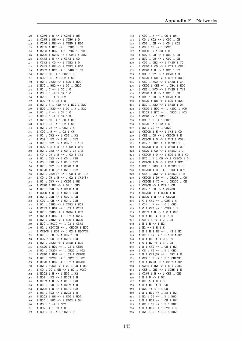
Appendix E. Networks
120 1 C2H6 1 O -> 1 C2H5 1 OH
121 1 C2H5 1 OH -> 1 C2H6 1 O
122 1 C2H6 1 OH -> 1 C2H5 1 H2O
123 1 C2H5 1 H2O -> 1 C2H6 1 OH
124 1 C2H6 1 HO2 -> 1 H2O2 1 C2H5
125 1 H2O2 1 C2H5 -> 1 C2H6 1 HO2
126 1 C4H2 1 O -> 1 C3H2 1 CO
127 1 C3H2 1 CO -> 1 C4H2 1 O
128 1 C4H2 1 OH -> 1 C3H2 1 HCO
129 1 C3H2 1 HCO -> 1 C4H2 1 OH
130 1 O2 1 CO -> 1 CO2 1 O
131 1 CO2 1 O -> 1 O2 1 CO
132 1 O2 1 CH2O -> 1 HCO 1 HO2
133 1 HCO 1 HO2 -> 1 O2 1 CH2O
134 1 O2 1 C -> 1 CO 1 O
135 1 CO 1 O -> 1 O2 1 C
136 1 O2 1 H -> 1 HO2
137 1 HO2 -> 1 O2 1 H
138 1 O2 1 H 1 H2O -> 1 HO2 1 H2O
139 1 HO2 1 H2O -> 1 O2 1 H 1 H2O
140 1 O2 1 H -> 1 OH 1 O
141 1 OH 1 O -> 1 O2 1 H
142 1 O2 1 CH -> 1 CO 1 OH
143 1 CO 1 OH -> 1 O2 1 CH
144 1 O2 1 CH -> 1 CO2 1 H
145 1 CO2 1 H -> 1 O2 1 CH
146 1 O2 1 CH2 -> 1 CO2 1 H2
147 1 CO2 1 H2 -> 1 O2 1 CH2
148 1 O2 1 CH2 -> 1 CO2 1 H 1 H
149 1 CO2 1 H 1 H -> 1 O2 1 CH2
150 1 O2 1 CH2 -> 1 CO 1 OH 1 H
151 1 CO 1 OH 1 H -> 1 O2 1 CH2
152 1 O2 1 CH2 -> 1 CO 1 H2O
153 1 CO 1 H2O -> 1 O2 1 CH2
154 1 O2 1 CH2 -> 1 CH2O 1 O
155 1 CH2O 1 O -> 1 O2 1 CH2
156 1 O2 1 CH2(S) -> 1 CO 1 OH 1 H
157 1 CO 1 OH 1 H -> 1 O2 1 CH2(S)
158 1 O2 1 CH3 -> 1 CH2O 1 OH
159 1 CH2O 1 OH -> 1 O2 1 CH3
160 1 O2 1 C2H -> 1 HCCO 1 O
161 1 HCCO 1 O -> 1 O2 1 C2H
162 1 O2 1 C2H -> 1 CO2 1 CH
163 1 CO2 1 CH -> 1 O2 1 C2H
164 1 O2 1 C2H3 -> 1 C2H2 1 HO2
165 1 C2H2 1 HO2 -> 1 O2 1 C2H3
166 1 O2 1 C2H5 -> 1 C2H4 1 HO2
167 1 C2H4 1 HO2 -> 1 O2 1 C2H5
168 1 O2 1 C3H2 -> 1 HCO 1 HCCO
169 1 HCO 1 HCCO -> 1 O2 1 C3H2
170 1 O2 1 H2CCCH -> 1 CH2CO 1 HCO
171 1 CH2CO 1 HCO -> 1 O2 1 H2CCCH
172 1 O2 1 HCO -> 1 HO2 1 CO
173 1 HO2 1 CO -> 1 O2 1 HCO
174 1 O2 1 CH3O -> 1 CH2O 1 HO2
175 1 CH2O 1 HO2 -> 1 O2 1 CH3O
176 1 O2 1 CH2OH -> 1 CH2O 1 HO2
177 1 CH2O 1 HO2 -> 1 O2 1 CH2OH
178 1 O2 1 CH2OH -> 1 CH2O 1 HO2
179 1 CH2O 1 HO2 -> 1 O2 1 CH2OH
180 1 O2 1 HCCO -> 1 CO 1 CO 1 OH
181 1 CO 1 CO 1 OH -> 1 O2 1 HCCO
182 1 H2O2 1 H -> 1 HO2 1 H2
183 1 HO2 1 H2 -> 1 H2O2 1 H
184 1 H2O2 1 H -> 1 OH 1 H2O
185 1 OH 1 H2O -> 1 H2O2 1 H
186 1 H2O2 1 O -> 1 OH 1 HO2
187 1 OH 1 HO2 -> 1 H2O2 1 O
188 1 H2O2 1 OH -> 1 H2O 1 HO2
189 1 H2O 1 HO2 -> 1 H2O2 1 OH
190 1 CO 1 O -> 1 CO2
191 1 CO2 -> 1 CO 1 O
192 1 CO 1 OH -> 1 CO2 1 H
193 1 CO2 1 H -> 1 CO 1 OH
194 1 CO 1 HO2 -> 1 CO2 1 OH
195 1 CO2 1 OH -> 1 CO 1 HO2
196 1 CO 1 CH -> 1 HCCO
197 1 HCCO -> 1 CO 1 CH
198 1 CO2 1 CH -> 1 HCO 1 CO
199 1 HCO 1 CO -> 1 CO2 1 CH
200 1 CO2 1 CH2 -> 1 CH2O 1 CO
201 1 CH2O 1 CO -> 1 CO2 1 CH2
202 1 CH2O 1 H -> 1 HCO 1 H2
203 1 HCO 1 H2 -> 1 CH2O 1 H
204 1 CH2O 1 CH -> 1 CH2 1 HCO
205 1 CH2 1 HCO -> 1 CH2O 1 CH
206 1 CH2O 1 CH3 -> 1 CH4 1 HCO
207 1 CH4 1 HCO -> 1 CH2O 1 CH3
208 1 CH2O 1 O -> 1 HCO 1 OH
209 1 HCO 1 OH -> 1 CH2O 1 O
210 1 CH2O 1 OH -> 1 HCO 1 H2O
211 1 HCO 1 H2O -> 1 CH2O 1 OH
212 1 CH2O 1 HO2 -> 1 H2O2 1 HCO
213 1 H2O2 1 HCO -> 1 CH2O 1 HO2
214 1 CH2O -> 1 HCO 1 H
215 1 HCO 1 H -> 1 CH2O
216 1 CH2O -> 1 H2 1 CO
217 1 H2 1 CO -> 1 CH2O
218 1 CH2CO 1 H -> 1 CH3 1 CO
219 1 CH3 1 CO -> 1 CH2CO 1 H
220 1 CH2CO 1 O -> 1 CH2 1 CO2
221 1 CH2 1 CO2 -> 1 CH2CO 1 O
222 1 CH2CO 1 O -> 1 CH2O 1 CO
223 1 CH2O 1 CO -> 1 CH2CO 1 O
224 1 CH2CO 1 O -> 1 HCO 1 H 1 CO
225 1 HCO 1 H 1 CO -> 1 CH2CO 1 O
226 1 CH2CO 1 O -> 1 HCO 1 HCO
227 1 HCO 1 HCO -> 1 CH2CO 1 O
228 1 CH2CO 1 OH -> 1 CH3 1 CO2
229 1 CH3 1 CO2 -> 1 CH2CO 1 OH
230 1 CH2CO 1 OH -> 1 CH2OH 1 CO
231 1 CH2OH 1 CO -> 1 CH2CO 1 OH
232 1 CH2CO -> 1 CH2 1 CO
233 1 CH2 1 CO -> 1 CH2CO
234 1 CH2CO -> 1 HCCO 1 H
235 1 HCCO 1 H -> 1 CH2CO
236 1 C 1 CH2 -> 1 C2H 1 H
237 1 C2H 1 H -> 1 C 1 CH2
238 1 C 1 CH3 -> 1 C2H2 1 H
239 1 C2H2 1 H -> 1 C 1 CH3
240 1 C 1 OH -> 1 CO 1 H
241 1 CO 1 H -> 1 C 1 OH
242 1 H 1 H -> 1 H2
243 1 H2 -> 1 H 1 H
244 1 H 1 H 1 H2 -> 1 H2 1 H2
245 1 H2 1 H2 -> 1 H 1 H 1 H2
246 1 H 1 CH -> 1 C 1 H2
247 1 C 1 H2 -> 1 H 1 CH
248 1 H 1 CH2 -> 1 CH 1 H2
249 1 CH 1 H2 -> 1 H 1 CH2
250 1 H 1 CH2(S) -> 1 CH2 1 H
251 1 CH2 1 H -> 1 H 1 CH2(S)
252 1 H 1 C2H3 -> 1 C2H2 1 H2
253 1 C2H2 1 H2 -> 1 H 1 C2H3
254 1 CH3 1 CH3 -> 1 C2H5 1 H
255 1 C2H5 1 H -> 1 CH3 1 CH3
256 1 H 1 O -> 1 OH
257 1 OH -> 1 H 1 O
258 1 H 1 OH -> 1 H2O
259 1 H2O -> 1 H 1 OH
260 1 H 1 HO2 -> 1 H2 1 O2
261 1 H2 1 O2 -> 1 H 1 HO2
262 1 H 1 HO2 -> 1 OH 1 OH
263 1 OH 1 OH -> 1 H 1 HO2
264 1 H 1 HO2 -> 1 H2O 1 O
265 1 H2O 1 O -> 1 H 1 HO2
145
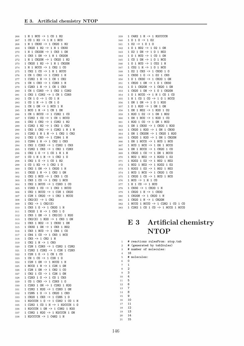
E 3. Artificial chemistry NTOP
266 1 H 1 HCO -> 1 CO 1 H2
267 1 CO 1 H2 -> 1 H 1 HCO
268 1 H 1 CH3O -> 1 CH2O 1 H2
269 1 CH2O 1 H2 -> 1 H 1 CH3O
270 1 H 1 CH2OH -> 1 CH3 1 OH
271 1 CH3 1 OH -> 1 H 1 CH2OH
272 1 H 1 CH2OH -> 1 CH2O 1 H2
273 1 CH2O 1 H2 -> 1 H 1 CH2OH
274 1 H 1 HCCO -> 1 CH2 1 CO
275 1 CH2 1 CO -> 1 H 1 HCCO
276 1 CH 1 CH2 -> 1 C2H2 1 H
277 1 C2H2 1 H -> 1 CH 1 CH2
278 1 CH 1 CH3 -> 1 C2H3 1 H
279 1 C2H3 1 H -> 1 CH 1 CH3
280 1 CH 1 C2H3 -> 1 CH2 1 C2H2
281 1 CH2 1 C2H2 -> 1 CH 1 C2H3
282 1 CH 1 O -> 1 CO 1 H
283 1 CO 1 H -> 1 CH 1 O
284 1 CH 1 OH -> 1 HCO 1 H
285 1 HCO 1 H -> 1 CH 1 OH
286 1 CH 1 HCCO -> 1 C2H2 1 CO
287 1 C2H2 1 CO -> 1 CH 1 HCCO
288 1 CH2 1 CH2 -> 1 C2H2 1 H2
289 1 C2H2 1 H2 -> 1 CH2 1 CH2
290 1 CH2 1 CH2 -> 1 C2H2 1 H 1 H
291 1 C2H2 1 H 1 H -> 1 CH2 1 CH2
292 1 CH2 1 CH3 -> 1 C2H4 1 H
293 1 C2H4 1 H -> 1 CH2 1 CH3
294 1 CH2 1 C2H3 -> 1 C2H2 1 CH3
295 1 C2H2 1 CH3 -> 1 CH2 1 C2H3
296 1 CH2 1 O -> 1 CO 1 H 1 H
297 1 CO 1 H 1 H -> 1 CH2 1 O
298 1 CH2 1 O -> 1 CO 1 H2
299 1 CO 1 H2 -> 1 CH2 1 O
300 1 CH2 1 OH -> 1 CH2O 1 H
301 1 CH2O 1 H -> 1 CH2 1 OH
302 1 CH2 1 HCO -> 1 CH3 1 CO
303 1 CH3 1 CO -> 1 CH2 1 HCO
304 1 CH2 1 HCCO -> 1 C2H3 1 CO
305 1 C2H3 1 CO -> 1 CH2 1 HCCO
306 1 CH2 1 HCCO -> 1 C2H 1 CH2O
307 1 C2H 1 CH2O -> 1 CH2 1 HCCO
308 1 CH2(S) -> 1 CH2
309 1 CH2 -> 1 CH2(S)
310 1 CH3 1 O -> 1 CH2O 1 H
311 1 CH2O 1 H -> 1 CH3 1 O
312 1 CH3 1 OH -> 1 CH2(S) 1 H2O
313 1 CH2(S) 1 H2O -> 1 CH3 1 OH
314 1 CH3 1 HO2 -> 1 CH3O 1 OH
315 1 CH3O 1 OH -> 1 CH3 1 HO2
316 1 CH3 1 HCO -> 1 CH4 1 CO
317 1 CH4 1 CO -> 1 CH3 1 HCO
318 1 CH3 -> 1 CH2 1 H
319 1 CH2 1 H -> 1 CH3
320 1 C2H 1 C2H3 -> 1 C2H2 1 C2H2
321 1 C2H2 1 C2H2 -> 1 C2H 1 C2H3
322 1 C2H 1 O -> 1 CH 1 CO
323 1 CH 1 CO -> 1 C2H 1 O
324 1 C2H 1 OH -> 1 HCCO 1 H
325 1 HCCO 1 H -> 1 C2H 1 OH
326 1 C2H 1 OH -> 1 CH2 1 CO
327 1 CH2 1 CO -> 1 C2H 1 OH
328 1 C2H3 1 O -> 1 CO 1 CH3
329 1 CO 1 CH3 -> 1 C2H3 1 O
330 1 C2H3 1 OH -> 1 C2H2 1 H2O
331 1 C2H2 1 H2O -> 1 C2H3 1 OH
332 1 C2H5 1 O -> 1 CH2O 1 CH3
333 1 CH2O 1 CH3 -> 1 C2H5 1 O
334 1 H2CCCH 1 O -> 1 C2H2 1 CO 1 H
335 1 C2H2 1 CO 1 H -> 1 H2CCCH 1 O
336 1 H2CCCH 1 OH -> 1 C3H2 1 H2O
337 1 C3H2 1 H2O -> 1 H2CCCH 1 OH
338 1 H2CCCCH -> 1 C4H2 1 H
339 1 C4H2 1 H -> 1 H2CCCCH
340 1 O 1 O -> 1 O2
341 1 O2 -> 1 O 1 O
342 1 O 1 HO2 -> 1 O2 1 OH
343 1 O2 1 OH -> 1 O 1 HO2
344 1 O 1 HCO -> 1 CO 1 OH
345 1 CO 1 OH -> 1 O 1 HCO
346 1 O 1 HCO -> 1 CO2 1 H
347 1 CO2 1 H -> 1 O 1 HCO
348 1 O2 1 CH3 -> 1 CH3O 1 O
349 1 CH3O 1 O -> 1 O2 1 CH3
350 1 O 1 CH3O -> 1 CH2O 1 OH
351 1 CH2O 1 OH -> 1 O 1 CH3O
352 1 O 1 CH2OH -> 1 CH2O 1 OH
353 1 CH2O 1 OH -> 1 O 1 CH2OH
354 1 O 1 HCCO -> 1 H 1 CO 1 CO
355 1 H 1 CO 1 CO -> 1 O 1 HCCO
356 1 OH 1 OH -> 1 O 1 H2O
357 1 O 1 H2O -> 1 OH 1 OH
358 1 OH 1 HO2 -> 1 H2O 1 O2
359 1 H2O 1 O2 -> 1 OH 1 HO2
360 1 OH 1 HCO -> 1 H2O 1 CO
361 1 H2O 1 CO -> 1 OH 1 HCO
362 1 OH 1 CH3O -> 1 CH2O 1 H2O
363 1 CH2O 1 H2O -> 1 OH 1 CH3O
364 1 OH 1 CH2OH -> 1 CH2O 1 H2O
365 1 CH2O 1 H2O -> 1 OH 1 CH2OH
366 1 OH 1 HCCO -> 1 HCO 1 HCO
367 1 HCO 1 HCO -> 1 OH 1 HCCO
368 1 OH 1 HCCO -> 1 CH2O 1 CO
369 1 CH2O 1 CO -> 1 OH 1 HCCO
370 1 HO2 1 HO2 -> 1 H2O2 1 O2
371 1 H2O2 1 O2 -> 1 HO2 1 HO2
372 1 HO2 1 HO2 -> 1 H2O2 1 O2
373 1 H2O2 1 O2 -> 1 HO2 1 HO2
374 1 HCO 1 HCO -> 1 CH2O 1 CO
375 1 CH2O 1 CO -> 1 HCO 1 HCO
376 1 HCO -> 1 H 1 CO
377 1 H 1 CO -> 1 HCO
378 1 CH3O -> 1 CH2O 1 H
379 1 CH2O 1 H -> 1 CH3O
380 1 CH2OH -> 1 CH2O 1 H
381 1 CH2O 1 H -> 1 CH2OH
382 1 HCCO 1 HCCO -> 1 C2H2 1 CO 1 CO
383 1 C2H2 1 CO 1 CO -> 1 HCCO 1 HCCO
E 3 Artificial chemistry
NTOP1 # reactions rulesFrom: ntop.tab
2 # (generated by tab2rules)
3 # number of molecules:
4 16
5 # molecules:
6 0
7 1
8 2
9 3
10 4
11 5
12 6
13 7
14 8
15 9
16 10
17 11
18 12
19 13
20 14
21 15
146
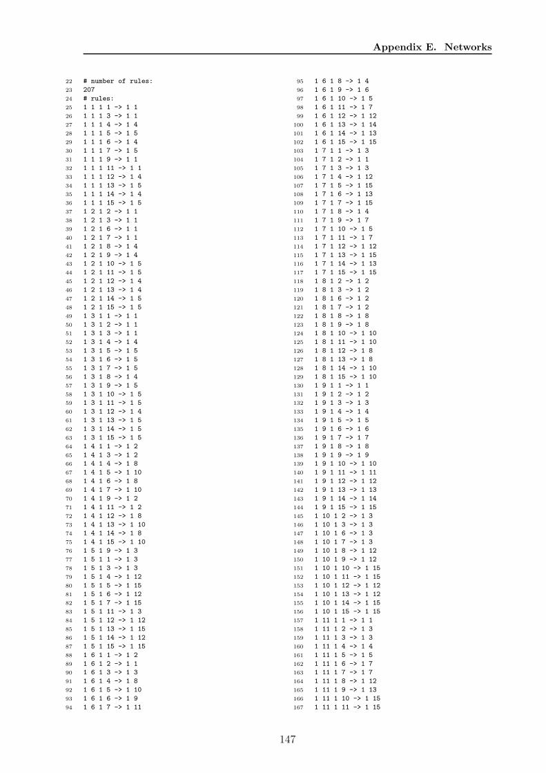
Appendix E. Networks
22 # number of rules:
23 207
24 # rules:
25 1 1 1 1 -> 1 1
26 1 1 1 3 -> 1 1
27 1 1 1 4 -> 1 4
28 1 1 1 5 -> 1 5
29 1 1 1 6 -> 1 4
30 1 1 1 7 -> 1 5
31 1 1 1 9 -> 1 1
32 1 1 1 11 -> 1 1
33 1 1 1 12 -> 1 4
34 1 1 1 13 -> 1 5
35 1 1 1 14 -> 1 4
36 1 1 1 15 -> 1 5
37 1 2 1 2 -> 1 1
38 1 2 1 3 -> 1 1
39 1 2 1 6 -> 1 1
40 1 2 1 7 -> 1 1
41 1 2 1 8 -> 1 4
42 1 2 1 9 -> 1 4
43 1 2 1 10 -> 1 5
44 1 2 1 11 -> 1 5
45 1 2 1 12 -> 1 4
46 1 2 1 13 -> 1 4
47 1 2 1 14 -> 1 5
48 1 2 1 15 -> 1 5
49 1 3 1 1 -> 1 1
50 1 3 1 2 -> 1 1
51 1 3 1 3 -> 1 1
52 1 3 1 4 -> 1 4
53 1 3 1 5 -> 1 5
54 1 3 1 6 -> 1 5
55 1 3 1 7 -> 1 5
56 1 3 1 8 -> 1 4
57 1 3 1 9 -> 1 5
58 1 3 1 10 -> 1 5
59 1 3 1 11 -> 1 5
60 1 3 1 12 -> 1 4
61 1 3 1 13 -> 1 5
62 1 3 1 14 -> 1 5
63 1 3 1 15 -> 1 5
64 1 4 1 1 -> 1 2
65 1 4 1 3 -> 1 2
66 1 4 1 4 -> 1 8
67 1 4 1 5 -> 1 10
68 1 4 1 6 -> 1 8
69 1 4 1 7 -> 1 10
70 1 4 1 9 -> 1 2
71 1 4 1 11 -> 1 2
72 1 4 1 12 -> 1 8
73 1 4 1 13 -> 1 10
74 1 4 1 14 -> 1 8
75 1 4 1 15 -> 1 10
76 1 5 1 9 -> 1 3
77 1 5 1 1 -> 1 3
78 1 5 1 3 -> 1 3
79 1 5 1 4 -> 1 12
80 1 5 1 5 -> 1 15
81 1 5 1 6 -> 1 12
82 1 5 1 7 -> 1 15
83 1 5 1 11 -> 1 3
84 1 5 1 12 -> 1 12
85 1 5 1 13 -> 1 15
86 1 5 1 14 -> 1 12
87 1 5 1 15 -> 1 15
88 1 6 1 1 -> 1 2
89 1 6 1 2 -> 1 1
90 1 6 1 3 -> 1 3
91 1 6 1 4 -> 1 8
92 1 6 1 5 -> 1 10
93 1 6 1 6 -> 1 9
94 1 6 1 7 -> 1 11
95 1 6 1 8 -> 1 4
96 1 6 1 9 -> 1 6
97 1 6 1 10 -> 1 5
98 1 6 1 11 -> 1 7
99 1 6 1 12 -> 1 12
100 1 6 1 13 -> 1 14
101 1 6 1 14 -> 1 13
102 1 6 1 15 -> 1 15
103 1 7 1 1 -> 1 3
104 1 7 1 2 -> 1 1
105 1 7 1 3 -> 1 3
106 1 7 1 4 -> 1 12
107 1 7 1 5 -> 1 15
108 1 7 1 6 -> 1 13
109 1 7 1 7 -> 1 15
110 1 7 1 8 -> 1 4
111 1 7 1 9 -> 1 7
112 1 7 1 10 -> 1 5
113 1 7 1 11 -> 1 7
114 1 7 1 12 -> 1 12
115 1 7 1 13 -> 1 15
116 1 7 1 14 -> 1 13
117 1 7 1 15 -> 1 15
118 1 8 1 2 -> 1 2
119 1 8 1 3 -> 1 2
120 1 8 1 6 -> 1 2
121 1 8 1 7 -> 1 2
122 1 8 1 8 -> 1 8
123 1 8 1 9 -> 1 8
124 1 8 1 10 -> 1 10
125 1 8 1 11 -> 1 10
126 1 8 1 12 -> 1 8
127 1 8 1 13 -> 1 8
128 1 8 1 14 -> 1 10
129 1 8 1 15 -> 1 10
130 1 9 1 1 -> 1 1
131 1 9 1 2 -> 1 2
132 1 9 1 3 -> 1 3
133 1 9 1 4 -> 1 4
134 1 9 1 5 -> 1 5
135 1 9 1 6 -> 1 6
136 1 9 1 7 -> 1 7
137 1 9 1 8 -> 1 8
138 1 9 1 9 -> 1 9
139 1 9 1 10 -> 1 10
140 1 9 1 11 -> 1 11
141 1 9 1 12 -> 1 12
142 1 9 1 13 -> 1 13
143 1 9 1 14 -> 1 14
144 1 9 1 15 -> 1 15
145 1 10 1 2 -> 1 3
146 1 10 1 3 -> 1 3
147 1 10 1 6 -> 1 3
148 1 10 1 7 -> 1 3
149 1 10 1 8 -> 1 12
150 1 10 1 9 -> 1 12
151 1 10 1 10 -> 1 15
152 1 10 1 11 -> 1 15
153 1 10 1 12 -> 1 12
154 1 10 1 13 -> 1 12
155 1 10 1 14 -> 1 15
156 1 10 1 15 -> 1 15
157 1 11 1 1 -> 1 1
158 1 11 1 2 -> 1 3
159 1 11 1 3 -> 1 3
160 1 11 1 4 -> 1 4
161 1 11 1 5 -> 1 5
162 1 11 1 6 -> 1 7
163 1 11 1 7 -> 1 7
164 1 11 1 8 -> 1 12
165 1 11 1 9 -> 1 13
166 1 11 1 10 -> 1 15
167 1 11 1 11 -> 1 15
147
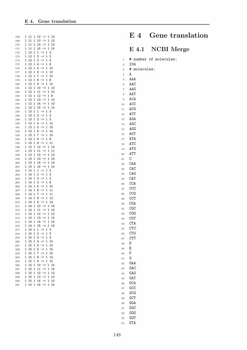
E 4. Gene translation
168 1 11 1 12 -> 1 12
169 1 11 1 13 -> 1 13
170 1 11 1 14 -> 1 15
171 1 11 1 15 -> 1 15
172 1 12 1 1 -> 1 2
173 1 12 1 2 -> 1 2
174 1 12 1 3 -> 1 2
175 1 12 1 4 -> 1 8
176 1 12 1 5 -> 1 10
177 1 12 1 6 -> 1 10
178 1 12 1 7 -> 1 10
179 1 12 1 8 -> 1 8
180 1 12 1 9 -> 1 10
181 1 12 1 10 -> 1 10
182 1 12 1 11 -> 1 10
183 1 12 1 12 -> 1 8
184 1 12 1 13 -> 1 10
185 1 12 1 14 -> 1 10
186 1 12 1 15 -> 1 10
187 1 13 1 1 -> 1 3
188 1 13 1 2 -> 1 2
189 1 13 1 3 -> 1 3
190 1 13 1 4 -> 1 12
191 1 13 1 5 -> 1 15
192 1 13 1 6 -> 1 14
193 1 13 1 7 -> 1 15
194 1 13 1 8 -> 1 8
195 1 13 1 9 -> 1 11
196 1 13 1 10 -> 1 10
197 1 13 1 11 -> 1 11
198 1 13 1 12 -> 1 12
199 1 13 1 13 -> 1 15
200 1 13 1 14 -> 1 14
201 1 13 1 15 -> 1 15
202 1 14 1 1 -> 1 2
203 1 14 1 2 -> 1 3
204 1 14 1 3 -> 1 3
205 1 14 1 4 -> 1 8
206 1 14 1 5 -> 1 10
207 1 14 1 6 -> 1 11
208 1 14 1 7 -> 1 11
209 1 14 1 8 -> 1 12
210 1 14 1 9 -> 1 14
211 1 14 1 10 -> 1 15
212 1 14 1 11 -> 1 15
213 1 14 1 12 -> 1 12
214 1 14 1 13 -> 1 14
215 1 14 1 14 -> 1 15
216 1 14 1 15 -> 1 15
217 1 15 1 1 -> 1 3
218 1 15 1 2 -> 1 3
219 1 15 1 3 -> 1 3
220 1 15 1 4 -> 1 12
221 1 15 1 5 -> 1 15
222 1 15 1 6 -> 1 15
223 1 15 1 7 -> 1 15
224 1 15 1 8 -> 1 12
225 1 15 1 9 -> 1 15
226 1 15 1 10 -> 1 15
227 1 15 1 11 -> 1 15
228 1 15 1 12 -> 1 12
229 1 15 1 13 -> 1 15
230 1 15 1 14 -> 1 15
231 1 15 1 15 -> 1 15
E 4 Gene translation
E 4.1 NCBI Merge
1 # number of molecules:
2 234
3 # molecules:
4 A
5 AAA
6 AAC
7 AAG
8 AAT
9 ACA
10 ACC
11 ACG
12 ACT
13 AGA
14 AGC
15 AGG
16 AGT
17 ATA
18 ATC
19 ATG
20 ATT
21 C
22 CAA
23 CAC
24 CAG
25 CAT
26 CCA
27 CCC
28 CCG
29 CCT
30 CGA
31 CGC
32 CGG
33 CGT
34 CTA
35 CTC
36 CTG
37 CTT
38 D
39 E
40 F
41 G
42 GAA
43 GAC
44 GAG
45 GAT
46 GCA
47 GCC
48 GCG
49 GCT
50 GGA
51 GGC
52 GGG
53 GGT
54 GTA
148
Appendix E. Networks
55 GTC
56 GTG
57 GTT
58 H
59 I
60 K
61 L
62 M
63 N
64 O
65 P
66 Q
67 R
68 S
69 T
70 TAA
71 TAC
72 TAG
73 TAT
74 TCA
75 TCC
76 TCG
77 TCT
78 TGA
79 TGC
80 TGG
81 TGT
82 TTA
83 TTC
84 TTG
85 TTT
86 V
87 W
88 Y
89 tRNAAAA
90 tRNAAAAK
91 tRNAAAAN
92 tRNAAAC
93 tRNAAACN
94 tRNAAAG
95 tRNAAAGK
96 tRNAAAT
97 tRNAAATN
98 tRNAACA
99 tRNAACAT
100 tRNAACC
101 tRNAACCT
102 tRNAACG
103 tRNAACGT
104 tRNAACT
105 tRNAACTT
106 tRNAAGA
107 tRNAAGAG
108 tRNAAGAO
109 tRNAAGAR
110 tRNAAGAS
111 tRNAAGC
112 tRNAAGCS
113 tRNAAGG
114 tRNAAGGG
115 tRNAAGGO
116 tRNAAGGR
117 tRNAAGGS
118 tRNAAGT
119 tRNAAGTS
120 tRNAATA
121 tRNAATAI
122 tRNAATAM
123 tRNAATC
124 tRNAATCI
125 tRNAATG
126 tRNAATGM
127 tRNAATT
128 tRNAATTI
129 tRNACAA
130 tRNACAAQ
131 tRNACAC
132 tRNACACH
133 tRNACAG
134 tRNACAGQ
135 tRNACAT
136 tRNACATH
137 tRNACCA
138 tRNACCAP
139 tRNACCC
140 tRNACCCP
141 tRNACCG
142 tRNACCGP
143 tRNACCT
144 tRNACCTP
145 tRNACGA
146 tRNACGAR
147 tRNACGC
148 tRNACGCR
149 tRNACGG
150 tRNACGGR
151 tRNACGT
152 tRNACGTR
153 tRNACTA
154 tRNACTAL
155 tRNACTAT
156 tRNACTC
157 tRNACTCL
158 tRNACTCT
159 tRNACTG
160 tRNACTGL
161 tRNACTGS
162 tRNACTGT
163 tRNACTT
164 tRNACTTL
165 tRNACTTT
166 tRNAGAA
167 tRNAGAAE
168 tRNAGAC
169 tRNAGACD
170 tRNAGAG
149

E 4. Gene translation
171 tRNAGAGE
172 tRNAGAT
173 tRNAGATD
174 tRNAGCA
175 tRNAGCAA
176 tRNAGCC
177 tRNAGCCA
178 tRNAGCG
179 tRNAGCGA
180 tRNAGCT
181 tRNAGCTA
182 tRNAGGA
183 tRNAGGAG
184 tRNAGGC
185 tRNAGGCG
186 tRNAGGG
187 tRNAGGGG
188 tRNAGGT
189 tRNAGGTG
190 tRNAGTA
191 tRNAGTAV
192 tRNAGTC
193 tRNAGTCV
194 tRNAGTG
195 tRNAGTGV
196 tRNAGTT
197 tRNAGTTV
198 tRNATAA
199 tRNATAAO
200 tRNATAAQ
201 tRNATAAY
202 tRNATAC
203 tRNATACY
204 tRNATAG
205 tRNATAGL
206 tRNATAGO
207 tRNATAGQ
208 tRNATAT
209 tRNATATY
210 tRNATCA
211 tRNATCAO
212 tRNATCAS
213 tRNATCC
214 tRNATCCS
215 tRNATCG
216 tRNATCGS
217 tRNATCT
218 tRNATCTS
219 tRNATGA
220 tRNATGAC
221 tRNATGAO
222 tRNATGAW
223 tRNATGC
224 tRNATGCC
225 tRNATGG
226 tRNATGGW
227 tRNATGT
228 tRNATGTC
229 tRNATTA
230 tRNATTAL
231 tRNATTAO
232 tRNATTC
233 tRNATTCF
234 tRNATTG
235 tRNATTGL
236 tRNATTT
237 tRNATTTF
238 # number of rules:
239 85
240 # rules:
241 1 CTG 1 tRNACTGT -> 1 T
242 1 GAC 1 tRNAGACD -> 1 D
243 1 TAG 1 tRNATAGO -> 1 O
244 1 TAC 1 tRNATACY -> 1 Y
245 1 CTC 1 tRNACTCL -> 1 L
246 1 GAG 1 tRNAGAGE -> 1 E
247 1 GTA 1 tRNAGTAV -> 1 V
248 1 AGG 1 tRNAAGGG -> 1 G
249 1 AGA 1 tRNAAGAO -> 1 O
250 1 TCC 1 tRNATCCS -> 1 S
251 1 AGT 1 tRNAAGTS -> 1 S
252 1 TAG 1 tRNATAGQ -> 1 Q
253 1 ACA 1 tRNAACAT -> 1 T
254 1 GCG 1 tRNAGCGA -> 1 A
255 1 CTC 1 tRNACTCT -> 1 T
256 1 CCC 1 tRNACCCP -> 1 P
257 1 TAA 1 tRNATAAO -> 1 O
258 1 CTT 1 tRNACTTL -> 1 L
259 1 CTG 1 tRNACTGS -> 1 S
260 1 TTT 1 tRNATTTF -> 1 F
261 1 GGT 1 tRNAGGTG -> 1 G
262 1 GAT 1 tRNAGATD -> 1 D
263 1 CGG 1 tRNACGGR -> 1 R
264 1 ATT 1 tRNAATTI -> 1 I
265 1 CTG 1 tRNACTGL -> 1 L
266 1 ATA 1 tRNAATAI -> 1 I
267 1 ACT 1 tRNAACTT -> 1 T
268 1 GTT 1 tRNAGTTV -> 1 V
269 1 GCT 1 tRNAGCTA -> 1 A
270 1 GCA 1 tRNAGCAA -> 1 A
271 1 TAA 1 tRNATAAY -> 1 Y
272 1 CAT 1 tRNACATH -> 1 H
273 1 ATA 1 tRNAATAM -> 1 M
274 1 TCG 1 tRNATCGS -> 1 S
275 1 ATG 1 tRNAATGM -> 1 M
276 1 TGA 1 tRNATGAW -> 1 W
277 1 GAA 1 tRNAGAAE -> 1 E
278 1 AAA 1 tRNAAAAN -> 1 N
279 1 TCA 1 tRNATCAS -> 1 S
280 1 AAA 1 tRNAAAAK -> 1 K
281 1 TCA 1 tRNATCAO -> 1 O
282 1 TAT 1 tRNATATY -> 1 Y
283 1 TGA 1 tRNATGAC -> 1 C
284 1 AGA 1 tRNAAGAR -> 1 R
285 1 CTA 1 tRNACTAL -> 1 L
286 1 AGA 1 tRNAAGAS -> 1 S
150
Appendix E. Networks
287 1 TGT 1 tRNATGTC -> 1 C
288 1 CTA 1 tRNACTAT -> 1 T
289 1 TTC 1 tRNATTCF -> 1 F
290 1 CCT 1 tRNACCTP -> 1 P
291 1 CGT 1 tRNACGTR -> 1 R
292 1 CGA 1 tRNACGAR -> 1 R
293 1 TGC 1 tRNATGCC -> 1 C
294 1 CCA 1 tRNACCAP -> 1 P
295 1 AAG 1 tRNAAAGK -> 1 K
296 1 GCC 1 tRNAGCCA -> 1 A
297 1 CAG 1 tRNACAGQ -> 1 Q
298 1 TGA 1 tRNATGAO -> 1 O
299 1 GTC 1 tRNAGTCV -> 1 V
300 1 AGA 1 tRNAAGAG -> 1 G
301 1 TTG 1 tRNATTGL -> 1 L
302 1 TCT 1 tRNATCTS -> 1 S
303 1 ACG 1 tRNAACGT -> 1 T
304 1 TGG 1 tRNATGGW -> 1 W
305 1 AAC 1 tRNAAACN -> 1 N
306 1 GGG 1 tRNAGGGG -> 1 G
307 1 CAA 1 tRNACAAQ -> 1 Q
308 1 TAA 1 tRNATAAQ -> 1 Q
309 1 AGG 1 tRNAAGGR -> 1 R
310 1 TTA 1 tRNATTAO -> 1 O
311 1 AGG 1 tRNAAGGS -> 1 S
312 1 TAG 1 tRNATAGL -> 1 L
313 1 ACC 1 tRNAACCT -> 1 T
314 1 GGC 1 tRNAGGCG -> 1 G
315 1 AAT 1 tRNAAATN -> 1 N
316 1 GGA 1 tRNAGGAG -> 1 G
317 1 CTT 1 tRNACTTT -> 1 T
318 1 CCG 1 tRNACCGP -> 1 P
319 1 CGC 1 tRNACGCR -> 1 R
320 1 AGC 1 tRNAAGCS -> 1 S
321 1 CAC 1 tRNACACH -> 1 H
322 1 GTG 1 tRNAGTGV -> 1 V
323 1 TTA 1 tRNATTAL -> 1 L
324 1 ATC 1 tRNAATCI -> 1 I
325 1 AGG 1 tRNAAGGO -> 1 O
E 4.2 Completed GC w/o
synthetases (excerpt)1 # number of molecules:
2 1364
3 # molecules:
4 C1
5 C2
6 ...
7 C63
8 C64
9 AAprot1
10 AAprot2
11 ...
12 AAprot19
13 AAprot20
14 tRNA11
15 tRNA12
16 ...
17 tRNA641
18 tRNA642
19 tRNA643
20 tRNA644
21 tRNA645
22 tRNA646
23 tRNA647
24 tRNA648
25 tRNA649
26 tRNA6410
27 tRNA6411
28 tRNA6412
29 tRNA6413
30 tRNA6414
31 tRNA6415
32 tRNA6416
33 tRNA6417
34 tRNA6418
35 tRNA6419
36 tRNA6420
37 # number of rules:
38 1280
39 # rules:
40 1 tRNA11 1 C1 -> 1 C1 1 AAprot1
41 1 tRNA12 1 C1 -> 1 C1 1 AAprot2
42 ...
43 1 tRNA6410 1 C64 -> 1 C64 1 AAprot10
44 1 tRNA6411 1 C64 -> 1 C64 1 AAprot11
45 1 tRNA6412 1 C64 -> 1 C64 1 AAprot12
46 1 tRNA6413 1 C64 -> 1 C64 1 AAprot13
47 1 tRNA6414 1 C64 -> 1 C64 1 AAprot14
48 1 tRNA6415 1 C64 -> 1 C64 1 AAprot15
49 1 tRNA6416 1 C64 -> 1 C64 1 AAprot16
50 1 tRNA6417 1 C64 -> 1 C64 1 AAprot17
51 1 tRNA6418 1 C64 -> 1 C64 1 AAprot18
52 1 tRNA6419 1 C64 -> 1 C64 1 AAprot19
53 1 tRNA6420 1 C64 -> 1 C64 1 AAprot20
E 4.3 Complete GC withsynthetases (excerpt)
1 # number of molecules:
2 2728
3 # molecules:
4 C1
5 tRNA1
6 C2
7 tRNA2
8 ...
9 C63
10 tRNA63
11 C64
12 tRNA64
13 AA1-free
14 AA1-prot
15 AA2-free
16 AA2-prot
17 ...
18 AA19-free
19 AA19-prot
20 AA20-free
21 AA20-prot
22 Syn_C1-AA1
23 AA1-tRNA1
24 Syn_C1-AA2
25 AA2-tRNA1
26 ...
27 Syn_C64-AA19
28 AA19-tRNA64
29 Syn_C64-AA20
30 AA20-tRNA64
31 # number of rules:
32 2560
151
E 6. Phosphorylation cascades
33 # rules:
34 1 AA1-free 1 tRNA1 1 Syn_C1-AA1
35 -> 1 Syn_C1-AA1 1 AA1-tRNA1
36 1 AA1-tRNA1 1 C1 -> 1 C1 1 AA1-prot 1 tRNA1
37 1 AA2-free 1 tRNA1 1 Syn_C1-AA2
38 -> 1 Syn_C1-AA2 1 AA2-tRNA1
39 1 AA2-tRNA1 1 C1 -> 1 C1 1 AA2-prot 1 tRNA1
40 ...
41 1 AA17-free 1 tRNA64 1 Syn_C64-AA17
42 -> 1 Syn_C64-AA17 1 AA17-tRNA64
43 1 AA17-tRNA64 1 C64 -> 1 C64 1 AA17-prot 1 tRNA64
44 1 AA18-free 1 tRNA64 1 Syn_C64-AA18
45 -> 1 Syn_C64-AA18 1 AA18-tRNA64
46 1 AA18-tRNA64 1 C64 -> 1 C64 1 AA18-prot 1 tRNA64
47 1 AA19-free 1 tRNA64 1 Syn_C64-AA19
48 -> 1 Syn_C64-AA19 1 AA19-tRNA64
49 1 AA19-tRNA64 1 C64 -> 1 C64 1 AA19-prot 1 tRNA64
50 1 AA20-free 1 tRNA64 1 Syn_C64-AA20
51 -> 1 Syn_C64-AA20 1 AA20-tRNA64
52 1 AA20-tRNA64 1 C64 -> 1 C64 1 AA20-prot 1 tRNA64
E 5 Gene regulatory net-
works
E 5.1 GC-GRN network
1 # Number of Components:
2 14
3 # Components:
4 TF1
5 TF2
6 tRNAAL
7 tRNAAK
8 tRNABL
9 tRNABK
10 P1ABA
11 P2ABA
12 P1BAB
13 P2BAB
14 LKL
15 KLK
16 LLL
17 KKK
18 # Number of Reactions:
19 16
20 # Reactions:
21 1 TF1 1 P1ABA 1 tRNAAL 1 tRNABK -> 1 LKL
22 1 TF1 1 P1ABA 1 tRNAAL 1 tRNABL -> 1 LLL
23 1 TF1 1 P1ABA 1 tRNAAK 1 tRNABK -> 1 KKK
24 1 TF1 1 P1ABA 1 tRNAAK 1 tRNABL -> 1 KLK
25 1 TF1 1 P1BAB 1 tRNAAL 1 tRNABK -> 1 KLK
26 1 TF1 1 P1BAB 1 tRNAAL 1 tRNABL -> 1 LLL
27 1 TF1 1 P1BAB 1 tRNAAK 1 tRNABK -> 1 KKK
28 1 TF1 1 P1BAB 1 tRNAAK 1 tRNABL -> 1 LKL
29 1 TF2 1 P2ABA 1 tRNAAL 1 tRNABK -> 1 LKL
30 1 TF2 1 P2ABA 1 tRNAAL 1 tRNABL -> 1 LLL
31 1 TF2 1 P2ABA 1 tRNAAK 1 tRNABK -> 1 KKK
32 1 TF2 1 P2ABA 1 tRNAAK 1 tRNABL -> 1 KLK
33 1 TF2 1 P2BAB 1 tRNAAL 1 tRNABK -> 1 KLK
34 1 TF2 1 P2BAB 1 tRNAAL 1 tRNABL -> 1 LLL
35 1 TF2 1 P2BAB 1 tRNAAK 1 tRNABK -> 1 KKK
36 1 TF2 1 P2BAB 1 tRNAAK 1 tRNABL -> 1 LKL
E 5.2 Extended GC-GRN
network
1 # reactions extended GC GRN model
2 # number of molecules:
3 16
4 # molecules:
5 TF1
6 TF2
7 tRNAAL
8 tRNAAK
9 tRNABL
10 tRNABK
11 P1ABA
12 P2ABA
13 P1BAB
14 P2BAB
15 LKL
16 KLK
17 LLL
18 KKK
19 ABA
20 BAB
21 # number of rules:
22 10
23 # rules:
24 1 TF1 1 P1ABA -> 1 ABA
25 1 TF2 1 P2ABA -> 1 ABA
26 1 TF1 1 P1BAB -> 1 BAB
27 1 TF2 1 P2BAB -> 1 BAB
28 1 ABA 1 tRNAAL 1 tRNABK -> 1 LKL
29 1 ABA 1 tRNAAL 1 tRNABL -> 1 LLL
30 1 ABA 1 tRNAAK 1 tRNABK -> 1 KKK
31 1 BAB 1 tRNAAK 1 tRNABL -> 1 LKL
32 1 BAB 1 tRNAAL 1 tRNABK -> 1 KLK
33 1 BAB 1 tRNAAL 1 tRNABL -> 1 LLL
E 6 Phosphorylation cas-
cades
E 6.1 Simple phosphoryla-tion model
1 # Number of Components:
2 3
3 # Components:
4 A
5 AP
6 SP
7 # Number of Reactions:
8 2
152
Appendix E. Networks
9 # Reactions:
10 1 A 1 SP -> 1 AP 1 SP
11 1 AP -> 1 A
E 6.2 Extended phosphory-
lation model
1 # Number of Components:
2 7
3 # Components:
4 A
5 AP
6 B
7 BP
8 C
9 CP
10 SP
11 # Number of Reactions:
12 6
13 # Reactions:
14 1 B 1 SP -> 1 BP 1 SP
15 1 BP -> 1 B
16 1 C 1 SP -> 1 CP 1 SP
17 1 CP -> 1 C
18 1 A 1 B -> 1 AP
19 1 AP 1 CP -> 1 A
E 7 Protein assembly
E 7.1 Two steps, withoutdissociation
1 # Number of Components
2 20
3 # Components
4 A
5 B
6 AA
7 AB
8 BB
9 AAA
10 AAB
11 ABA
12 ABB
13 BAB
14 BBB
15 AAAA
16 AAAB
17 AABB
18 ABAA
19 ABAB
20 ABBA
21 ABBB
22 BBAB
23 BBBB
24 # Number of Reactions
25 20
26 # Reactions
27 1 A 1 A -> 1 AA
28 1 A 1 B -> 1 AB
29 1 B 1 B -> 1 BB
30 1 A 1 AA -> 1 AAA
31 1 A 1 AB -> 1 AAB
32 1 A 1 AB -> 1 ABA
33 1 A 1 BB -> 1 ABB
34 1 B 1 AA -> 1 AAB
35 1 B 1 AB -> 1 ABB
36 1 B 1 AB -> 1 BAB
37 1 B 1 BB -> 1 BBB
38 1 AA 1 AA -> 1 AAAA
39 1 AA 1 AB -> 1 AAAB
40 1 AA 1 AB -> 1 ABAA
41 1 AA 1 BB -> 1 AABB
42 1 AB 1 AB -> 1 ABAB
43 1 AB 1 AB -> 1 ABBA
44 1 BB 1 AB -> 1 ABBB
45 1 BB 1 AB -> 1 BBAB
46 1 BB 1 BB -> 1 BBBB
E 7.2 Two steps, with dis-sociation
1 # Number of Components
2 20
3 # Components
4 A
5 B
6 AA
7 AB
8 BB
9 AAA
10 AAB
11 ABA
12 ABB
13 BAB
14 BBB
15 AAAA
16 AAAB
17 AABB
18 ABAA
19 ABAB
20 ABBA
21 ABBB
22 BBAB
23 BBBB
24 # Number of Reactions
25 23
26 # Reactions
27 1 A 1 A -> 1 AA
28 1 AA -> 1 A 1 A
29 1 A 1 B -> 1 AB
30 1 AB -> 1 A 1 B
153
E 8. Photochemistry of Mars
31 1 B 1 B -> 1 BB
32 1 BB -> 1 B 1 B
33 1 A 1 AA -> 1 AAA
34 1 A 1 AB -> 1 AAB
35 1 A 1 AB -> 1 ABA
36 1 A 1 BB -> 1 ABB
37 1 B 1 AA -> 1 AAB
38 1 B 1 AB -> 1 ABB
39 1 B 1 AB -> 1 BAB
40 1 B 1 BB -> 1 BBB
41 1 AA 1 AA -> 1 AAAA
42 1 AA 1 AB -> 1 AAAB
43 1 AA 1 AB -> 1 ABAA
44 1 AA 1 BB -> 1 AABB
45 1 AB 1 AB -> 1 ABAB
46 1 AB 1 AB -> 1 ABBA
47 1 BB 1 AB -> 1 ABBB
48 1 BB 1 AB -> 1 BBAB
49 1 BB 1 BB -> 1 BBBB
E 8 Photochemistry of
Mars
1 # Number of Components
2 32
3 # Components
4 hv
5 M
6 e
7 O_3
8 O_2
9 O
10 O(^1D)
11 H_2
12 H
13 OH
14 HO_2
15 H_2O
16 H_2O_2
17 CO_2
18 CO
19 N_2
20 N
21 N(^2D)
22 NO
23 NO_2
24 NO_3
25 N_2O
26 N_2O_5
27 HNO_2
28 HNO_3
29 HO_2NO_2
30 O^+
31 O_2^+
32 CO_2^+
33 CO_2H^+
34 (HO_2)_grain
35 grain
36 # Number of Reactions
37 104
38 # Reactions
39 -> 1 hv
40 1 O_2 1 hv -> 2 O
41 1 O_2 1 hv -> 1 O 1 O(^1D)
42 1 O_3 1 hv -> 1 O_2 1 O
43 1 O_3 1 hv -> 1 O_2 1 O(^1D)
44 1 O_3 1 hv -> 3 O
45 1 H_2 1 hv -> 2 H
46 1 OH 1 hv -> 1 O 1 H
47 1 HO_2 1 hv -> 1 OH 1 O
48 1 H_2O 1 hv -> 1 H 1 OH
49 1 H_2O 1 hv -> 1 H_2 1 O(^1D)
50 1 H_2O 1 hv -> 2 H 1 O
51 1 H_2O_2 1 hv -> 2 OH
52 1 CO_2 1 hv -> 1 CO 1 O
53 1 CO_2 1 hv -> 1 CO 1 O(^1D)
54 2 O 1 M -> 1 O_2 1 M
55 1 O 1 O_2 1 N_2 -> 1 O_3 1 N_2
56 1 O 1 O_2 1 CO_2 -> 1 O_3 1 CO_2
57 1 O 1 O_3 -> 2 O_2
58 1 O 1 CO 1 M -> 1 CO_2 1 M
59 1 O(^1D) 1 O_2 -> 1 O 1 O_2
60 1 O(^1D) 1 O_3 -> 2 O_2
61 1 O(^1D) 1 O_3 -> 1 O_2 2 O
62 1 O(^1D) 1 H_2 -> 1 H 1 OH
63 1 O(^1D) 1 CO_2 -> 1 O 1 CO_2
64 1 O(^1D) 1 H_2O -> 2 OH
65 2 H 1 M -> 1 H_2 1 M
66 1 H 1 O_2 1 M -> 1 HO_2 1 M
67 1 H 1 O_3 -> 1 OH 1 O_2
68 1 H 1 HO_2 -> 2 OH
69 1 H 1 HO_2 -> 1 H_2 1 O_2
70 1 H 1 HO_2 -> 1 H_2O 1 O
71 1 O 1 H_2 -> 1 OH 1 H
72 1 O 1 OH -> 1 O_2 1 H
73 1 O 1 HO_2 -> 1 OH 1 O_2
74 1 O 1 H_2O_2 -> 1 OH 1 HO_2
75 2 OH -> 1 H_2O 1 O
76 2 OH 1 M -> 1 H_2O_2 1 M
77 1 OH 1 O_3 -> 1 HO_2 1 O_2
78 1 OH 1 H_2 -> 1 H_2O 1 H
79 1 OH 1 HO_2 -> 1 H_2O 1 O_2
80 1 OH 1 H_2O_2 -> 1 H_2O 1 HO_2
81 1 OH 1 CO -> 1 CO_2 1 H
82 1 HO_2 1 O_3 -> 1 OH 2 O_2
83 2 HO_2 -> 1 H_2O_2 1 O_2
84 2 HO_2 1 M -> 1 H_2O_2 1 O_2 1 M
85 1 N_2 -> 2 N
86 1 N_2 -> 2 N(^2D)
87 1 NO 1 hv -> 1 N 1 O
88 1 NO_2 1 hv -> 1 NO 1 O
89 1 NO_3 1 hv -> 1 NO_2 1 O
90 1 NO_3 1 hv -> 1 NO 1 O_2
91 1 N_2O 1 hv -> 1 N_2 1 O(^1D)
154
Appendix E. Networks
92 1 N_2O_5 1 hv -> 1 NO_2 1 NO_3
93 1 HNO_2 1 hv -> 1 OH 1 NO
94 1 HNO_3 1 hv -> 1 NO_2 1 OH
95 1 HO_2NO_2 1 hv -> 1 HO_2 1 NO_2
96 1 N 1 O_2 -> 1 NO 1 O
97 1 N 1 O_3 -> 1 NO 1 O_2
98 1 N 1 OH -> 1 NO 1 H
99 1 N 1 HO_2 -> 1 NO 1 OH
100 1 N 1 NO -> 1 N_2 1 O
101 1 N 1 NO_2 -> 1 N_2O 1 O
102 1 N(^2D) 1 O -> 1 N 1 O
103 1 N(^2D) 1 CO_2 -> 1 NO 1 CO
104 1 N(^2D) 1 N_2 -> 1 N 1 N_2
105 1 N(^2D) 1 NO -> 1 N_2 1 O
106 1 O 1 NO 1 M -> 1 NO_2 1 M
107 1 O 1 NO_2 -> 1 NO 1 O_2
108 1 O 1 NO_2 1 M -> 1 NO_3 1 M
109 1 O 1 NO_3 -> 1 O_2 1 NO_2
110 1 O 1 HO_2NO_2 -> 1 OH 1 NO_2 1 O_2
111 1 O(^1D) 1 N_2 -> 1 O 1 N_2
112 1 O(^1D) 1 N_2 1 M -> 1 N_2O 1 M
113 1 O(^1D) 1 N_2O -> 2 NO
114 1 O(^1D) 1 N_2O -> 1 N_2 1 O_2
115 1 NO 1 O_3 -> 1 NO_2 1 O_2
116 1 NO 1 HO_2 -> 1 NO_2 1 OH
117 1 NO 1 NO_3 -> 2 NO_2
118 1 H 1 NO_2 -> 1 OH 1 NO
119 1 H 1 NO_3 -> 1 OH 1 NO_2
120 1 OH 1 NO 1 M -> 1 HNO_2 1 M
121 1 OH 1 NO_2 1 M -> 1 HNO_3 1 M
122 1 OH 1 NO_3 -> 1 HO_2 1 NO_2
123 1 OH 1 HNO_2 -> 1 H_2O 1 NO_2
124 1 OH 1 HNO_3 -> 1 H_2O 1 NO_3
125 1 OH 1 HO_2NO_2 -> 1 H_2O 1 NO_2 1 O_2
126 1 HO_2 1 NO_2 1 M -> 1 HO_2NO_2 1 M
127 1 HO_2 1 NO_3 -> 1 O_2 1 HNO_3
128 1 NO_2 1 O_3 -> 1 NO_3 1 O_2
129 1 NO_2 1 NO_3 1 M -> 1 N_2O_5 1 M
130 1 NO_2 1 NO_3 -> 1 NO 1 NO_2 1 O_2
131 1 O 1 hv -> 1 O^+ 1 e
132 1 O_2 1 hv -> 1 O_2^+ 1 e
133 1 CO_2 1 hv -> 1 CO_2^+ 1 e
134 1 CO_2 1 hv -> 1 CO 1 O^+ 1 e
135 1 O_2^+ 1 e -> 2 O
136 1 CO_2^+ 1 e -> 1 CO 1 O
137 1 O^+ 1 CO_2 -> 1 O_2^+ 1 CO
138 1 O 1 CO_2^+ -> 1 O_2^+ 1 CO
139 1 O 1 CO_2^+ -> 1 O^+ 1 CO_2
140 1 CO_2^+ 1 H_2 -> 1 CO_2H^+ 1 H
141 1 CO_2H^+ 1 e -> 1 CO_2 1 H
142 1 HO_2 1 grain -> 1 (HO_2)_grain
143 1 (HO_2)_grain 1 OH -> 1 H_2O 1 O_2
E 9 Signal transduction
and metabolic net-
work
The signal transduction network hasbeen obtained from the Reactome database(identifier: REACT 111102.2,www.reactome.org). The metabolic net-work has been obtained from the KEGGREACTION database (www.genome.jp/kegg).Both network models are to big to beprinted here, but are contained on thesupplementary CD.
155

E 9. Signal transduction and metabolic network
156
Ehrenwortliche Erklarung
Hiermit erklare ich,
• dass mir die Promotionsordnung der Fakultat bekannt ist,
• dass ich die Promotionsschrift selbst angefertigt habe, keine Textabschnitte, oderErgebnisse eines Dritten oder eigene Prufungsarbeiten ohne Kennzeichnung uber-nommen und alle von mir benutzten Hilfsmittel, personliche Mitteilungen undQuellen in meiner Arbeit angegeben habe,
• dass ich die Hilfe eines Promotionsberaters nicht in Anspruch genommen habe unddass Dritte weder unmittelbar, noch mittbar geldwerte Leistungen von mir furArbeiten erhalten haben, die im Zusammenhang mit dem Inhalt der vorgelegtenDissertation stehen,
• dass ich die Dissertation noch nicht als Prufungsarbeit fur eine staatliche oderandere wissenschaftliche Prufung eingereicht habe.
Bei der Auswahl und Auswertung des Materials haben mich folgende Personen un-terstutzt: PD Dr. Peter Dittrich und PD Dr. Stefan Artmann.
Ich habe die gleiche, eine in wesentlichen Teilen ahnliche bzw. eine andere Abhandlungnicht bei einer anderen Hochschule als Dissertation eingereicht.
Jena, den 31. Juli 2012
157
Related Documents