A flying start? Maternity leave and long-term outcomes for ... · A flying start? Maternity leave and long-term ... child an advantage also later in adult school ... was supposed

- 0 -

A flying start?

Maternity leave and long-term outcomes for mother and child. *

by

Pedro Carneiro Department of Economics University College London

[email protected]

Katrine Løken Department of Economics

University of Bergen [email protected]

Kjell G. Salvanes

Department of Economics Norwegian School of Economics

Center for the Economics of Education (CEP) and IZA [email protected]

October 2008

1. Introduction

How important for children’s welfare and their long term adult outcomes is time spent

with the mother the first months after birth? And are the potential positive effects large

enough to trade-off a possible negative effect of the parents’ career and earning prospect

by taking time off work with their children? There is a large literature suggesting that

more time spent with children in their first year and especially in the first months has a

* We thank Gerard van den Berg ……and seminar participants at …….for useful comments on the paper. Løken and Salvanes are thankful to the Research Council of Norway for financial support. Carneiro gratefully acknowledges the financial support from the Economic and Social Research Council for the ESRC Centre for Microdata Methods and Practice (grant reference RES-589-28-0001), and the hospitality of Georgetown University, and the Poverty Unit of the World Bank Research Group.

- 1 -

positive impact on early child development.12 However, there is also evidence that there

is a wage loss for women related to childbirths.3 The twin questions we ask in this paper

are whether the support found for short term positive effects in the childhood, gives the

child an advantage also later in adult school and labor market performance, and whether

these effects are large compared to the mothers’ long term labor market outcomes?

Mandatory parental leave policies have become an important part of the agenda in

industrialized countries due to the rapid increase in labor market participation of women.

From a theoretical perspective there may be good reasons for governmental interventions

to secure maternity leave regulations if there are market failures like credit constrains or

information problems. It might be that mothers or fathers would like to take leave from

work after child birth, however they may be credit constrained. It could also be that

mothers do not perceive or value all the future benefits for their children by staying at

home.

Focusing on theoretical reasons for why parental time spent with children may

impact children’s short and long term outcomes by reducing market work or increasing

maternity leave periods, the predictions are ambiguous (Becker and Tomes, 1986; Blau

and Hagy, 1998). On the positive side it is expected that less work outside of home

implies more time – and more quality time - spent with children and thus more

investment into children’s development. Larger periods away from the child may also

imply that both parents are less attached to the child which may have long term negative

1 See for instance Brooks-Gunn, Han, Waldfogel (2002), Berger (2003) Berger, Hill and Waldfogel (2000) and Ruhm (2004). 2 We also know that early investment in children is generally important for human capital accumulation and that skills acquired early on facilitate later earnings (Carneiro and Heckman, 2003; Heckman and Masterov, 2007). 3 See Schønberg and Ludsteck (2007), Ejrnæs and Kunze (2006), Datta Gupta and Smith (2002) and Waldfogel (1997).

- 2 -

effects on the child. However, market work also means increased income leading to

larger investment possibilities in the short and long run. There are also potential gains or

costs for the mother. Mandatory job-protected maternity leave, leading to a continuity of

employment, may increase women’s earnings and increase gender equality. However,

staying out of work may also harm mothers’ present and future job and earnings

prospects due to loss of human capital while taking care of children.4

Given the ambiguous predictions from theory, the literature on the effect on

children’s short term outcomes of parental work and of maternity leave is not conclusive.

However, on a balance, positive effects are found of spending more time with children’s

on breast feeding, child health, reducing behavioral problems and child mortality, and

cognitive test scores (Berger, 2005, Ruhm, 2000, 2003). There are several issues in this

literature concerning identifying causal effects of time spent with children, such as

selection of parents working, controlling for the negative income effect of not working

etc. Only a couple of papers have started to look at the long term effects of mothers work

and maternity leave (Dustmann and Scönberg, 2008; Wurtz, 2007). The literature on the

effect of the female wage gap from having children is also ambigious. Several papers find

support for a negative wage gap of having children (Ejrnæs and Kunze, 2006; Datta

Gupta and Smith, 2002; Waldfogel, 1997), while for instance Waldfogel (1998) and

Schønberg and Ludsteck (2007) do not find any long term negative effect on mother’s

earnings using US and German data.

4 There is also a question of what the optimal length of maternity leave is since there may well be non-linearities in the effect of maternity leave both on children and on mothers. This is a very interesting question which requires several extensions of maternity leave in order to identify the effect of maternity leave.

- 3 -

In important ways, by using a rich population based register data, this paper

extends our understanding of the impact of extended maternity leave on mothers income

and labor market attachment, and children’s intermediate and adult outcomes such as

drop out rates from high school, college attendance, teenage pregnancy, IQ scores for

young men aged 18, completed years of education at age 30, and earnings in the late 20s

when almost everybody have completed education. We exploit a maternity leave reform

that took place in 1977 in Norway extending job-protected paid leave from 12 to 18

weeks and up to one year of unpaid leave for mothers.5 As in Dustmann and Schönberg

(2008) and Würtz (2007), we use a regression discontinuity framework comparing the

outcomes of children born in the months before and the months after the reform.

However, unlike their studies, we can link mothers directly to the children. Furthermore,

we have the complete income and work history of mothers pre and post reform and unlike

the two previous studies we can analyze the effect of the reform for those who where

eligible for the maternity leave period (based on earnings one year prior to the reform) as

compared to all mothers given birth in this period. In addition, we can identify whether

mothers actually complied with the reform by condition on whether mothers did not work

in the maternity period provided. Being able to identify more strictly the treatment group

using rules for eligibility and looking at compliers, should give us higher precision in

measuring the effects. Also in terms of adult outcomes our study is an improvement since

we are using completed education and earnings at the age of 30, in addition to

5 There are good reasons for why the experiment of maternity leave we are exploiting for Norway is informative for instance for the current debate on maternity leave in the US today. The federal Family and Medical Leave Act of 1993 protects women’s job security by offering up to 12 weeks unpaid leave with continuing health insurance and a guarantee of returning to the same job afterwards. Also the private sector offers little paid parental leave, only 8 % of private firms offer more than 12 weeks of paid leave.5 The situation in the US today is therefore remarkably similar to the situation in Norway before the July 1st 1977 reform.

- 4 -

intermediate outcomes such as drop-out rates from high-school and IQ at 18 compared to

previous studies using only drop-out rates at 21 and test scores at 15 (Würtz, 2007), or as

in Dustmann and Schönberg (2008) wages and unemployment at the age of 23. One

would expect that large proportions of the cohorts still are in school at that age and those

working may be a highly selected group.

Furthermore, we also expand the analysis to the heterogeneous impacts of

treatment for different education and income groups. In addition, we are able to go some

way in testing for potential mechanisms of maternity leave on children’s long term

outcomes. First, the possible income effect of the reform we test by controlling for

income around the time of birth to see whether the potential effect on children disappears.

We also control for all post-reform characteristics of mothers to see if any of these

variables can explain the positive effects on children. Second, mothers may act as role

models for the children. She stays at home with children in the beginning and then goes

back to work instead of staying out of the labor force for a long time. This mechanism

can only be possible if there is an effect of the increased maternity leave period also for

older children born before the child she has the maternity leave for. We test this by

assessing whether there is a positive spillover of the maternity leave on under school age

children. Thirdly, and in addition, breast feeding has been pointed to as potential

mechanism through which extended maternity leave may work on children’s outcomes.

We try to test this indirectly, by testing whether there is any effect if grandparents of the

child live close (in the same municipality). If breast feeding was of no importance, we

would expect that grandparents living close could act as a substitute for mother staying at

home since they could look after the child instead of the mother. If there is an additional

- 5 -

positive effect on children’s outcomes, it implies that having grandparents close by are

more a complement to the mother staying at home. We also test whether grandparents

close to the mother have an effect on the probability to return to work after the paid leave

period. If there is a higher probability of mothers returning to work with grandparents

living close, it implies that they act as a substitute later in the child’s life. We also test

this conjecture by testing the effect on children’s outcomes of the availability of child

care around the age of one.

The results show a clear first stage effect on mother’s predicted months of leave.

However, it is essential that we focus on the group of mothers who are eligible for the

reform; when not narrowing the group down to the mothers to the group of working

mothers we only find very weak impact on mothers’ response to the reform. The reform

increases the average months of leave by around two months. We also see that income is

affected by the reform; mothers are paid more after the reform than before. The last

channel that the reform may affect is the long term return to work and income. The law

was supposed to increase job protection for women taking leave. We do see that the

reform increased the probability that mothers return to work within two and five years

after giving birth, while the effect on income five years after birth is positive however not

significantly different from zero. When focusing on the group of mothers the reform was

supposed to impact, i.e., the eligible mothers, we find a positive, significant effect on all

the educational variables of the childrem and also a drop in teenage pregnancy and an

increase in IQ scores for young men. We also find a positive, however mostly

insignificant, effect on wages. Testing for heterogeneity of the effects by family

background, show that the reform has a greater impact on children from families with

- 6 -

lower educated mothers. Interestingly, we find a positive spillover effect on older siblings

on college attendance and teenage motherhood. This implies that it is more than breast

feeding which is important. We also find that the closer you are to your grandparents the

greater positive effect the reform has on children’s adult outcomes. This implies that

there does not seem to be a trade-off between mothers staying home with the child and

possibly breast feeding, and grandparents’ time with the child. In addition, we do find

that mothers living close to grandparents tend to have a higher probability to return to

work after the paid leave, so grandparents may be an important substitute later in the

child’s life. This is also supported by the availability of child care from the child is close

to one year old. The reform has more positive effects on children when the availability of

child care is low. When testing for the income effect of the reform, we find that the

positive effects on children are still there after controlling for income around the time of

birth suggesting that the extra income is not the most important mechanisms behind our

results.

The paper is organized as follows. Section 2 discusses relevant literature and

mechanisms. Section 3 presents institutional settings linked to maternity leave

legislations. Section 4 presents our identification strategy while Section 5 describes the

data. Section 6 presents the results and Section 7 discusses the channels through which

the reform affects mother and child. Finally, Section 8 concludes.

2. Literature Review

- 7 -

There is an extensive literature finding that early investment in children is important for

human capital accumulation and that skills acquired early on facilitate later earnings

(Ramey and Ramey, 1998; Carneiro and Heckman, 2003; Heckman, 2006; Heckman and

Masterov, 2007; Cunha and Heckman, 2006; Knudsen, Heckman, Cameron, and

Shonkoff, 2006). More specifically, the literature on changes in maternity leave policies

and the effects of parent’s time with very young children focuses on short term effects on

mothers and children. In addition there is a medical literature of breastfeeding on

children’s cognitive and non-cognitive outcomes, which we think are one of the main

mechanisms of maternity leave on children’s outcome.

The medical literature reports several advantages of breastfeeding on the health

conditions of children. In a recent review article from the American Academy of

Pediatrics, many studies including studies from middle class families in western

countries, are reportedly finding strong evidence that breast feeding decreases the

incidence of many child diseases (American Academy pf Pediatrics, 2005). Also, more

long-term health outcomes such as obesity, asthma etc., are found to be reduced by

breastfeeding. Support for the connection between breast feeding and health– and in

particularly through six months – is also supported by other medical studies; for reviews

see Ip, Chung, Raman, Chew, Magula, Devine, Trikalinos and Lau (2007) and Kramer

and Kakuma (2004). In addition there are studies showing a link between cognitive

development and breastfeeding (Mortensen, Michaelsen, Sanders and Reinich, 2002).

Using data from Denmark and using IQ scores from the Wechsler Adult Intelligent Test,

- 8 -

they find support for a positive effect of breastfeeding and IQ score. The effect increases

up to 6-9 months of breast feeding and then leveling out.6

Most studies look at the implications of returning to work shortly after the baby is

born, while more recently some studies have looked at effects of increasing parental leave

directly. In general the literature does not provide strong identification because the

decision to return to work is highly endogenous. Bernal and Keane (2006) summarize

recent published papers using data from NLSY to look at the effect of maternal

employment on children’s outcomes. The results are inconclusive and they propose that

more research and better methods of identification is needed to establish the causal

effects of maternal employment and child care use on children’s outcomes.

Papers focusing on the effect of increasing parental leave on children’s outcomes

are rare. Some earlier studies (Tanaka, 2005; Baker and Milligan, 2008) focus on short

term outcomes for children while two new papers look at long term outcomes (Dustmann

and Scönberg, 2008; Würtz, 2007). Tanaka (2005) looks at variations in maternity leave

across OECD-countries. He finds that longer maternity leave has a small positive impact

on birth weight and mortality rates of infants. Baker and Milligan (2008) uses variations

in maternity leave legislations in Canada across providences to establish a causal effect of

maternity leave on children’s outcomes. They find a weak impact on different measures

of child development. Again these studies focus on short term outcomes of children.7

The papers closest to our study are Dustmann and Scönberg (2008) and Würtz

(2007). They use the same identification strategy as us, using data on children from

6 However, the evidence on the effect of breastfeeding and cognitive development does not appear to be settled in the literature, see Concato and Leventhal (2002). 7 Other important papers include Baum (2003), Ruhm (2004), Baker and Milligan (2005) and Han et al. (2007).

- 9 -

Germany and Denmark, respectively. They do not find any significant effect of reforms

in maternity leave on children's long-term outcomes. Although providing an innovative

and careful study of different maternity reforms in Germany, Dustmann and Schönberg

(2008) assesses outcomes such as wages and unemployment rates at the age of 23, and

attendance at high track schools when children are teenagers. However, no effect of

maternity leave is found. Würtz (2007) use a maternity leave reform in Denmark and

finds no effect on children’s drop-out rates at 21 and test scores at 15.

Our second question is to measure the effect of the reform on mother’s labor

supply outcomes to evaluate possible trade-offs between positive effects of the maternity

leave reform on children and effects on mothers. The literature looking at wages and

labor supply from having children is not clear-cut; several papers find support for a

negative wage gap of having children (Ejrnæs and Kunze, 2006; Datta Gupta and Smith,

2002; Waldfogel, 1997), while for instance Waldfogel (1998) and Schönberg and

Ludsteck (2007) do not find any long term negative effect on mother’s earnings using US

and German data. Waldfogel (1998) also show that reforms in parental leave legislations

are in general closing the negative wage gap between women with and without children

depending on the degree of job protection and coverage, while Schönberg and Ludsteck

(2007) finds no significant effects on mother’s long term labor market outcomes by

increasing paid leave from 2 to 6 months and unpaid leave from 18 to 36 month, in

Germany.

3. Institutional Settings

- 10 -

In 1956 the maternity leave benefits became common to women in Norway through the

introduction of compulsory sickness insurance for all employees.8 The length of the

maternity leave was 12 weeks, but the compensation varied substantially (Rønsen,

2002).9 From July 1st 1977 paid maternity leave was extended to 18 weeks and unpaid

maternity leave up to one year.10 From 1987 and onwards the paid maternity leave was

extended almost yearly until 1993. From 1993 and up till now Norway has had the same

paid maternity leave of 42 weeks with 100 % cover or 52 weeks with 80 % cover. Table 1

provides an overview of the changes in the maternity leave legislation between 1977 and

1993.

By the July 1st 1977 reform parents were given universal right to 18 weeks of

leave before and after the birth of a child.11 The 18 weeks were fully compensated.

Women had to take six weeks of this leave while the rest could be shared between the

parents. In practice it was only the mother that made advantage of this new reform

(Rønsen, 2002). At the same time parents were also allowed to take up to one year leave

in addition to the 18 paid weeks, but the extra leave was unpaid.12 With both the 18

8 The history of maternity leave in Norway dates back longer than 1956, to the introduction of compulsory sickness benefits in 1909. At this time it became compulsory to give working women maternity leave benefits up to 6 weeks after birth. Because mostly non-married women worked, this was extended in 1915 to include a one-time-benefit to married women of 40 NOK as long as the husband had sickness insurance. 9 You had to work at least 8 of 10 months before you gave birth. The coverage was maximum 120 NOK per month plus 0.1% of your salary. 10 These changes were introduced together with a new law for work relations in Norway introducing improved protection of workers rights (”Arbeidsmiljøloven”) accepted June 3rd 1977, introduced July 1st 1977 (see Prepositions, Ot.prp. nr. 71 and Innst.o. nr. 90) 11 You could take a maximum of 12 weeks before the birth of the child. 12 There was one exception from the rule that the reform was for mothers giving birth after july 1st 1977. If you gave birth after April 7th 1977, you could take an additional six weeks of leave and if you had a child less than one year old you may have rights to unpaid leave depending on whether you have returned to work or not. In practice this had little effects because of the policy that you had to inform your employer between four weeks and three months ahead (“Arbeidmiljøloven”). Since the mothers could not foresee this reform they could not have planned and informed their employer about additional leave. In our analysis we will predict the amount of leave, income effects and return to work after leave for mothers before and after July 1st 1977 to show how the reform affected the mothers giving birth after July 1st 1977 relative to mothers giving birth before that date.

- 11 -

weeks of compensated leave as well as up to a year uncompensated leave, job protection

was secured.

The eligibility status of mothers is based on their income history. Only women

working six of the past 10 months prior to birth were eligible for leave and coverage.

From our dataset we define eligible mothers as mothers having at least six months of

salary in the year before giving birth. We use one year instead of 10 months because we

only have yearly income data, however if this slightly overstate numbers of eligible

mothers the definition is at least the same across months and years. The labor force

participation rate around 1977 was about 50 percent of married women which is the most

relevant group in our case, and around 70 percent for non-married.13

An important assumption for identification is that the eligibility status has to be

independent of the maternity law. The maternity reform was introduced during a big

offensive from the sitting (very radical) parliament at the end of its period. It is hard to

believe it were expected since it came along with a lot of other changes (unrelated to the

maternity leave reform) and at the end of the period. We also checked national

newspapers around 1976 and 1977 to see whether they wrote about the reform. We do not

find any evidence that newspapers wrote about the reform earlier than June 1977.14 The

Government report became official on April 15th 1977 and was approved on June 13th

197715. This means that all women giving birth after the announcement of the law in

1977 was already pregnant when the law was introduced.16 Based on the rule of working

six of ten months prior to birth, women could not easily change their status in the short

13 See Figure A1 in appendix A. 14 Verdens Gang 30.06.1977, Bergens Tiende 27.06.1977, 30.06.1977, Aftenposten 30.06.1977 15 Propositions and regulations from the Government: Ot.prp nr. 61 and Innst.o. nr 61 16 Possible effects on fertility will therefore not show up in the data before earliest in the beginning of 1978.

- 12 -

run. The assumption of eligibility status being independent of the maternity leave for

mothers giving birth in 1977 holds.

In order to use the maternity leave reform by a RD design, we also need the data

set to be balanced in terms of mothers’ characteristics before and after the reform. Figure

2 presents average outcomes for mothers as a function of months. We include mother’s

education, pre-reform income and age at birth. We see that the mothers are equal in

observed characteristics. The more months we include on each side of the discontinuity

the more different the mothers might be in form of characteristics, however, there are no

significant difference in any of the characteristics including all 12 months of the year.

This makes us sure that mothers giving birth in different months in 1977 are on average

very similar in all aspects that may affect outcomes.

The 1970s in Norway was the decade of oil discovery, labor participation of

women increased dramatically and several welfare reforms were implemented. We have

studied all possible laws and reforms that may have had an impact on women around

pregnancy and birth time. The only law around the change in maternity leave, is the

abortion law implemented 1.1.1976. The 76-law made it easier for women to have

abortion within 12 weeks of pregnancy. The first monthly birth cohort to possibly be

affected by this reform is then July 1976. This possibly gives a discontinuity between

June and July 1976 and hence we do not use 1976 as a comparison to 1977.

4. Identification Strategy

- 13 -

We adopt the sharp regression discontinuity (RD) approach to identify the causal effect of

the change in maternity leave July 1st 1977. The model for the observed outcome is given

by:

[ ]( ) 1.1977i i i iy m x x Julyβ ε= + ≥ + ,

where iy is the individual outcome variable for children or mothers. For mothers we use

months of leave following the reform, return to work within two and five years and

earnings after five years. We use the months of leave to test whether they stay more at

home from work after the reform which is a necessary condition for an effect on their

children. Since we are interested in a possible trade-off between a negative effect on

mothers staying at home and a potential positive effect on children, we estimate the

potential negative effect of mothers staying away from work, by estimating the effect on

returning to work within two and five years as a consequence of the reform, and their

earnings after five years. For children we use the intermediate outcomes as drop-out from

high school, college attendance, teenage motherhood for women, and IQ for men, and

long term outcomes such as completed education at the age of 30 and average earnings at

the age of 26-28.

The parameterβ is the estimates of the effect of the maternity reform on

outcomes. ( )ixm is an unknown, smooth function of month of birth. We will assume a

flexible form of ( )ixm and estimate its effect on mothers’ and children’s outcomes using

different non-parametric and parametric specifications, and in addition to the RD

- 14 -

approach we alternatively use a difference-in-difference specification. There are a few

estimation issues worth mentioning.

For children’s outcomes we want to smooth the month of birth because there may

be an independent effect on outcomes, irrespective of the reform. There could be different

mechanisms here. Children born early in the year are older when they start school both in

absolute and relative terms compared to their class mates and some studies find that they

perform better on school tests and also go on to take more education (Angrist and

Krueger, 1992). However, this finding has been disputed in the literature since there is

linear dependency between age at school start and age at test, and also the problem with

school leaving age as opposed to mandatory years of education in the US.17 We will

estimate equation (1) using local linear regression (LLR) as in Fan (1992), Hahn, Todd

and Van der Klauuw (2001) and Porter (2003). They show that LLR outperform general

kernel regressions avoiding the boundary problem, and obtaining a higher order of

convergence at boundary points. We use the triangle kernel which is shown to be

boundary optimal (Cheng, Fan and Marron, 1997). We obtain standard errors using the

consistent formulas in Porter (2003).18 The choice of bandwidth is important, because it

effects the smoothing of our data. There is a general variance/bias tradeoff when

choosing the optimal bandwidth. In our case, a larger bandwidth decreases the variance

because we include more observations and take into account the separate effect of months

on outcomes. At the same time a larger bandwidth increases the bias because we move

17 See Black, Devereux and Salvanes (2008) for a review of the literature, and results confirming no effect of school start age on long term outcomes for children on school start age. 18 We verify the results by using the paired-bootstrap percentile-T procedure with 2000 replications Cameron and Trivedi (2005) shows that the bootstrap percentile-T procedure may outperform the analytical standard errors. One reason for this might be the difficulty in estimating parts of the formulas from Porter. From our results we do see any significant difference between the two methods (if any a slightly better performance when using Porter), hence we will use the analytical framework.

- 15 -

further away from the discontinuity. We therefore present results using three different

bandwidths, 2, 3 and 4 months around the discontinuity, with a preferred bandwidth of

3.19

Card and Lee (2007) shows that using a discrete dependent variable might lead to

non-parametric results being not identified. This is based on the fact that you want to

compare outcomes as close to the boundary as possible, while using a discrete dependent

variable means that you do not have enough data close enough to the boundary. Since we

have access to the whole Norwegian population in our dataset, we have a large number of

observations in each month cell so only including one extra month on each side of the

discontinuity gives much more information about the true parameters. This allows us to

identify the discontinuity point. However to verify our results we alternatively present

results using a parametric polynomial function of birth month, one of quadratic and one

of fourth order. We obtain standard errors by clustering by birth month as suggested in

Card and Lee (2007).20 We will also use this framework to control for different post

characteristics of mothers to sort out which mechanisms that drives our results.

Our main way of dealing with the separate effect of months on outcomes for

svhildren is the difference-in-difference method comparing outcomes of eligible mothers

in the year of the reform with outcomes of non-eligible mothers in the year of the reform

19 Using cross validation as in Imbens and Lemieux (2007), we get an optimal bandwidth of 3. However Ludwig and Miller (2007) points to different problems using CV and the literature seems to agree that visual inspection is still the best method to choose the bandwidth. Most papers in the literature report results including at least 3 different bandwidths. 20 We might still worry that effects linked to the reform, July 1st 1977 may be correlated with differences in monthly performance. However we do bear in mind those monthly effects on children’s outcomes tend to go the opposite way of our results. This means that if anything our results are a lower bound of the true effect of the reform.

- 16 -

and outcomes of eligible mothers in 1975. 21 We will first run LLR on both the treatment

sample and the control groups and then difference out the month effect. Again we will

use analytical standard errors as in Porter (2003). We assume that in the absence of the

reform the independent month effect is the same across treatment and control groups

(common trends assumption). From an economic perspective it is no reason why monthly

trends in outcomes should change as a response to the reform.22 This is especially the

case when using non-eligible mothers in 1977 since the children are then of the same

cohort and on average exposed to the same environment, hence after showing the main

results using the RD design and parametric forms we will turn to the differences-in-

differences using non-eligible mothers in 1977 for the remaining robustness results.

For both mothers’ outcomes and children’s outcomes we will present the non-

parametric regression discontinuity (RD) results using a triangle kernel with bandwidths

of 2, 3, and 4 months on each side of the discontinuity. Then we present estimates of

parametrical quadratic polynomial using three months on each side of discontinuity, and a

forth order polynomial using six months on each side. In addition, we will present figures

of the results where we estimate the different outcomes by birth months as estimated

means and estimated curves using a triangle band width of 3. We use eligible mothers

based in our main analysis as defined in Section 3.

For differences-in-differences results we first present results differencing out the

month effect by using non-eligible mothers in 1977 as a control group and then eligible

21 As we argued earlier we cannot use 1976 because of a reform in the abortion system. Since there might be fertility effects of the reform we also leave out years after the reform, however there are no discontinuities in any outcome between June and July for 1978, 1979 and 1980. 22 We also see this by visual inspection in our graphs comparing outcomes of eligible mothers in 1977 with those of non-eligible mothers in 1977 and eligible mothers in 1975.

- 17 -

mothers in 1975. We also present figures comparing the treatment group to the different

control groups.

Mechanisms of the reform for mothers and children

There are several possible mechanisms for why an increased maternity leave from three

to four and a half months with full coverage and one year of unpaid leave may lead to an

effect on mothers’ labor market behavior and on the later performance of children. Some

of these mechanisms we can test directly or indirectly. We have three channels which this

reform may affect mothers’ outcome and children's long term outcomes. For mothers:

Staying out of the labor market for a longer period may give a negative long-term

earnings effect. On the other hand, longer stay out of the labor force and job protection

for a longer period may also provide a possibility for a stronger attachment to the labor

force for women. We are able to test both the effect on attachment to the labor force in

the short and long run (after two and five years), and effect on earnings after five years.

For children: The maternity leave compensation and a possible income effect of the

reform, the extra time spent with infants giving more time to breast-feed and less stress,

and the right to one year unpaid maternity leave also providing more time with the child.

The underlying assumption for an effect on both mothers and children, mothers giving

birth under the new regime of maternity leave must take a longer leave than pre-reform,

and this is the first implication we test.

More precisely on the tests we undertake for channels of affect on children; first,

the possible income effect of the reform we test by controlling for income around the

time of birth to see whether the potential effect on children disappears. We also control

- 18 -

for all post-reform characteristics of mothers to see if any of these variables can explain

the positive effects on children. Second, and as we have pointed out, the medical

literature suggests a positive effect on cognitive development of breast feeding, and an

indication that this indeed may be an important channel in Norway, breastfeeding has

been shown to be very common in Norway from the mid to late 1970s. Based on data

from several maternity hospitals in Norway over time, Liestøl, Rosenberg and Walløe

(1988), show that breastfeeding in Norway started to decline around 1920 and reached its

lowest point around 1967 when only 30 percent of women breastfed for three months and

as few as five percent for 9 months. In the late 1970s, the level of breastfeeding in

Norway was back to the level of around 1940. Around the period of the maternity leave

reform we are using, about 75 percent breastfed for three months, 50 percent for six

months and 25 percent of mothers where breastfeeding for nine months or more. We do

not have any direct way of testing this since we do not have data on breast feeding for

mothers. We do, however, try to test this effect indirectly by testing whether there is any

effect of grandparents of the child live close (in the same municipality). If breast feeding

was of no importance, we would expect that grandparents living close could act as a

substitute for mother staying at home since they could look after the child instead of the

mother. If there is an additional positive effect on children’s outcomes, it implies that

having grandparents close by are more a complement to the mother staying at home. We

also test whether grandparents close to the mother have an effect on the probability to

return to work after the paid leave period. If there is a higher probability of mothers

returning to work with grandparents living close, it implies that they act as a substitute

- 19 -

later in the child’s life. We also test this conjecture by testing the effect on children’s

outcomes of the availability of child care around the age of one.

Thirdly, and in addition, mothers may act as role models for the children. She

stays at home with children in the beginning and then goes back to work instead of

staying out of the labor force for a long time. This mechanism can only be possible if

there is an effect of the increased maternity leave period also for older children born

before the child she has the maternity leave for. We test this by assessing whether there is

a positive spillover of the maternity leave on under school age children.

5. Data

Our data source is the Norwegian Registry data maintained by Statistics Norway. It is a

linked administrative dataset that covers the population of Norwegians up to 2006 and is

a collection of different administrative registers and provide information about

educational attainment, labor market status, earnings, and a set of demographic variables

(age, gender) as well as information on families.23 To ensure that all individuals studied

went through the Norwegian educational system, we include only individuals born in

Norway. The dataset includes a rich set of family background variables including

education, income, men’s IQ score from military service, distance to grandparents and

municipality childcare coverage. We will mainly focus on five outcome variables for

mother’s labor supply and maternity leave decision, and six long term outcome variables

for children. The yearly income history for mothers in the 1970s provide us with a tool

for predicting months of leave, short and long-term effects on income of taking leave and 23 See Møen, Salvanes and Sørensen (2004) for a description of these data.

- 20 -

the probability to return to work within two to five years after giving birth. The outcome

variables for children are dropout rates from high school, college attendance, years of

education, teenage pregnancy, IQ scores for young men around the age of 18 and income

at the time of entering the labor market.

In terms of educational attainment, we measure education at the oldest age

possible for each individual i.e. in 2006.24 Dropout rates are defined in this paper as all

children not obtaining a three year high school diploma. The college attendance is all

children having started college/university. The IQ data are taken from the Norwegian

military records for the relevant cohorts when they were tested at around age 18. In

Norway, military service is compulsory for every able young man. Before entering the

service, their medical and psychological suitability is assessed; this occurs for the great

majority between their eighteenth and twentieth birthday. IQ at these ages is particularly

interesting as it is about the time of entry to the labor market or to higher education.

The IQ measure is a composite score from three speeded IQ tests -- arithmetic,

word similarities, and figures (see Sundet et al. (2004, 2005) and Thrane (1977) for

details). The arithmetic test is quite similar to the arithmetic test in the Wechsler Adult

Intelligence Scale (WAIS) (Sundet et al. 2005; Cronbach 1964), the word test is similar

to the vocabulary test in WAIS, and the figures test is similar to the Raven Progressive

Matrix test (Cronbach 1964). The composite IQ test score is an un-weighted mean of the

three subtests. The IQ score is reported in stanine (Standard Nine) units, a method of

standardizing raw scores into a nine point standard scale that has a discrete approximation

24 Our measure of child educational attainment is reported by the educational establishment directly to Statistics Norway, thereby minimizing any measurement error due to misreporting. This educational register started in 1970.

- 21 -

to a normal distribution, a mean of 5, and a standard deviation of 2.25 We have IQ scores

on about 84% of the relevant population of men in Norway.26

Finally, earnings are measured as total pension-qualifying earnings reported in the

tax registry and are available from 1967 to 2005. These are not top-coded and include

labor earnings, taxable sick benefits, unemployment benefits, parental leave payments,

and pensions.

Ideally we would have wanted direct information on months of leave however this

is only available in Norway from 1992 and onwards. We therefore use the yearly

information on income to predict months of maternity leave. The prediction is based on

two main assumptions; we assume that before the reform all leave was unpaid while after

the reform all eligible mothers take at least the four months paid leave.27 We also assume

that the mother earns the same real monthly wage after she returns to work as before she

got pregnant. Using these assumptions, we predict months of maternity leave for mothers

giving birth in 1977 by using the income information in 1975-197828.

6. Results

6.1 Descriptive statistics 25 The correlation between this IQ measure and the WAIS IQ has been found to be .73 (Sundet et al., 1988). 26 Eide et al (2005) examine patterns of missing IQ data for the men in the 1967-1987 cohorts. Of those, 1.2 percent died before 1 year and 0.9 percent died between 1 year of age and registering with the military at about age 18. About 1 percent of the sample of eligible men had emigrated before age 18, and 1.4 percent of the men were exempted because they were permanently disabled. An additional 6.2 percent are missing for a variety of reasons including foreign citizenship and missing observations. There are also some missing IQ scores for individuals who showed up to the military. 27 This might give us an underestimate of the true leave, but the coverage was in general low (see Rønsen et al. 2002) 28 We use income in 1975 and 1976, before the mother has a child, to construct average monthly wage. Then, starting in the month of birth of the child we compute months of leave by comparing how many months in 197 and 1978, after the birth of the child, the mother does not work, earning the monthly salary from before she got pregnant.

- 22 -

We start by presenting the descriptive statistics both of the extension of maternity leave

reform both for eligible mothers work and income outcomes as well as medium and long

term outcomes for their children in Table 1. If we first concentrate on a couple of socio

demographics – see Figure 2 for a complete presentation of how balanced the sample is

before and after the reform – we observe that mother’s years of education, age at birth

and earnings do not vary significantly from the first to the second half of 1977. Income in

1975 is a little lower for the reform group, however, this is a small effect compared to the

big increase in earnings of the reform group in 1977. Interestingly, there are basically no

differences in income and probability to return to work five years after giving birth.

Important to note is that the first stage effect of an expected effect on children’s adult

outcomes is that the reform group takes on average two more months of leave.

For children we see a clear fall in dropout rates from high school, however, the

unconditional means of college attendance, years of education, IQ scores and average

income are very similar in the first and second half of 1977.

We next turn to the analysis of the potential causal effects of the results

tendencies we saw in the descriptive statistics. We present the results by using different

techniques in particular since there might be separate effects of month of birth. We start

with the results for mothers.

6.2 Mothers’ outcomes

First we present the effect of months of leave for eligible mothers of the reform which is

necessary condition for any effect on children. Then we present results on income at year

- 23 -

of birth, income five years after birth and the return to work within two to five years after

birth. All these variables are expected to change due to the maternity leave reform. The

months of leave and income at year of birth is expected to increase due to the

introduction of more paid leave. The return to work within two to five years is expected

to rise due to the increase in unpaid leave (job protection) however it is unclear if this

effect will show up in the income five years after birth.

We present the different results from non-parametric and parametric RD-design

results for mothers’ adjustment in the labor market in Table 2. We see that the predicted

months of leave are a little more than two months longer leave than before the reform,

and that the compensation has increased by approximately two monthly wages. This is in

line with the change in the maternity law. The average leave before the reform was four

months unpaid leave, while the average leave after the reform was six months, four

months paid leave and two unpaid. This means that before the reform mothers will loose

on average four months of salary while after the reform mothers will only loose two

month of her salary when giving birth.

Also we see an increase of about 2-3 percentage points in the return to work

within two to five years after birth. This is in line with the introduction of up to one year

unpaid maternity leave in addition to the paid leave. It introduced a better long term job

protection. This is an important result since it means that this extension of the maternity

leave reform does not reduce women’s return to work after taking an extended leave, but

increases it slightly. Moreover, we do not see any significant results on income five years

after giving birth. There is no difference in results when increasing band with or months

- 24 -

used before and after the reform, and also the parametric results are in line with the non-

parametric results.

We present the results graphically for the third column in Table 2a (i.e. bandwith

3) in Figure 3a. We clearly see effects across all outcomes, except for income 5 years

after the reform (in 1982), for mothers and that the differences in results hold up across

months before and after.

In most studies on this topic so far there has been no distinction between eligible

and non-eligible mothers, and next we consider the effect on non-eligible vs eligble

mothers for return to work. We use this control group together with eligible mothers in

1975 and present the difference-in-differences estimates for mothers’ outcomes in Table

2b.29. The effects are significant and around two to four percentage points.

Again we present the results graphically for the third column in Table 2b (i.e.

bandwidth 3) in Figure 3b. We see that the effect is persistent across months.

The first stage predictions are therefore clear; the maternity leave had both a

positive short term impact on mother’s leave and introduced a better job- protection for

mothers.

6.3 Children's outcomes

For children we will focus on dropout rates from high school, teenage pregnancy, years

of education, college attendance, IQ for young men around the age of 18 and income at

the age of entering the labor market. We present RD results for both non-parametric

estimation and parametric estimation in Table 3a. Our results with a bandwidth of three

29 We only show results for return to work within two to five years after birth because the other outcomes for mothers are based on income and our control group of non-eligible mothers cannot be used since they do not have any income

- 25 -

shows a fall of 2.5 percentage points in children’s dropout rates. We also observe that the

choice of bandwidth does not change the results drastically. We also see that the reform

has a positive effect on college attendance and years of education, however only slightly

significant. Interestingly, we also see an effect on IQ for some specifications. We only

have IQ scores for men, but due to the large sample sizes we can still estimate the effect

on the reform on IQ for only the male part of the sample. For the non-parametric

specification with band-width 2, and for the parametric specification with a second-order

polynomial, we find that men born after the reform have a higher IQ score. We do not see

any effect on teenage pregnancy and average income at the age of entering the labor

market. The parametric results are mostly in line with the non-parametric results.

We present the results graphically for the third column in Table 3a (i.e. bandwith

3) in Figure 4a. We clearly see effects across outcomes for children and that the

differences in results hold up across months before and after. However we also see that

there are monthly trends across the different outcomes. As pointed out earlier there are

different reasons why children born earlier in the year might outperform children born

later in the year.

We next turn to the results from a differences-in-differences approach which is

our main approach to deal with the separate month effects. We compare children of

eligible mothers in 1977 to children of non-eligible mothers in 1977 and eligible mothers

in 1975. The advantage of comparing to non-eligible mothers in 1977 is that the

difference-in-difference method in this case also better control for any trends in the data.

The differences-in-differences for children are presented in Table 3b. Children’s

outcomes are all affected positively from the reform. Almost all the results are significant

- 26 -

at 1 % except for the results on wages. Again we present the results graphically for the

third column in Table 3a (i.e. bandwidth 3) in Figure 4b-d. We see that the effects are

persistent across months.

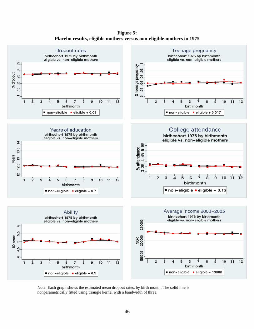
6.4 Placebo results

Table 4 present placebo RD-results for non-eligible mothers in 1977 and eligible mothers

in 1975 where the reform July 1. 1977 is used to test for any effect. We do not find any

significant results for mother’s outcomes in these years. Graphical results comparing

eligible mothers in 1975 to non-eligible mothers in 1975 are presented in Figure 5. We do

not observe any effect from a placebo reform in 1975 in any of the children’s outcomes.

7. Heterogeneous results and mechanisms

We also want to consider how the results may vary across family background. We have a

rich variety of family characteristics like parental education, income, place of residence

and availability of child care at the municipality level. By varying the results by family

background we will also discuss further possible channels through which the maternity

leave may have affected children's outcomes. We will only present results using

differences-in-differences with non-eligible mothers as the control group. The reason is

that by differencing out the month effect we get closer to the causal effect of the reform

since we get closer to satisfy the common trend assumption however we have already

shown in the first set of results that the results are robust to using eligible mothers in 1975

as control group.

- 27 -

7.1 Parental education

We want to see whether maternity leave may have a different effect on mothers with

different educational background and on the children from families with high and low

educated mothers. We split the sample in two; mothers with less than 10 years of

education versus mothers with 10 years or more of education. From Table 5 we see that

children of low educated mothers benefit more from the reform than children with high

educated mothers. This is especially the case when we look at the educational outcomes.

The effect on IQ is approximately the same for both groups, however, the effect on

teenage pregnancy only shows up for the children of more educated parents.30 We see a

stronger effect on mothers probability to return to work within two years after giving

birth when mothers have low education however the effect on the return to work within

five years are similar for the two groups.

7.2 Boys/Girls

We check whether the reform has different impact on boys and girls and also whether

mothers of boys and girls behave differently. Results are presented in Table 6. 31 We see

that the results are more positive and significant for girls than boys. This is supported by

the fact that mothers of girls are also affected slightly more by the reform, especially in

the probability to return to work within two year after giving birth.

30 Using above and below median income for mothers instead of high and low education, provides similar results. 31 Note that the effects we find don IQ earlier is only effects for boys since we have IQ scores only for military service. The effects on teenage pregnancy is only for girls.

- 28 -

7.3 Childcare coverage and proximity to grandparents

As discussed in the section on specification and mechanisms, there are substitutes and

complements to maternal time with children. We have rich data to exploit some of these

possible substitutes and complements. We vary the results by availability of child care in

Table 7.32 We find that the reform had a greater impact on municipalities with low child

care coverage. Typically in Norway you do not send your child to a child care before the

child is one years old. This means that these results may be correlated with the part of the

reform that gives the mother a right to up to one years of unpaid leave in addition to the

paid leave. This is supported by the fact that mothers have a higher probability of

returning to work within two to five years after giving birth when the child care coverage

is low.

Another aspect is the proximity to grandparents. The grandmothers to the children

in our samples would normally not be in the labor force. It was only in the 1960s and

1970s that relatively young women to a large degree entered the labor market. This

means that grandparents may be an available substitute to maternal time with children.

This hinges on the assumption that grandparents live close to their grandchildren so that

they can help out in daily life. We split the sample in two; close means in the same

municipality as your grandparents, while far is further away. We see from the results in

Table 8 that the effect are larger for children when the family live close to grandparents.33

It implies that there does not seem to be a trade-off between mothers staying home with

the child and possibly breast feeding, and grandparents’ time with the child.

32 We have also verified the results by using a polynomial function of birth month and controlled for mothers education, income and age in order to be sure that the results are not driven by differences in mother’s characteristics across municipalities. 33 Again we verified the results by controlling for mothers characteristics.

- 29 -

A reasonable explanation for this could be that grandparents are a weak substitute

to maternal time with the child in the first months of a child life. Before the reform the

mother left the child with her parents while working, but after the reform she stays home

at least for the first four months of the child's life. This support the idea that mother's time

is important in the first months due to breast-feeding and less stress for both mother and

child. A related explanation can be that grandparents are good substitutes to maternal

time later in the child’s life. The results show that mothers living close to her parents

have a greater impact of the reform on the probability to return to work within two to five

years after giving birth. The grandparents can hence constitute a good substitute so that

mother’s can return to their job and increase the resources within a family. Both these

explanations are present in our data and can lead to positive effects on the children’s

outcomes.

7.4 Spillover to other siblings.

Next we present the results of older siblings of the 1977 cohort. If the positive effects on

the outcomes of children affected by the reform also show up in the outcomes of their

older siblings, there are other channels than breastfeeding and intervention in very early

ages that works trough this reform, e.g. mother as a role model.

We define older siblings as those who are 24-48 months34 older than the 1977

cohort.35 Table 9 shows the differences-in-differences results using children of non-

eligible mothers as a control group. We see that the older sibling’s dropout rates are

34 The mean distance between siblings is 35 months. 35 We do not want to include siblings where mother has not finished leave and returned to work before she has the 1977 kid therefore we exclude siblings that are closer than two years in age. The older siblings aged 2-4 is the largest group of siblings, we have also studied siblings older than four; however the sample size is too small to find interesting results.

- 30 -

falling however the effect is not statistically significant. The effect on college attendance

is positive and we see a drop in the probability of teenage pregnancy.36 We do not see any

significant effects on years of schooling or IQ. The reform seems to have some effect on

the older sibling’s outcomes however the effects are much smaller than on the children

directly affected by the reform. We conclude for this result that clearly there are other

mechanisms than through increased breast feeding the extended maternity leave period

worked through.

7.5 Effect of increased income

We next look at the possible effect that it is the increased income through the fact that

there is compensation when taking the extended leave that is important. Table 10 present

parametric polynomial results.37 The first row is the causal effect of the maternity leave

reform on children’s outcomes discussed earlier in Table 3. Then we control for mother’s

income in 1977 to see whether the effect on children changes. We observe that the effects

on children’s outcomes are slightly lower after controlling for income however for most

outcomes, the results are still important and significant. Controlling for all post-reform

characteristics of the mother, income five years after birth, months of leave and return to

work within two to five years after birth does not change the results.

8. Concluding remarks

36 We also perform a placebo tests on older siblings of the 1975 cohort and find no significant effect on any outcomes fro this group. 37 We can not present differences-in-differences here bacuse we want to control for income however our control group, non-eligible mother do not work, hence thay have no income.

- 31 -

Can families, by not working or working less in the first years of a child’s life, influence

the ability of children? And are the potential positive effects large enough to trade-off a

possible negative effect of the parents’ career and earning prospect by taking time off

work with their children? Exploiting a maternity leave reform in Norway, opening up for

up to four months of paid leave and an additional one year of unpaid leave, show us that

this is the case. Children have a higher probability of completing high school, going to

college and have more years of education and boys have a higher IQ score at age 18. By

using yearly income of mothers we have been able to split the sample into eligible and

non-eligible mothers. This has not been done in the literature before and gives us more

precise estimate of the effect of maternity leave on children’s long term outcomes. We

use the rich dataset on family background variables to exploit the effect on mother’s

months of leave, income effects and probability to return to work within two to five years

after giving birth. We find that the reform increases the time mother spend at home with

infants- however they have a higher probability to return to work meaning a better job

protection due to the maternity reform. This support our main source of mechanism of

why an increase in maternity leave should effect children’s outcomes, mother’s spend

more time – quality time – with the child in its first year of life. Then we use the data on

family background to understand more about heterogeneous effects of the reform. We

find that the reform is more effectual for children of low educated mothers.

To understand more the mechanisms driving the results we use measures of

municipality child care coverage and distance to grandparents, and in addition we

measured spillover effects to older under-school age children in the family. The two first

measures may be seen as substitutes (or complements) to maternal time with children.

- 32 -

We find that the reform has more impact on children’s outcomes when the municipality

has low child care coverage and when parents live close to grandparents. The first support

our hypothesis that official child care is a substitute to maternal time, in the long run,

with children while grandparents seem to be complements, in the short run, to maternal

time. When testing effects on older siblings aged 2-4 in 1977, we find some evidence that

the reform also has a positive, although smaller, effect on them indicating that mother’s

behavior as a role model is important. This also suggests a positive spillover effect of the

reform that has to be taken into account when evaluating costs and benefits of introducing

these policies.

For policy implications we conclude that constructing policies to increase parents’

time with children after birth may have an impact on children’s abilities later in life. This

effect has been an important part of the goals behind expansions in maternity leave across

countries; however this study is the first to show that this may also be achieved. There are

not only short terms effects of increasing maternity leave (Tanaka, 2005; Bernal and

Keane, 2006), but also substantial benefits in the long run. As mentioned in the

introduction the situation on maternity leave is remarkably similar in the US today as it

was in Norway before the reform. Parental leave is currently under debate in the US38 and

an introduction of four months of paid leave and better job protection are typically within

feasible policies.39 Using the rich set on family background variables to address

heterogeneity of effects also give us the advantage of making the study less dependent on

institutional settings in Norway. For example by showing that the effects are bigger for

children from lower educated households this may be important for policy discussions

38 USAtoday 26.07.2005, The New York Times 16.04.2008 39 http://www.govtrack.us/congress/bill.xpd?bill=h110-3799

- 33 -

related to lowering inequalities in general. Many countries, like the US, Britain, South

America have a substantial inequality in education and income. While increasing

maternity leave for women and men in these countries will not solve these problems we

have shown that it might reduce the existing gap.

- 34 -

References

American Acadamy of Pediatrics (2005). “Breastfeeding and the Use of Human Milk”,

Pediatrics, 115, 496-506.

Baker, M., and K. S. Milligan (2005). “How Does Job-Protected Maternity Leave Affect

Mothers’ Employment and Infant Health?”, NBER Working Paper Series 11135.

Baker, M., and K. S. Milligan (2008). “Evidence from Maternity Leave Expansion of the

Impact of Maternal Care on Early Child Development”, NBER Working Paper

Series 13826.

Baum, C. L. (2003). “Does Early Maternal Employment Harm Child Development? An

Analysis of the Potential Benefits of Leave Taking”, Journal of Labor Economics,

21, 609-448.

Becker, G. and N. Tomes (1986). “Human Capital and the Rise and Fall of Families”,

Journal of Labor Economics, 4, 1-39.

Berger, L. M., J. Hill, and J. Waldfogel (2005). “Maternity Leave, Early Maternal

Employment and Child Health and Development in the US”, The Economic

Journal, 115, 29-47.

Bernal, R., and J. M. Keane (2006). “The Effect of Maternal Employment and Child Care

on Children’s Cognitive Development”, Northwestern University, mimeo

Black, S., P. Devereux, and K. G. Salvanes (2005). “The More the Merrier? The Effect of

Family Size and Birth Order on Children’s Education”, Quarterly Journal of

Economics, 120, 667-700.

Black, S., P. Devereux, and K. G. Salvanes (2008). “Too Young to Leave the Nest?

The Effects of School Starting Age” NBER working paper No. 13969.

Blau, D. M. and A. P. Hagy (1998): The Demand for Quality in Child Care.

Journal of Political Economy, 106, 104-145

Card, D. and D. Le (2008). “Regression Discontinuity Inference with Specification”

Journal of Econometrics, 142, 655-674

Carneiro, P., and J. Heckman (2003). “Human Capital Policies”, in J. Heckman, A.

Krueger (Eds.), Inequality in America: What Role for Human Capital Policies.

MIT Press.

- 35 -

Concato, J. A. and J.M. Leventhal (2002). “How Good is the Evidence Linking

Breastfeeding and Intelligence?” Pediatrics, 109(6), 1044-53.

Dustmann, C., and U. Schønberg (2007). 2The Effect of Expansions in Maternity Leave

Coverage on Children’s Long-Term Outcomes”, European Society of Population

Economics Conference, Chicago. mimeo.

Hahn, J., P. Todd, and W. Van der Klauw (2001). ”Identifcation and Estimation of

Treatment Effects with a Regression-Discontinuity Design”, Econometrica, 69,

201-209.

Han, W., C. Ruhm, and J. Waldfogel (2007). “Parental Leave Policies and Parents’

Employment and Leave-Taking”, NBER Working Paper Series 13697.

Heckman, J. (2006). “Skill Formation and the Economics of Investing in Disadvantaged

Children”, Science, 312, 1900-1902.

Heckman, J. and D. Masterov (2007). 2The Productivity Argument for Investing in

Young Children”, NBER Working Paper Series 13016.

Hill, J., J. Waldfogel, J. Brooks-Gunn, and W. Han (2005). “Maternal Employment and

Child Development: A Fresh Look Using Newer Methods”, Developmental

Psychology, 41, 833-850.

Imbens, G. W. and T. Lemieux (2008). “Regression Discontinuity Designs: A Guide to

Practice”. Journal of Econometrics, 142, 615-635.

Ip, S. M. Chung, G. Raman, P. Chew, N. Magula, D. DeVine, T. Trikalinos, and L. Lau

(2007). “Breastfeeding and Maternal and Infamt Outcomes in Developed

Countries.” Evidence Report/Technology Assessment No. 153, Agency for

Healthcare Research and Quality, 1-196.

Kramer, M.S. and R. Kakuma (2004). “The Optimal Duration of Exclusive

Breastfeeding: A Systematic Review” Advances in Experimental Medicine and

Biology, 554, 65-77.

Lalive, R., and J. Zweimuller (2005). “Does Parental Leave Affect Fertility and Return

to-Work? Evidence from a "True Natural Experiment", IZA Discussion Paper

1613.

Liestøl, K., M. Rosenberg, and L. Walløe (1988).”Breastfeeding Practice in Norway

1860-1984.” Journal of Biosocial Science, 20, 45-58.

- 36 -

Ludsteck, J., and U. Schønberg (2007). “Maternity Leave Legislation, Female Labor

Supply and the Family Wage Gap”, mimeo.

Ludwig, J and D. Miller (2007). “Does Head Start Improve Children’s Life Chances?

Evidence from a Regression Discontinuity Design”. The Quarterly Journal of

Economics, 122, 159-208.

Mortensen, E.L, K.F. Michaelsen, S.A. Sanders and J.M. Reinich (2002). “The

Association Between Duration of Breatfeeding and Adult Intelligence” Journal of

the American Medical Association, 287(19), 2365-71.

Porter, J (2003). “Estimation in the Regression Discontinuity Design”, mimeo, University

of Wisconsin.

Ramey, C. T., and S. L. Ramey (1998). “Early Intervention and Early Experience”,

American Psychologist, 53, 109-120.

Ruhm, C. J. (2000). “Parental Leave and Child Health”, Journal of Health Economics,

19, 931-960.

Ruhm, C. J. (2004): Parental Employment and Child Cognitive Development.,

Journal of Human Resources, 39, 155-192.

Rønsen, M. and M. Sundstrøm (2002). “Family Policy and After-Birth Employment

Among New Mothers – A Comparison of Finland, Norway and Sweden”, European

Journal of Population, 18, 121-152

Tanaka, S. (2005). “Parental Leave and Child Health Across OECD Countries”, The

Economic Journal, 115, 7-28.

Waldfogel, J. (2007). “Welfare Reforms and Child Well-Being in the US and UK”

CASE-paper, mimeo.

Wurtz, A. (2007). “The Long-Term Effect on Children of Increasing the Length of

Parents. Birth-Related Leave”, Aarhus School of Business, Department of

Economics Working Paper 07-11.

- 37 -

Figure 1

Parental leave reforms in Norway

0 10 20 30 40 50 60

Weeks

195601.07.197701.05.1987

01.07.198801.04.1989

01.05.199001.07.199101.04.1992

01.04.1993

Parental leave reforms

unpaid leavePaid leave

Source: regjeringen.no, lovdata.no

- 38 -

39

Figure 2 Mother’s characteristics by birth month, eligible mothers 1977

Note: Each graph shows the estimated mean characteristic for mothers birth month. The solid line is nonparametrically fitted using triangle kernel with a bandwidth of three.

40

Figure 3a Mother’s outcomes by birth month, eligible mothers 1977

Note: Each graph shows the estimated mean for mother’s outcomes by birth month. The solid line is non-parametrically fitted using triangle kernel with a bandwidth of three.

41

Figure 3b Mother’s outcomes by birth month, eligible mothers 1977 versus non-eligible

mothers 1977 and eligible mothers 1975

Note: Each graph shows the estimated mean for mother’s outcomes by birth month. The solid line is non-parametrically fitted using triangle kernel with a bandwidth of three.

42

Figure 4a Children’s outcomes by birth month, eligible mothers 1977

Note: Each graph shows the estimated mean characteristic for children’s outcomes, by birth month. The solid line is nonparametrically fitted using triangle kernel with a bandwidth of three.

43

Figure 4b Children’s outcomes by birth month, eligible mothers 1977 versus non-eligible


Note: Each graph shows the estimated mean dropout rates, by birth month. The solid line is nonparametrically fitted using triangle kernel with a bandwidth of three.

44

Figure 4c Children’s outcomes by birth month, eligible mothers 1977 versus non-eligible


Note: Each graph shows the estimated mean dropout rates, by birth month. The solid line is nonparametrically fitted using triangle kernel with a bandwidth of three

45

Figure 4d Children’s outcomes by birth month, eligible mothers 1977 versus non-eligible



46

Figure 5: Placebo results, eligible mothers versus non-eligible mothers in 1975


47

Table 1 Descriptive statistics, eligible mothers and children of eligible mothers in 1977

Birth month January - June

July - December Difference

Mothers

Years of education 10.71 (.019)

10.70 (.020)

-.006 (.028)

Age at birth (in months)

314.44 (.481)

315.15 (.515)

.707 (.704)

Income in 1975 in NOK

103,868 (573)

97,105 (628)

-6,764*** (849)


69,922 (573)

10,4810 (611)

34,888*** (837)


75,496 (642)

74,586 (679)

-910 (934)

Predicted months of leave 4.157 (.040)

6.309 (.018)

2.15*** (.045)

Probability to return to work within 2 years

.751 (.004)

.750 (.004)

-.001 (.005)

Probability to return to work within 5 years

.772 (.004)

.769 (.004)

-.004 (.005)

Children

Dropout rates .181 (.003)

.172 (.003)

-.009** (.005)

College attendance

.479 (.004)

.476 (.005)

-.003 (.006)

Years of education

13.06 (.021)

13.02 (.022)

-.035 (.030)

Teenage pregnancy

.021 (.001)

.019 (.001)

-.002* (.001)

IQ young men

5.425 (.022)

5.413 (.024)

-.012 (.032)

Average income 2003-2005

in NOK

206,446 (977)

204,879 (1027)

-1567 (1417)

Note: 1USD=5.23NOK (16.06.2008)

48

Table 2a The effects of maternity leave reform on mother’s labor supply

Regression Discontinuity

Variables

Mean

Nonparametric

Parametric Quadratic

Parametric 4th order

poly. Bandwidth 2 3 4 3 6

Predicted months of leave

5.2 2.204***

(.078) 2.207***

(.071) 2.198***

(.065) 2.230***

(.054) 2.317***

(.056)

Ln(Income) (1977)

10.98 .242***

(0.036) .244*** (0.029)

.241*** (.028)

.181*** (0.006)

.168*** (.017)

Return 2 years after birth

.75 .022*

(.014) .026** (.012)

.024** (.011)

.038*** (.006)

.023*** (.008)


.77 .028**

(.014) .026** (.010)

.024** (.011)

.033*** (0.005)

.026*** (.007)

Ln(Income) 5 years after birth

11.02 .028

(0.050) .025

(.041) .009

(.037) .041

(.049) -.008 (.045)

Each cell presents the estimated discontinuity in the outcomes as a result of the maternity leave reform July 1st 1977. We estimate regressions using local linear regression as in Hahn et al. (2003) and derive analytic standard errors based on formulas in Porter (2003) using a triangle kernel. We also present parametric results using a 2nd order and a 4th order polynomial function of birth month. We cluster standard errors as in Lee and Card (2007). ***significant at 1 %, **significant at 5%, *significant at 10%, N=25645

49

Table 2b The effects of maternity leave reform on mother’s labor supply

Differences-in-differences using non-eligible mothers 1977 and eligible mothers 1975

Variables

Nonparametric difference-in-differences estimates

Bandwidth 2 3 4

Control group

Noneligible 1977

Eligible 1975

Noneligible 1977

Eligible 1975

Noneligible 1977

Eligible 1975


.028** (.012)

.008 (.010)

.031*** (.010)

.014* (.009)

.029*** (.009)

.010 (.008)


.036*** (.011)

.025** (.010)

.038*** (.010)

.026*** (.008)

.036*** (.009)

.026*** (.008)

Each cell presents the estimated discontinuity in the outcomes as a result of the maternity leave reform July 1st 1977. We estimate regressions using local linear regression as in Hahn et al. (2003) and derive analytic standard errors based on formulas in Porter (2003) using a triangle kernel. We also present parametric results using a 2nd order and a 4th order polynomial function of birth month. We cluster standard errors as in Lee and Card (2007) under the assumption that that the trend in outcomes would be the same before and after the reform. ***significant at 1 %, **significant at 5%, *significant at 10%, N=48515 (eligible 1977 and non-eligible 1977), N=50716 (eligible 1977 and eligible 1975)

50

Table 3a The effects of maternity leave reform on children’s outcomes

Regression Discontinuity

Variables

Mean

Nonparametric


Parametric 4th order

poly. Bandwidth 2 3 4 3 6

Dropout rate

.18 -.026**

(.012) -.025** (.011)

-.020** (.010)

-.033*** (.008)

-.025*** (.009)

College attendance

.47 .024

(.016) .025* (.014)

.018 (.013)

.041*** (.006)

.024* (.012)

Years of schooling

13.04 .140*

(.080) .133* (.068)

.095 (.06)

.198*** (.037)

.106 (.069)

Teenage pregnancy

.025 -.003

(.005) -.003 (.004)

-.003 (.004)

-.002 (.001)

-.004 (.004)

IQ (boys)

5.42 .142*

(.082) .110

(.072) .078

(.064) .155** (0.057)

.099 (0.084)

Ln(Income) 2003-2005

12.09 .017

(.030) .024

(.021) .022

(.021) .043*** (0.012)

.030*** (0.009)

Each cell presents the estimated discontinuity in the outcomes as a result of the maternity leave reform July 1st 1977. We estimate regressions using local linear regression as in Hahn et al. (2003) and derive analytic standard errors based on formulas in Porter (2003) using a triangle kernel. We also present standard errors and p-values derived from bootstrapping using 1000 replications. We also present parametric results using a 2nd order and a 4th order polynomial function of birth month. We cluster standard errors as in Lee and Card (2007). ***significant at 1 %, **significant at 5%, *significant at 10%, N=25645

51

Table 3b The effects of maternity leave reform on children’s outcomes

Differences-in-differences using non-eligible mothers 1977 and eligible mothers 1975

Variables


Bandwidth 2 3 4

Control group

Non-elig. 1977

Eligible 1975

Non-elig. 1977

Eligible 1975

Non-elig. 1977

Eligible 1975

Dropout rate

-.025** (.010)

-.029*** (.009)

-.024*** (.009)

-.031*** (.008)

-.021*** (.008)

-.028*** (.007)

College attendance

.022** (.012)

.039*** (.011)

.023** (.010)

.044*** (.010)

.019** (.009)

.039*** (.009)

Years of schooling

.143** (.059)

.174*** (.057)

.153*** (.050)

.196*** (.049)

.130*** (.046)

.175*** (.044)

Teenage pregnancy

-.012*** (.004)

-.005* (.003)

-.010*** (.004)

-.005* (.003)

-.010*** (.003)

-.005* (.003)

IQ (boys)

.149** (.063)

.232*** (.059)

.158*** (.054)

.189*** (.051)

132*** (.049)

.140*** (.046)


.014 (.021)

.027 (.020)

.021 (.016)

.030** (.014)

.022 (.016)

.024* (.014)

Each cell presents the estimated discontinuity in the outcomes as a result of the maternity leave reform July 1st 1977. We estimate regressions using local linear regression as in Hahn et al. (2003) and derive analytic standard errors based on formulas in Porter (2003) using a triangle kernel. We also present parametric results using a 2nd order and a 4th order polynomial function of birth month. We cluster standard errors as in Lee and Card (2007) under the assumption that that the trend in outcomes would be the same before and after the reform. ***significant at 1 %, **significant at 5%, *significant at 10%, N=48515 (eligible 1977 and non-eligible 1977), N=50716 (eligible 1977 and eligible 1975)

52

Table 4 Placebo results: The effects of maternity leave reform on mother’s labor supply and

children’s outcomes Non-eligible mothers 1977 and eligible mothers 1975

Variables

Nonparametric

Bandwidth 2 3 4 Control group

Non-elig. 1977

Eligible 1975

Non-elig. 1977

Eligible 1975

Non-elig. 1977

Eligible 1975

Dropout rate

.008 (.013)

-.001 (.015)

.007 (.011)

-.001 (.013)

.008 (.010)

.002 (.012)

College attendance

-.015 (.016)

.002 (.017)

-.020 (.014)

.002 (.014)

-.018 (.013)

-.001 (.013)

Years of schooling

-.034 (.082)

-.003 (.083)

-.064 (.070)

-.020 (.071)

-.080 (.064)

-.035 (.064)

Teenage pregnancy

.004 (.005)

.004 (.008)

.004 (.005)

.004 (.007)

.003 (.004)

.005 (.006)

IQ (boys)

-.089 (.083)

-.006 (.090)

-.078 (.072)

-.048 (.078)

-.061 (.065)

-.054 (.070)


-.010 (.027)

.003 (.031)

-.006 (.019)

.003 (.023)

-.002 (.020)

.000 (.022)

Ln(Income) (1977)

- - -

- -

-


.015 (.015)

-.005 (.017)

.012 (.013)

-.006 (.015)

.014 (.012)

-.006 (.013)


.002 (.014)

-.008 (.017)

-.000 (.012)

-.012 (.015)

-.003 (.011)

-.013 (.013)


-.002 (0.050)

- .016

(.042)

- .022

(.039)

-

Each cell presents the estimated discontinuity in the outcomes as a result of the maternity leave reform July 1st 1977. We estimate regressions using local linear regression as in Hahn et al. (2003) and derive analytic standard errors based on formulas in Porter (2003) using a triangle kernel. We also present parametric results using a 4th order polynomial function of birth month. We cluster standard errors as in Lee and Card (2007). ***significant at 1 %, **significant at 5%, *significant at 10%, N=22869 (eligible 1977 and non-eligible 1977), N=25071 (eligible 1977 and eligible 1975)

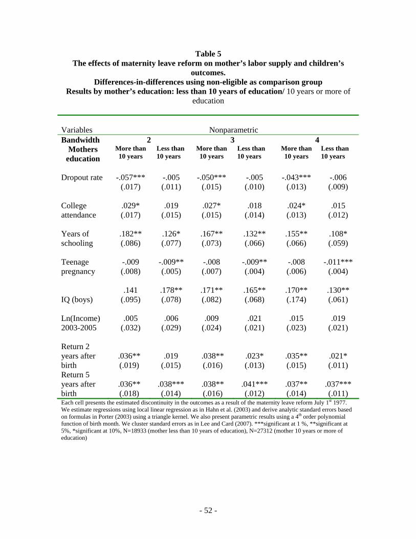
- 52 -

Table 5 The effects of maternity leave reform on mother’s labor supply and children’s

outcomes. Differences-in-differences using non-eligible as comparison group

Results by mother’s education: less than 10 years of education/ 10 years or more of education

Variables

Nonparametric

Bandwidth 2 3 4 Mothers

education More than 10 years

Less than 10 years

More than 10 years

Less than 10 years

More than 10 years

Less than 10 years

Dropout rate

-.057***

(.017)

-.005 (.011)

-.050***

(.015)

-.005 (.010)

-.043***

(.013)

-.006 (.009)

College attendance

.029* (.017)

.019

(.015)

.027* (.015)

.018

(.014)

.024* (.013)

.015

(.012) Years of schooling

.182** (.086)

.126* (.077)

.167** (.073)

.132** (.066)

.155** (.066)

.108* (.059)

Teenage pregnancy

-.009 (.008)

-.009** (.005)

-.008 (.007)

-.009** (.004)

-.008 (.006)

-.011***

(.004) IQ (boys)

.141

(.095)

.178** (.078)

.171** (.082)

.165** (.068)

.170** (.174)

.130** (.061)


.005

(.032)

.006

(.029)

.009

(.024)

.021

(.021)

.015

(.023)

.019

(.021)


.036** (.019)

.019

(.015)

.038** (.016)

.023* (.013)

.035** (.015)

.021* (.011)


.036** (.018)

.038*** (.014)

.038** (.016)

.041*** (.012)

.037** (.014)

.037*** (.011)

Each cell presents the estimated discontinuity in the outcomes as a result of the maternity leave reform July 1st 1977. We estimate regressions using local linear regression as in Hahn et al. (2003) and derive analytic standard errors based on formulas in Porter (2003) using a triangle kernel. We also present parametric results using a 4th order polynomial function of birth month. We cluster standard errors as in Lee and Card (2007). ***significant at 1 %, **significant at 5%, *significant at 10%, N=18933 (mother less than 10 years of education), N=27312 (mother 10 years or more of education)

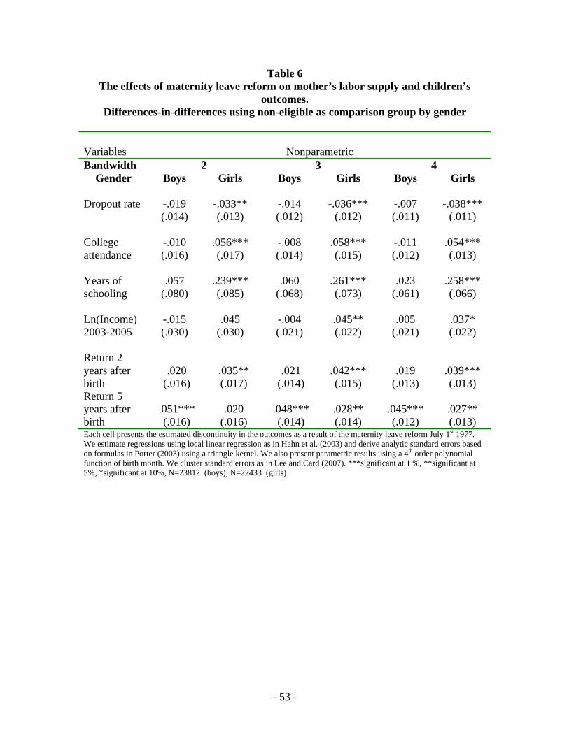
- 53 -


outcomes. Differences-in-differences using non-eligible as comparison group by gender

Variables

Nonparametric

Bandwidth 2 3 4 Gender Boys Girls Boys Girls Boys Girls

Dropout rate

-.019 (.014)

-.033** (.013)

-.014 (.012)

-.036***

(.012)

-.007 (.011)

-.038***

(.011) College attendance

-.010 (.016)

.056*** (.017)

-.008 (.014)

.058*** (.015)

-.011 (.012)

.054*** (.013)

Years of schooling

.057

(.080)

.239*** (.085)

.060

(.068)

.261*** (.073)

.023

(.061)

.258*** (.066)


-.015 (.030)

.045

(.030)

-.004 (.021)

.045** (.022)

.005

(.021)

.037* (.022)


.020

(.016)

.035** (.017)

.021

(.014)

.042*** (.015)

.019

(.013)

.039*** (.013)


.051*** (.016)

.020

(.016)

.048*** (.014)

.028** (.014)

.045*** (.012)

.027** (.013)

Each cell presents the estimated discontinuity in the outcomes as a result of the maternity leave reform July 1st 1977. We estimate regressions using local linear regression as in Hahn et al. (2003) and derive analytic standard errors based on formulas in Porter (2003) using a triangle kernel. We also present parametric results using a 4th order polynomial function of birth month. We cluster standard errors as in Lee and Card (2007). ***significant at 1 %, **significant at 5%, *significant at 10%, N=23812 (boys), N=22433 (girls)

- 54 -



Results by child care coverage.

Variables

Nonparametric

Bandwidth 2 3 4 Child care coverage

low high low high low high

Dropout rate

-.054***

(.014)

.003

(.014)

-.059***

(.012)

.008

(.012)

-.064***

(.011)

.018


.040** (.017)

.004

(.016)

.042*** (.015)

.006

(.014)

.042*** (.013)

-.002 (.013)

Years of schooling

.224*** (.082)

.057

(.083)

.268*** (.071)

.043

(.071)

.286*** (.064)

-.014 (.064)

Teenage pregnancy

-.012* (.006)

-.010* (.006)

-.011** (.006)

-.008 (.005)

-.011** (.005)

-.007* (.005)

IQ (boys)

.116

(.089)

.207** (.087)

.123* (.077)

.216*** (.075)

.126* (.070)

.163** (.068)


.004

(.030)

.025

(.030)

.011

(.022)

.034

(.022)

.017

(.022)

.030

(.022)


.036** (.017)

.021

(.016)

.039*** (.015)

.025* (.014)

.034*** (.013)

.026** (.013)


.043*** (.016)

.028* (.015)

.050*** (.014)

.027** (.013)

.049*** (.013)

.024** (.012)

Each cell presents the estimated discontinuity in the outcomes as a result of the maternity leave reform July 1st 1977. We estimate regressions using local linear regression as in Hahn et al. (2003) and derive analytic standard errors based on formulas in Porter (2003) using a triangle kernel. We also present parametric results using a 4th order polynomial function of birth month. We cluster standard errors as in Lee and Card (2007). ***significant at 1 %, **significant at 5%, *significant at 10%, N=22305 (low child care coverage), N=23940 (high child care coverage)

- 55 -



Results by distance to grandparents

Variables

Nonparametric

Bandwidth 2 3 4 Distance to

grandparents Close Not-close Close Not-close Close Not-clsoe

Dropout rate

-.067***

(.019)

-.012 (.013)

-.069***

(.017)

-.010 (.012)

-.078***

(.015)

-.006 (.010)

College attendance

.110*** (.023)

-.026* (.016)

.099*** (.020)

-.022 (.014)

.089*** (.018)

-.021* (.012)

Years of schooling

.476*** (.113)

-.037 (.079)

.488*** (.097)

-.041 (.067)

.482*** (.088)

-.053 (.061)

Teenage pregnancy

-.007 (.009)

-.008 (.006)

-.006 (.008)

-.006 (.005)

-.008 (.007)

-.006 (.005)

IQ (boys)

.588*** (.123)

-.018 (.084)

.569*** (.108)

.013

(.072)

.441*** (.096)

.031

(.065) Ln(Income) 2003-2005

.109** (.043)

-.037 (.028)

.109*** (.031)

-.032 (.021)

.095*** (.030)

-.024 (.021)


.072*** (.024)

.025

(.016)

.066*** (.021)

.032** (.014)

.063*** (.019)

.031*** (.012)


.068*** (.023)

.024

(.015)

.071*** (.020)

.027** (.013)

.065*** (.018)

.025** (.012)

Each cell presents the estimated discontinuity in the outcomes as a result of the maternity leave reform July 1st 1977. We estimate regressions using local linear regression as in Hahn et al. (2003) and derive analytic standard errors based on formulas in Porter (2003) using a triangle kernel. We also present parametric results using a 4th order polynomial function of birth month. We cluster standard errors as in Lee and Card (2007). ***significant at 1 %, **significant at 5%, *significant at 10%, N=11405 (close to grandparents), N=25857 (far from grandparents)

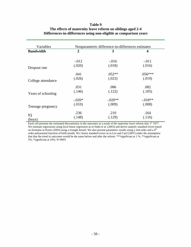
- 56 -

Table 9 The effects of maternity leave reform on siblings aged 2-4

Differences-in-differences using non-eligible as comparison years

Variables


Bandwidth 2 3 4 Dropout rate

-.012 (.020)

-.016 (.018)

-.011 (.016)

College attendance

.041 (.026)

.052** (.023)

.056*** (.019)

Years of schooling

.031 (.146)

.086 (.122)

.082 (.105)

Teenage pregnancy

-.020* (.010)

-.020** (.009)

-.018** (.008)

IQ (boys)

.236 (.148)

.210 (.129)

.164 (.116)

Each cell presents the estimated discontinuity in the outcomes as a result of the maternity leave reform July 1st 1977. We estimate regressions using local linear regression as in Hahn et al. (2003) and derive analytic standard errors based on formulas in Porter (2003) using a triangle kernel. We also present parametric results using a 2nd order and a 4th order polynomial function of birth month. We cluster standard errors as in Lee and Card (2007) under the assumption that that the trend in outcomes would be the same before and after the reform. ***significant at 1 %, **significant at 5%, *significant at 10%, N=9693

- 57 -

Table 10 The effects of maternity leave reform on children’s outcomes

Using 2nd and 4th order polynomial Control for mothers post-reform characteristics

Variables


Parametric 4th order poly.

Bandwidth 3 6

Dropout rate

-.033***

(.008)

-.026***

(.005)

-.028***

(.005)

-.025***

(.009)

-.020***

(.007)

-.022***


.041*** (.006)

.024*** (.003)

.030*** (.001)

.024* (.012)

.011

(.008)

.016* (.009)

Years of schooling

.198*** (.037)

.136*** (.020)

.151*** (.030)

.106

(.069)

.059

(.053)

.077

(.058) Teenage pregnancy

-.002 (.001)

.000

(.001)

.004

(.002)

-.004 (.004)

-.003 (.003)

.002

(.004) IQ (boys)

.155** (.057)

.101** (.033)

.102** (.040)

.099

(.084)

.045

(.063)

.047

(.066) Ln(Income) 2003-2005

.043*** (.012)

.043*** (.012)

.045*** (.014)

.030*** (.009)

.028** (.010)

.027** (.009)

Controls No Only mothers

income in 1977

All mothers post-reform outcomes

No Only mothers

income in 1977

All mothers

post- reform

outcomes We present parametric results using a 2nd order and a 4th order polynomial function of birth month. We cluster standard errors as in Lee and Card (2007). ***significant at 1 %, **significant at 5%, *significant at 10%

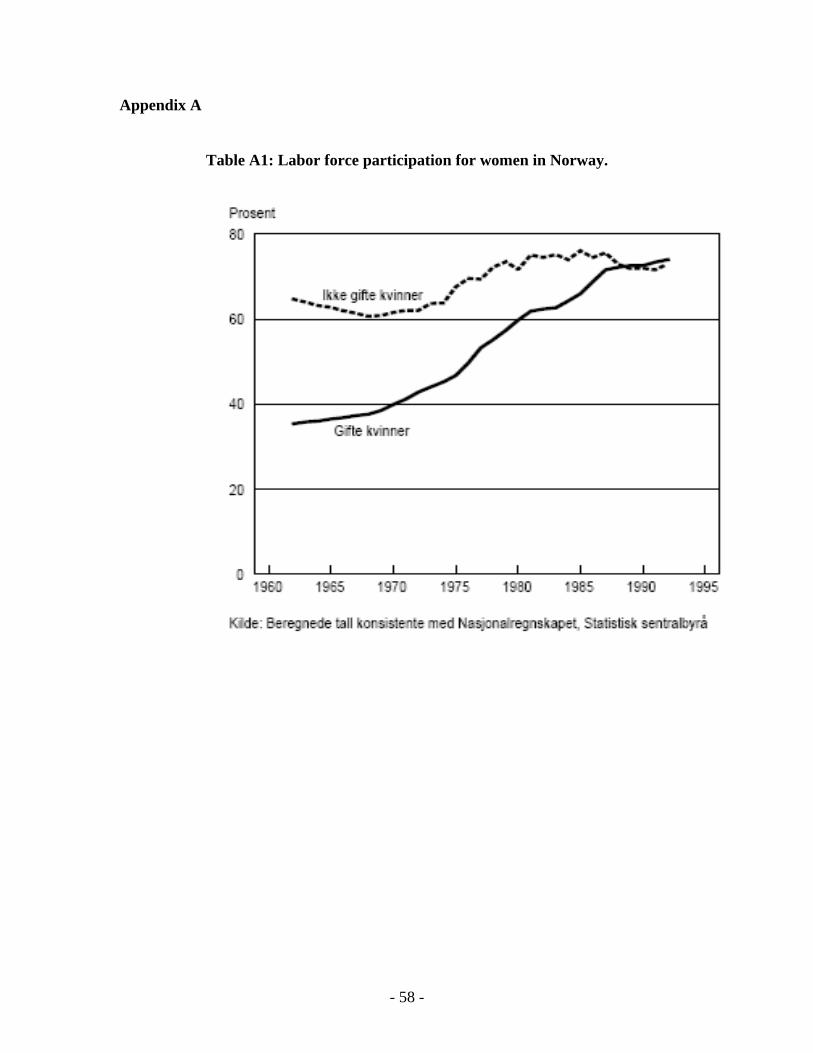
- 58 -

Appendix A

Table A1: Labor force participation for women in Norway.

- 59 -

Table A2 The effects of maternity leave reform on mother’s labor supply and children’s outcomes using the total sample of all mothers and children in 1977 and 1975 RD results all mothers in 1977/Diff-in-diff using all mothers in 1975 and 1977

Variables

Nonparametric RD and difference-in-differences estimates

Bandwidth 2 3 4

Dropout rate

-.015 (.010)

-.014** (.007)

-.013 (.009)

-.012** (.006)

-.009 (.008)

-.010* (.005)

College attendance

.009 (.012)

.013 (.008)

.009 (.010)

.016** (.007)

.004 (.009)

.014** (.006)

Years of schooling

.054 (.059)

.050 (.041)

.035 (.050)

.047 (.035)

.003 (.046)

.033 (.032)

Teenage pregnancy

.002 (.004)

.002 (.003)

.002 (.004)

.002 (.003)

.002 (.003)

.002 (.003)

IQ (boys)

.060 (.062)

.128*** (.043)

027 (.054)

.086** (.037)

.006 (.049)

.046 (.034)


.012 (.021)

.019 (.014)

.015 (.016)

.019* (.010)

.012 (.015)

.012 (.010)


-.007 (.012)

-.011 (.008)

-.006 (.010)

-.010 (.007)

-.008 (.009)

-.010 (.006)


-.002 (.011)

-.008 (.008)

-.005 (.010)

-.009 (.007)

-.007 (.009)

-.007 (.006)


-.001 (.042) - -.006

(.035) - -.015 (.032) -

Each cell presents the estimated discontinuity in the outcomes as a result of the maternity leave reform July 1st 1977. We estimate regression x using local linear regression as in Hahn et al. (2003) and derive analytic standard errors based

on formulas in Porter (2003) using a triangle kernel. We also present standard errors and p-values derived from bootstrapping using 1000 replications. We also present parametric results using a 2nd order and a 4th order polynomial function of birth month. We cluster standard errors as in Lee and Card (2007). ***significant at 1 %, **significant at

5%, *significant at 10%, N=46245 (RD), N=97312 (diff-in-diff using 1975 as control group)

A flying start? Maternity leave and long-term outcomes for ... · A flying start? Maternity leave and long-term ... child an advantage also later in adult school ... was supposed

Documents