A Flight Dynamics Model for a Multi-Actuated Flexible Rocket Vehicle Jeb S. Orr * Science Applications International Corporation, Huntsville, AL 35806, USA A comprehensive set of motion equations for a multi-actuated flight vehicle is presented. The dynamics are derived from a vector approach that generalizes the classical linear perturbation equations for flexible launch vehicles into a coupled three-dimensional model. The effects of nozzle and aerosurface inertial coupling, sloshing propellant, and elasticity are incorporated without restrictions on the position, orientation, or number of model elements. The present formulation is well suited to matrix implementation for large-scale linear stability and sensitivity analysis and is also shown to be extensible to nonlinear time-domain simulation through the application of a special form of Lagrange’s equations in quasi-coordinates. The model is validated through frequency-domain response comparison with a high-fidelity planar implementation. I. Introduction Modeling the behavior of a flexible booster in atmospheric flight is a non-trivial exercise in dynamics that has been treated with various levels of fidelity over the last fifty years by practitioners of the art. For the purposes of basic sizing and performance analysis, it is often sufficient to assume the vehicle is a rigid body or even a point mass and propagate the trajectory considering as few as two degrees of freedom. Traditionally, physical vehicle and trajectory design considerations have helped to ensure that the simulated behavior was closely replicated in the actual system; for example, great expense is incurred in eliminating nonlinearity from the physical system so as to ensure that the flight control stability problem is tractable using classical linear techniques. Despite the intentional design simplifications, simulation and analysis of this class of flight vehicle requires a carefully constructed and well-understood dynamics model that considers the significant coupling effects between the rigid body dynamics, structural modes, sloshing propellant, aerodynamics, servodynamics, and the flight control system. Control-structure interaction is often the chief design challenge, especially in boosters with large slenderness ratio and low structural mass. In an era of emerging unconventional approaches to the design of launch vehicles, missiles, and hypersonic aircraft, traditional (namely, planar) dynamics models 1,2 may no longer be sufficient for modeling the vehicle dynamics for the purposes of stability analysis and control design. Traditionally, by virtue of a set of body axes generally aligned with the principle moments of inertia, it could be assumed that the control system axes were fundamentally decoupled. Clearly, this is not possible in the more general case, and more importantly, the structural response may have a strong multi-axis character. Finally, multi-actuation is not well-treated by traditional models, which may assume a set of identically performing, non-interacting actuators and nozzle masses that are lumped together in order to compute inertial coupling effects. 1 The intent of the present formulation is to overcome these and other restrictions in fidelity and scalability while retaining the general character of the linear perturbation models from which this new approach originates. Indeed, the present formulation is derived using almost the same technique as in the planar case, albeit much more rigorously owing to the matrix-vector nature of the mechanics. Ultimately, the result is a compact recipe for modeling flexible aerospace systems with multiple attached effectors, including provisions for sloshing propellant. With parameters fixed in time, the equations of motion are readily implemented in linear form so as to generate a linear state-space model for control design. If the nonlinear terms are included, the formulation can be integrated numerically as a high-fidelity mechanization of the full vehicle dynamics. Thus, the application of the model is twofold: rather than propagate a nonlinear trajectory simulation and load the resultant parameters into an analytic stability model (or numerically linearize a nonlinear simulation), the nonlinear equations of motion can be directly linearized at certain operating points for analysis. The present formulation is known as an integrated formulation, which differs from a multi-body formulation. In a multi-body formulation, the equations of motion for each body are written with respect to an inertial frame, and the necessary interbody forces are solved as a set of adjoint or constraint equations that relate the motion of each * Flight Controls Engineer, Space Engineering Technology Division 1 American Institute of Aeronautics and Astronautics https://ntrs.nasa.gov/search.jsp?R=20110015712 2018-06-18T15:29:05+00:00Z

Welcome message from author
This document is posted to help you gain knowledge. Please leave a comment to let me know what you think about it! Share it to your friends and learn new things together.
Transcript
A Flight Dynamics Model for a Multi-Actuated FlexibleRocket Vehicle
Jeb S. Orr∗
Science Applications International Corporation, Huntsville, AL 35806, USA
A comprehensive set of motion equations for a multi-actuated flight vehicle is presented. The dynamicsare derived from a vector approach that generalizes the classical linear perturbation equations for flexiblelaunch vehicles into a coupled three-dimensional model. The effects of nozzle and aerosurface inertial coupling,sloshing propellant, and elasticity are incorporated without restrictions on the position, orientation, or numberof model elements. The present formulation is well suited to matrix implementation for large-scale linearstability and sensitivity analysis and is also shown to be extensible to nonlinear time-domain simulation throughthe application of a special form of Lagrange’s equations in quasi-coordinates. The model is validated throughfrequency-domain response comparison with a high-fidelity planar implementation.
I. Introduction
Modeling the behavior of a flexible booster in atmospheric flight is a non-trivial exercise in dynamics that has beentreated with various levels of fidelity over the last fifty years by practitioners of the art. For the purposes of basicsizing and performance analysis, it is often sufficient to assume the vehicle is a rigid body or even a point mass andpropagate the trajectory considering as few as two degrees of freedom. Traditionally, physical vehicle and trajectorydesign considerations have helped to ensure that the simulated behavior was closely replicated in the actual system;for example, great expense is incurred in eliminating nonlinearity from the physical system so as to ensure that theflight control stability problem is tractable using classical linear techniques.
Despite the intentional design simplifications, simulation and analysis of this class of flight vehicle requires acarefully constructed and well-understood dynamics model that considers the significant coupling effects betweenthe rigid body dynamics, structural modes, sloshing propellant, aerodynamics, servodynamics, and the flight controlsystem. Control-structure interaction is often the chief design challenge, especially in boosters with large slendernessratio and low structural mass.
In an era of emerging unconventional approaches to the design of launch vehicles, missiles, and hypersonic aircraft,traditional (namely, planar) dynamics models1,2 may no longer be sufficient for modeling the vehicle dynamics for thepurposes of stability analysis and control design. Traditionally, by virtue of a set of body axes generally aligned withthe principle moments of inertia, it could be assumed that the control system axes were fundamentally decoupled.Clearly, this is not possible in the more general case, and more importantly, the structural response may have a strongmulti-axis character. Finally, multi-actuation is not well-treated by traditional models, which may assume a set ofidentically performing, non-interacting actuators and nozzle masses that are lumped together in order to computeinertial coupling effects.1
The intent of the present formulation is to overcome these and other restrictions in fidelity and scalability whileretaining the general character of the linear perturbation models from which this new approach originates. Indeed,the present formulation is derived using almost the same technique as in the planar case, albeit much more rigorouslyowing to the matrix-vector nature of the mechanics. Ultimately, the result is a compact recipe for modeling flexibleaerospace systems with multiple attached effectors, including provisions for sloshing propellant. With parameters fixedin time, the equations of motion are readily implemented in linear form so as to generate a linear state-space modelfor control design. If the nonlinear terms are included, the formulation can be integrated numerically as a high-fidelitymechanization of the full vehicle dynamics. Thus, the application of the model is twofold: rather than propagatea nonlinear trajectory simulation and load the resultant parameters into an analytic stability model (or numericallylinearize a nonlinear simulation), the nonlinear equations of motion can be directly linearized at certain operatingpoints for analysis.
The present formulation is known as an integrated formulation, which differs from a multi-body formulation. Ina multi-body formulation, the equations of motion for each body are written with respect to an inertial frame, andthe necessary interbody forces are solved as a set of adjoint or constraint equations that relate the motion of each∗Flight Controls Engineer, Space Engineering Technology Division
1American Institute of Aeronautics and Astronautics
https://ntrs.nasa.gov/search.jsp?R=20110015712 2018-06-18T15:29:05+00:00Z
body to its adjacent bodies.3 The constraints can be eliminated analytically to give a minimal realization, or theycan be eliminated algorithmically.4 Such formulations are appropriate when the structure of the system undergoeslarge kinematic displacements, but are intractably complex if one seeks to generate a compact, explicit descriptionof the system motion equations. Notably, some semi-rigid multibody codes are based on an open tree topology,5 asis common in modeling spacecraft appendages attached to a rigid bus. In contrast, the present system is also of treestructure, but consists of a flexible base body to which rigid actuated appendages are attached.
In the case of the flexible rocket vehicle, it is convenient that the attached effectors (nozzles, aerosurfaces) undergoonly small rotations from their nominal positions, and the effector mass is small with respect to the total systemmass. As a result, the dependency of the integrated system moment of inertia on the motion can be neglected, and theprimary motion coordinates are selected to be those of the center of mass of the entire system. The primary coordinatesare often called quasi-coordinates,6,7 since they are not inertial coordinates but instead expressed with respect to theinstantaneous axes of a rotating frame.
The dynamics of the integrated vehicle are derived in vector form using kinematic assumptions that allow linearityto be retained in the expressions of kinetic and potential energies. The approach could be considered a vector extensionof the classic linear perturbation equations of motion for a rocket,1,8 and the dominant nonlinearities (gyroscopiceffects) in the resultant motion can be included via application of a special form of Lagrange’s equations.6,7,9 However,one intent of the present approach is the generation of a three-axis coupled linear stability analysis model, which doesnot require the inclusion of the nonlinear terms.
The paper is organized as follows: Section 2 defines the physical quantities and notation used in the derivation andformally states assumptions related to the underlying mechanics. Section 3 presents the derivation of the equations ofmotion and the output relations in complete form. Section 4 provides an overview of the approach to mechanization ofthe motion equations in a scalable numerical code; simulation results are presented. Section 5 concludes the discussionand summarizes the results.
II. Definitions and Assumptions
The flexible rocket system is modeled as a set of interacting subsystems. The scope of the present model is limitedto generalized forces due to thrust and aerodynamics; all other forces arise internally. The system inputs will beassumed to be a set of effector torques τei that rotate each effector about an appropriate pivot. In a rocket system,this torque is typically provided by a hydraulic actuator,10 and the resultant generalized force on the system is angle-dependent, resulting from a deflection of a thrust vector or an aerodynamic normal force on the effector itself.
System outputs consist of the vehicle truth states, augmented by a set of output equations that model the states asdetected by a suite of sensors at particular locations fixed in the body frame. Sensed vibration effects are of paramountimportance in feedback control of flexible structures; the sensor output models ensure that the physics are capturedwith adequate fidelity.
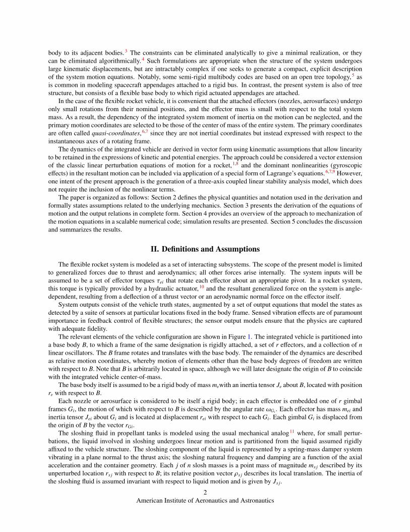
The relevant elements of the vehicle configuration are shown in Figure 1. The integrated vehicle is partitioned intoa base body B, to which a frame of the same designation is rigidly attached, a set of r effectors, and a collection of nlinear oscillators. The B frame rotates and translates with the base body. The remainder of the dynamics are describedas relative motion coordinates, whereby motion of elements other than the base body degrees of freedom are writtenwith respect to B. Note that B is arbitrarily located in space, although we will later designate the origin of B to coincidewith the integrated vehicle center-of-mass.
The base body itself is assumed to be a rigid body of mass mvwith an inertia tensor Jv about B, located with positionrv with respect to B.
Each nozzle or aerosurface is considered to be itself a rigid body; in each effector is embedded one of r gimbalframes Gi, the motion of which with respect to B is described by the angular rate ωGi . Each effector has mass mei andinertia tensor Jei about Gi and is located at displacement rei with respect to each Gi. Each gimbal Gi is displaced fromthe origin of B by the vector rGi.
The sloshing fluid in propellant tanks is modeled using the usual mechanical analog11 where, for small pertur-bations, the liquid involved in sloshing undergoes linear motion and is partitioned from the liquid assumed rigidlyaffixed to the vehicle structure. The sloshing component of the liquid is represented by a spring-mass damper systemvibrating in a plane normal to the thrust axis; the sloshing natural frequency and damping are a function of the axialacceleration and the container geometry. Each j of n slosh masses is a point mass of magnitude ms j described by itsunperturbed location rs j with respect to B; its relative position vector ρs j describes its local translation. The inertia ofthe sloshing fluid is assumed invariant with respect to liquid motion and is given by Js j.
2American Institute of Aeronautics and Astronautics
Figure 1. Flexible vehicle with effector and sloshing mass
Finally, the flexibility of the system is assumed to be in mass-normalized diagonal form; i.e., the orthogonalmodes of a finite element model. The finite element model with p degrees of freedom is described by a vectorgeneralized displacement η ∈ Rp, generalized velocity η ∈ Rp, and a set of associated partial eigenvectors Φk,Ψk ∈
R3×p corresponding to the translational and rotational components of the eigenvectors, respectively, at each discretegridpoint. The p degrees of freedom contain only the vehicle elastic modes; it is assumed that the rigid-body modes(zero-eigenvalued modes) are both orthogonal to the elastic modes and have been removed from the finite elementmodel via an appropriate partitioning procedure.
A summary of the variables describing the system is shown in the following table.
Quantity DescriptionB Body frame, fixed with respect to rigid base body
rGi Location of gimbal frame of each i of r effectors with respect to Bmv, Jv, rv Mass, moment of inertia, and location of vehicle CM with respect to B,
not including effectors and sloshing propellantmei, Jei, rei Mass, moment of inertia, and location of of ith effector with respect to Gi
ms j, Js j, rs j, ρs j Mass, inertia, position, and displacement of each j of n slosh massesη, η Elastic generalized displacement and generalized velocity
Table 1. Dynamical variables
Fundamentally, we assume that certain tensors in B are unchanged with respect to angular displacements. Forexample, the value of an inertia tensor of the ith effector about frame G, coordinated in frame B, varies with thedirection cosines that relate the basis vectors of B and G. The variation is assumed negligible for small rotations. Ifthe two frames are nominally aligned,
JBei = [CBG]JG
ei[CGB] ≈ JG
ei . (1)
In assuming small rotations, the transformation effecting a rotation between two frames A and B is sequence-independentand can be partitioned into a linear form such that
[CBA] = [I + ε×], (2)
where I is the identity and ε× is the skew-symmetric form of the small rotator. We will also use the skew-symmetricform to represent the vector cross-product.6
3American Institute of Aeronautics and Astronautics
In the following section, we derive the equations of motion for the integrated system.
III. Dynamics
The approach to the derivation of the dynamics yields both linear and partial nonlinear forms. First, the kinetic andpotential energies are described in terms of mixed velocities and displacements. Thereafter, the generalized momentaare derived for the composite system. Finally, a state vector is chosen and a special form of Lagrange’s equations inquasi-coordinates is used to derive the equations of motion. The linearized equations of motion follow as a specialcase.
A. Kinetic Energy
The kinetic energy of the integrated system is expressed in mixed coordinates. The kinetic energy of the basebody is expressed in terms of the translational and angular velocities of the B frame, augmented by the energy of theeffectors and slosh masses resulting from their local velocity with respect to B. We will assume for convenience andwithout loss of generality that (1) the finite element associated with each effector has its origin coincident with each Gi
frame and (2) the vehicle and sloshing masses are point masses, to which each has associated a single physical elasticdisplacement but an arbitrary number of elastic coordinates. The latter assumption avoids unnecessary bookkeeping ofintegrals or sums associated with elasticity in either continuum or discrete form, respectively, and makes no differencein the final formulation.
The kinetic energy T is given by the sum of the contributions of the empty vehicle and fixed propellant, sloshingpropellant, and effectors, such that
T = Tv +
n∑j=1
Ts j +
r∑i=1
Tei. (3)
The velocity of the vehicle base body mass in the inertial frame is
vv = vB + Φvη + ω×Brv (4)
where Φv ∈ R3×p. The velocity consists of the reference frame velocity, the velocity due to elastic motion,† and the
velocity due to rotation of the B frame. Likewise, the velocity of a slosh mass in the rotating frame is
vs j = vB + Φs jη + ω×Brs j + ρs j, (5)
and the effector velocity isvei = vB + ΦGiη + ω×B(rGi + rei) + ω×Girei + (ΨGiη)×rei, (6)
where we have accounted for the additional angular velocity of each frame Gi with respect to B.It follows then that the elements of (3) can be expanded as
2Tv = mv(vB + Φvη + ω×Brv
)2
2Ts j = ms j
(vB + Φs jη + ω×Brs j + ρs j
)2(7)
2Tei = mei
(vB + ΦGiη + ω×B(rGi + rei) + ω×Girei + (ΨGiη)×rei
)2
where the operator (.)2 in the vector context is taken to be the appropriate transpose-inner-product operation.
†It is helpful to clarify that the orthogonality of the finite element modes is with respect to motion of the integrated vehicle, not the base body.Therefore, the expression (4) describes the sum of elastic motion of all mass excluding the effectors and slosh masses.
4American Institute of Aeronautics and Astronautics
B. Generalized Momenta
1. Rigid Linear Momentum
From the kinetic energies, the generalized momenta of each subsystem can be calculated. The generalized mo-menta with respect to body frame translation are determined to be
∇vB Tv = mvvB + mvΦvη + mvω×Brv
∇vB Ts j = ms jvB + ms jΦs jη + ms jω×Brs j + ms jρs j (8)
∇vB Tei = meivB + meiΦGiη + meiω×B(rGi + rei) + meiω
×Girei + mei(ΨGiη)×rei
The terms in (8) are grouped such that
∇vB Tv = mvvB − mvr×v ωB + mvΦvη
∇vB Ts j = ms jvB − ms jr×s jωB + ms jρs j + ms jΦs jη (9)∇vB Tei = meivB − mei(rGi + rei)×ωB − meir×eiωGi + meiΦGiη − meir×eiΨGiη;
note that if mv +∑
ms j +∑
mei = mT (total mass) and that if we now assume that B is at the center of mass of theintegrated vehicle,
n∑j=1
ms jrs j +
r∑i=1
mei(rGi + rei) + mvrv = 0, (10)
which, as expected, decouples the translational momentum from the angular momentum since the velocity vB is thatof the center of mass.
We note that momentum is conserved in vibration by virtue of orthogonality, so
mvΦvη +
n∑j=1
ms jΦs jη +
r∑i=1
(meiΦGiη − meir×eiΨGiη) = 0, (11)
and the total linear momentum of the integrated body is
∇vB T = mT vB +
n∑j=1
ms jρs −
r∑i=1
meir×eiωGi. (12)
The last term in (12) is the change in linear momentum due to angular velocity of an attached effector and is thelateral effect of “tail-wags-dog” inertial coupling.
2. Rigid Angular Momentum
The generalized momentum of the body frame with respect to the angular velocity ωB is found to be
∇ωB Tv = mvr×v vB + mvr×v Φvη + mvr×v ω×Brv
∇ωB Ts j = ms jr×s jvB + ms jr×s jΦs jη + ms jr×s jω×Brs j + msr×s jρs j (13)
∇ωB Tei = mei(rGi + rei)×vB + mei(rGi + rei)×ΦGiη
+mei(rGi + rei)×ω×B(rGi + rei)+mei(rGi + rei)×ω×Girei + mei(rGi + rei)×(ΨGiη)×rei.
Thereafter, we group terms and again note that angular momentum is conserved in normal vibration and that theorigin of B is the center of mass. We also employ the identity∑
N
mir×i ω×Bri = JωB. (14)
The resultant simplifications yield
∇ωB Tv = JvωB
∇ωB Ts j = Js jωB + ms jr×s jρs j (15)∇ωB Tei = JeiωB + mei(rGi + rei)×ω×Girei.
5American Institute of Aeronautics and Astronautics
The effector energy can be expanded such that
∇ωB Tei = JeiωB − r×Gimeir×eiωGi + meir×eiω×Girei. (16)
The last term, using (14), is the effector inertia about the gimbal pivot point;
∇ωB Tei = JeiωB + (Jei − r×Gimeir×ei)ωGi. (17)
Then, letting the integrated system inertia be JT = Jv +∑
Js j +∑
Jei, the total angular momentum with respect toB is
∇ωB T = JTωB +
n∑j=1
ms jr×s jρs j +
r∑i=1
(Jei − r×Gimeir×ei)ωGi. (18)
As in the translational case, the last term in (18) is change in angular momentum of the rigid body due to theangular velocity of an attached effector, or the angular effect of “tail-wags-dog.”
3. Momenta Due to Slosh
The generalized momenta with respect to the slosh coordinates are found to be
∇ρs j Tv = 0
∇ρs j Tsσ =
ms jvB + ms jΦs jη + ms jω×Brs j + ms jρs j, j = σ
0, j , σ(19)
∇ρs j Tei = 0.
The total momentum of each sloshing mass is therefore
∇ρs j T = ms jρs j + ms jvB + ms jΦs jη − ms jr×s jωB. (20)
4. Momenta Due to Effectors
The generalized momentum of each effector due to its angular velocity is given by
∇ωGi Tv = 0∇ωGi Ts j = 0
∇ωGi Teσ =
meir×eivB + meir×eiΦGiη + meir×eiω
×B(rGi + rei)
+meir×eiω×Girei + meir×ei(ΨGiη)×rei, i = σ
0, j , σ.(21)
Reordering the terms in (21), it follows that
∇ωGi Tei = JeiωGi + meir×eivB + meir×eiω×B(rGi + rei) + meir×eiΦGiη + meir×ei(ΨGiη)×rei; (22)
noting that meir×eiω×B(rGi + rei) = (Jei − meir×eir
×Gi)ωB, the angular momentum becomes
∇ωGi T = JeiωGi + meir×eivB + (Jei − meir×eir×Gi)ωB + (meir×eiΦGi + JeiΨGi)η. (23)
5. Momenta Due to Bending
The momentum due to bending can be determined as
∇ηTv = ΦvmvvB + ΦvmvΦvη + Φvmvω×Brv
∇ηTs j = Φs jms jvB + Φs jms jΦs jη + Φs jms jω×Brs j + Φs jms jρs j (24)
∇ηTei = ΓeimeivB + ΓeimeiΦGiη + Γeimeiω×B(rGi + rei)
+Γeimeiω×Girei + Γeimei(ΨGiη)×rei
6American Institute of Aeronautics and Astronautics
whereΓei = ΦGi − r×eiΨGi. (25)
This term contains the rotary inertia of the attached nozzle. Assuming again that modal coordinates are orthogonalto rigid body coordinates and that the body frame is fixed at the center of mass,
∇ηTv = ΦvmvΦvη
∇ηTs j = Φs jms jΦs jη + Φs jms jρs j (26)∇ηTei = ΓeimeiΦGiη + Γeimeiω
×Girei + Γeimei(ΨGiη)×rei.
Note that the generalized mass can be defined as
µ = ΦvmvΦv +
n∑j=1
Φs jms jΦs j +
r∑i=1
(ΓeimeiΦGi − Γeimeir×eiΨGi
), (27)
which includes the rotating nozzle masses. Finally, expand the remaining term in (26) as
Γeimeiω×Girei = ΨGimeir×eiω
×Girei − ΦGimeir×eiωGi =
(ΨGiJei − ΦGimeir×ei
)ωGi (28)
and the bending generalized momentum becomes
∇ηT = µη +
n∑j=1
Φs jms jρs j +
r∑i=1
(ΨGiJei − ΦGimeir×ei
)ωGi. (29)
The last term in (29) is the contribution to the bending momentum due to the nozzle angular velocity.
C. Potential Energy and Damping
The system potential accounts for the strain energy due to bending, the potential due to deflection of each sloshmass, and the potential due to the torsional stiffness of each effector rotated around its hinge point. Likewise, theenergy dissipation is a function of the bending generalized velocity, the slosh perturbation velocity, and the angularrate of each effector. The expressions for bending are derived from the well-known second-order linear structuraldynamic model recast in a modal form via a similarity transformation x = Φη such that
ΦMΦη + Dbη + ΦKΦη = Φ f (30)
with ΦMΦ = µ, ΦKΦ = Kb, and some assumed damping matrix Db. While generally µ = I, it is not strictlynecessary that Db,Kb be diagonal or have any particular properties. It is often necessary to admit asymmetric dampingand stiffness that account for aeroelastic coupling effects.12 As can be seen from the developments in Sections (1) and(2), it is only required that the elastic response is orthogonal to the rigid-body degrees of freedom.
It follows that the potential and dissipation functions can be written as
2V = ηKbη +
n∑j=1
ρs jKs jρs j +
r∑i=1
θGiKeiθGi (31)
2D = ¯ηDbη +
n∑j=1
¯ρs jDs jρs j +
r∑i=1
ωGiDeiωGi.
The assumption has been made that∫ωGidt ≈ θGi; kinematics of the nozzle have been ignored on account of small
rotations.
D. Generalized Forces
1. Generalized Forces Due to Effector Motion
The primary exciter of bending, lateral, and angular motion is the generalized force due to thrust or control surfacemoments. Suppose there exists an effector force in the body frame modeled as a unit vector of undeflected force uei
and its associated magnitude Rei. The force in the body frame of the ith effector is
fei = [CBG]Reiuei (32)
7American Institute of Aeronautics and Astronautics
where [CBG] is the kinematic transformation that expresses the rotating unit vector uei in the body frame. If therotations are small with respect to the nominal cant angle, the transformation [CBG] can be partitioned;
fei =[I + θ×Gi + (ΨGiη)×
]Reiuei = Reiuei − Reiu×eiθGi − Reiu×eiΨGiη. (33)
The resultant moment is then
τei = r×Gi fei = r×GiReiuei − r×GiReiu×eiθGi − r×GiReiu×eiΨGiη. (34)
Clearly, there is a static component and a component that is dependent on the generalized coordinates. The ex-pressions (33) and (34) are suitable for modeling a thrusting, gimbaled rocket nozzle. Note that we do not complicatethe dynamics be constraining the rotation θGi to occur about a particular pair of axes; since the nominal cant angleuei can be arbitrary in the body frame, a rotation in the body frame is also, in general, a three-axis rotation. For arocket nozzle, servo torques are applied in the appropriate local pitch-yaw sense (“rock” and “tilt”) via a constantinput transformation that maps the local gimbal coordinate system into the body frame. The nozzle stiffness Kei anddamping Dei are adjusted to approximate the constrained nozzle along the local roll axis in the gimbal frame.
If the effector type is a simple aerosurface, it can also be modeled as a linear angle-dependent moment effector,where Rei is an effectiveness matrix that varies as a function of flight condition.
2. Generalized Forces Due to Aerodynamics
It is straightforward to add a complex nonlinear aerodynamics model using the typical table-lookup method toapply forces to the rigid body degrees of freedom. For stability analysis, it is often necessary to consider perturbationswith respect to a trim condition. In the case of an accelerating rocket, the reference frame is taken to be the acceleratingframe tangent to a gravity turn trajectory. The angle of attack of the vehicle is a function of the vehicle pointing angleθB and lateral velocity vT with respect to the trajectory. For small angles, the transformation from body to trajectory-relative acceleration is given by
vT = vB + θ×BaB (35)
where aB is the vector of instantaneous thrust acceleration expressed in the body frame. The equations of motion arethen transformed to trajectory frame relative motion by inserting the inverse transformation. Thereafter, the linearaerodynamic force and moment on the rigid body are approximated by a set of aerodynamic stiffness and dampingmatrices, where
faero = − (KtrθB + CttvT + CtrωB)
τaero = − (KrrθB + CrtvT + CrrωB) . (36)
The relevant terms embedded therein are a function of dynamic pressure and the 6-DoF linear stability derivatives.
E. Boltzmann-Hamel Equations
The equations of motion of the integrated system can be determined from the generalized momenta and a modifiedform of Lagrange’s equations. Note that the energy has already been expressed in the most convenient form foranalysis. Let us write Lagrange’s equations in the classical form for an unconstrained system;
ddt
(∂L∂qi
)−∂L∂qi
= Qi, (37)
where L = T − V , qi are each generalized coordinate and Qi is the generalized force associated with that coordinate.For this special class of system, we note that ∂T/∂qi = 0; it is sufficient to rewrite (37) in vector form as
ddt
(∇qT
)+ ∇qV = Q. (38)
Without loss of generality, let us choose a state vector of true velocities
q =
vCuΦη
8
American Institute of Aeronautics and Astronautics
where v are holonomic, or integrable velocities, and u are non-holonomic or quasi-velocities. The transformation Cis the orthonormal kinematic transformation that coordinates the non-holonomic velocities u in the inertial frame, andthe transformation Φ is the orthonormal linear transformation that maps elastic generalized velocities η into physicalvelocities.
The direct vector form of Lagrange’s equation applies to the holonomic velocities, and observing that there are noposition-dependent potential terms,
ddt
(∇vT ) = Qv. (39)
In the case of the quasi-velocities u, we substitute the transformed coordinates into (38) and find that
Cddt
(∇uT ) + C∇uT + ∇ξV = Qu (40)
where ξ = Cu. Recall that C relates an inertial to a rotating frame and is always orthonormal, so CC = I. The timederivative C = Cω×B and equation (40) can be written as
ddt
(∇uT ) + ω×B∇uT + C∇ξV = CQu. (41)
Finally, we consider the elastic velocities’ contribution to the kinetic and potential energies. The elastic physicalvelocities are orthogonalized via some constant linear transformation. The elastic velocities are indeed relative motioncoordinates with respect to the rotating frame, but they are coordinated with respect to an inertial basis. The elasticcoordinates are therefore holonomic coordinates. Physically, the structural displacements must coincide with theundeformed rigid body, which follows from assumption that the rigid body modes are to be excluded from the elasticsolution.
Since Lagrange’s equations for the elastic coordinates undergo only a constant transformation, we have that
Φddt
(∇ηT
)+ Φ∇ηV = Qη (42)
and, with ΦΦ = I, the flexibility equations have the expected classical form
ddt
(∇ηT
)+ ∇ηV = ΦQη. (43)
The expressions (39), (41), and (43) are a special vector form of the Boltzmann-Hamel equations, or Lagrange’sequations in quasi-coordinates.9 They are much simplified compared to the more general forms of the Boltzmann-Hamel equations.
9American Institute of Aeronautics and Astronautics
F. Equations of Motion
The time-invariant equations of motion in final form follow directly from the generalized momenta and the appli-cation of the Boltzmann-Hamel equations. Under the previously stated kinematic and dynamic modeling assumptions,the complete trajectory-relative motion equations are given below.
Translation
mT vT = mT θ×BaB −
∑n
j=1ms jρs −
∑n
j=1ms jω
×Bρs +
∑r
i=1(meir×eiωGi)
+∑r
i=1Rei
(uei − u×eiθGi − u×eiΨGiη
)− (KtrθB + CttvT + CtrωB) (44)
Rotation
JT ωB = −∑n
j=1ms jr×s jρs j −
∑r
i=1(Jei − r×Gimeir×ei)ωGi
− ω×B(JTωB +
∑r
i=1(Jei − r×Gimeir×ei)ωGi
)+
∑r
i=1Rei
(r×Giuei − r×Giu
×eiθGi − r×Giu
×eiΨGiη
)− (KrrθB + CrtvT + CrrωB) (45)
Slosh ( j = 1, 2, . . . n)
ρs j + Ds jρs j + Ks jρs j = −vB − Φs jη + r×s jωB − ω×B
(2ρs j + vB + Φs jη − r×s jωB
)(46)
Nozzle (i = 1, 2, . . . , r)
JeiωGi + DeiωGi + KeiθGi = τei − meir×eivB − (Jei − meir×eir×Gi)ωB − (meir×eiΦGi + JeiΨGi)η
− ω×B(JeiωGi + meir×eivB + (Jei − meir×eir
×Gi)ωB
)− ω×B(meir×eiΦGi + JeiΨGi)η (47)
Bending
µη + Dbη + Kbη = −∑n
j=1Φs jms j(ρs j + ω×Bρs j) −
∑r
i=1
(ΨGiJei − ΦGimeir×ei
)ωGi
+∑r
i=1ReiΦGi
(uei − u×eiθGi − u×eiΨGiη
)(48)
In the full nonlinear form given above, the motion equations are easily integrated into a trajectory simulation viapartitioning into the requisite generalized mass matrix E. In time-invariant form, the linear components are readilymechanized into a first-order descriptor form by writing the linear dynamics as
Ex = Ax + Bu (49)y = Cx + Du
with the state vector
x =
[θB θG1 θG2 . . . θGr ρs1 ρs2 . . . ρsn η
]T[vB ωB ωG1 ωG2 . . . ωGr ¯ρs1 ¯ρs2 . . . ¯ρsn ¯η
]T
. (50)
Linear models of the flight control system and the servoactuators are block-diagonalized with the plant dynamicsmodel and the multiple-input, multiple-output (MIMO) frequency response and eigenvalues can be computed numer-ically using commonly available computational tools.
10American Institute of Aeronautics and Astronautics
G. Output Models
The system outputs capture the effects of sensor mounting on an arbitrary point on the structure. We assumethat the sensor output axes are nominally aligned with the body axes. Sensor types to be considered in the presentapplication are rate gyros, integrating gyros (attitude angle sensors), and accelerometers.
Each attitude angle and rate sensor detects the superposition of the body attitude with the corruption due to elasticmotion, given by
θm = θB + Ψymη (51)ωBm = ωB + Ψymη
where Ψym ∈ R3×p is the subset of column eigenvectors associated with rotation at the mth sensor.
The accelerometer sensor includes the linear effects of local rotation and the nonlinear effects due to non-colocationwith the center of mass. If rym is the vector from the center of mass to the sensor in the body frame, the sensedacceleration with respect to the reference frame is
γym = [CYB](vB + rym + 2ω×Brym + ω×Brym + ω×Bω
×Brym
).
Note that due to flexibility, the transformation [CYB] rotates the sensed body acceleration through small angles;also, the sensor velocity and acceleration with respect to the center of mass are a function of the elastic generalizedcoordinates. We neglect the small velocity of the sensor relative to the center of mass due to burning propellant. Itfollows that
γym =[I + (Ψymη)×
] (vB + ω×Brym + ω×Bω
×Brym + Φymη + 2ω×BΦymη
). (52)
In most applications, we can safely ignore the higher-order flexibility terms and model the accelerometer as
γym = vB + ω×Brym + ω×Bω×Brym − v
×BΨymη + 2ω×BΦymη + Φymη. (53)
IV. Simulation
The present formulation has been incorporated into a general missile autopilot stability analysis and design tool,FRACTAL (Frequency Response Analysis and Comparison Tool Assuming Linearity). FRACTAL is a scalable im-plementation of the equations of motion that allows the trajectory to be simulated at a various flight conditions underthe assumptions of fixed (linear, time-invariant) or time-varying parameters so as to assess the impact of parametricuncertainty in a given vehicle configuration. While the current mechanization now allows full nonlinear trajectorysimulation in the software, FRACTAL’s primary analysis task is the generation of time and frequency domain resultsto characterize the stability characteristics of the integrated system using linear control system stability metrics.
Owing to the easily implemented matrix-vector form of the equations of motion, numerical assembly of linear sys-tems representing the full vehicle dynamics with autopilot and actuators in-the-loop is exceptionally rapid on moderncomputing hardware. The software is equipped to automatically construct the equations of motion to arbitrary scale upto the limits of memory and computational capacity; for example, a typical FRACTAL linear model of a five-engineheavy-lift launcher concept may have as many as 260 states. The efficient form of the equations of motion makesthe model particularly well suited to numerical optimization of the flight control system design parameters, whichemploys extensive finite differencing implemented in a parallel computing environment.
Validation
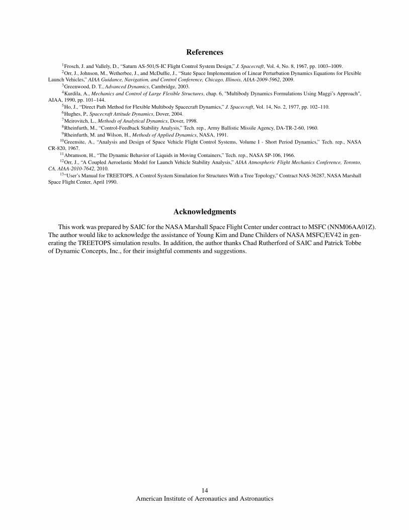
Various simulation test cases have been constructed to compare the response of the present formulation with well-established and validated dynamics models. A time-domain test case example is shown below in Figures 2 and 3,where the FRACTAL model dynamics are a trajectory-relative perturbation model. The results have been comparedto TREETOPS,13 a multi-body dynamics package based on Kane’s equations.3 In the simulation results shown, anexample system consisting of a rigid vehicle with an attached nozzle is assembled together with a pair of linearservoactuators that provide torques about the nozzle in the pitch and yaw axes. The vehicle gimbal angle command isexcited with a small-amplitude sinusoidal wavelet to verify the coupled response of the thrusting engine, the actuators,and the vehicle to which they are attached. With small angles and small body rates, gyroscopic coupling is minimaland the models agree exceptionally well even considering the omitted nonlinearities.
11American Institute of Aeronautics and Astronautics
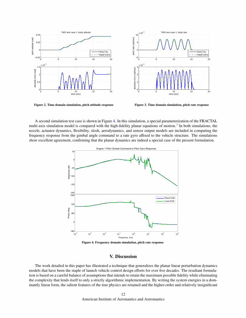
0 5 10 15 20−0.02
0
0.02
0.04pi
tch
attit
ude
(rad
)TWD test case 1: body attitude
FRACTALTREETOPS
0 5 10 15 200
0.5
1
1.5x 10
−5
time (sec)
abso
lute
err
or (
rad)
Figure 2. Time domain simulation, pitch attitude response
0 5 10 15 20−5
0
5
10x 10
−3
pitc
h ra
te (
rad/
sec)
TWD test case 1: body rate
FRACTALTREETOPS
0 5 10 15 200
1
2
3x 10
−5
time (sec)
abso
lute
err
or (
rad/
sec)
Figure 3. Time domain simulation, pitch rate response
A second simulation test case is shown in Figure 4. In this simulation, a special parameterization of the FRACTALmulti-axis simulation model is compared with the high-fidelity planar equations of motion.2 In both simulations, thenozzle, actuator dynamics, flexibility, slosh, aerodynamics, and sensor output models are included in computing thefrequency response from the gimbal angle command to a rate gyro affixed to the vehicle structure. The simulationsshow excellent agreement, confirming that the planar dynamics are indeed a special case of the present formulation.
-200
-150
-100
-50
0
50
Mag
nitu
de
(d
B)
10-4
10-3
10-2
10-1
100
101
102
103
-360
0
360
720
1080
Pha
se (
de
g)
Frequency (Hz)
Engine 1 Pitch Gimbal Command to Pitch Gyro Response
Planar EoM
3-axis EoM
Figure 4. Frequency domain simulation, pitch rate response
V. Discussion
The work detailed in this paper has illustrated a technique that generalizes the planar linear perturbation dynamicsmodels that have been the staple of launch vehicle control design efforts for over five decades. The resultant formula-tion is based on a careful balance of assumptions that intends to retain the maximum possible fidelity while eliminatingthe complexity that lends itself to only a strictly algorithmic implementation. By writing the system energies in a dom-inantly linear form, the salient features of the true physics are retained and the higher-order and relatively insignificant
12American Institute of Aeronautics and Astronautics

kinematic effects have been omitted. Most importantly, the formulation leads to an explicit and intuitive set of motionequations that are easily coded in both linear and nonlinear forms. The model has direct applications to Monte Carlosimulation, stability analysis, and numerical optimization, and is extensible to a wide variety of vehicle configurations,including launch vehicles, missiles, and thrust-vector-controlled aircraft.
13American Institute of Aeronautics and Astronautics
References1Frosch, J. and Vallely, D., “Saturn AS-501/S-IC Flight Control System Design,” J. Spacecraft, Vol. 4, No. 8, 1967, pp. 1003–1009.2Orr, J., Johnson, M., Wetherbee, J., and McDuffie, J., “State Space Implementation of Linear Perturbation Dynamics Equations for Flexible
Launch Vehicles,” AIAA Guidance, Navigation, and Control Conference, Chicago, Illinois, AIAA-2009-5962, 2009.3Greenwood, D. T., Advanced Dynamics, Cambridge, 2003.4Kurdila, A., Mechanics and Control of Large Flexible Structures, chap. 6, "Multibody Dynamics Formulations Using Maggi’s Approach",
AIAA, 1990, pp. 101–144.5Ho, J., “Direct Path Method for Flexible Multibody Spacecraft Dynamics,” J. Spacecraft, Vol. 14, No. 2, 1977, pp. 102–110.6Hughes, P., Spacecraft Attitude Dynamics, Dover, 2004.7Meirovitch, L., Methods of Analytical Dynamics, Dover, 1998.8Rheinfurth, M., “Control-Feedback Stability Analysis,” Tech. rep., Army Ballistic Missile Agency, DA-TR-2-60, 1960.9Rheinfurth, M. and Wilson, H., Methods of Applied Dynamics, NASA, 1991.
10Greensite, A., “Analysis and Design of Space Vehicle Flight Control Systems, Volume I - Short Period Dynamics,” Tech. rep., NASACR-820, 1967.
11Abramson, H., “The Dynamic Behavior of Liquids in Moving Containers,” Tech. rep., NASA SP-106, 1966.12Orr, J., “A Coupled Aeroelastic Model for Launch Vehicle Stability Analysis,” AIAA Atmospheric Flight Mechanics Conference, Toronto,
CA, AIAA-2010-7642, 2010.13“User’s Manual for TREETOPS, A Control System Simulation for Structures With a Tree Topology,” Contract NAS-36287, NASA Marshall
Space Flight Center, April 1990.
Acknowledgments
This work was prepared by SAIC for the NASA Marshall Space Flight Center under contract to MSFC (NNM06AA01Z).The author would like to acknowledge the assistance of Young Kim and Dane Childers of NASA MSFC/EV42 in gen-erating the TREETOPS simulation results. In addition, the author thanks Chad Rutherford of SAIC and Patrick Tobbeof Dynamic Concepts, Inc., for their insightful comments and suggestions.
14American Institute of Aeronautics and Astronautics
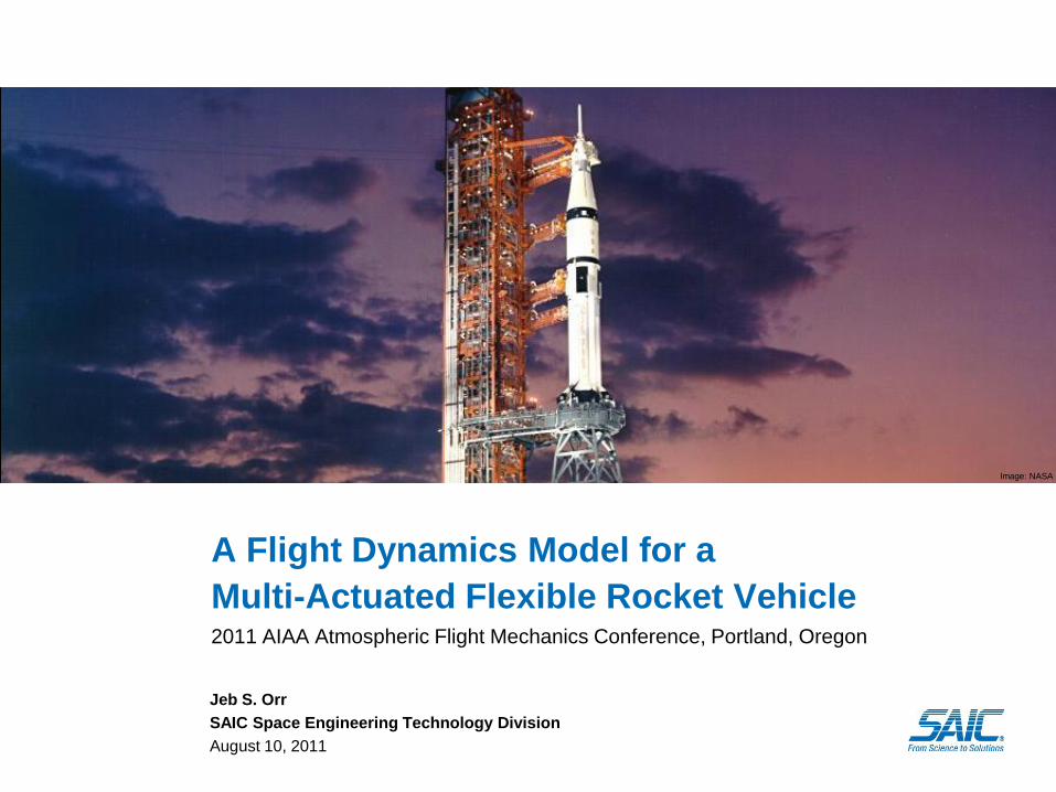
Image: NASA
A Flight Dynamics Model for a
Multi-Actuated Flexible Rocket Vehicle2011 AIAA Atmospheric Flight Mechanics Conference, Portland, Oregon
Jeb S. Orr
SAIC Space Engineering Technology Division
August 10, 2011

Energy | Environment | National Security | Health | Critical Infrastructure
© Science Applications International Corporation. All rights reserved. SAIC and the SAIC logo are registered trademarks of Science Applications International Corporation in the U.S. and/or other countries.
2
Agenda
• Motivation
• Modeling Assumptions
• Modeling Approach
• Verification Results
• Conclusions and Forward Work
Energy | Environment | National Security | Health | Critical Infrastructure
© Science Applications International Corporation. All rights reserved. SAIC and the SAIC logo are registered trademarks of Science Applications International Corporation in the U.S. and/or other countries.
3
Motivation
• Future launch vehicles to be considered for development are not planar,
single- or lumped-nozzle launch vehicles (LVs)
• Ascent flight control design and dynamic modeling for asymmetric systems is
a challenging design task (for example, Shuttle)
• Vehicle may be inertially, elastically, and aerodynamically asymmetric, with
multiple nozzles/effectors of varying types
• No easy-to-use, integrated simulation environment exists for modeling these
systems that can be simultaneously used for flight control design and stability
analysis as well as high-fidelity nonlinear dynamic simulation
• Existing multiple-degree of freedom multiple-body dynamic simulation tools
are not always the best choice
• Classical perturbation equations are high fidelity, but only for planar and
inertially symmetric systems
Energy | Environment | National Security | Health | Critical Infrastructure
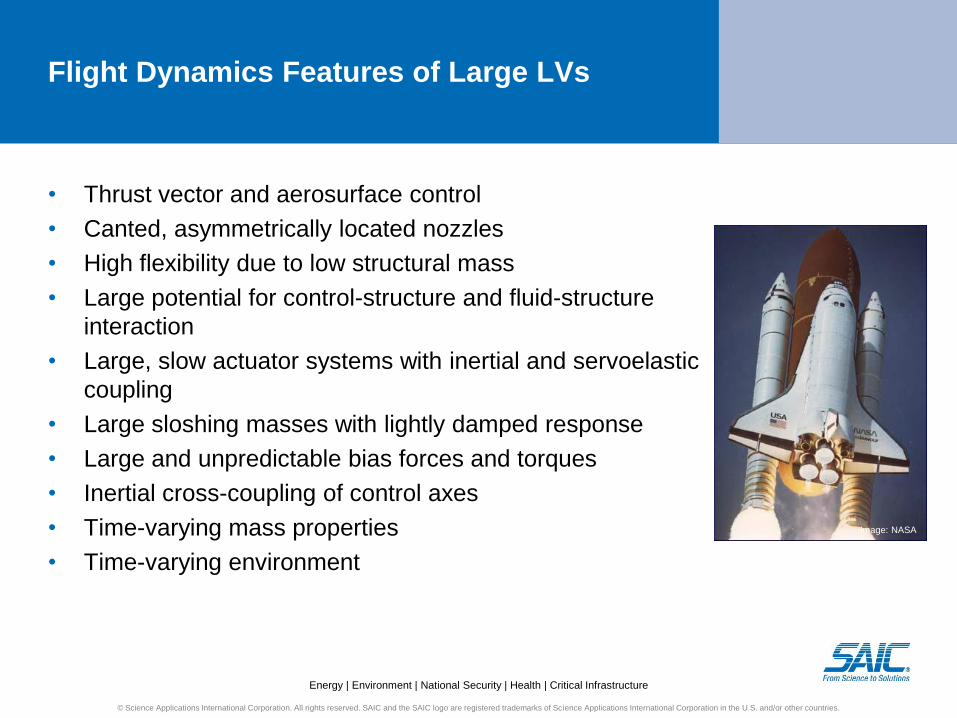
Flight Dynamics Features of Large LVs
• Thrust vector and aerosurface control
• Canted, asymmetrically located nozzles
• High flexibility due to low structural mass
• Large potential for control-structure and fluid-structure
interaction
• Large, slow actuator systems with inertial and servoelastic
coupling
• Large sloshing masses with lightly damped response
• Large and unpredictable bias forces and torques
• Inertial cross-coupling of control axes
• Time-varying mass properties
• Time-varying environment
Image: NASA
© Science Applications International Corporation. All rights reserved. SAIC and the SAIC logo are registered trademarks of Science Applications International Corporation in the U.S. and/or other countries.
Energy | Environment | National Security | Health | Critical Infrastructure
A New Formulation
• We propose a new flight mechanics formulation based on a vector extension
of the classical perturbation equations for launch vehicles
• Nozzle and aerosurface inertial coupling, sloshing propellant, and elasticity
are generalized in the model
• Derived from a rigorous energy-based approach that leverages well-founded
assumptions to minimize the formulation’s complexity
• Results in a closed-form set of motion equations
– A nonlinear simulation can be formed from Lagrange’s equations in
quasicoordinates (the Boltzmann-Hamel equations) to propagate the trajectory
– The linear equations can be directly used to form a state model of the system
dynamics for control design
© Science Applications International Corporation. All rights reserved. SAIC and the SAIC logo are registered trademarks of Science Applications International Corporation in the U.S. and/or other countries.
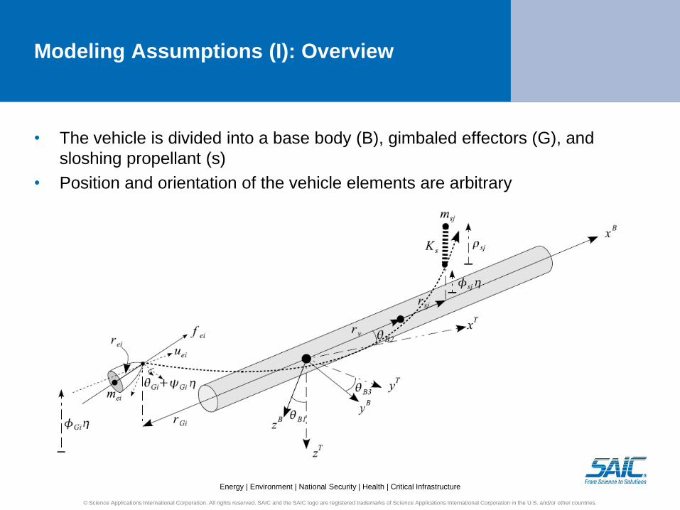
Energy | Environment | National Security | Health | Critical Infrastructure
• The vehicle is divided into a base body (B), gimbaled effectors (G), and
sloshing propellant (s)
• Position and orientation of the vehicle elements are arbitrary
Modeling Assumptions (I): Overview
© Science Applications International Corporation. All rights reserved. SAIC and the SAIC logo are registered trademarks of Science Applications International Corporation in the U.S. and/or other countries.
Energy | Environment | National Security | Health | Critical Infrastructure
Modeling Assumptions (II) : Integrated Vehicle
• External generalized forces are due to thrust and aerodynamics
• Model inputs are a set of effector torques that rotate nozzles/aerosurfaces
• Model outputs are truth states and a set of sensor outputs at arbitrary
locations on the body frame
• All elements are coordinated in the body frame and undergo small
rotations/displacements (nonlinear kinematics are negligible)
– Launch vehicle-specific assumption; not well-suited to spacecraft with flexible
appendages or deployable masts
– Change in integrated MOI due to effector motion is small
• Vehicle mass properties vary slowly enough that higher-order effects due to
element time derivatives are ignored
© Science Applications International Corporation. All rights reserved. SAIC and the SAIC logo are registered trademarks of Science Applications International Corporation in the U.S. and/or other countries.
MOI = moment of inertia
Energy | Environment | National Security | Health | Critical Infrastructure
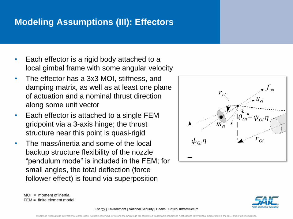
Modeling Assumptions (III): Effectors
• Each effector is a rigid body attached to a
local gimbal frame with some angular velocity
• The effector has a 3x3 MOI, stiffness, and
damping matrix, as well as at least one plane
of actuation and a nominal thrust direction
along some unit vector
• Each effector is attached to a single FEM
gridpoint via a 3-axis hinge; the thrust
structure near this point is quasi-rigid
• The mass/inertia and some of the local
backup structure flexibility of the nozzle
“pendulum mode” is included in the FEM; for
small angles, the total deflection (force
follower effect) is found via superposition
© Science Applications International Corporation. All rights reserved. SAIC and the SAIC logo are registered trademarks of Science Applications International Corporation in the U.S. and/or other countries.
MOI = moment of inertia
FEM = finite element model
Energy | Environment | National Security | Health | Critical Infrastructure
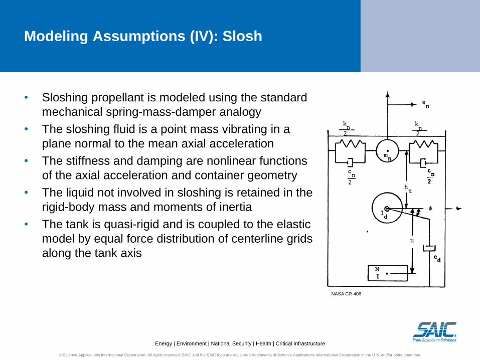
Modeling Assumptions (IV): Slosh
• Sloshing propellant is modeled using the standard
mechanical spring-mass-damper analogy
• The sloshing fluid is a point mass vibrating in a
plane normal to the mean axial acceleration
• The stiffness and damping are nonlinear functions
of the axial acceleration and container geometry
• The liquid not involved in sloshing is retained in the
rigid-body mass and moments of inertia
• The tank is quasi-rigid and is coupled to the elastic
model by equal force distribution of centerline grids
along the tank axis
NASA CR-406
© Science Applications International Corporation. All rights reserved. SAIC and the SAIC logo are registered trademarks of Science Applications International Corporation in the U.S. and/or other countries.
Energy | Environment | National Security | Health | Critical Infrastructure
Modeling Assumptions (V): Elasticity
• The elasticity of the integrated system is modeled as a set of linear orthogonal
modes of a FEM; rigid-body modes are removed via partitioning
• If the FEM is provided at discrete times, the non-orthogonality (with respect to
the rigid body) of mass integrals at other mass configurations is considered
negligible
• The FEM stiffness and damping matrices need not be symmetric, positive
definite, or have any particular properties
• Aeroelastic effects are integrated directly via modification of the stiffness at
damping matrices as a function of flight condition
© Science Applications International Corporation. All rights reserved. SAIC and the SAIC logo are registered trademarks of Science Applications International Corporation in the U.S. and/or other countries.
FEM = finite element model
Energy | Environment | National Security | Health | Critical Infrastructure
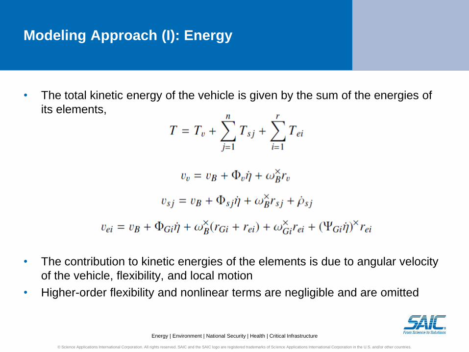
Modeling Approach (I): Energy
• The total kinetic energy of the vehicle is given by the sum of the energies of
its elements,
• The contribution to kinetic energies of the elements is due to angular velocity
of the vehicle, flexibility, and local motion
• Higher-order flexibility and nonlinear terms are negligible and are omitted
© Science Applications International Corporation. All rights reserved. SAIC and the SAIC logo are registered trademarks of Science Applications International Corporation in the U.S. and/or other countries.
Energy | Environment | National Security | Health | Critical Infrastructure
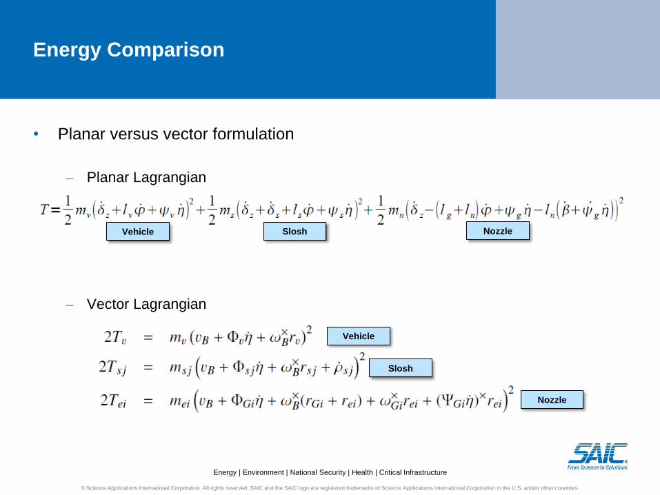
Energy Comparison
• Planar versus vector formulation
– Planar Lagrangian
– Vector Lagrangian
Vehicle Slosh Nozzle
Vehicle
Slosh
Nozzle
© Science Applications International Corporation. All rights reserved. SAIC and the SAIC logo are registered trademarks of Science Applications International Corporation in the U.S. and/or other countries.
Energy | Environment | National Security | Health | Critical Infrastructure
Modeling Approach (II): Generalized Momenta
• The generalized momenta follow from the kinetic energy:
• The time-derivative of the momenta can be readily assembled into the
generalized mass matrix
• Each term is readily associated with a physical phenomena
© Science Applications International Corporation. All rights reserved. SAIC and the SAIC logo are registered trademarks of Science Applications International Corporation in the U.S. and/or other countries.
Energy | Environment | National Security | Health | Critical Infrastructure
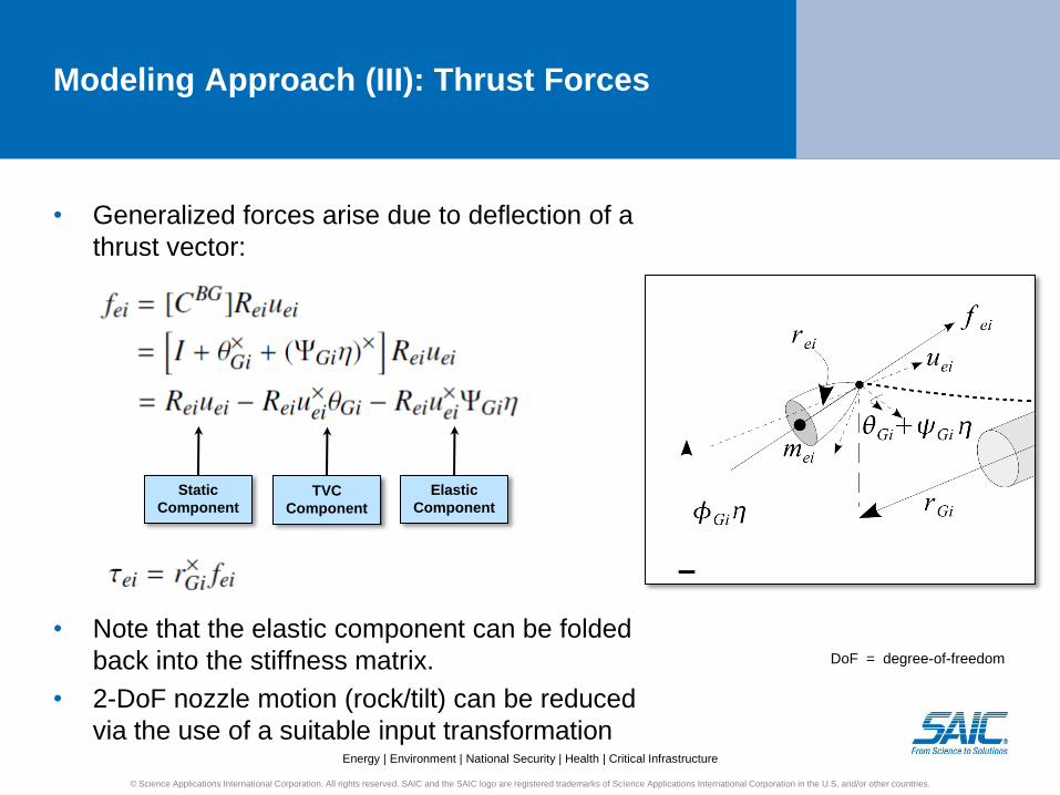
Modeling Approach (III): Thrust Forces
• Generalized forces arise due to deflection of a
thrust vector:
• Note that the elastic component can be folded
back into the stiffness matrix.
• 2-DoF nozzle motion (rock/tilt) can be reduced
via the use of a suitable input transformation
Static
ComponentTVC
Component
Elastic
Component
© Science Applications International Corporation. All rights reserved. SAIC and the SAIC logo are registered trademarks of Science Applications International Corporation in the U.S. and/or other countries.
DoF = degree-of-freedom
Energy | Environment | National Security | Health | Critical Infrastructure
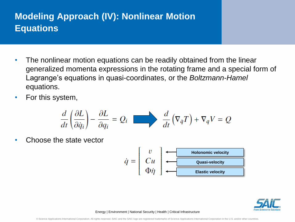
Modeling Approach (IV): Nonlinear Motion
Equations
• The nonlinear motion equations can be readily obtained from the linear
generalized momenta expressions in the rotating frame and a special form of
Lagrange’s equations in quasi-coordinates, or the Boltzmann-Hamel
equations.
• For this system,
• Choose the state vector
Holonomic velocity
Quasi-velocity
Elastic velocity
© Science Applications International Corporation. All rights reserved. SAIC and the SAIC logo are registered trademarks of Science Applications International Corporation in the U.S. and/or other countries.
Energy | Environment | National Security | Health | Critical Infrastructure
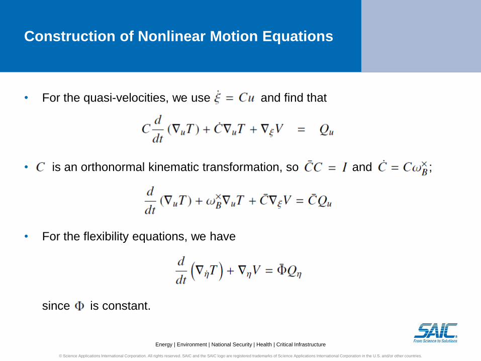
Construction of Nonlinear Motion Equations
• For the quasi-velocities, we use and find that
• is an orthonormal kinematic transformation, so and ;
• For the flexibility equations, we have
since is constant.
© Science Applications International Corporation. All rights reserved. SAIC and the SAIC logo are registered trademarks of Science Applications International Corporation in the U.S. and/or other countries.
Energy | Environment | National Security | Health | Critical Infrastructure
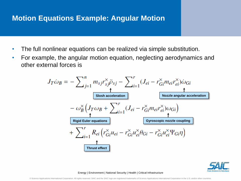
Motion Equations Example: Angular Motion
• The full nonlinear equations can be realized via simple substitution.
• For example, the angular motion equation, neglecting aerodynamics and
other external forces is
Slosh acceleration Nozzle angular acceleration
Rigid Euler equations Gyroscopic nozzle coupling
Thrust effect
© Science Applications International Corporation. All rights reserved. SAIC and the SAIC logo are registered trademarks of Science Applications International Corporation in the U.S. and/or other countries.
Energy | Environment | National Security | Health | Critical Infrastructure
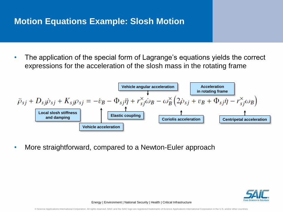
Motion Equations Example: Slosh Motion
• The application of the special form of Lagrange’s equations yields the correct
expressions for the acceleration of the slosh mass in the rotating frame
• More straightforward, compared to a Newton-Euler approach
Local slosh stiffness
and damping
Vehicle acceleration
Elastic coupling
Vehicle angular acceleration
Coriolis acceleration Centripetal acceleration
Acceleration
in rotating frame
© Science Applications International Corporation. All rights reserved. SAIC and the SAIC logo are registered trademarks of Science Applications International Corporation in the U.S. and/or other countries.
Energy | Environment | National Security | Health | Critical Infrastructure
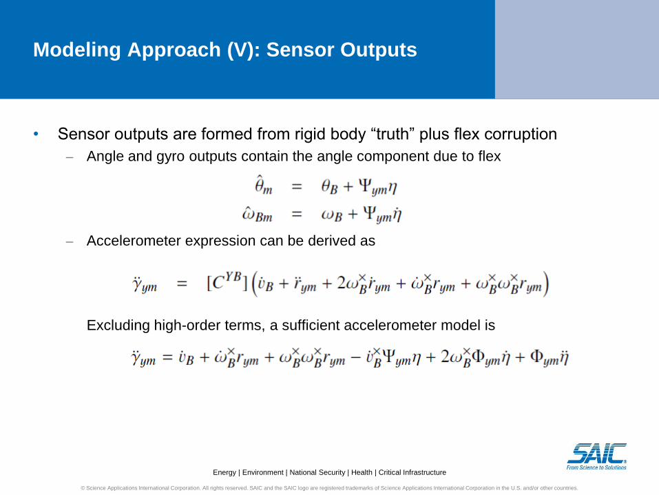
Modeling Approach (V): Sensor Outputs
• Sensor outputs are formed from rigid body “truth” plus flex corruption
– Angle and gyro outputs contain the angle component due to flex
– Accelerometer expression can be derived as
Excluding high-order terms, a sufficient accelerometer model is
© Science Applications International Corporation. All rights reserved. SAIC and the SAIC logo are registered trademarks of Science Applications International Corporation in the U.S. and/or other countries.
Energy | Environment | National Security | Health | Critical Infrastructure
Model Implementation and Verification Activity
• The present model has been integrated into the generalized dynamic
simulation, autopilot design, and stability analysis tool FRACTAL (Frequency
Response Analysis and Comparison Tool Assuming Linearity).
• FRACTAL began as a planar perturbation tool but now implements the full-
featured nonlinear dynamics with an analytic linearization capability.
• Analytic linearizations can be used in parallelizable optimization algorithms for
flight control gain and bending filter design routines.
• High-order (>250 state) linear systems can be automatically generated with
all actuator dynamics and autopilot dynamics included.
• Verification test cases were constructed against the previously, rigorously
exercised classical planar dynamics.
• For special parameterizations, the three-axis model can be made to simulate
a planar vehicle as a special case.
• Time-domain verification against Kane’s equations was also performed.
© Science Applications International Corporation. All rights reserved. SAIC and the SAIC logo are registered trademarks of Science Applications International Corporation in the U.S. and/or other countries.
Energy | Environment | National Security | Health | Critical Infrastructure
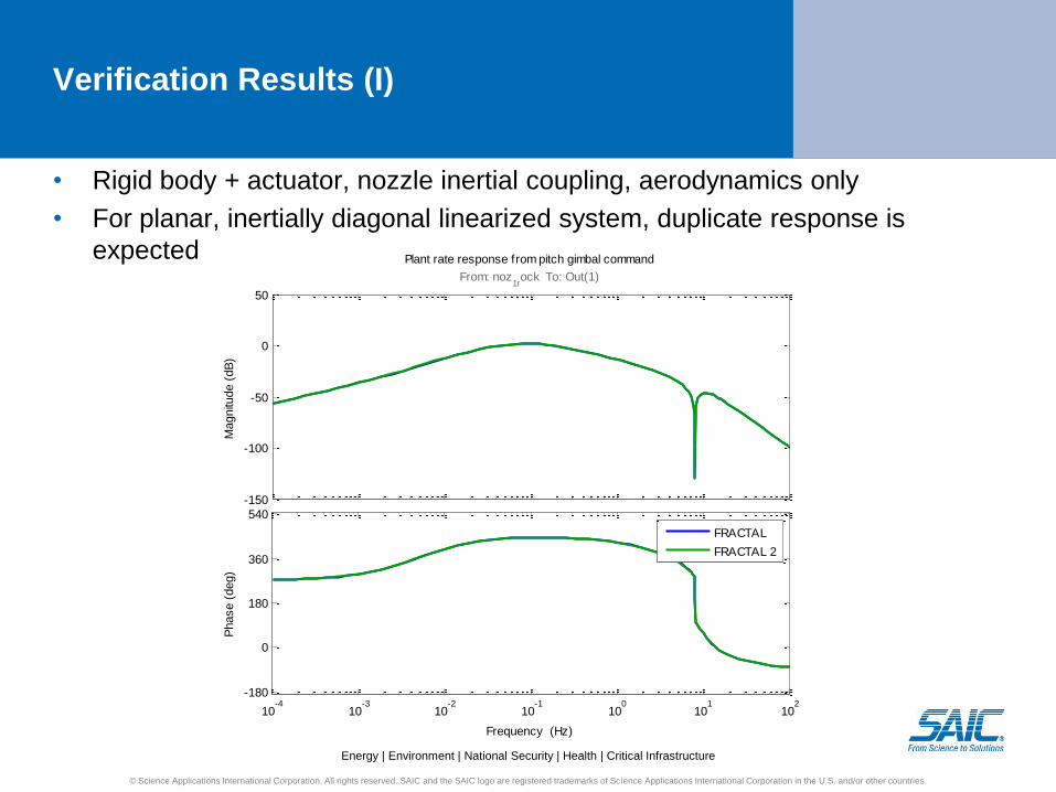
Verification Results (I)
• Rigid body + actuator, nozzle inertial coupling, aerodynamics only
• For planar, inertially diagonal linearized system, duplicate response is
expected
-150
-100
-50
0
50
From: noz1r
ock To: Out(1)
Magnitu
de (
dB
)
10-4
10-3
10-2
10-1
100
101
102
-180
0
180
360
540
Phase (
deg)
Plant rate response from pitch gimbal command
Frequency (Hz)
FRACTAL
FRACTAL 2
© Science Applications International Corporation. All rights reserved. SAIC and the SAIC logo are registered trademarks of Science Applications International Corporation in the U.S. and/or other countries.
Energy | Environment | National Security | Health | Critical Infrastructure
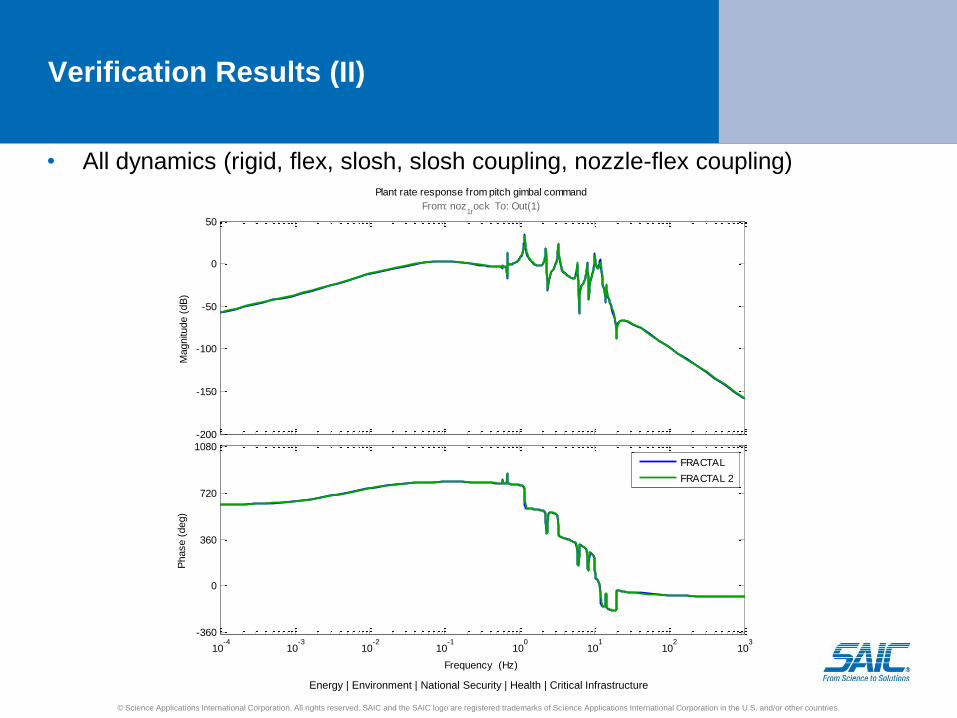
Verification Results (II)
• All dynamics (rigid, flex, slosh, slosh coupling, nozzle-flex coupling)
-200
-150
-100
-50
0
50
From: noz1r
ock To: Out(1)
Magnitu
de (
dB
)
10-4
10-3
10-2
10-1
100
101
102
103
-360
0
360
720
1080
Phase (
deg)
Plant rate response from pitch gimbal command
Frequency (Hz)
FRACTAL
FRACTAL 2
© Science Applications International Corporation. All rights reserved. SAIC and the SAIC logo are registered trademarks of Science Applications International Corporation in the U.S. and/or other countries.
Energy | Environment | National Security | Health | Critical Infrastructure
Summary and Forward Work
• The classical planar equations of motion, based on verified assumptions for
launch vehicle dynamics, have been extended into a fully coupled, nonlinear,
multiple degree-of-freedom set of motion equations.
• The compact form of the final motion equations is easily coded.
• The motion equations can be analytically linearized without resorting to
numerical perturbation methods.
• The code is suitable for any flexible flight vehicle with thrust-vector or
aerosurface control and sloshing propellant, including launch vehicles,
aircraft, and missiles.
• Forward work will examine higher-fidelity time-domain simulation test cases to
quantify the loss of fidelity due to kinematic assumptions.
• The present model is being used as a foundation for additional research into
high-efficiency control allocation algorithms and stability theory for flight
vehicle adaptive control.
© Science Applications International Corporation. All rights reserved. SAIC and the SAIC logo are registered trademarks of Science Applications International Corporation in the U.S. and/or other countries.
Related Documents