A finite-volume solver for two-fluid flow in heterogeneous porous media based on OpenFOAM(R)

A finite-volume solver for two-fluid flow in heterogeneous porous

media based on OpenFOAM R©

O. F. Oxtoby∗, J. A. Heyns and R. Suliman

Aeronautic Systems, Council for Scientific and Industrial Research, Pretoria, South Africa

Abstract

In this paper we derive a finite-volume algorithm for simulating two-fluid flows in

porous media. The algorithm handles arbitrary heterogeneous porosity fields contain-

ing discontinuities without introducing instabilities or oscillations into the solution. For

the two-fluid (free-surface) modelling the volume of fluid (VoF) method is used with the

HiRAC interface capturing algorithm. The developed scheme is evaluated by comparison

with high-fidelity experimental results and found to agree well. The scheme is implemented

in the OpenFOAM R© code and extends upon the capabilities contained therein.

1 Introduction

Packed beds and multiphase flows are two common features of industrial processes such as

furnaces [1] and reactor vessels [2], and yet the combination of the two is spasely covered by

the literature on numerical modelling. Further applications include wave action on harbour

breakwaters [3] and multi-fluid flows in rock beds, which encompasses the forced extraction of

oil in underground wells as well as sparging of non-aqueous pollutants [4].

In this paper our aim is to derive a numerical method for handling arbitrary heterogeneous

porosity fields, including possible discontinuities, without introducing instabilities or spurious

oscillations. At present, only homogeneous porous zones are catered for by the OpenFOAM R©

software; however, implementation of the methods presented below allows porosity to be spec-

ified as just another field, and set up using the standard tools, for example the setFields

utility.

The outline of this paper is as follows. In Section 2, the governing equations for porous multi-

phase flows are presented, then in Section 3 their discresation is derived, including the consis-

tent handling of discontinuities. Finally, Section 4 describes the evaluation problem to which

the algorithm is applied.

∗E-mail: [email protected]

1

2 Model Equations

The physical domain to be modelled contains two immiscible viscous incompressible fluids

present in the pores between a solid matrix. Initially, we focus on the fluid regions only. For

clarity, we shall refer to the two fluids as liquid and gas, although the same arguments also apply

unmodified for fluids of the same phase. For modelling purposes we may make the assumption

that there is a small mixed region where the fluids meet, and assume a continuous pressure and

velocity field. We define an indicator fraction α as

α = 1 in the liquid phase,

α = 0 in the gas phase, and

0 < α < 1 in the notional smooth transition region.

(1)

By considering mass conservation of the two fluids, one obtains, firstly, the standard incom-

pressible divergence-free constraint,

∂ui

∂xi

= 0, (2)

where ui are the components of velocity. Secondly, one obtains the interface-convection equa-

tion

∂α

∂t+

∂

∂xi

(αui) = 0. (3)

Interface-capturing algorithms are necessary to maintain the sharpness of the nearly-discontinuous

volume-fraction field α, i.e. to keep the fictional transition region between the two fluids as small

as the discretisation method will allow. This will be detailed in Section 3.1 below.

Considering now the conservation of momentum in the liquid/gas continuum, we obtain the

standard momentum equation

∂ρuj

∂t+

∂

∂xi

(ρuiuj) +∂p

∂xj

=∂

∂xi

[

µ

(

∂ui

∂xj

+∂uj

∂xi

)]

+ ρgj. (4)

Here, ρ = αρl + (1 − α)ρg and µ = αµl + (1 − α)µg are the effective material properties of

the mixture, where ρl, µl and ρg, µg are the density and viscosity of the liquid and gas phase

respectively, gj denotes the body-force acceleration in direction j and p represents the pressure

field. Due to the sharp density gradients inside the convective terms, the numerical treatment of

this equation is delicate. To avoid this, several authors [5, 6, 7, 8] use an alternative formulation

of momentum conservation in the mixture, i.e.

∂uj

∂t+

∂

∂xi

(uiuj) +1

ρ

∂p

∂xj

=∂

∂xi

[

µ

ρ

(

∂ui

∂xj

+∂uj

∂xi

)]

+ gj. (5)

However, Eq. (5) is not in conservative form and, when discretised, suffers from significant

conservation error due to the rapid change in ρ across the interface. We have found this to be

problematic for the stability of violent flows, and therefore retain the momentum-conserving

form (4) as used by several other authors [9, 10, 11, 12, 13]. We detail the numerical expedients

that need to be taken to handle the sharp density gradients in the next section.

2

Having calculated the effective governing equations for the liquid/gas combination, we use the

method of volume averaging pioneered by Whitaker [14] to obtain the governing equations for

the multiphase flow within the rigid porous medium. Using this procedure one obtains expres-

sions for spatially averaged quantities on scales greater than the pore length. Here it is important

to distinguish between the so-called intrinsic and superficial (or Darcy) values. Intrinsic values

are averages over the void region only, and are represented by 〈〉f while superficial values are

averaged over the entire space (assumed zero inside the solid) and denoted 〈〉. Thus they are

related by 〈w〉 = φ〈w〉f , where φ is the porosity of the material. Only intrinsic values are used

herein.

Following the volume averaging procedure, we obtain

∂φ〈ui〉f

∂xi

= 0 (6)

for the continuity equation,

∂φ〈α〉f

∂t+

∂

∂xi

(

〈α〉fφ〈ui〉f)

= 0 (7)

for the interface-capturing equation, and

∂φ〈ρ〉f 〈uj〉f

∂t= −

∂

∂xi

(

φ〈ρ〉f〈ui〉f 〈uj〉

f)

− φ∂〈p〉f

∂xj

+∂

∂xi

(

φ〈τij〉f)

+φ〈ρ〉f〈gj〉f +Di (8)

for the momentum equation, where τ is the viscous stress tensor expressed as

〈τij〉f = 〈µ〉f

[

∂〈ui〉f

∂xj

+∂〈uj〉

f

∂xi

−2

3δij

∂〈uk〉f

∂xk

]

(9)

and D is the porous drag term which models the interaction between the fluid and the mesh.

It was developed by Ergun [15] and proposed in the following form by Radestock and Jeschar

[16]:

Di = −

(

150(1− φ)

dpφ〈µ〉f + 1.75〈ρ〉f |〈u〉f |

)

(1− φ)

dp〈ui〉

f − cA∂〈ui〉

f

∂t. (10)

The coefficients used above are the same as determined in Ergun’s original experiments [15]:

no calibration has been done using these coefficients to fit the numerical results to experimental

data. cA is an effective added mass coefficient taken as 0.34 (1−φ)φ

[17]. This is due to the flow

recirculation caused by the porous particles which acts to increase the effective mass of fluid to

be accelerated.

3 Discretisation

3.1 Surface capturing scheme

As noted previously the HiRAC VoF method [18] is employed for the purpose of capturing the

free-surface. The HiRAC method uses, firstly, the CICSAM method of Ubbink and Issa [10] to

interpolate the volume fraction to edge centres. CICSAM, in turn, blends the Ultimate-Quickest

3

and Hyper-C interpolation methodologies, where the compressive Hyper-C method is selected

when the interface is aligned with the direction of flow, whereas the high-resolution but more

diffusive Ultimate-Quickest method is dominant when the flow is tangential to the interface.

While the CICSAM method keeps smearing to a minimum while preserving the fidelity of the

interface, it is unable to re-sharpen an interface if it begins to smear due to large velocity gra-

dients normal to the interface. To remedy this, the HiRAC method blends in a small amount of

anti-diffusion, using the expression employed in the Inter-Gamma scheme of Jasak and Weller

[19]. The VoF equation (7) is then replaced by

∂φ〈α〉f

∂t= −

∂

∂xi

[

〈α〉fφ〈ui〉f + 〈α〉f(1− 〈α〉f)φ〈uc〉

f∣

∣

i

]

, (11)

where the second term in square brackets is the additional anti-diffusive term. Here, 〈uc〉f =

cα|〈u〉f · n|n, where n is a unit vector normal to the interface calculated as n = ∇α/|∇α| and

α is a smoothed version of the volume-fraction field, as described by Heyns et al. [18]. Finally,

cα selects the amount of anti-diffusion, here set equal to 0.5.

3.2 Incompressible solution scheme

The incompressible flow equations are solved using a pressure-projection scheme; this is de-

rived by approximating the flux at cell faces (Φf ) at the following time-step using the momen-

tum equation (8):

Φf (t+∆t) ≡

[

[

φui(t)]f

+∆t

(

−φuj

∂ui(t)

∂xj

∣

∣

∣

∣

f

−φave

ρave

∂p(t + 12∆t)

∂xi

∣

∣

∣

∣

f

+Sfi (t)

ρave

)]

Ani. (12)

Here and below we drop the 〈〉f spatial averaging operator for brevity. Si =∂φτij∂xj

+ φρgi +Di,

superscript f denotes a value numerically approximated at a cell face, A is the area of the

cell face and n is the outward-pointing unit normal vector. The quantities φave and ρave denote

interpolations of porosity and density to be determined below.

To determine the unknown pressure p(t + ∆t), Eq. (12) is substituted into the discrete weak

form of Eq. (6),∑

Cell faces

Φf = 0. (13)

The resulting equation contains a discrete Laplacian operator acting on the unknown values

p(t + ∆t). Face values of the derivatives are approximated using the compact stencil as in

the method of Rhie and Chow [20] , with the non-orthogonal component evaluated explicitly

using previous-iteration values. The equation is solved using the OpenFOAM R© preconditioned

conjugate gradient solver with implicit lower-upper (ILU) preconditioning, with iterations to

converge the explicit corrections.

The solution procedure is as follows. First the previous value of the face flux Φf is modified

with the artificial compressive velocity as per Eq. (11) to give

Φ′f (t) = Φf (t) + (1− αf)Φf (t)uc|iAni (14)

4

where αf is calculated using the CICSAM scheme [10]. The VoF equation (11) is then discre-

tised as follows using the Crank-Nicolson scheme and solved using explict corrections:

∆α

∆tV =

∑

faces

αfΦ′f (t), (15)

where V denotes the cell volume and ∆α is defined as α(t+∆t)−α(t) and similarly for other

variables below.

Next, the momentum equation

∆(φρui)

∆tV = −

∑

faces

ufi (t+

12∆t)ρf (t + 1

2∆t)Φf (t)

− φ∑

faces

pf (t+ 12∆t)Ani +

∑

faces

φfµfτ fij(t +12∆t)Anj + φρgiV +DiV (16)

is solved using a simple diagonal solver to treat diagonal (e.g. sourceterms) implicitly and the

others explicitly. Here, ρf = ρlαf + ρg(1 − αf) for necessary consistency between mass and

momentum convection terms. The value of p(t + 12∆t) determined as described above is used

to obtain the interpolated face pressure values using the interpolation described below. Other

quantities evaluated at t+ 12∆t are done so using simple averages. Correction iterations are then

done to the pressure as per the PISO scheme [21] or by re-solving both momentum and pressure

equations as per the PIMPLE scheme of OpenFOAM R©.

3.3 Conditions for consistency

The objective of this paper is to develop a discretisation which is transparent to discontinuities

in the porous field, and requires no special specification of the location of these discontinuities.

Therefore, it is important to carefully consider the consistent interpolation of values to cell faces

in order to avoid oscillatory and/or unbounded behaviour, both in respect of the discontinuity in

porosity (and consequently, of velocity) and the discontinuity in density brought about by the

two-fluid flow.

3.3.1 Face porosity and averaged sourceterm

In order to determine the appropriate interpolation to be applied to the porosity and source

terms used to obtain φave and Sfi respectively in Eq. (12), we consider the simplifying case

of steady single-phase flow in a 1D channel with a step change in porosity. We stipulate that

the corresponding solution consists of a step change in velocity and pressure, at the interface

between cells n and m, namely u = um, p = pm to the left of the discontinuity where φ = φm

and u = un, p = pn to the right where φ = φn. The pressure equation Eq. (13) then reduces to

φavepn − pm

∆x= −ρaveU

un − um

∆x+ Sf (17)

and the momentum equation in the half computational cell to the left of the discontinuity reads

φm pf − pm

(1− r)∆x= −ρaveU

uf − um

(1− r)∆x+ Sm. (18a)

5

Similarly, to the right of the discontinuity it reads

φnpn − pf

r∆x= −ρaveU

un − uf

r∆x+ Sn. (18b)

In the above, r is the fraction of the distance between the centres of cell m and cell n at which

the face is located, and ∆x is the distance between the cell centres.

Eliminating the pressures from these equations, we find that

1

φave=

1

φm

(

uf − um

un − um

)

+1

φn

(

un − uf

un − um

)

(19)

and1

φaveSf =

1

φm(1− r)Sm +

1

φnrSn. (20)

The interpolation of uf between um and un depends on the convective interpolation scheme

chosen; this is flexible and user-defined. As per the above, the face interpolation of porosity is

accordingly adjusted to maintain consistency between the momentum and pressure-projection

equations.

3.3.2 Face pressure

In order to determine the appropriate interpolation of pressure, we again consider a 1D channel

with step change in porosity but do not assume steady flow. We also allow for a general two-

fluid flow. Using the same notation conventions as above, we consider the momentum equations

in the two half-cells either side of the porosity discontinuity. This gives:

∆(φmρmum)

∆t= −U

ρfuf − ρmum

(1− r)∆x− φm pf − pm

(1− r)∆x+ Sm, (21a)

∆(φnρnun)

∆t= −U

ρnun − ρfuf

r∆x− φnp

n − pf

r∆x+ Sn. (21b)

Now, we note that

∆(ρφu) = ρ(t +∆t)∆(φu) + φu(t)∆ρ (22)

where, from the interface tracking equation (15), ∆ρ/∆t can be written for the two neighbour-

ing half-cells as

∆ρm

∆t= −U

ρf − ρm

(1− r)∆xand (23a)

∆ρn

∆t= −U

ρn − ρf

r∆x. (23b)

Hence, Eqs (21) simplify to

ρm∆(φmum)

∆t= −ρfU

uf − um

(1− r)∆x− φm pf − pm

(1− r)∆x+ Sm, (24a)

ρn∆(φnun)

∆t= −ρfU

un − uf

r∆x− φnp

n − pf

r∆x+ Sn. (24b)

6

To determine face pressure from the above, we note that ∆(φmum) and ∆(φnun) are both

unknowns which are equal in the 1D case and are assumed to be approximately equal in general.

Therefore it is possible to solve for pf , resulting in the pressure face interpolation

pf = Wpm + (1−W )pn (25)

where

W =rφmρn

rφmρn + (1− r)φnρm

+ρfU [rρn(uf − um)− (1− r)ρm(un − uf)]− r(1− r)∆x(ρnSm − ρmSn)

(rρnφm + (1− r)ρmφn)(pn − pm). (26)

In the multidimensional case, we generalise this to

W =rφmρn

rφmρn + (1− r)φnρm

+ρfΦ/A[rρn(uf

i − umi )− (1− r)ρm(un

i − ufi )]ni − r(1− r)(ρnSm

i − ρmSni )ℓi

(rρnφm + (1− r)ρmφn)(pn − pm). (27)

where ℓ is the vector pointing from cell m to cell n.

3.3.3 Averaged density

Returning to Eqs (24), we now consider the steady flow case (remove the terms on the left hand

side). These equations must then be compatible with Eq. (13), which in the 1D case is

φf

p2 − p1∆x

= −ρaveUun − um

∆x+ Sf (28)

which implies that ρave = ρf .

4 Application and Evaluation

4.1 Two-fluid benchmark case

The following experimental test-case was first presented by Lin [22] and has been used by del

Jesus et al. [3] in order to calibrate drag coefficients. In our model, no calibration is necessary

and we use this test case to evaluate the accuracy of the developed numerical scheme.

The experimental set-up is as shown in Fig. 1. It consists of a tank with an open top of dimen-

sions 89.2 cm (length) by 44 cm (depth) by 58.0 cm (height) containing a porous baffle of width

29.0 cm filling the entire tank depth (44 cm) and placed with its left edge 30.0 cm from the

left hand side of the tank. The left hand side of the tank was initially filled by a water column

confined behind a trap-door and taking up a width of 28.0 cm and the entire 44 cm depth of

the tank. The height of the water column was varied, with experiments using 25.0 cm and 14.0

cm heights used here. An initial pool of water of 2.5 cm height was initially present across the

entire tank bottom.

7

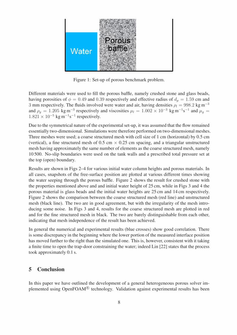
Figure 1: Set-up of porous benchmark problem.

Different materials were used to fill the porous baffle, namely crushed stone and glass beads,

having porosities of φ = 0.49 and 0.39 respectively and effective radius of dp = 1.59 cm and

3 mm respectively. The fluids involved were water and air, having densities ρl = 998.2 kg m−3

and ρg = 1.205 kg m−3 respectively and viscosities µl = 1.002 × 10−3 kg m−1s−1 and µg =1.821× 10−5 kg m−1s−1 respectively.

Due to the symmetrical nature of the experimental set-up, it was assumed that the flow remained

essentially two-dimensional. Simulations were therefore performed on two-dimensional meshes.

Three meshes were used; a coarse structured mesh with cell size of 1 cm (horizontal) by 0.5 cm

(vertical), a fine structured mesh of 0.5 cm × 0.25 cm spacing, and a triangular unstructured

mesh having approximately the same number of elements as the coarse structured mesh, namely

10 500. No-slip boundaries were used on the tank walls and a prescribed total pressure set at

the top (open) boundary.

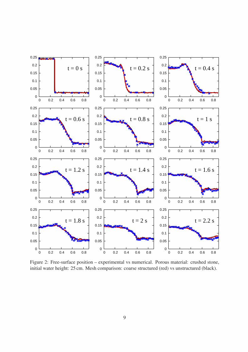
Results are shown in Figs 2–4 for various initial water column heights and porous materials. In

all cases, snapshots of the free-surface position are plotted at various different times showing

the water seeping through the porous baffle. Figure 2 shows the result for crushed stone with

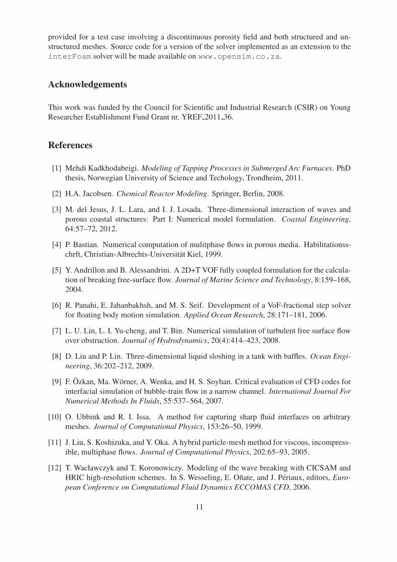
the properties mentioned above and and initial water height of 25 cm, while in Figs 3 and 4 the

porous material is glass beads and the initial water heights are 25 cm and 14 cm respectively.

Figure 2 shows the comparison between the coarse structured mesh (red line) and unstructured

mesh (black line). The two are in good agreement, but with the irregularity of the mesh intro-

ducing some noise. In Figs 3 and 4, results for the coarse structured mesh are plotted in red

and for the fine structured mesh in black. The two are barely distinguishable from each other,

indicating that mesh independence of the result has been achieved.

In general the numerical and experimental results (blue crosses) show good correlation. There

is some discrepancy in the beginning where the lower portion of the measured interface position

has moved further to the right than the simulated one. This is, however, consistent with it taking

a finite time to open the trap-door constraining the water; indeed Lin [22] states that the process

took approximately 0.1 s.

5 Conclusion

In this paper we have outlined the development of a general heterogeneous porous solver im-

plemented using OpenFOAM R© technology. Validation against experimental results has been

8

0

0.05

0.1

0.15

0.2

0.25

0 0.2 0.4 0.6 0.8

t = 0 s

0

0.05

0.1

0.15

0.2

0.25

0 0.2 0.4 0.6 0.8

t = 0.2 s

0

0.05

0.1

0.15

0.2

0.25

0 0.2 0.4 0.6 0.8

t = 0.4 s

0

0.05

0.1

0.15

0.2

0.25

0 0.2 0.4 0.6 0.8

t = 0.6 s

0

0.05

0.1

0.15

0.2

0.25

0 0.2 0.4 0.6 0.8

t = 0.8 s

0

0.05

0.1

0.15

0.2

0.25

0 0.2 0.4 0.6 0.8

t = 1 s

0

0.05

0.1

0.15

0.2

0.25

0 0.2 0.4 0.6 0.8

t = 1.2 s

0

0.05

0.1

0.15

0.2

0.25

0 0.2 0.4 0.6 0.8

t = 1.4 s

0

0.05

0.1

0.15

0.2

0.25

0 0.2 0.4 0.6 0.8

t = 1.6 s

0

0.05

0.1

0.15

0.2

0.25

0 0.2 0.4 0.6 0.8

t = 1.8 s

0

0.05

0.1

0.15

0.2

0.25

0 0.2 0.4 0.6 0.8

t = 2 s

0

0.05

0.1

0.15

0.2

0.25

0 0.2 0.4 0.6 0.8

t = 2.2 s

Figure 2: Free-surface position – experimental vs numerical. Porous material: crushed stone,

initial water height: 25 cm. Mesh comparison: coarse structured (red) vs unstructured (black).

9

0

0.05

0.1

0.15

0.2

0.25

0.3

0 0.2 0.4 0.6 0.8

t = 0 s

0

0.05

0.1

0.15

0.2

0.25

0.3

0 0.2 0.4 0.6 0.8

t = 0.4 s

0

0.05

0.1

0.15

0.2

0.25

0.3

0 0.2 0.4 0.6 0.8

t = 0.8 s

0

0.05

0.1

0.15

0.2

0.25

0.3

0 0.2 0.4 0.6 0.8

t = 1.2 s

0

0.05

0.1

0.15

0.2

0.25

0.3

0 0.2 0.4 0.6 0.8

t = 1.6 s

0

0.05

0.1

0.15

0.2

0.25

0.3

0 0.2 0.4 0.6 0.8

t = 4 s

Figure 3: Free-surface position – experimental vs numerical. Porous material: glass beads,

initial water height 25 cm. Mesh comparison: coarse (red) vs fine (black) structured.

0

0.02

0.04

0.06

0.08

0.1

0.12

0.14

0 0.2 0.4 0.6 0.8

t = 0 s

0

0.02

0.04

0.06

0.08

0.1

0.12

0.14

0 0.2 0.4 0.6 0.8

t = 0.4 s

0

0.02

0.04

0.06

0.08

0.1

0.12

0.14

0 0.2 0.4 0.6 0.8

t = 0.8 s

0

0.02

0.04

0.06

0.08

0.1

0.12

0.14

0 0.2 0.4 0.6 0.8

t = 1.2 s

0

0.02

0.04

0.06

0.08

0.1

0.12

0.14

0 0.2 0.4 0.6 0.8

t = 1.6 s

0

0.02

0.04

0.06

0.08

0.1

0.12

0.14

0 0.2 0.4 0.6 0.8

t = 4 s

Figure 4: Free-surface position – experimental vs numerical. Porous material: glass beads,

initial water height 14 cm. Mesh comparison: coarse (red) vs fine (black) structured.

10

provided for a test case involving a discontinuous porosity field and both structured and un-

structured meshes. Source code for a version of the solver implemented as an extension to the

interFoam solver will be made available on www.opensim.co.za.

Acknowledgements

This work was funded by the Council for Scientific and Industrial Research (CSIR) on Young

Researcher Establishment Fund Grant nr. YREF 2011 36.

References

[1] Mehdi Kadkhodabeigi. Modeling of Tapping Processes in Submerged Arc Furnaces. PhD

thesis, Norwegian University of Science and Techology, Trondheim, 2011.

[2] H.A. Jacobsen. Chemical Reactor Modeling. Springer, Berlin, 2008.

[3] M. del Jesus, J. L. Lara, and I. J. Losada. Three-dimensional interaction of waves and

porous coastal structures: Part I: Numerical model formulation. Coastal Engineering,

64:57–72, 2012.

[4] P. Bastian. Numerical computation of mulitphase flows in porous media. Habilitationss-

chrft, Christian-Albrechts-Universitat Kiel, 1999.

[5] Y. Andrillon and B. Alessandrini. A 2D+T VOF fully coupled formulation for the calcula-

tion of breaking free-surface flow. Journal of Marine Science and Technology, 8:159–168,

2004.

[6] R. Panahi, E. Jahanbakhsh, and M. S. Seif. Development of a VoF-fractional step solver

for floating body motion simulation. Applied Ocean Research, 28:171–181, 2006.

[7] L. U. Lin, L. I. Yu-cheng, and T. Bin. Numerical simulation of turbulent free surface flow

over obstruction. Journal of Hydrodynamics, 20(4):414–423, 2008.

[8] D. Liu and P. Lin. Three-dimensional liquid sloshing in a tank with baffles. Ocean Engi-

neering, 36:202–212, 2009.

[9] F. Ozkan, Ma. Worner, A. Wenka, and H. S. Soyhan. Critical evaluation of CFD codes for

interfacial simulation of bubble-train flow in a narrow channel. International Journal For

Numerical Methods In Fluids, 55:537–564, 2007.

[10] O. Ubbink and R. I. Issa. A method for capturing sharp fluid interfaces on arbitrary

meshes. Journal of Computational Physics, 153:26–50, 1999.

[11] J. Liu, S. Koshizuka, and Y. Oka. A hybrid particle-mesh method for viscous, incompress-

ible, multiphase flows. Journal of Computational Physics, 202:65–93, 2005.

[12] T. Wacławczyk and T. Koronowiczy. Modeling of the wave breaking with CICSAM and

HRIC high-resolution schemes. In S. Wesseling, E. Onate, and J. Periaux, editors, Euro-

pean Conference on Computational Fluid Dynamics ECCOMAS CFD, 2006.

11

[13] I. R. Park, K. S. Kim, J. Kim, and S. H. Van. A volume-of-fluid method for incompressible

free surface flows. International Journal for Numerical Methods in Fluids, 61:1331–1362,

2009.

[14] S. Whitaker. Diffusion and dispersion in porous media. American Institute of Chemical

Engineers Journal, 13:420–427, 1967.

[15] S. Ergun. Fluid flow through packed columns. Chemical Engineering Progress, 48(2):89–

94, 1952.

[16] J. Radestock and R. Jeschar. Theoretische Untersuchung der gegenseitigen Beeinflus-

sung von Temperatur- und Stromungsfeldern in Schuttungen. Chemie Ingenieur Technik,

43(24):1304–1310, 1971.

[17] M.R.A. Van Gent. Formulae to describe porous flow. In Communications on Hydraulic

and Geotechnical Engineering, No. 1992-02, number 92-2, Delft, 1992. Delft University

of Technology.

[18] J. A. Heyns, A. G. Malan, T. M. Harms, and O. F. Oxtoby. Development of a compressive

surface capturing formulation for modelling free-surface flow using the volume-of-fluid

approach. International Journal for Numerical Methods in Fluids, 71:788–804, 2013.

[19] H. Jasak and H. Weller. Interface tracking capabilities of the Inter–Gamma differencing

scheme. Technical report, CFD research group, Imperial College, London, 1995.

[20] C.M. Rhie and W.L. Chow. Numerical study of the turbulent flow past an airfoil with

trailing edge separation. AIAA Journal, 21(11):1525–1532, 1983.

[21] R. I. Issa. Solution of the implicitly discretised fluid flow equations by operator-splitting.

Journal of Computational Physics, 62:40–65, January 1986.

[22] Pengzhi Lin. Numerical modeling of breaking waves. PhD thesis, Cornell University,

1998.

12