A finite volume method for scalar conservation laws with stochastic time–space dependent flux functions

A finite volume method for scalar conservation

laws with stochastic time-space dependent

flux function

Kamel Mohamed a, Mohammed Seaid b, Mostafa Zahri c,∗aDepartment of Computer Science, Faculty of Applied Sciences, University of

Taibah Madinah, KSAbSchool of Engineering and Computing Sciences, University of Durham, South

Road DH1 3LE, UKcDepartment of Mathematics, Faculty of Sciences, University of Taibah, P.O. Box

344 Madinah, KSA

Abstract

We propose a new finite volume method for scalar conservation laws with stochas-tic time-space dependent flux function. The stochastic effects appear in the fluxfunction and can be interpreted as a random manner to localize the discontinuityin the time-space dependent flux function. The location of the interface betweenthe fluxes can be obtained by solving a system of stochastic differential equationsfor the velocity fluctuation and displacement variable. In this paper we develop amodified Rusanov method for the reconstruction of numerical fluxes in the finitevolume discretization. To solve the system of stochastic differential equations forthe interface we apply a second-order Runge-Kutta scheme. Numerical results arepresented for stochastic problems in traffic flow and two-phase flow applications.It is found that the proposed finite volume method offers a robust and accurateapproach for solving scalar conservation laws with stochastic time-space dependentflux functions.

Key words: Conservation laws, Stochastic differential equations, Finite volumemethod, Runge-Kutta scheme, Traffic flow, Buckley-Leverett equation

1 Introduction

Many practical problems in physics and engineering applications are modeledby conservation laws with time-space dependent flux function. These problems

∗ Corresponding author.Email address: [email protected] (Mostafa Zahri).

have been extensively studied in the literature and their numerical solutioncan be accurately computed provided the flux functions, involved coefficients,initial and boundary data are given in a deterministic way. However, mod-eling realistic applications by conservation laws is complicated by the highheterogeneity of the involved coefficients combined with insufficient informa-tion characterizing the flux functions. For instance, in the simulation of trans-port models in ground water flows the exact knowledge of the permeabilityof the soil, the magnitude of source terms, inflow or outflow are usually notknown, see [47] and further references are therein. Another example concernsthe traffic flow in multi-lane roads where the behavior of drivers may turn torandom in making the decision in which lane should the car be, see for example[46,3]. Other applications include multi-phase flow problems [18] conservationlaws in networks [40] and production in supply chains [5]. For supply chains,the uncertainty is included in the processors as random breakdowns and ran-dom repair times. Under these circumstances the probabilistic aspects of theproblem under consideration need to be taken into account for a realistic sim-ulation of its numerical solution. The uncertainties mentioned above can beconveniently described by random fields, whose statistics are usually inferredfrom experiments. This requires to include, in the conservation laws modelingthe problem at hands, a rational assessment of uncertainty, we refer the readerto [7,32,13,14,16] for more details on the uncertainty quantification in conser-vation laws. Consequently, this leads to the notion of scalar conservation lawswith stochastic time-space dependent flux function. For the problems consid-ered in this study, a stochastic differential system, for the velocity fluctuationand the displacement, is used to quantify uncertainties in the conservationlaws. More precisely, the location of the discontinuity in the flux function isassumed to be driven by a drift towards the expected value and a stochas-tic noise term governed by the derivative of a Wiener process. In comparisonwith the deterministic conservation laws with discontinuous flux function, theappearance of the noise in the location of the interface can be seen as the in-tegral effect of microscopic interactions, which produce a continuous sequenceof small and almost stochastic velocity and location changes.A number of numerical methods have been developed to solve stochastic par-tial differential equations. The obvious methods widely used in the literatureare the Monte-Carlo algorithms. These methods generate a sequence of inde-pendent realizations of the solution by sampling the coefficients involved inthe problem under consideration and solving the resulting deterministic partialdifferential equations using standard numerical tools. The obtained solutionsare used to compute statistical characteristics of the solution in the problem,see [20] among others. However, Monte-Carlo algorithms are known to be com-putationally expensive and are only recommended as the last resort. Anothermethod widely used in computational fluid dynamics is the Wiener chaos ex-pansions, see for example [9,19]. In this approach, random fields are discretizedusing polynomial chaos resulting in a set of coupled deterministic partial dif-ferential equations to be solved for each chaos coefficient. However, the Wiener

2

chaos expansions have some limitations in application to the conservation lawswith complex stochastic flux functions. For instance, large number of chaoscoefficients in the expansions are needed to accurately compute small scales. Inaddition, many realizations have to be performed to obtain accurate estimatesof the required statistical characteristics. Therefore, Wiener chaos expansionsare computationally expensive. On the other hand, solving stochastic partialdifferential equations using properties of Wick calculus was also discussed, forinstance in [17,29]. The main idea of this approach is to use properties ofthe Wick product along with the Hermite polynomials to decompose solutionvariables using an orthogonal basis and solve series of uncoupled determin-istic equations. However, the treatment of nonlinear stochastic conservationlaws in these methods is not trivial and high-order statistical moments arenot easy to compute. The concept of incorporating uncertainty in linear hy-perbolic equations of conservation laws is not new, see for example [49,43,11].The mathematical equations studied in these references consist of the modelscalar wave equation with random wave speed subject to given truncatedKarhunen-Loeve expansions. In addition, the numerical techniques presentedin these references are essentially based on a spectral representation in randomspace that exhibits fast convergence only when the solution depends smoothlyon the involved random parameters. On the other hand, there are severalwell-established techniques for modeling stochastic effects such as Galerkinprojection, chaos polynomials, and collocation methods among others. Re-cently, the trend has focused on the development of numerical methods whichmodel nonlinear hyperbolic systems of conservation laws. These include theincorporation of stochastic perturbations into the forcing terms [4], and theincorporation of stochastic variables into the physical flux functions [45,32].The latter method has recently been extended by using adaptive anisotropicspectral procedures [44], such that the stochastic resolution level is based onthe local smoothness of the solution in the stochastic domain. For the con-struction of numerical fluxes, the authors in [45,32,44] consider the Roe-typemethod which may become computationally expensive for hyperbolic systemsof conservation laws with source terms and it may also require entropy cor-rection to accurately capture shocks. Furthermore, truncation techniques inthe polynomial chaos expansions may result in non-physical solutions such asnegative second-order statistical moments. So the method of polynomial chaosexpansions can be applied only for limited applications in nonlinear conserva-tion laws. In the current work, we are interested in scalar conservation laws forwhich the physical flux function switches from one form to another dependingon a random location in the spatial domain. This allows the flux function inthe conservation laws under study to vary in the space and random variables.The location and speed of the discontinuity in the flux function are resolvedby solving an extra system of stochastic ordinary differential equations.The aim of the present work is to implement a robust algorithm for solvingscalar conservation laws with stochastic time-space dependent flux function.The key idea consists on combining a finite volume method for the spatial

3

discretization with a second-order explicit stochastic Runge-Kutta scheme de-veloped in [35–37] for the time integration of the stochastic differential equa-tions. The emphasis in this study is given to a modified Rusanov methodstudied and analyzed in [30] for the spatial discretization. This method is sim-ple, accurate and avoids the solution of Riemann problems during the timeintegration process. The combined method is linearly stable provided the con-dition for the canonical Courant-Friedrichs-Lewy (CFL) condition is satisfied.Our main goal is to present a class of numerical methods that are simple, easyto implement, and accurately solves the stochastic conservation laws withoutrelying on a Riemann solver or direct statistical algorithms. We should men-tion that the finite volume method presented in this paper also differs fromthe traditional Rusanov approach [38] in the fact that the characteristic speedis assumed to be constant, whereas in the present work we use an adaptiveselection of the characteristic speed based on the location of shocks withinthe computational domain. To the best of our knowledge, this is the first timethat a finite volume method is used to solve stochastic equations of nonlinearconservation laws with discontinuous time-space dependent flux functions.

Numerical results are illustrated for several test examples on scalar conserva-tion laws with stochastic time-space dependent flux function. In the first case,analytical solution is available and thus it can be used for verification of con-vergence rates and accuracy of the proposed numerical schemes. In the othercases, comparison to deterministic solutions is presented to illustrate stochasticeffects. Our method accurately approximates the numerical solution to thesenonlinear problems. The obtained results demonstrate good shock resolutionwith high accuracy in smooth regions and without any nonphysical oscillationsnear the shock areas or extensive numerical dissipation. The performance ofthe developed solvers is very attractive since the computed solutions remainstable, monotone and highly accurate without solving Riemann problems orusing demanding computational resources.

The rest of this paper is organized as follows. In section 2 we introduce theequations for scalar conservation laws with stochastic time-space dependentflux function. The finite volume method for stochastic conservation laws isformulated in section 3. This section also includes the time integration of thestochastic differential equations for the interface and the reconstruction of thenumerical fluxes in the finite volume discretization. In section 4 we presentnumerical results for several test examples. Section 5 summarizes the paperwith concluding remarks.

2 Stochastic conservation laws

Let (Ω,F ,P) be a probability space, where Ω is the space of basic outcomes,F is the σ-algebra associated with Ω, and P is the (probability) measure onF . This σ-algebra can be interpreted as a collection of all possible events thatcould be derived from the basic outcomes in Ω, and that have a probability

4

that is well defined with respect to P. A random variable X is a mappingX : Ω −→ R. The Lp-norm of a random variable can be defined as

‖X‖p = 〈|X|p〉1/p , for 0 < p <∞,

where 〈·〉 denotes the operation of mathematical expectation. Equipped withthis norm, the space Lp is a Banach space of all random variables X definedon (Ω,F ,P) and having a finite norm. In the current study, we are interestedin developing robust numerical methods for approximating solutions of theCauchy problem associated with the following stochastic scalar conservationlaws

∂u

∂t+

∂

∂xF (X, u)= 0, (x, t) ∈ R× (t0, T ],

(1)u(t0, x)=u0(x), x ∈ R,

where (t0, T ] is the time interval, u ∈ R is the scalar unknown, the flux functionF (X, u) : Ω × R −→ R is nonlinear, u0(x) is an initial condition given attime t0, and X is a stochastic process that can depend on space or/and timevariable as well. In the deterministic case (with X = k(x)), the multiplicativeflux function

F (k(x), u) = k(x)G(u), k(x) =

kL, if x < 0,

kR, if x > 0,(2)

has been widely used in the literature for theoretical and numerical analysisof conservation laws with discontinuous flux function. In (2), G(u) is a con-tinuous flux function in R, kl and kR are positive constants with kL 6= kR.In all cases, we assume that the Jacobian F ′(k(x), u) = ∂F (k(x), u)/∂u isdiagonalizable with real eigenvalues. It should be noted that hyperbolic equa-tions of conservation laws with discontinuous flux function of type (2) occur inmany physical applications, for example in transport models in porous media[10], sedimentation phenomena [6], resonant models [21] and vehicular trafficflows [28,15]. Most practical applications of these problems cannot be solvedanalytically and hence require numerical methods. One of the main difficultiesin the analysis of problem (1)-(2) is the correct definition of a solution. It iswell known that after a finite time the problem (1)-(2) does not in generalpossess a continuous solution even if the initial data u0 is sufficiently smooth.Hence a solution of (1)-(2) has to be understood in the weak sense. Moreover,among the difficulties that arose when approximating solutions of (1)-(2) arenumerical instability, poor shock and rarefaction resolutions, and even spuri-ous numerical solutions, see for instance [1,25,39] and references are therein.

Our objective in this paper is to develop an efficient numerical method for solv-ing the stochastic scalar conservation laws (1) equipped with a discontinuous

5

flux function of the form

F (X, u) =(1−HX (x)

)f(u) +HX (x) g(u), (3)

where f and g are continuous flux functions, andHX (x) is a Heaviside functiondefined as

HX (x) =

1, if P (x < X) = 1,

0, if P (x > X) = 1.(4)

Here, the stochastic process X can be seen as a random interface separatingtwo media with different physical properties. The location of this interfacemay be moving within the spatial domain and time interval according to theprobability P. Examples of recent applications in stochastic interface modelscan be found in [2] for growing interfaces in quenched media, in [24] for com-posite materials with stochastic interface defects, in [8] for dynamics of iontransfer across liquid-liquid interfaces, and in [48] for random elliptic interfaceproblems. The common practice in stochastic interface models is to analyzethe kinetics obtained from transition-state theory independently from stochas-tic molecular dynamic simulations. In general, the interface equations derivedfrom the microscopic rules using regularization procedure predict accuratelythe roughness. The main contribution of the present work is to present an ef-ficient finite volume method for solving conservation laws with discontinuousflux functions subject to the stochastic interface equation (4). Note that bysetting X = 0 and changing the stochastic function HX (x) in (3) to the stan-dard Heaviside function, one recover the classical equations for deterministicconservation laws with discontinuous flux functions

F (u) =

f(u), if x < 0,

g(u), if x > 0.(5)

This class of problems has been widely studied in the literature, see for ex-ample [1,25,39]. The considered conservation laws involve stochastic effect,which increases the difficulty for solving them. This makes the developmentof numerical methods for stochastic conservation laws more attractive.

To close the system of equations (1) and (3) an equation describing the evo-lution of X is required. In the current work, the equations prescribing theevolution of the velocity fluctuation V and the displacement X are solutionsof the following system of stochastic differential equation (SDE)

dV = a (X,V ) dt+ b (t) dW, V (t0) = V0,(6)

dX =V dt+ εdW, X(t0) = X0,

where a (X,V ) is a given drift function, b (t) is a given diffusion function, Wis a Wiener process, X0 and V0 are known initial conditions at time t0, and

6

ε is a constant characterizing the rate of dissipation in the SDE. Note thatin the system (6), the two terms in the right-hand side of each equation mayrepresent the effects of the turbulent flow on the solution and they dependon the Lagrangian time scale and the velocity fluctuation standard deviation.In practice, the drift term a (X,V ) refers to fluctuations caused by the largescales, whereas the diffusion term b (t) is related to short term fluctuations.

The new model (6) presented in this paper to detect the interface in theconservation laws (1) is similar to the stochastic model for molecular motionin fluid dynamic equations. In these models, the kinetic fluid equations aresolved through the stochastic motion of particles

dVidt

=−1

τ(Vi − Ui) +

√4es3τ

dWi

dt,

(7)dXi

dt=Vi,

where Xi is the position of the ith particle, Vi is the molecular velocity of theparticle, τ is the relaxation time, es is the sensible energy of the fluid andUi is its mean velocity, compare [23] among others. Here, at the microscopicscale, the equations (7) represent statistical moments of the particle ensemblein the particle location X at time t. The mean velocity U is equivalent to thefluid velocity measured on the macroscopic fluid dynamic scale according tothe ergodic theorem [12]. Note that the conservation law (1) and the interfaceequation (6) are not fully coupled such that once the SDE (6) is solved for theinterface X, the flux function F (X, u) is updated using (3) and then used inthe numerical solution of the conservation laws (1). A possible fully coupledversion of the model consists on solving the following system of stochasticdifferential equations

du=−(∂

∂xF (X, u)

)dt+ σ (t, x) dW, u(t0) = u0,

dV = a (X,V ) dt+ b (t) dW, V (t0) = V0, (8)

dX =V dt+ εdW, X(t0) = X0,

where σ is the amplitude of the random noise to be defined accordingly. How-ever, the drawback of considering the coupled system (8) lies on the hugeamount of computational cost needed for its time and space discretizationsand also on the two-scale aspect of the problem. Remark that, in general ap-plications, the time scale for the first equation in (8) is far different from thetime scale in the two other equations. This may require an unacceptably smalltime steps to accurately capture the dynamics of the numerical solutions.

It should be stressed that the numerical techniques presented in this papercan be extended, without major conceptual modifications, to the generalized

7

stochastic conservation laws (1) with a flux function defined as

F(X(1), . . . , X(N), u

)= HX(1)f1(u) + · · ·+HX(N)fN(u), (9)

where fk(u), with k = 1, . . . , N are continuous flux functions, and HX(k) (x)are Heaviside-type functions defined as

HX(k) (x) =

1, if P

(x < X(k)

)= 1,

0, if P(x > X(k)

)= 1,

(10)

and satisfy the condition

HX(1) (x) +HX(2) (x) + · · ·+HX(N) (x) = 1.

Note that X(k), with k = 1, . . . , N can be seen as stochastic locations of thediscontinuities in the flux function (9). As in the one-dimensional SDE (6),

V =(V (1), . . . , V (N)

)Tand X =

(X(1), . . . , X(N)

)Trepresent respectively, the

N -vector of velocity fluctuations and stochastic processes solving the followingsystem of stochastic differential equations

dV=A (X,V) dt+ B (t) dW, V(t0) = V0,(11)

dX=Vdt+ εdW, X(t0) = X0,

where A (X,V) is the drift N -vector, B (t) is the diffusion N×d-matrix, W isa d-vector Wiener process, X0 and V0 are known N -vector of initial conditionsgiven at time t0. Here, each entry of the d-vector W forms a Brownian motionwhich is independent of the other elements.

It is worth pointing out that in general, it is difficult to derive an effectiveequation to be solved for the the average solution. However, for a fixed velocitythe interface motion is governed by the SDE

dX = V dt+ εdW, (12)

where the position X(t) process is Markovian and the evolution of its prob-ability density function p(t, x), is described by an advection-diffusion type ofpartial differential equation known as the Fokker-Planck equation [22]

∂p

∂t+

∂

∂x(V p)− 1

2

∂2

∂x2

(ε2p)= 0. (13)

The initial spreading of a cloud of particles is very small and its distributioncan be modelled using a Dirac delta function as

p(0, x) = δ (x− x0) .

8

By assuming a zero diffusion and divergence-free velocity the equation (13)reduces to the advection equation for the interface φ

∂φ

∂t+ V

∂φ

∂x= 0, (14)

that is similar to the interface equation widely used in level set methods (seefor example [31]) in the sense that it replaces the microscopic model by asimpler model, namely Fokker-Planck model, but due to the implementationas particle method no discretization of the distribution function is necessary.Indeed, by interpreting the Fokker-Planck equation (13) as an advection equa-tion makes the stochastic model in (6) to be consistent with the well-knowninterfacial flows used in the computational fluids dynamics.

3 Finite volume method for the stochastic conservation laws

Finite volume methods are preferable in numerical solutions of partial dif-ferential equations of hyperbolic type due to their conservation properties.These techniques have been developed mainly under assumptions of ideal in-put such as deterministic flux functions, initial data and computational do-main. In practice, this is hardly the case as the flux functions and the inputdata involve uncertainties. In the current study, we propose a new finite vol-ume method for stochastic conservation laws (1). To formulate our method,we discretize the spatial domain into control volumes [xi−1/2, xi+1/2] with uni-form size ∆x = xi+1/2 − xi−1/2 for simplicity. We also divide the time interval[t0, T ] into subintervals [tn, tn+1] with uniform size ∆t. Following the standardfinite volume formulation, we integrate the considered equation (1) with re-spect to time and space over the domain [tn, tn+1] × [xi−1/2, xi+1/2] to obtainthe following discrete equation

Un+1i = Un

i − ∆t

∆x

(F(Xn+1, Un

i+1/2

)− F

(Xn+1, Un

i−1/2

)), (15)

where Xn+1 denotes an approximation of the stochastic process X at timetn+1, U

ni±1/2 = u(tn, xi±1/2), U

ni is the space average of the solution u in the

domain [xi−1/2, xi+1/2] at time tn i.e.,

Uni =

1

∆t∆x

∫ tn+1

tn

∫ xi+1/2

xi−1/2

u(t, x) dt dx,

and F (Xn+1, Uni±1/2) is the numerical flux at x = xi±1/2 and time tn. The

spatial discretization of the equation (15) is complete when a numerical ap-proximation of Xn+1 is computed by solving the SDE (6) and a construction ofthe numerical fluxes F (Xn+1, Un

i±1/2) is chosen. In what follows we discuss theformulation of a modified Rusanov method for the numerical approximationof the fluxes and we also formulate a stochastic Runge-Kutta scheme for thenumerical solution of the system of stochastic differential equations.

9

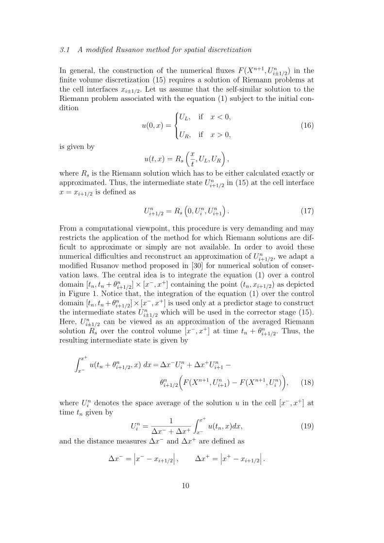
3.1 A modified Rusanov method for spatial discretization

In general, the construction of the numerical fluxes F (Xn+1, Uni±1/2) in the

finite volume discretization (15) requires a solution of Riemann problems atthe cell interfaces xi±1/2. Let us assume that the self-similar solution to theRiemann problem associated with the equation (1) subject to the initial con-dition

u(0, x) =

UL, if x < 0,

UR, if x > 0,(16)

is given by

u(t, x) = Rs

(x

t, UL, UR

),

where Rs is the Riemann solution which has to be either calculated exactly orapproximated. Thus, the intermediate state Un

i+1/2 in (15) at the cell interfacex = xi+1/2 is defined as

Uni+1/2 = Rs

(0, Un

i , Uni+1

). (17)

From a computational viewpoint, this procedure is very demanding and mayrestricts the application of the method for which Riemann solutions are dif-ficult to approximate or simply are not available. In order to avoid thesenumerical difficulties and reconstruct an approximation of Un

i+1/2, we adapt amodified Rusanov method proposed in [30] for numerical solution of conser-vation laws. The central idea is to integrate the equation (1) over a controldomain [tn, tn + θni+1/2]× [x−, x+] containing the point (tn, xi+1/2) as depictedin Figure 1. Notice that, the integration of the equation (1) over the controldomain [tn, tn+ θ

ni+1/2]× [x−, x+] is used only at a predictor stage to construct

the intermediate states Uni±1/2 which will be used in the corrector stage (15).

Here, Uni±1/2 can be viewed as an approximation of the averaged Riemann

solution Rs over the control volume [x−, x+] at time tn + θni+1/2. Thus, theresulting intermediate state is given by

∫ x+

x−u(tn + θni+1/2, x) dx=∆x−Un

i +∆x+Uni+1 −

θni+1/2

(F (Xn+1, Un

i+1)− F (Xn+1, Uni )), (18)

where Uni denotes the space average of the solution u in the cell [x−, x+] at

time tn given by

Uni =

1

∆x− +∆x+

∫ x+

x−u(tn, x)dx, (19)

and the distance measures ∆x− and ∆x+ are defined as

∆x− =∣∣∣x− − xi+1/2

∣∣∣ , ∆x+ =∣∣∣x+ − xi+1/2

∣∣∣ .10

+i+1/2n xxxxt

θ+ntn

θ+nt

t

∆ ∆x x+

U Ui+1i

i+1/2

i+1/2

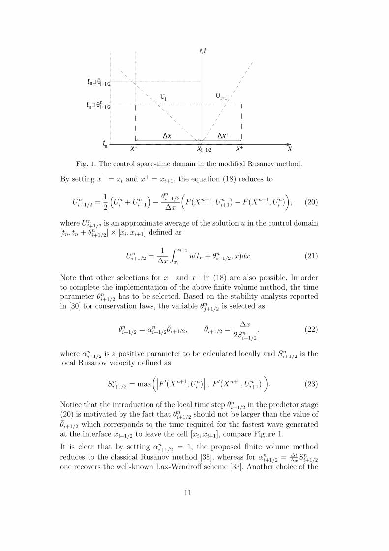
Fig. 1. The control space-time domain in the modified Rusanov method.

By setting x− = xi and x+ = xi+1, the equation (18) reduces to

Uni+1/2 =

1

2

(Uni + Un

i+1

)−θni+1/2

∆x

(F (Xn+1, Un

i+1)− F (Xn+1, Uni )), (20)

where Uni+1/2 is an approximate average of the solution u in the control domain

[tn, tn + θni+1/2]× [xi, xi+1] defined as

Uni+1/2 =

1

∆x

∫ xi+1

xiu(tn + θni+1/2, x)dx. (21)

Note that other selections for x− and x+ in (18) are also possible. In orderto complete the implementation of the above finite volume method, the timeparameter θni+1/2 has to be selected. Based on the stability analysis reportedin [30] for conservation laws, the variable θnj+1/2 is selected as

θni+1/2 = αni+1/2θi+1/2, θi+1/2 =∆x

2Sni+1/2

, (22)

where αni+1/2 is a positive parameter to be calculated locally and Sni+1/2 is thelocal Rusanov velocity defined as

Sni+1/2 = max(∣∣∣F ′(Xn+1, Un

i )∣∣∣ , ∣∣∣F ′(Xn+1, Un

i+1)∣∣∣). (23)

Notice that the introduction of the local time step θni+1/2 in the predictor stage(20) is motivated by the fact that θni+1/2 should not be larger than the value of

θi+1/2 which corresponds to the time required for the fastest wave generatedat the interface xi+1/2 to leave the cell [xi, xi+1], compare Figure 1.

It is clear that by setting αni+1/2 = 1, the proposed finite volume method

reduces to the classical Rusanov method [38], whereas for αni+1/2 = ∆t∆xSni+1/2

one recovers the well-known Lax-Wendroff scheme [33]. Another choice of the

11

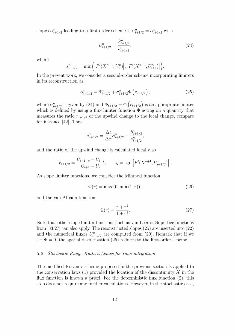
slopes αni+1/2 leading to a first-order scheme is αni+1/2 = αni+1/2 with

αni+1/2 =Sni+1/2

sni+1/2

, (24)

where

sni+1/2 = min(∣∣∣F ′(Xn+1, Un

i )∣∣∣ , ∣∣∣F ′(Xn+1, Un

i+1)∣∣∣).

In the present work, we consider a second-order scheme incorporating limitersin its reconstruction as

αni+1/2 = αni+1/2 + σni+1/2Φ(ri+1/2

), (25)

where αni+1/2 is given by (24) and Φi+1/2 = Φ(ri+1/2

)is an appropriate limiter

which is defined by using a flux limiter function Φ acting on a quantity thatmeasures the ratio ri+1/2 of the upwind change to the local change, comparefor instance [42]. Thus,

σni+1/2 =∆t

∆xSni+1/2 −

Sni+1/2

sni+1/2

,

and the ratio of the upwind change is calculated locally as

ri+1/2 =Ui+1−q − Ui−qUi+1 − Ui

, q = sgn[F ′(Xn+1, Un

i+1/2)].

As slope limiter functions, we consider the Minmod function

Φ(r) = max (0,min (1, r)) , (26)

and the van Albada function

Φ(r) =r + r2

1 + r2. (27)

Note that other slope limiter functions such as van Leer or Superbee functionsfrom [33,27] can also apply. The reconstructed slopes (25) are inserted into (22)and the numerical fluxes Un

i+1/2 are computed from (20). Remark that if weset Φ = 0, the spatial discretization (25) reduces to the first-order scheme.

3.2 Stochastic Runge-Kutta schemes for time integration

The modified Rusanov scheme proposed in the previous section is applied tothe conservation laws (1) provided the location of the discontinuity X in theflux function is known a priori. For the deterministic flux function (2), thisstep does not require any further calculations. However, in the stochastic case,

12

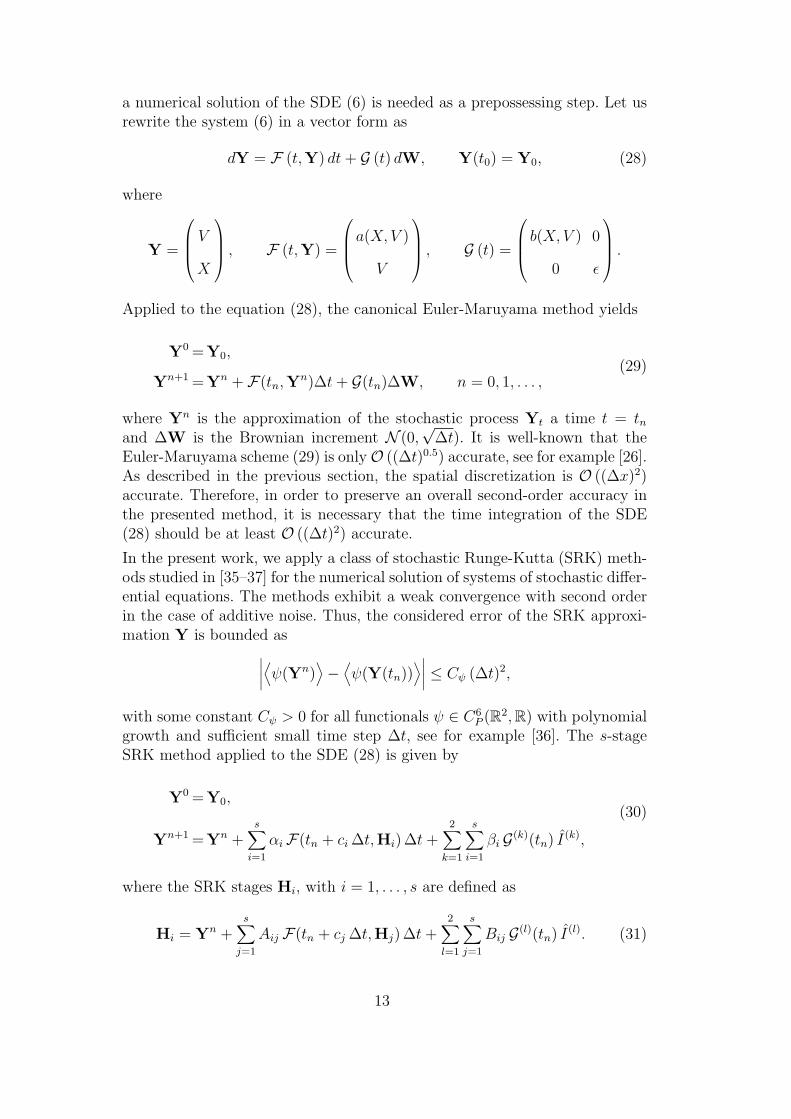
a numerical solution of the SDE (6) is needed as a prepossessing step. Let usrewrite the system (6) in a vector form as

dY = F (t,Y) dt+ G (t) dW, Y(t0) = Y0, (28)

where

Y =

VX

, F (t,Y) =

a(X,V )

V

, G (t) =

b(X,V ) 0

0 ε

.Applied to the equation (28), the canonical Euler-Maruyama method yields

Y0 =Y0,(29)

Yn+1 =Yn + F(tn,Yn)∆t+ G(tn)∆W, n = 0, 1, . . . ,

where Yn is the approximation of the stochastic process Yt a time t = tnand ∆W is the Brownian increment N (0,

√∆t). It is well-known that the

Euler-Maruyama scheme (29) is onlyO ((∆t)0.5) accurate, see for example [26].As described in the previous section, the spatial discretization is O ((∆x)2)accurate. Therefore, in order to preserve an overall second-order accuracy inthe presented method, it is necessary that the time integration of the SDE(28) should be at least O ((∆t)2) accurate.

In the present work, we apply a class of stochastic Runge-Kutta (SRK) meth-ods studied in [35–37] for the numerical solution of systems of stochastic differ-ential equations. The methods exhibit a weak convergence with second orderin the case of additive noise. Thus, the considered error of the SRK approxi-mation Y is bounded as∣∣∣∣⟨ψ(Yn)

⟩−⟨ψ(Y(tn))

⟩∣∣∣∣ ≤ Cψ (∆t)2,

with some constant Cψ > 0 for all functionals ψ ∈ C6P (R2,R) with polynomial

growth and sufficient small time step ∆t, see for example [36]. The s-stageSRK method applied to the SDE (28) is given by

Y0 =Y0,(30)

Yn+1 =Yn +s∑i=1

αiF(tn + ci∆t,Hi)∆t+2∑

k=1

s∑i=1

βi G(k)(tn) I(k),

where the SRK stages Hi, with i = 1, . . . , s are defined as

Hi = Yn +s∑j=1

Aij F(tn + cj ∆t,Hj)∆t+2∑l=1

s∑j=1

Bij G(l)(tn) I(l). (31)

13

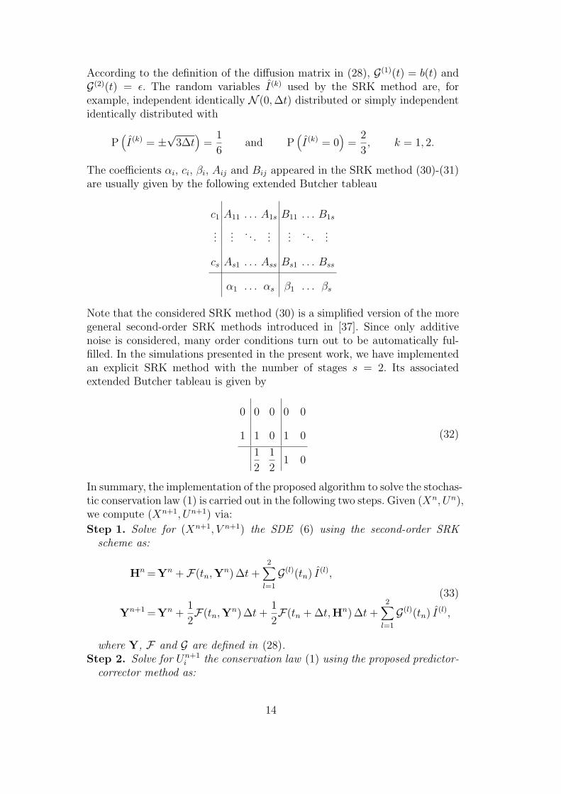
According to the definition of the diffusion matrix in (28), G(1)(t) = b(t) andG(2)(t) = ε. The random variables I(k) used by the SRK method are, forexample, independent identically N (0,∆t) distributed or simply independentidentically distributed with

P(I(k) = ±

√3∆t

)=

1

6and P

(I(k) = 0

)=

2

3, k = 1, 2.

The coefficients αi, ci, βi, Aij and Bij appeared in the SRK method (30)-(31)are usually given by the following extended Butcher tableau

c1 A11 . . . A1s B11 . . . B1s

......

. . ....

.... . .

...

cs As1 . . . Ass Bs1 . . . Bss

α1 . . . αs β1 . . . βs

Note that the considered SRK method (30) is a simplified version of the moregeneral second-order SRK methods introduced in [37]. Since only additivenoise is considered, many order conditions turn out to be automatically ful-filled. In the simulations presented in the present work, we have implementedan explicit SRK method with the number of stages s = 2. Its associatedextended Butcher tableau is given by

0 0 0 0 0

1 1 0 1 0

1

2

1

21 0

(32)

In summary, the implementation of the proposed algorithm to solve the stochas-tic conservation law (1) is carried out in the following two steps. Given (Xn, Un),we compute (Xn+1, Un+1) via:

Step 1. Solve for (Xn+1, V n+1) the SDE (6) using the second-order SRKscheme as:

Hn=Yn + F(tn,Yn)∆t+

2∑l=1

G(l)(tn) I(l),

(33)

Yn+1 =Yn +1

2F(tn,Y

n)∆t+1

2F(tn +∆t,Hn)∆t+

2∑l=1

G(l)(tn) I(l),

where Y, F and G are defined in (28).Step 2. Solve for Un+1

i the conservation law (1) using the proposed predictor-corrector method as:

14

Uni+1/2 =

1

2

(Uni + Un

i+1

)−

αni+1/2

2Sni+1/2

(F (Xn+1, Un

i+1)− F (Xn+1, Uni )),

(34)

Un+1i =Un

i − ∆t

∆x

(F(Xn+1, Un

i+1/2

)− F

(Xn+1, Un

i−1/2

)),

where Sni+1/2 and αni+1/2 are defined in (23) and (25), respectively.

It is evident that, due to the stochasticity in the conservation law (1), the abovealgorithm is used to generate a numberM of realizations. Thus, a Monte Carlosimulation is performed for the solution samples Un

m for m = 1, . . . ,M , andwe estimate the expectation of the solution Un+1 at time tn+1 by

〈ψ(Un+1)〉 ≈ 1

M

M∑m=1

ψ(Un+1m

).

Note that other SRK methods from [37] can also be applied for solving theSDE system (28).

4 Numerical results

We present numerical results for several test problems to check the accuracyand the performance of the proposed finite volume method. As with all ex-plicit time stepping methods the theoretical maximum stable time step ∆t isspecified according to the CFL condition

∆t = Cr∆x

maxi

(∣∣∣αni+1/2Sni+1/2

∣∣∣) , (35)

where Cr is a constant to be chosen less than unity. In all our simulations,the fixed Courant number Cr = 0.75 is used and the time step is variedaccording to (35). In all the simulations (unless stated) we performM = 1000realizations and mean solutions are displayed. The following test examples areselected:

4.1 Accuracy test problems

Our first example is a deterministic conservation law with exact steady-statesolution which can be used to quantify the results obtained by the classicalRusanov method and the proposed modified Rusanov method. This examplecan also serve to test the ability of the above finite volume method to con-verge to the correct entropy solution. The problem statement is given by the

15

equations (1)-(2) where

G(u) = u(1− u), k(x) =

2, if 0 ≤ x ≤ 2.5,

25−2x10

, if 2.5 < x < 7.5,

1, if 7.5 ≤ x ≤ 10,

(36)

and an initial condition given by

u0(x) =

0.9, if 0 ≤ x ≤ 2.5,

1+√0.282

, if 2.5 < x ≤ 10.

This problem has a steady exact solution given by

u∞(x) =

0.9, if 0 ≤ x ≤ 2.5,

12+

√k(x)2−0.72k(x)

2k(x), if 2.5 < x < 7.5,

1+√0.282

, if 7.5 ≤ x ≤ 10.

We compute the approximate solution at time t = 20. At this time the ap-proximated solutions are almost stationary, and therefore error norms can becalculated. We consider the L∞-, L1- and L2-error norms defined as

max1≤i≤N

|Ui − u∞(xi)| ,N∑i=1

|Ui − u∞(xi)|∆x,

√√√√ N∑i=1

|Ui − u∞(xi)|2 ∆x,

respectively. Here, Ui and u∞(xi) are respectively, the computed and exactsteady-state solutions at gridpoint xi, whereas N stands for the number ofgridpoints used in the spatial discretization. The obtained results for the clas-sical Rusanov method are listed in Table 1 along with their correspondingconvergence rates. Those corresponding to the proposed modified Rusanovmethod using the van Albada limiter are presented in Table 2. It reveals thatincreasing the number of gridpoints in the computational domain results in adecay of all considered error norms in both methods. The results provided bythe modified Rusanov method are more accurate than the results provided bythe classical Rusanov method. Our modified Rusanov method exhibits goodconvergence behavior for this nonlinear problem. As can be seen from the con-vergence rates presented in these tables, the classical Rusanov method showsonly a first-order accuracy, whereas a second-order accuracy is achieved in ourmethod for this test example in terms of the considered error norms. A similartrend has been observed in the errors (not reported here) obtained using theMinMod limiter in the proposed modified Rusanov method.

Next we examine the accuracy of the considered SRK scheme for solvingstochastic differential equations. To this end we solve the linear stochastic

16

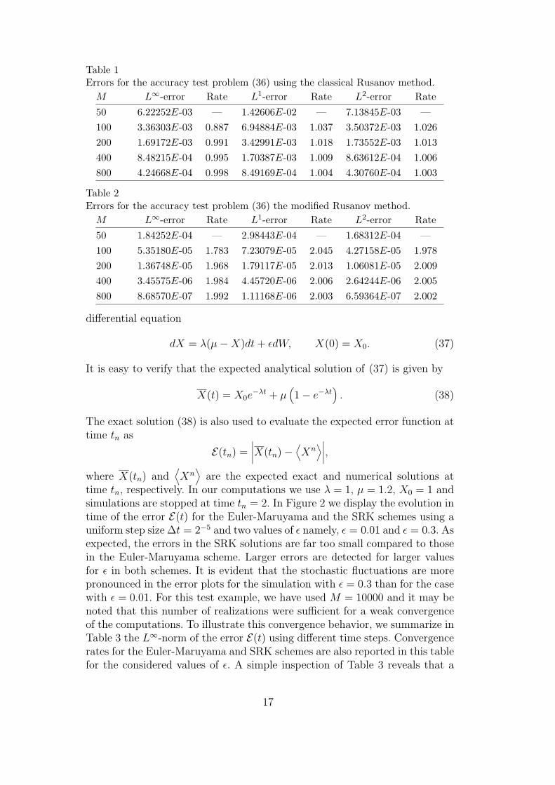
Table 1Errors for the accuracy test problem (36) using the classical Rusanov method.

M L∞-error Rate L1-error Rate L2-error Rate

50 6.22252E-03 — 1.42606E-02 — 7.13845E-03 —

100 3.36303E-03 0.887 6.94884E-03 1.037 3.50372E-03 1.026

200 1.69172E-03 0.991 3.42991E-03 1.018 1.73552E-03 1.013

400 8.48215E-04 0.995 1.70387E-03 1.009 8.63612E-04 1.006

800 4.24668E-04 0.998 8.49169E-04 1.004 4.30760E-04 1.003

Table 2Errors for the accuracy test problem (36) the modified Rusanov method.

M L∞-error Rate L1-error Rate L2-error Rate

50 1.84252E-04 — 2.98443E-04 — 1.68312E-04 —

100 5.35180E-05 1.783 7.23079E-05 2.045 4.27158E-05 1.978

200 1.36748E-05 1.968 1.79117E-05 2.013 1.06081E-05 2.009

400 3.45575E-06 1.984 4.45720E-06 2.006 2.64244E-06 2.005

800 8.68570E-07 1.992 1.11168E-06 2.003 6.59364E-07 2.002

differential equation

dX = λ(µ−X)dt+ εdW, X(0) = X0. (37)

It is easy to verify that the expected analytical solution of (37) is given by

X(t) = X0e−λt + µ

(1− e−λt

). (38)

The exact solution (38) is also used to evaluate the expected error function attime tn as

E(tn) =∣∣∣∣X(tn)−

⟨Xn

⟩∣∣∣∣,where X(tn) and

⟨Xn

⟩are the expected exact and numerical solutions at

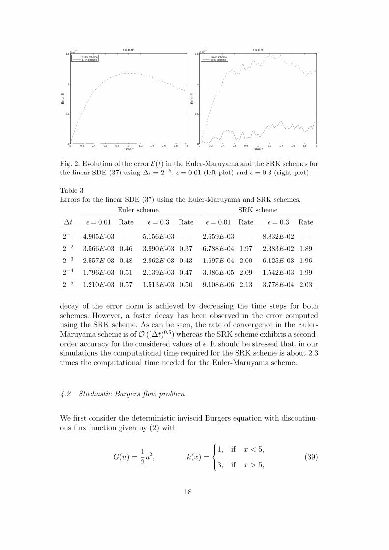
time tn, respectively. In our computations we use λ = 1, µ = 1.2, X0 = 1 andsimulations are stopped at time tn = 2. In Figure 2 we display the evolution intime of the error E(t) for the Euler-Maruyama and the SRK schemes using auniform step size ∆t = 2−5 and two values of ε namely, ε = 0.01 and ε = 0.3. Asexpected, the errors in the SRK solutions are far too small compared to thosein the Euler-Maruyama scheme. Larger errors are detected for larger valuesfor ε in both schemes. It is evident that the stochastic fluctuations are morepronounced in the error plots for the simulation with ε = 0.3 than for the casewith ε = 0.01. For this test example, we have used M = 10000 and it may benoted that this number of realizations were sufficient for a weak convergenceof the computations. To illustrate this convergence behavior, we summarize inTable 3 the L∞-norm of the error E(t) using different time steps. Convergencerates for the Euler-Maruyama and SRK schemes are also reported in this tablefor the considered values of ε. A simple inspection of Table 3 reveals that a

17

0 0.2 0.4 0.6 0.8 1 1.2 1.4 1.6 1.8 20

0.5

1

1.5x 10

−3

Time t

Err

or E

ε = 0.01

Euler schemeSRK scheme

0 0.2 0.4 0.6 0.8 1 1.2 1.4 1.6 1.8 20

0.5

1

1.5x 10

−3

Time t

Err

or E

ε = 0.3

Euler schemeSRK scheme

Fig. 2. Evolution of the error E(t) in the Euler-Maruyama and the SRK schemes forthe linear SDE (37) using ∆t = 2−5. ε = 0.01 (left plot) and ε = 0.3 (right plot).

Table 3Errors for the linear SDE (37) using the Euler-Maruyama and SRK schemes.

Euler scheme SRK scheme

∆t ε = 0.01 Rate ε = 0.3 Rate ε = 0.01 Rate ε = 0.3 Rate

2−1 4.905E-03 — 5.156E-03 — 2.659E-03 — 8.832E-02 —

2−2 3.566E-03 0.46 3.990E-03 0.37 6.788E-04 1.97 2.383E-02 1.89

2−3 2.557E-03 0.48 2.962E-03 0.43 1.697E-04 2.00 6.125E-03 1.96

2−4 1.796E-03 0.51 2.139E-03 0.47 3.986E-05 2.09 1.542E-03 1.99

2−5 1.210E-03 0.57 1.513E-03 0.50 9.108E-06 2.13 3.778E-04 2.03

decay of the error norm is achieved by decreasing the time steps for bothschemes. However, a faster decay has been observed in the error computedusing the SRK scheme. As can be seen, the rate of convergence in the Euler-Maruyama scheme is ofO ((∆t)0.5) whereas the SRK scheme exhibits a second-order accuracy for the considered values of ε. It should be stressed that, in oursimulations the computational time required for the SRK scheme is about 2.3times the computational time needed for the Euler-Maruyama scheme.

4.2 Stochastic Burgers flow problem

We first consider the deterministic inviscid Burgers equation with discontinu-ous flux function given by (2) with

G(u) =1

2u2, k(x) =

1, if x < 5,

3, if x > 5,(39)

18

0 1 2 3 4 5 6 7 8 9 100.5

1

1.5

2

Distance x

Sol

utio

n u

100 gridpoints

ExactVan AlbadaMinModClassical Rusanov

7.7 7.8 7.9 8 8.1 8.21.8

1.85

1.9

1.95

2

Zoom

0 1 2 3 4 5 6 7 8 9 100

0.2

0.4

0.6

0.8

1

1.2

1.4

1.6

Distance x

Par

amet

er α

100 gridpoints

Van AlbadaMinModClassical Rusanov

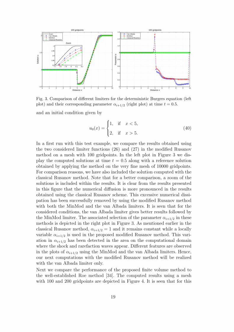
Fig. 3. Comparison of different limiters for the deterministic Burgers equation (leftplot) and their corresponding parameter αi+1/2 (right plot) at time t = 0.5.

and an initial condition given by

u0(x) =

1, if x < 5,

2, if x > 5.(40)

In a first run with this test example, we compare the results obtained usingthe two considered limiter functions (26) and (27) in the modified Rusanovmethod on a mesh with 100 gridpoints. In the left plot in Figure 3 we dis-play the computed solutions at time t = 0.5 along with a reference solutionobtained by applying the method on the very fine mesh of 10000 gridpoints.For comparison reasons, we have also included the solution computed with theclassical Rusanov method. Note that for a better comparison, a zoom of thesolutions is included within the results. It is clear from the results presentedin this figure that the numerical diffusion is more pronounced in the resultsobtained using the classical Rusanov scheme. This excessive numerical dissi-pation has been successfully removed by using the modified Rusanov methodwith both the MinMod and the van Albada limiters. It is seen that for theconsidered conditions, the van Albada limiter gives better results followed bythe MinMod limiter. The associated selection of the parameter αi+1/2 in thesemethods is depicted in the right plot in Figure 3. As mentioned earlier in theclassical Rusanov method, αi+1/2 = 1 and it remains constant while a locallyvariable αi+1/2 is used in the proposed modified Rusanov method. This vari-ation in αi+1/2 has been detected in the area on the computational domainwhere the shock and rarefaction waves appear. Different features are observedin the plots of αi+1/2 using the MinMod and the van Albada limiters. Hence,our next computations with the modified Rusanov method will be realizedwith the van Albada limiter only.

Next we compare the performance of the proposed finite volume method tothe well-established Roe method [34]. The computed results using a meshwith 100 and 200 gridpoints are depicted in Figure 4. It is seen that for this

19

0 1 2 3 4 5 6 7 8 9 100.5

1

1.5

2

Distance x

Sol

utio

n u

100 gridpoints

ExactModified RusanovRoeClassical Rusanov

7.7 7.8 7.9 8 8.1 8.21.8

1.85

1.9

1.95

2

Zoom

0 1 2 3 4 5 6 7 8 9 100.5

1

1.5

2

Distance x

Sol

utio

n u

200 gridpoints

ExactModified RusanovRoeClassical Rusanov

7.7 7.8 7.9 8 8.1 8.21.8

1.85

1.9

1.95

2

Zoom

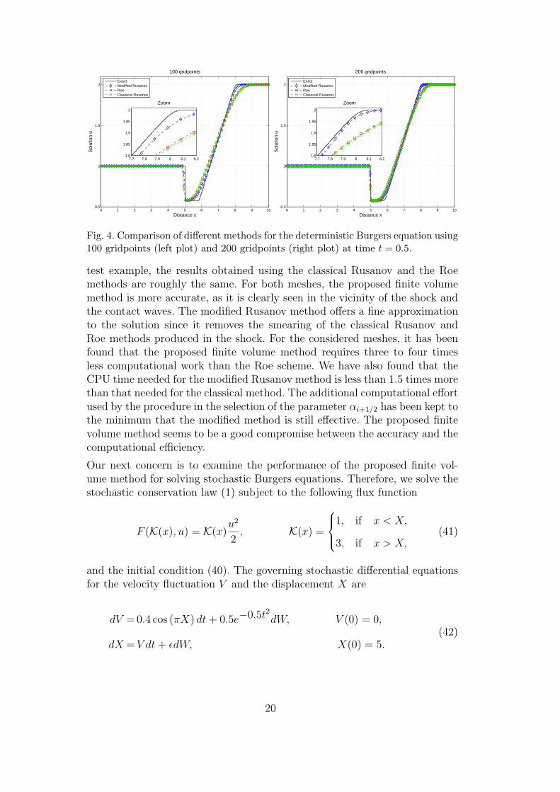
Fig. 4. Comparison of different methods for the deterministic Burgers equation using100 gridpoints (left plot) and 200 gridpoints (right plot) at time t = 0.5.

test example, the results obtained using the classical Rusanov and the Roemethods are roughly the same. For both meshes, the proposed finite volumemethod is more accurate, as it is clearly seen in the vicinity of the shock andthe contact waves. The modified Rusanov method offers a fine approximationto the solution since it removes the smearing of the classical Rusanov andRoe methods produced in the shock. For the considered meshes, it has beenfound that the proposed finite volume method requires three to four timesless computational work than the Roe scheme. We have also found that theCPU time needed for the modified Rusanov method is less than 1.5 times morethan that needed for the classical method. The additional computational effortused by the procedure in the selection of the parameter αi+1/2 has been kept tothe minimum that the modified method is still effective. The proposed finitevolume method seems to be a good compromise between the accuracy and thecomputational efficiency.

Our next concern is to examine the performance of the proposed finite vol-ume method for solving stochastic Burgers equations. Therefore, we solve thestochastic conservation law (1) subject to the following flux function

F (K(x), u) = K(x)u2

2, K(x) =

1, if x < X,

3, if x > X,(41)

and the initial condition (40). The governing stochastic differential equationsfor the velocity fluctuation V and the displacement X are

dV =0.4 cos (πX) dt+ 0.5e−0.5t2dW, V (0) = 0,(42)

dX =V dt+ εdW, X(0) = 5.

20

0 0.1 0.2 0.3 0.4 0.5 0.6 0.7 0.8 0.9 1

4.3

4.4

4.5

4.6

4.7

4.8

4.9

5

5.1

5.2

5.3

Time t

Sol

utio

n X

ε = 0.01

MeanRealization

0 0.1 0.2 0.3 0.4 0.5 0.6 0.7 0.8 0.9 1

4.5

4.6

4.7

4.8

4.9

5

5.1

Time t

Sol

utio

n X

ε = 0.1

MeanRealization

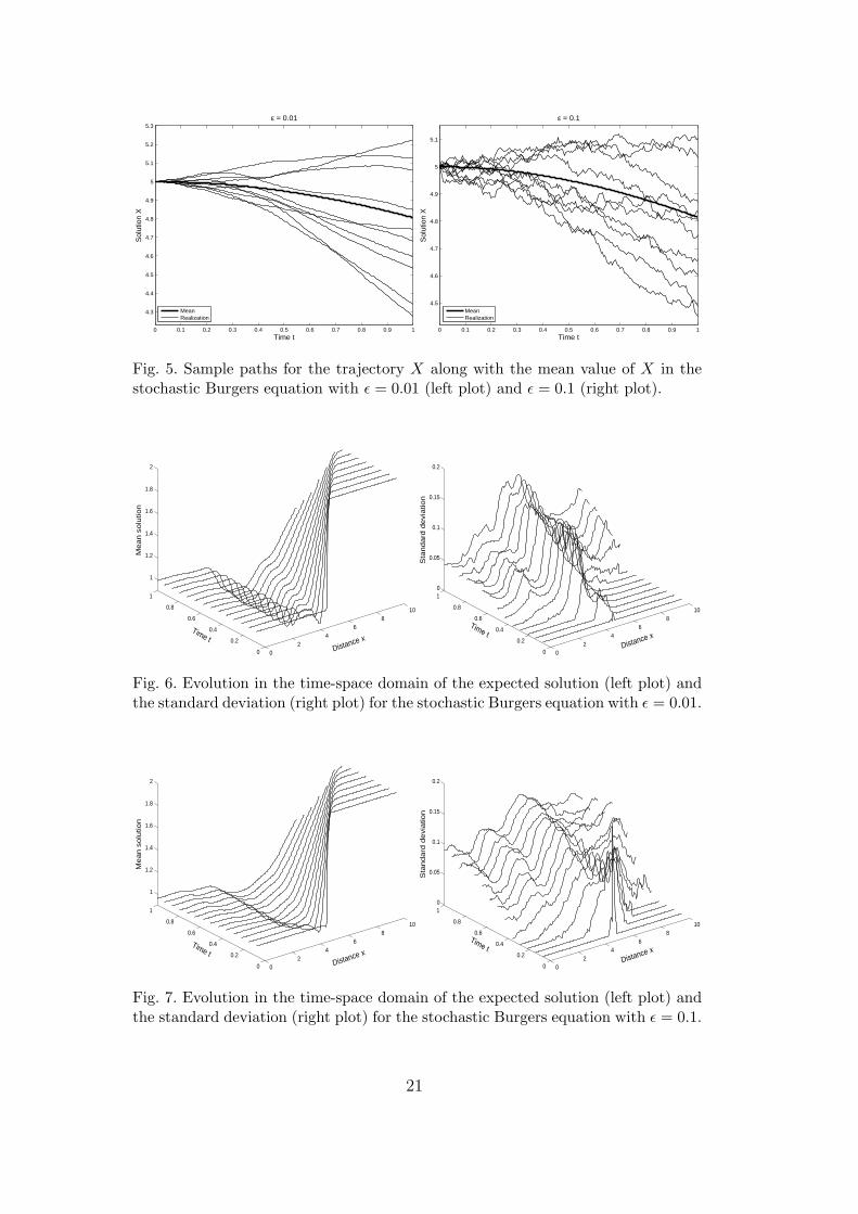
Fig. 5. Sample paths for the trajectory X along with the mean value of X in thestochastic Burgers equation with ε = 0.01 (left plot) and ε = 0.1 (right plot).

02

46

810

0

0.2

0.4

0.6

0.8

1

1

1.2

1.4

1.6

1.8

2

Distance xTime t

Me

an

so

lutio

n

02

46

810

0

0.2

0.4

0.6

0.8

10

0.05

0.1

0.15

0.2

Distance xTime t

Sta

nd

ard

de

via

tion

Fig. 6. Evolution in the time-space domain of the expected solution (left plot) andthe standard deviation (right plot) for the stochastic Burgers equation with ε = 0.01.

02

46

810

0

0.2

0.4

0.6

0.8

1

1

1.2

1.4

1.6

1.8

2

Distance xTime t

Me

an

so

lutio

n

02

46

810

0

0.2

0.4

0.6

0.8

10

0.05

0.1

0.15

0.2

Distance xTime t

Sta

nd

ard

de

via

tion

Fig. 7. Evolution in the time-space domain of the expected solution (left plot) andthe standard deviation (right plot) for the stochastic Burgers equation with ε = 0.1.

21

02

46

810

0

0.2

0.4

0.6

0.8

1

0.8

1

1.2

1.4

1.6

1.8

2

Distance xTime t

Me

an

so

lutio

n

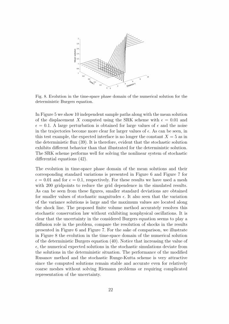
Fig. 8. Evolution in the time-space phase domain of the numerical solution for thedeterministic Burgers equation.

In Figure 5 we show 10 independent sample paths along with the mean solutionof the displacement X computed using the SRK scheme with ε = 0.01 andε = 0.1. A large perturbation is obtained for large values of ε and the noisein the trajectories become more clear for larger values of ε. As can be seen, inthis test example, the expected interface is no longer the constant X = 5 as inthe deterministic flux (39). It is therefore, evident that the stochastic solutionexhibits different behavior than that illustrated for the deterministic solution.The SRK scheme performs well for solving the nonlinear system of stochasticdifferential equations (42).

The evolution in time-space phase domain of the mean solutions and theircorresponding standard variations is presented in Figure 6 and Figure 7 forε = 0.01 and for ε = 0.1, respectively. For these results we have used a meshwith 200 gridpoints to reduce the grid dependence in the simulated results.As can be seen from these figures, smaller standard deviations are obtainedfor smaller values of stochastic magnitudes ε. It also seen that the variationof the variance solutions is large and the maximum values are located alongthe shock line. The proposed finite volume method accurately resolves thisstochastic conservation law without exhibiting nonphysical oscillations. It isclear that the uncertainty in the considered Burgers equation seems to play adiffusion role in the problem, compare the resolution of shocks in the resultspresented in Figure 6 and Figure 7. For the sake of comparison, we illustratein Figure 8 the evolution in the time-space domain of the numerical solutionof the deterministic Burgers equation (40). Notice that increasing the value ofε, the numerical expected solutions in the stochastic simulations deviate fromthe solutions in the deterministic situation. The performance of the modifiedRusanov method and the stochastic Runge-Kutta scheme is very attractivesince the computed solutions remain stable and accurate even for relativelycoarse meshes without solving Riemann problems or requiring complicatedrepresentation of the uncertainty.

22

0 0.5 1 1.5 2 2.5 30.294

0.296

0.298

0.3

0.302

0.304

0.306

Time tvmax

/L

Sol

utio

n X

/L

ε = 0.001

MeanRealization

0 0.5 1 1.5 2 2.5 3

0.22

0.24

0.26

0.28

0.3

0.32

0.34

Time tvmax

/L

Sol

utio

n X

/L

ε = 0.01

MeanRealization

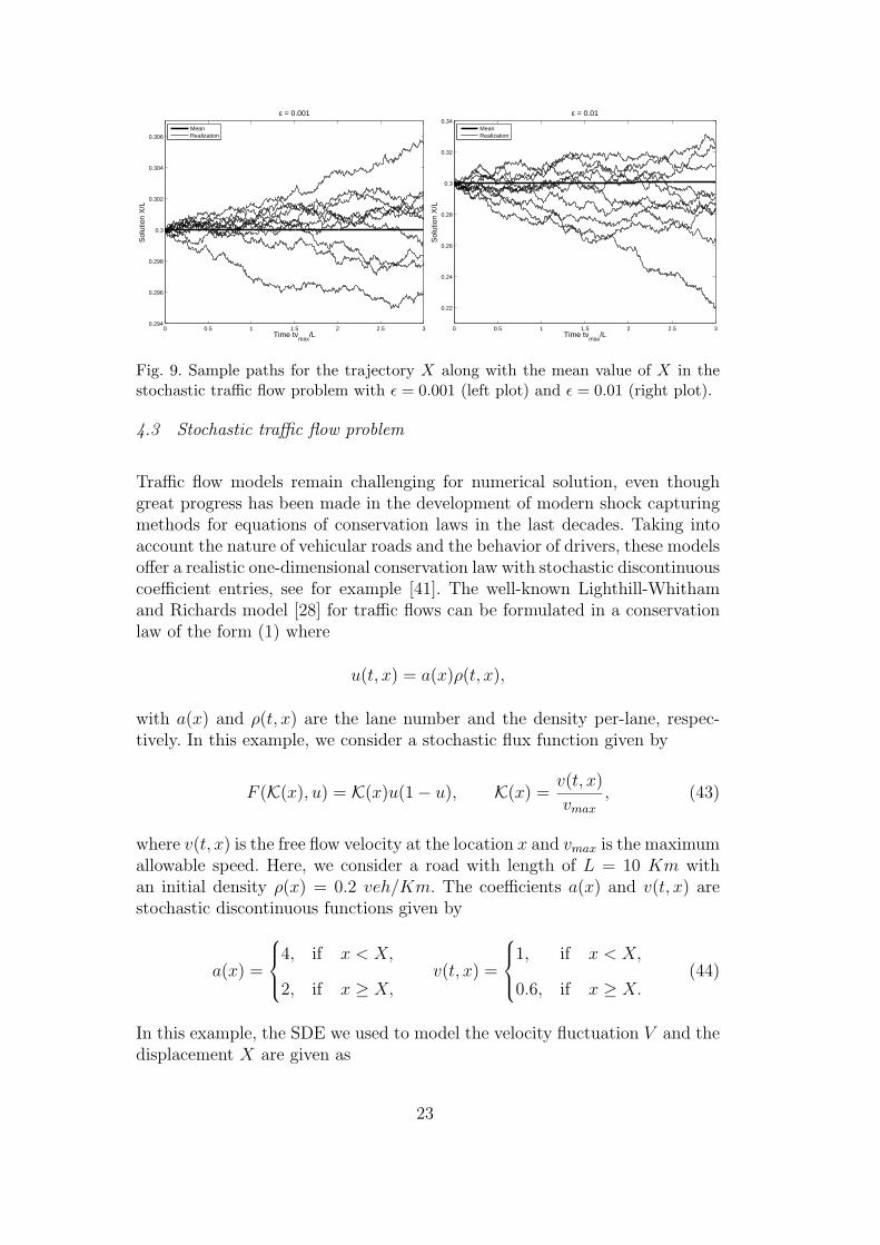
Fig. 9. Sample paths for the trajectory X along with the mean value of X in thestochastic traffic flow problem with ε = 0.001 (left plot) and ε = 0.01 (right plot).

4.3 Stochastic traffic flow problem

Traffic flow models remain challenging for numerical solution, even thoughgreat progress has been made in the development of modern shock capturingmethods for equations of conservation laws in the last decades. Taking intoaccount the nature of vehicular roads and the behavior of drivers, these modelsoffer a realistic one-dimensional conservation law with stochastic discontinuouscoefficient entries, see for example [41]. The well-known Lighthill-Whithamand Richards model [28] for traffic flows can be formulated in a conservationlaw of the form (1) where

u(t, x) = a(x)ρ(t, x),

with a(x) and ρ(t, x) are the lane number and the density per-lane, respec-tively. In this example, we consider a stochastic flux function given by

F (K(x), u) = K(x)u(1− u), K(x) =v(t, x)

vmax, (43)

where v(t, x) is the free flow velocity at the location x and vmax is the maximumallowable speed. Here, we consider a road with length of L = 10 Km withan initial density ρ(x) = 0.2 veh/Km. The coefficients a(x) and v(t, x) arestochastic discontinuous functions given by

a(x) =

4, if x < X,

2, if x ≥ X,v(t, x) =

1, if x < X,

0.6, if x ≥ X.(44)

In this example, the SDE we used to model the velocity fluctuation V and thedisplacement X are given as

23

0 0.1 0.2 0.3 0.4 0.5 0.6 0.7 0.8 0.9 10

0.5

1

1.5

2

2.5

3

0.2

0.3

0.4

0.5

0.6

0.7

0.8

0.9

1

Tim

e tv m

ax/L

Distance x/L

De

nsi

ty ρ

0 0.1 0.2 0.3 0.4 0.5 0.6 0.7 0.8 0.9 10

0.5

1

1.5

2

2.5

3

0

0.05

0.1

0.15

0.2

0.25

0.3

0.35

Tim

e tv m

ax/L

Distance x/L

Sta

ndra

d d

evi

atio

n

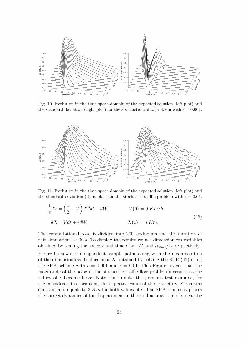
Fig. 10. Evolution in the time-space domain of the expected solution (left plot) andthe standard deviation (right plot) for the stochastic traffic problem with ε = 0.001.

0 0.1 0.2 0.3 0.4 0.5 0.6 0.7 0.8 0.9 10

0.5

1

1.5

2

2.5

3

0.2

0.3

0.4

0.5

0.6

0.7

Tim

e tv

max/L

Distance x/L

De

nsi

ty ρ

0 0.1 0.2 0.3 0.4 0.5 0.6 0.7 0.8 0.9 10

0.5

1

1.5

2

2.5

3

0

0.05

0.1

0.15

0.2

0.25

0.3

0.35

Tim

e tv

max/L

Distance x/L

Sta

nd

rad

de

via

tion

Fig. 11. Evolution in the time-space domain of the expected solution (left plot) andthe standard deviation (right plot) for the stochastic traffic problem with ε = 0.01.

1

εdV =

(1

2− V

)X3dt+ dW, V (0) = 0 Km/h,

(45)dX =V dt+ εdW, X(0) = 3 Km.

The computational road is divided into 200 gridpoints and the duration ofthis simulation is 900 s. To display the results we use dimensionless variablesobtained by scaling the space x and time t by x/L and tvmax/L, respectively.

Figure 9 shows 10 independent sample paths along with the mean solutionof the dimensionless displacement X obtained by solving the SDE (45) usingthe SRK scheme with ε = 0.001 and ε = 0.01. This Figure reveals that themagnitude of the noise in the stochastic traffic flow problem increases as thevalues of ε become large. Note that, unlike the previous test example, forthe considered test problem, the expected value of the trajectory X remainsconstant and equals to 3 Km for both values of ε. The SRK scheme capturesthe correct dynamics of the displacement in the nonlinear system of stochastic

24

0 0.1 0.2 0.3 0.4 0.5 0.6 0.7 0.8 0.9 10

0.5

1

1.5

2

2.5

3

0.2

0.3

0.4

0.5

0.6

0.7

0.8

0.9

1

Tim

e tv m

ax/L

Distance x/L

De

nsi

ty ρ

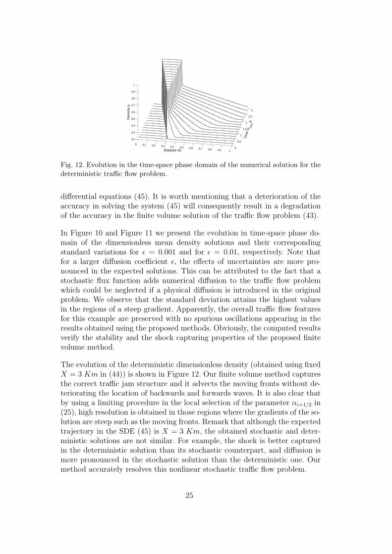
Fig. 12. Evolution in the time-space phase domain of the numerical solution for thedeterministic traffic flow problem.

differential equations (45). It is worth mentioning that a deterioration of theaccuracy in solving the system (45) will consequently result in a degradationof the accuracy in the finite volume solution of the traffic flow problem (43).

In Figure 10 and Figure 11 we present the evolution in time-space phase do-main of the dimensionless mean density solutions and their correspondingstandard variations for ε = 0.001 and for ε = 0.01, respectively. Note thatfor a larger diffusion coefficient ε, the effects of uncertainties are more pro-nounced in the expected solutions. This can be attributed to the fact that astochastic flux function adds numerical diffusion to the traffic flow problemwhich could be neglected if a physical diffusion is introduced in the originalproblem. We observe that the standard deviation attains the highest valuesin the regions of a steep gradient. Apparently, the overall traffic flow featuresfor this example are preserved with no spurious oscillations appearing in theresults obtained using the proposed methods. Obviously, the computed resultsverify the stability and the shock capturing properties of the proposed finitevolume method.

The evolution of the deterministic dimensionless density (obtained using fixedX = 3 Km in (44)) is shown in Figure 12. Our finite volume method capturesthe correct traffic jam structure and it advects the moving fronts without de-teriorating the location of backwards and forwards waves. It is also clear thatby using a limiting procedure in the local selection of the parameter αi+1/2 in(25), high resolution is obtained in those regions where the gradients of the so-lution are steep such as the moving fronts. Remark that although the expectedtrajectory in the SDE (45) is X = 3 Km, the obtained stochastic and deter-ministic solutions are not similar. For example, the shock is better capturedin the deterministic solution than its stochastic counterpart, and diffusion ismore pronounced in the stochastic solution than the deterministic one. Ourmethod accurately resolves this nonlinear stochastic traffic flow problem.

25

0 0.1 0.2 0.3 0.4 0.5 0.6 0.7 0.8

0.5

0.6

0.7

0.8

0.9

1

1.1

1.2

Time t

Sol

utio

n X

ε = 0.01

MeanRealization

0 0.1 0.2 0.3 0.4 0.5 0.6 0.7 0.8

0.4

0.6

0.8

1

1.2

1.4

1.6

Time t

Sol

utio

n X

ε = 0.4

MeanRealization

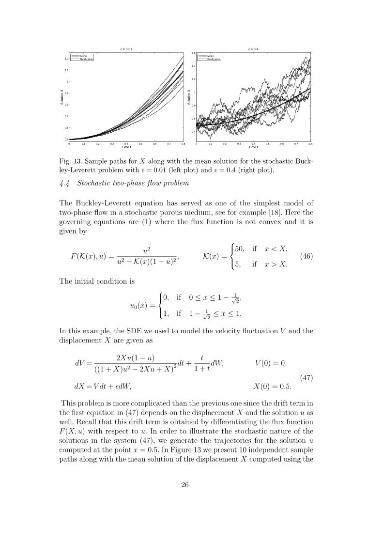
Fig. 13. Sample paths for X along with the mean solution for the stochastic Buck-ley-Leverett problem with ε = 0.01 (left plot) and ε = 0.4 (right plot).

4.4 Stochastic two-phase flow problem

The Buckley-Leverett equation has served as one of the simplest model oftwo-phase flow in a stochastic porous medium, see for example [18]. Here thegoverning equations are (1) where the flux function is not convex and it isgiven by

F (K(x), u) =u2

u2 +K(x)(1− u)2, K(x) =

50, if x < X,

5, if x > X.(46)

The initial condition is

u0(x) =

0, if 0 ≤ x ≤ 1− 1√

2,

1, if 1− 1√2≤ x ≤ 1.

In this example, the SDE we used to model the velocity fluctuation V and thedisplacement X are given as

dV =2Xu(1− u)

((1 +X)u2 − 2Xu+X)2dt+

t

1 + tdW, V (0) = 0,

(47)dX =V dt+ εdW, X(0) = 0.5.

This problem is more complicated than the previous one since the drift term inthe first equation in (47) depends on the displacement X and the solution u aswell. Recall that this drift term is obtained by differentiating the flux functionF (X, u) with respect to u. In order to illustrate the stochastic nature of thesolutions in the system (47), we generate the trajectories for the solution ucomputed at the point x = 0.5. In Figure 13 we present 10 independent samplepaths along with the mean solution of the displacement X computed using the

26

0

0.2

0.4

0.6

0.8

1

0

0.2

0.4

0.6

0.80

0.2

0.4

0.6

0.8

1

Distance xTime t

Me

an

so

lutio

n

0

0.2

0.4

0.6

0.8

1

0

0.2

0.4

0.6

0.80

0.02

0.04

0.06

0.08

0.1

0.12

0.14

Distance x

Time t

Sta

nd

ard

de

via

tion

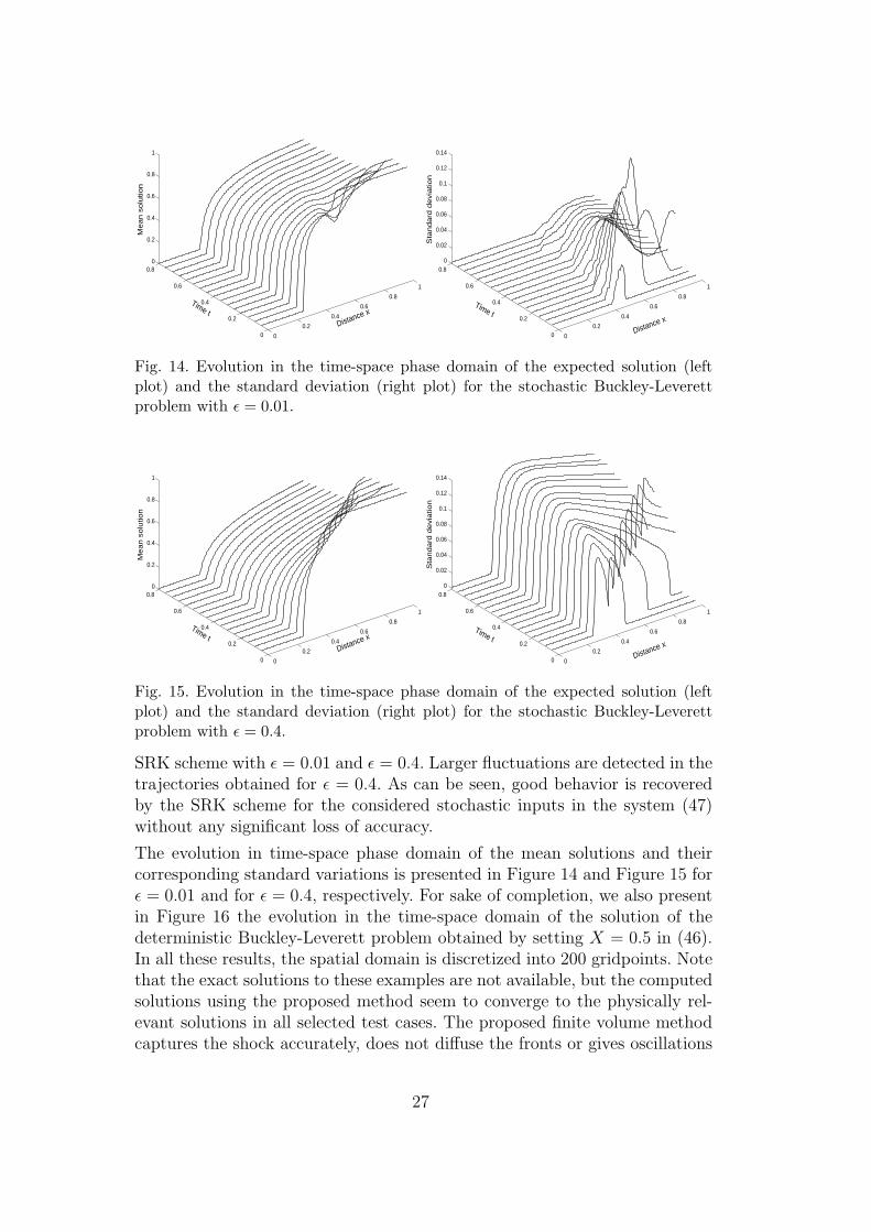
Fig. 14. Evolution in the time-space phase domain of the expected solution (leftplot) and the standard deviation (right plot) for the stochastic Buckley-Leverettproblem with ε = 0.01.

0

0.2

0.4

0.6

0.8

1

0

0.2

0.4

0.6

0.80

0.2

0.4

0.6

0.8

1

Distance xTime t

Me

an

so

lutio

n

0

0.2

0.4

0.6

0.8

1

0

0.2

0.4

0.6

0.80

0.02

0.04

0.06

0.08

0.1

0.12

0.14

Distance x

Time t

Sta

nd

ard

de

via

tion

Fig. 15. Evolution in the time-space phase domain of the expected solution (leftplot) and the standard deviation (right plot) for the stochastic Buckley-Leverettproblem with ε = 0.4.

SRK scheme with ε = 0.01 and ε = 0.4. Larger fluctuations are detected in thetrajectories obtained for ε = 0.4. As can be seen, good behavior is recoveredby the SRK scheme for the considered stochastic inputs in the system (47)without any significant loss of accuracy.

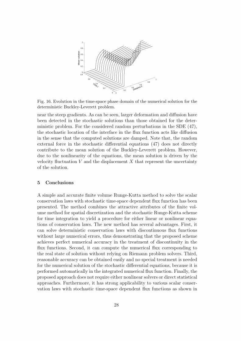
The evolution in time-space phase domain of the mean solutions and theircorresponding standard variations is presented in Figure 14 and Figure 15 forε = 0.01 and for ε = 0.4, respectively. For sake of completion, we also presentin Figure 16 the evolution in the time-space domain of the solution of thedeterministic Buckley-Leverett problem obtained by setting X = 0.5 in (46).In all these results, the spatial domain is discretized into 200 gridpoints. Notethat the exact solutions to these examples are not available, but the computedsolutions using the proposed method seem to converge to the physically rel-evant solutions in all selected test cases. The proposed finite volume methodcaptures the shock accurately, does not diffuse the fronts or gives oscillations

27

0

0.2

0.4

0.6

0.8

1

0

0.2

0.4

0.6

0.80

0.2

0.4

0.6

0.8

1

Distance xTime t

Me

an

so

lutio

n

Fig. 16. Evolution in the time-space phase domain of the numerical solution for thedeterministic Buckley-Leverett problem.

near the steep gradients. As can be seen, larger deformation and diffusion havebeen detected in the stochastic solutions than those obtained for the deter-ministic problem. For the considered random perturbations in the SDE (47),the stochastic location of the interface in the flux function acts like diffusionin the sense that the computed solutions are damped. Note that, the randomexternal force in the stochastic differential equations (47) does not directlycontribute to the mean solution of the Buckley-Leverett problem. However,due to the nonlinearity of the equations, the mean solution is driven by thevelocity fluctuation V and the displacement X that represent the uncertaintyof the solution.

5 Conclusions

A simple and accurate finite volume Runge-Kutta method to solve the scalarconservation laws with stochastic time-space dependent flux function has beenpresented. The method combines the attractive attributes of the finite vol-ume method for spatial discretization and the stochastic Runge-Kutta schemefor time integration to yield a procedure for either linear or nonlinear equa-tions of conservation laws. The new method has several advantages. First, itcan solve deterministic conservation laws with discontinuous flux functionswithout large numerical errors, thus demonstrating that the proposed schemeachieves perfect numerical accuracy in the treatment of discontinuity in theflux functions. Second, it can compute the numerical flux corresponding tothe real state of solution without relying on Riemann problem solvers. Third,reasonable accuracy can be obtained easily and no special treatment is neededfor the numerical solution of the stochastic differential equations, because it isperformed automatically in the integrated numerical flux function. Finally, theproposed approach does not require either nonlinear solvers or direct statisticalapproaches. Furthermore, it has strong applicability to various scalar conser-vation laws with stochastic time-space dependent flux functions as shown in

28

the numerical results.

The proposed finite volume Runge-Kutta method has been tested on stochas-tic Burgers equation, stochastic problems in traffic flow and two-phase flowapplications. The obtained results indicate good shock resolution with highaccuracy in smooth regions and without any nonphysical oscillations near theshock areas. The convergence to the correct steady-state solution has beenclearly verified in a deterministic scalar conservation law with discontinuousflux function. Results presented in this paper have show high resolution ofthe proposed finite volume method and confirm its capability to provide accu-rate and efficient simulations for scalar conservation laws with stochastic time-space dependent flux functions. Future work will concentrate on extending theproposed method to hyperbolic systems of conservation laws with stochastictime-space dependent flux function in one and two space dimensions. Further-more, since the difficulties arising from coefficients with multiplicative noisewould not fit into the frame of this paper, we will only deal with stochasticconservation laws involving multiplicative noise in a forthcoming paper.

Acknowledgment. This work was partly performed while the second authorwas a visiting professor at department of mathematics, university of Taibahat Madinah. M. Seaid is deeply grateful to the Taibah university for theirhospitality during a research visit there.

References

[1] B. Andreianov, K. Karlsen, N. Risebro, A theory of L1-dissipative solvers forscalar conservation laws with discontinuous flux, Archive Rat. Mech. Anal. 201(2011) 27–86.

[2] C. Archubi, L. Braunstein, R. Buceta, Growing interfaces in quenched media:stochastic differential equation, Physica A: Statistical Mechanics and itsApplications 283 (2000) 204–207.

[3] I. Bonzani, L. Mussone, Stochastic modelling of traffic flow, Mathematical andComputer Modelling 36 (2002) 109–119.

[4] A. Debussche, J. Vovelle, Scalar conservation laws with stochastic forcing,Journal of Functional Analysis 259 (2010) 1014–1042.

[5] P. Degond, C. Ringhofer, Stochastic dynamics of long supply chains withrandom breakdowns, SIAM J. Appl. Anal. 68 (2007) 59–79.

[6] S. Diehl, A conservation law with point source and discontinuous flux function,SIAM J. Math. Anal. 56 (1996) 388–419.

[7] J. Feng, D. Nualart, Stochastic scalar conservation laws, J. Funct. Anal. 255(2008) 313–373.

29

[8] S. Frank, W. Schmickler, Ion transfer across liquidliquid interfaces fromtransition-state theory and stochastic molecular dynamics simulations, J.Electroanalytical Chemistry 590 (2006) 138–144.

[9] R. Ghanem, P. Spanos, Stochastic Finite Elements: A Spectral Approach,Springer-Verlag, New York, 1991.

[10] T. Gimse, N. Risebro, Solution of Cauchy problem for a conservation law witha discontinuous flux function, SIAM J. Math. Anal. 23 (1992) 635–648.

[11] D. Gottlieb, D. Xiu, Galerkin method for wave equations with uncertaincoefficients, Comm. Comput. Phys. 3 (2008) 505–518.

[12] S. Heinz, Statistical Mechanics of Turbulent Flows, Springer-Verlag, Berlin,2003.

[13] H. Holden, N. Risebro, On the stochastic Buckley-Leverett equation, SIAM J.Appl. Math. 51 (1991) 1472–1488.

[14] H. Holden, N. Risebro, A stochastic approach to conservation laws, In: ThirdInternational Conference on Hyperbolic Problems. Theory, Numerical Methodsand Applications, Uppsala Eds. B. Engquist, B. Gustafsson (1991) 575–587.

[15] H. Holden, N. Risebro, A mathematical model of traffic flow on a network ofunidirectional roads, SIAM J. Math. Anal. 26 (1995) 999–1017.

[16] H. Holden, N. Risebro, Conservation laws with a random source, Appl. Math.Optim. 36 (1997) 229–241.

[17] H. Holden, B. ∅ksendal, J. Ub∅e, T. Zhang, Stochastic Partial DifferentialEquations: A Modeling, White Noise Functional Approach, Springer-Verlag,1996.

[18] L. Holden, The Buckley-Leverett equation with spatially stochastic fluxfunction, SIAM J. Appl. Anal. 57 (1997) 1443–1454.

[19] T. Hou, W. Luo, B. Rozovski, H. Zhou, Wiener chaos expansions and numericalsolutions of randomly forced equations of fluid mechanics, J. Comput. Physics.216 (2006) 687–706.

[20] J. Hurtado, A. Barbat, Monte Carlo techniques in computational stochatsicmechanics, Arch. Comput. Methods Engrg. 5 (1998) 3–29.

[21] E. Isaacson, B. Temple, Analysis of a singular hyperbolic system of conservationlaws, J. Diff. Equations. 65 (1986) 250–268.

[22] A. Jazwinski, Stochastic Processes and Filtering Theory, Academic Press, NewYork, 1970.

[23] P. Jenny, M. Torrilhon, S. Heinz, A solution algorithm for the fluid dynamicequations based on a stochastic model for molecular motion, J. Comput.Physics. 229 (2010) 1077–1098.

30

[24] M. Kaminski, Stochastic boundary element method analysis of the interfacedefects in composite materials, Composite Structures 94 (2012) 394–402.

[25] K. Karlsen, C. Klingenberg, N. Risebro, A relaxation scheme for conservationlaws with a discontinuous coefficient, Math. Comp. 73 (2003) 1235–1259.

[26] P. Kloeden, E. Platen, The Numerical Solution of Stochastic DifferentialEquations, Springer Verlag, Berlin, 1999.

[27] B. V. Leer, Towards the ultimate conservative difference schemes v. a second-order sequal to Godunov’s method, J. Comp. Phys. 32 (1979) 101–136.

[28] M. Lighthill, J. Whitham, On kinematic waves: II. a theory of traffic flow onlong crowded roads, Proc. Royal. Soc. London, Series A. 229 (1955) 317–345.

[29] H. Manouzi, M. Seaıd, M. Zahri, Wick-stochastic finite element solution ofreaction-diffusion problems, J. Comp. Applied Math. 203 (2007) 516–532.

[30] K. Mohamed, Simulation numerique en volume finis, de problemesd’ecoulements multidimensionnels raides, par un schema de flux a deux pas,Dissertation, University of Paris 13, 2005.

[31] S. Osher, R. Fedkiw, Level Set Methods and Dynamic Implicit Surfaces,Springer-Verlag, Berlin, 2003.

[32] G. Poette, B. Despres, D. Lucor, Uncertainty quantification for systems ofconservation laws, J. Comp. Phys. 228 (2009) 2443–2467.

[33] J. L. Randall, Numerical Methods for Conservation Laws, Lectures inMathematics ETH Zurich, 1992.

[34] P. Roe, Approximate riemann solvers, parameter vectors and difference schemes,J. Comp. Physics. 43 (1981) 357–372.

[35] A. Roßler, Rooted tree analysis for order conditions of stochastic Runge-Kutta methods for the weak approximation of stochastic differential equations,Stochastic Anal. Appl. 24 (2006) 97–134.

[36] A. Roßler, Runge-Kutta methods for I to stochastic differential equations withscalar noise, BIT 46 (2006) 97–110.

[37] A. Roßler, Second order Runge-Kutta methods for Ito stochastic differentialequations, SIAM J. Numer. Anal. 47 (2009) 1713–1738.

[38] V. Rusanov, Calculation of interaction of non-steady shock waves withobstacles, J. Comp. Math. Phys. USSR 1 (1961) 267–279.

[39] M. Seaıd, Stable numerical methods for conservation laws with discontinuousflux function, Appl. Math. Comput. 175 (2006) 383–400.

[40] M. Serrano, K. Klemm, F. Vazquez, V. Eguıluz, M. S. Miguel, Conservationlaws for voter-like models on random directed networks, J. Stat. Mech. 2009(2009) P10024.

31

[41] A. Sopasakis, Stochastic noise approach to traffic flow modeling, Physica A 342(2004) 741–754.

[42] P. Sweby, High resolution schemes using flux limiters for hyperbolic conservationlaws, SIAM J. Numer. Anal. 21 (1984) 995–1011.

[43] T. Tang, T. Zhou, Convergence analysis for stochastic collocation methods toscalar hyperbolic equations with a random wave speed, Commun. Comput.Phys. 8 (2010) 226–248.

[44] J. Tryoen, O. L. Maitre, A. Ern, Adaptive anisotropic spectral stochasticmethods for uncertain scalar conservation laws, SIAM J. Sci. Comp. To appear.

[45] J. Tryoen, O. L. Maitre, M. Ndjinga, A. Ern, Roe solver with entropy correctorfor uncertain hyperbolic systems, J. Comput. App. Math. 235 (2010) 491–506.

[46] K. Waldeer, A numeric investigation of a vehicular traffic flow model based on astochastic acceleration process, Computer Physics Communications 147 (2002)650–653.

[47] D. Yang, J. Zhang, Z. Lu, Stochastic analysis of saturated-unsaturatedflow in heterogeneous media by combining Karhunen-Loeve expansion andperturbation method, J. Hydrology. 294 (2004) 18–38.

[48] T. Zhou, Stochastic Galerkin methods for elliptic interface problems withrandom input, J. Comput. App. Math. 236 (2011) 782–792.

[49] T. Zhou, T. Tang, Galerkin methods for stochastic hyperbolic problems usingbi-orthogonal polynomials, J. Sci. Comput. 51 (2012) 274–292.

32