A Finite Variable Difference Relaxation Scheme for hyperbolic–parabolic equations Mayank Bajpayi, S.V. Raghurama Rao * CFD Centre, Department of Aerospace Engineering, Indian Institute of Science, Bangalore, Karnataka 560012, India article info Article history: Received 5 December 2007 Received in revised form 20 March 2009 Accepted 23 June 2009 Available online 5 July 2009 Keywords: Finite Variable Difference Method Relaxation systems Relaxation schemes Nonlinear hyperbolic–parabolic equations Vector conservation laws Shallow water equations abstract Using the framework of a new relaxation system, which converts a nonlinear viscous con- servation law into a system of linear convection–diffusion equations with nonlinear source terms, a finite variable difference method is developed for nonlinear hyperbolic–parabolic equations. The basic idea is to formulate a finite volume method with an optimum spatial difference, using the Locally Exact Numerical Scheme (LENS), leading to a Finite Variable Difference Method as introduced by Sakai [Katsuhiro Sakai, A new finite variable difference method with application to locally exact numerical scheme, Journal of Computational Physics, 124 (1996) pp. 301–308.], for the linear convection–diffusion equations obtained by using a relaxation system. Source terms are treated with the well-balanced scheme of Jin [Shi Jin, A steady-state capturing method for hyperbolic systems with geometrical source terms, Mathematical Modeling Numerical Analysis, 35 (4) (2001) pp. 631–645]. Bench-mark test problems for scalar and vector conservation laws in one and two dimen- sions are solved using this new algorithm and the results demonstrate the efficiency of the scheme in capturing the flow features accurately. Ó 2009 Elsevier Inc. All rights reserved. 1. Introduction Numerical solution of hyperbolic and parabolic partial differential equations has reached a state of maturity in the past few decades. A major contribution to this progress came from the researchers in Computational Fluid Dynamics (CFD). The numerical solution of Euler equations of gas dynamics and the shallow water equations, which represent hyperbolic vector conservation laws, is now considered to be an established field, with several innovative numerical methods having been introduced in the past few decades. Some reviews of this history are available in [16,17,25,47,27]. One major focus in this development has been the introduction of higher order accurate methods which are stable and are free of numerical oscil- lations. The Total Variation Diminishing (TVD) schemes with limiters are especially designed for this purpose. However, dif- ficulties still remain with this approach: getting uniformly higher order accuracy in all parts of the computational domain without clipping of the extrema, especially in multi-dimensions and with unstructured meshes, is hard to achieve and the research is still continuing in this area, as can be seen from the large number of papers continuously being published. The reader is referred to the books edited by Hussaini, van Leer and Rosendale [19], Barth and Deconink [5] and the refer- ences therein for a glimpse of these developments. One of the essential difficulties associated with higher order schemes for convection dominated flow simulations is the nonmonotonicity of the solutions, manifesting as oscillations or wiggles, especially near high gradient regions or disconti- nuities. In this context, an important early development was the Godunov theorem [10] in which it was shown that linear 0021-9991/$ - see front matter Ó 2009 Elsevier Inc. All rights reserved. doi:10.1016/j.jcp.2009.06.038 * Corresponding author. Tel.: +91 80 2293 3031; fax: +91 80 23600134. E-mail addresses: [email protected], [email protected] (S.V. Raghurama Rao). Journal of Computational Physics 228 (2009) 7513–7542 Contents lists available at ScienceDirect Journal of Computational Physics journal homepage: www.elsevier.com/locate/jcp

Welcome message from author
This document is posted to help you gain knowledge. Please leave a comment to let me know what you think about it! Share it to your friends and learn new things together.
Transcript
Journal of Computational Physics 228 (2009) 7513–7542
Contents lists available at ScienceDirect
Journal of Computational Physics
journal homepage: www.elsevier .com/locate / jcp
A Finite Variable Difference Relaxation Schemefor hyperbolic–parabolic equations
Mayank Bajpayi, S.V. Raghurama Rao *
CFD Centre, Department of Aerospace Engineering, Indian Institute of Science, Bangalore, Karnataka 560012, India
a r t i c l e i n f o
Article history:Received 5 December 2007Received in revised form 20 March 2009Accepted 23 June 2009Available online 5 July 2009
Keywords:Finite Variable Difference MethodRelaxation systemsRelaxation schemesNonlinear hyperbolic–parabolic equationsVector conservation lawsShallow water equations
0021-9991/$ - see front matter � 2009 Elsevier Incdoi:10.1016/j.jcp.2009.06.038
* Corresponding author. Tel.: +91 80 2293 3031;E-mail addresses: [email protected], svrag
a b s t r a c t
Using the framework of a new relaxation system, which converts a nonlinear viscous con-servation law into a system of linear convection–diffusion equations with nonlinear sourceterms, a finite variable difference method is developed for nonlinear hyperbolic–parabolicequations. The basic idea is to formulate a finite volume method with an optimum spatialdifference, using the Locally Exact Numerical Scheme (LENS), leading to a Finite VariableDifference Method as introduced by Sakai [Katsuhiro Sakai, A new finite variable differencemethod with application to locally exact numerical scheme, Journal of ComputationalPhysics, 124 (1996) pp. 301–308.], for the linear convection–diffusion equations obtainedby using a relaxation system. Source terms are treated with the well-balanced scheme ofJin [Shi Jin, A steady-state capturing method for hyperbolic systems with geometricalsource terms, Mathematical Modeling Numerical Analysis, 35 (4) (2001) pp. 631–645].Bench-mark test problems for scalar and vector conservation laws in one and two dimen-sions are solved using this new algorithm and the results demonstrate the efficiency of thescheme in capturing the flow features accurately.
� 2009 Elsevier Inc. All rights reserved.
1. Introduction
Numerical solution of hyperbolic and parabolic partial differential equations has reached a state of maturity in the pastfew decades. A major contribution to this progress came from the researchers in Computational Fluid Dynamics (CFD). Thenumerical solution of Euler equations of gas dynamics and the shallow water equations, which represent hyperbolic vectorconservation laws, is now considered to be an established field, with several innovative numerical methods having beenintroduced in the past few decades. Some reviews of this history are available in [16,17,25,47,27]. One major focus in thisdevelopment has been the introduction of higher order accurate methods which are stable and are free of numerical oscil-lations. The Total Variation Diminishing (TVD) schemes with limiters are especially designed for this purpose. However, dif-ficulties still remain with this approach: getting uniformly higher order accuracy in all parts of the computational domainwithout clipping of the extrema, especially in multi-dimensions and with unstructured meshes, is hard to achieve andthe research is still continuing in this area, as can be seen from the large number of papers continuously being published.The reader is referred to the books edited by Hussaini, van Leer and Rosendale [19], Barth and Deconink [5] and the refer-ences therein for a glimpse of these developments.
One of the essential difficulties associated with higher order schemes for convection dominated flow simulations is thenonmonotonicity of the solutions, manifesting as oscillations or wiggles, especially near high gradient regions or disconti-nuities. In this context, an important early development was the Godunov theorem [10] in which it was shown that linear
. All rights reserved.
fax: +91 80 [email protected] (S.V. Raghurama Rao).
7514 M. Bajpayi, S.V. Raghurama Rao / Journal of Computational Physics 228 (2009) 7513–7542
higher order schemes would necessarily lead to nonmonotone solutions. A way to circumvent this limitation is to make thecoefficients nonlinear, by making the coefficients depend on the solution variables. The Flux Corrected Transport (FCT) algo-rithm of Boris and Book [6–8,53] and the Monotone Upstream Schemes for Conservation Laws (MUSCL) methodology of vanLeer [48–51] are based on this strategy (see also [13]). Harten introduced the popular Total Variation Diminishing (TVD)schemes [14] by providing a rigorous mathematical foundation for this approach which was further developed by Sweby[46] and a lot of other researchers (see [19] for details). Goodman and Leveque [11] showed that multi-dimensional TVDschemes are no better than first order accurate schemes. Later, Essentially NonOscillatory (ENO) schemes were developedto overcome some of the deficiencies of the TVD schemes like clipping the extrema [15]. A detailed account of the furtherdevelopment of ENO schemes is given by Shu [44]. In spite of their advantages over TVD methods, ENO methods are notso convenient to extend to multi-dimensions. The development of higher order schemes is far from complete and the re-search in this area is still continuing; according to Roe [39], rigor is not yet to be found in all aspects of higher order schemes.In this context, it is worth looking for alternative approaches.
In the process of discretization of the convection dominated equations in CFD, it is considered advantageous to mimic theproperties of the exact solutions of the original equations (when they are available) so that the resulting discretized equa-tions have better chance to converge to the physically relevant solutions. For example, the upwind methods mimic the exactsolutions of convection equations as closely as possible in a finite difference framework. An interesting alternative to thisstrategy is to develop a numerical method in which the coefficients in the difference equation satisfy the exact solutionof the original convection (or convection–diffusion) equation. Some numerical methods using this strategy were developedby Allen and Southwell [1], Günther [12] and Sakai [40]. A related idea is used in Nonstandard Finite Difference Methods ofMickens [31] in which the difference equations have the same general solutions as the associated differential equations.An attempt to apply this approach to nonlinear convection equations and linear systems of convection equations is givenin [52]. These methods produce results which are very close to the exact solutions, many times producing much superiorresults compared to traditional finite difference methods.
The Finite Variable Difference Method (FVDM) of Sakai [41] is one such interesting alternative to the traditional ap-proaches. In this method, a nonoscillatory algorithm is developed for convection–diffusion equations, based on a variablemesh increment, with the optimal spatial difference being determined by minimizing the variance of the solution by choos-ing the roots of the difference equation to be nonnegative. Sakai [41,43] has demonstrated the efficiency of the FVDM forlinear convection–diffusion problems and derived some new schemes based on this strategy for the 1-D Burgers equation,in which the hyperbolic terms are nonlinear. An important feature of the FVDM is that a nonoscillatory scheme is formulatedexplicitly based on the exact solution of convection–diffusion equations, a feature not shared by the convectional higher or-der schemes such as TVD methods. Note that in this scheme, the formulation of a nonoscillatory scheme is done directly forconvection–diffusion equations, whereas most of the TVD methods are formulated only for convection equations. Anotherimportant feature of the FVDM is that the drive towards accuracy in developing a nonoscillatory scheme is based on min-imizing the variance of the solution, variance being the deviation from the exact solution, which is more reasonable touse compared to the conventional derivation based on Taylor series expansions in the finite difference methods [41]. Yetanother interesting feature of the FVDM is that formulation of the scheme is not based explicitly on artificial viscosity. Sakai[41] has demonstrated that the oscillations in the solutions are completely avoided by the FVDM in the case of steady equa-tions and only very mild oscillations appear in the unsteady case. Because of all the above features, the FVDM is selected inthis work, as an interesting alternative for study in developing accurate numerical methods for hyperbolic–parabolic partialdifferential equations representing conservation/balance laws.
Extending the FVDM directly to the unsteady and nonlinear Burgers equation seems to be nontrivial. So far, the FVDM hasalso not been applied to the hyperbolic systems of conservation laws. In this study, we extend Sakai’s Finite Variable Differ-ence Method to nonlinear Burgers equation, and also to a hyperbolic system of conservation laws (shallow water equations),by coupling this method to a new relaxation system which modifies the relaxation system of Jin and Xin [20], while linear-izing the nonlinear hyperbolic–parabolic equations. We utilize the strategy used by Sakai, by applying FVDM to the LocallyExact Numerical Scheme in which the difference coefficients are determined such that the resulting difference equation sat-isfies the exact solution of the convection–diffusion equation, in our frame work of a novel relaxation system applied to thenonlinear convection–diffusion equations. This Finite Variable Difference Relaxation Scheme (FVDRS) is tested on some bench-mark test problems for 1-d inviscid Burgers equation, 1-D viscous Burgers equation, 2-D inviscid Burgers equation, 2-D vis-cous Burgers equation and shallow water equations in both one and two dimensions. The results demonstrate the efficiencyof this Finite Variable Difference Relaxation Method. It is worth noting that our method is not based on Riemann solvers, whichare reported to be associated with a list of failures [34].
2. A relaxation system for viscous Burgers equation
Jin and Xin [20] introduced a relaxation system for hyperbolic equations like inviscid Burgers equation or Euler equations.A relaxation system provides a vanishing viscosity model for nonlinear hyperbolic conservation laws by replacing the non-linear hyperbolic (convection) terms with linear hyperbolic terms with a stiff nonlinear source term which represents amathematical relaxation process. The relaxation schemes, based on a relaxation system, are interesting alternatives to tra-ditional schemes for solving hyperbolic conservation laws. The reader is referred to [20,32,2,26,36,37,4] for some numerical
M. Bajpayi, S.V. Raghurama Rao / Journal of Computational Physics 228 (2009) 7513–7542 7515
methods based on relaxation systems. Extending the relaxation systems to hyperbolic–parabolic systems representing con-vection–diffusion systems or viscous conservation laws is a nontrivial task. Lions and Toscani [28], Jin, Pareschi and Toscani[21], Jin [22], Raghurama Rao [35] (see also [38]) and Aregba-Driollet, Natalini and Tang [3] introduced some relaxation sys-tems for hyperbolic–parabolic equations and corresponding numerical methods for viscous conservation laws. In this sec-tion, we introduce a new relaxation system for the viscous Burgers equation, by treating the viscous term as a source term.
Consider the viscous Burgers equation, given by
ouotþ ogðuÞ
ox¼ ogvðuÞ
oxð1Þ
Here the flux gðuÞ is a nonlinear function of the dependent variable u (since gðuÞ ¼ 12 u2) and gvðuÞ is viscous flux (gvðuÞ ¼ m ou
ox).The above nonlinear partial differential equation is converted into two linear partial differential equations with a nonlinearrelaxation term by introducing a new variable v (for the nonlinear flux gðuÞ) as
ouotþ ov
ox¼ ogvðuÞ
oxð2Þ
ovotþ k2 ou
ox¼ � ½v � gðuÞ�
�ð3Þ
where k is a positive constant (relaxation parameter) and � is a small parameter such that �! 0. When �! 0, the secondequation of the relaxation system (3) gives v ¼ gðuÞ, which when substituted into the first Eq. (2), gives back the viscousBurgers equation (1). Thus, solving (2) and (3) in the limit of �! 0 is equivalent to solving (1). The advantage lies in the factthat the relaxation system (2) and (3) is linear in convection terms (on the left hand side) and is easy to deal with. The righthand side of the relaxation system is still nonlinear due to the relaxation term, but if we use the splitting method, the aboverelaxation system can be split into a linear system of convection equations and an ordinary differential equation (containingthe nonlinear term), both of which can be easily solved.
The above relaxation system can be written in vector form as
oQotþ A
oQox¼ H ð4Þ
where
Q ¼u
v
� �; A ¼
0 1k2 0
� �and H ¼
@gvðuÞ@x
�½v�gðuÞ��
" #ð5Þ
Since Eq. (4) has linear hyperbolic terms on the left hand side, we can use the characteristic variables to obtain a set of decou-pled equations. We can write
A ¼ RKR�1 and thus K ¼ R�1AR ð6Þ
where R is the matrix of right eigenvectors of A, R�1 is its inverse and K is a diagonal matrix with eigenvalues of A as its ele-ments. The expressions for R, R�1 and K are given by
R ¼1 1�k k
� �; R�1 ¼
12
�12k
12
12k
" #and K ¼
�k 00 k
� �ð7Þ
Introducing f as a characteristic variable vector given by
f ¼ R�1Q ð8Þ
we obtain from the vector form of the relaxation system (4) the decoupled system as
ofotþK
ofox¼ R�1H ð9Þ
where
f ¼f1
f2
� �¼
u2� v
2ku2þ v
2k
" #and R�1H ¼
12
ogvðuÞox þ
v�gðuÞ2�
12
ogvðuÞox �
v�gðuÞ2�
" #ð10Þ
Thus we obtain two decoupled equations as
of1
ot� k
of1
ox¼ 1
2ogvðuÞ
oxþ ½v � gðuÞ�
2k�of2
otþ k
of2
ox¼ 1
2ogvðuÞ
ox� ½v � gðuÞ�
2k�ð11Þ
7516 M. Bajpayi, S.V. Raghurama Rao / Journal of Computational Physics 228 (2009) 7513–7542
The original variable u and v can be recovered as
u ¼ f1 þ f2 and v ¼ kðf2 � f1Þ ð12Þ
and thus we obtainogvðuÞox
¼ mo2uox2 ¼ m
o2f1
ox2 þ mo2f2
ox2 ð13Þ
Thus, the decoupled equations become
of1
ot� k
of1
ox¼ 1
2m
o2f1
ox2 þ12m
o2f2
ox2 þ½v � gðuÞ�
2k�ð14Þ
of2
otþ k
of2
ox¼ 1
2m
o2f2
ox2 þ12m
o2f1
ox2 �½v � gðuÞ�
2k�ð15Þ
Eqs. (14) and (15) are convection diffusion equations with source terms. Note that the convection parts of the equations arenow linear, unlike the original viscous Burgers equation in which the convection terms are nonlinear. Let us now rewritethese equations by introducing new variables F1 and F2 as
F ¼F1
F2
� �¼
12 u� 1
2k gðuÞ12 uþ 1
2k gðuÞ
" #ð16Þ
Thus, we obtain
of1
ot� k
of1
ox¼ 1
2m
o2f1
ox2 þ12m
o2f2
ox2 �½f1 � F1��
ð17Þ
of2
otþ k
of2
ox¼ 1
2m
o2f2
ox2 þ12m
o2f1
ox2 �½f2 � F2��
ð18Þ
Note the similarity of the above equations to the discrete velocity Boltzmann equation, with F representing a Maxwelliandistribution.
3. Chapman–Enskog type expansion for the relaxation system
In this section, the stability of the new relaxation system introduced in the previous section is studied by using Chapman–Enskog type expansion. The viscous Burgers equation is
ouotþ ogðuÞ
ox¼ o
oxm
ouox
� �ð19Þ
The relaxation system for the above nonlinear convection–diffusion equation is given by the following two equations:
ouotþ ov
ox¼ o
oxm
ouox
� �ð20Þ
ovotþ k2 ou
ox¼ �1
�v � gðuÞ½ � ð21Þ
From (21), we can obtain
v ¼ gðuÞ � � ovotþ k2 ou
ox
� �ð22Þ
which can be written as
v ¼ gðuÞ þ Oð�Þ ð23Þ
Therefore
ovot¼ o
otgðuÞ þ Oð�Þ½ � ¼ ogðuÞ
ououotþ Oð�Þ ¼ ogðuÞ
ou� ov
oxþ o
oxm
ouox
� �� �þ Oð�Þ ðfrom ð20ÞÞ
¼ ogðuÞou
� o
oxgðuÞ þ Oð�Þf g þ o
oxm
ouox
� �� �þ Oð�Þ ¼ ogðuÞ
ou� ogðuÞ
ououoxþ o
oxm
ouox
� �� �þ Oð�Þ ð24Þ
or
ovot¼ � aðuÞf g2 ouoxþ aðuÞf g o
oxm
ouox
� �� �þ Oð�Þ ð25Þ
where aðuÞ is the wave speed of the convection–diffusion Eq. (19), given by
aðuÞ ¼ ogðuÞou
ð26Þ
M. Bajpayi, S.V. Raghurama Rao / Journal of Computational Physics 228 (2009) 7513–7542 7517
Substituting (25) in (22), we obtain
v ¼ gðuÞ � � � aðuÞf g2 ouoxþ aðuÞf g o
oxm
ouox
� �� �þ Oð�Þ þ k2 ou
ox
� �¼ gðuÞ � � ou
oxk2 � aðuÞf g2n o
þ aðuÞf g o
oxm
ouox
� �� �� �þ O �2�
ð27Þ
Therefore
ovox¼ ogðuÞ
ox� � o
oxouox
k2 � aðuÞf g2n o
þ aðuÞf g o
oxm
ouox
� �� �� �þ O �2�
ð28Þ
Substituting (28) in (20), we obtain
ouotþ ogðuÞ
ox¼ o
oxm
ouox
� �þ � o
oxouox
k2 � aðuÞf g2n o� �
þ � o
oxaðuÞf g o
oxm
ouox
� �� �� �þ O �2�
ð29Þ
The above expression (29), obtained from Chapman–Enskog type expansion for the relaxation system, represents the van-ishing dissipation–dispersion model for the original convection–diffusion Eq. (19). The second term on the right hand sideof (29) represents the dissipation in the model (as it contains a second derivative) while the third term represents the modeldispersion (as it contains the third derivative). Note that the dominant term on the right hand side (in the model terms) is thedissipation term. The stability of the model is governed only by the model dissipation (second derivative) term, which meansthat the second term on the right hand side of (29) must be nonnegative. Thus, we obtain the sub-characteristic condition
k2 P aðuÞf g2 ð30Þ
which connects the wave speed of the relaxation system to the wave speed of the convection–diffusion equation.
4. Finite Variable Difference Relaxation Scheme for viscous Burgers equation
4.1. Operator splitting
Each of the two Eqs. (17) and (18) of the relaxation system derived in the third section is solved using an operator splittingmethod, leading to convection–diffusion-source step and a relaxation step as follows:
Convection–diffusion-source step:
of1
ot� k
of1
ox¼ 1
2m
o2f1
ox2 þ12m
o2f2
ox2 ð31Þ
of2
otþ k
of2
ox¼ 1
2m
o2f2
ox2 þ12m
o2f1
ox2 ð32Þ
Relaxation step:
df1
dt¼ �1
�f1 � F1½ � and
df2
dt¼ �1
�f2 � F2½ � ð33Þ
If we use an instantaneous relaxation to the equilibrium with � ¼ 0 in the relaxation step, we obtain an instantaneous relax-ation step:
f1 ¼ F1 and f 2 ¼ F2 ð34Þ
Thus, we need to solve only Eqs. (31) and (32), with the above instantaneous relaxation step (34) as the restriction. We use itin the beginning of the time-step as
f n1 ¼ Fn
1 and f n2 ¼ Fn
2 ð35Þ
where n represents the time level tn, the beginning of the time-step. Sakai’s Finite Variable Difference Method (FVDM) is basedon the exact solution of the steady linear convection–diffusion equation. We can obtain the steady linear convection diffu-sion equations by dropping unsteady and source terms from these two equations as
o2f1
ox2 ��2km
� �of1
ox¼ 0 ð36Þ
o2f2
ox2 þ�2km
� �of2
ox¼ 0 ð37Þ
Note that the exact solution of such simpler convection–diffusion equations are used in the FVDM, but the final discretiza-tion includes all the source terms and unsteady (transient) terms, as will be shown in later subsections.
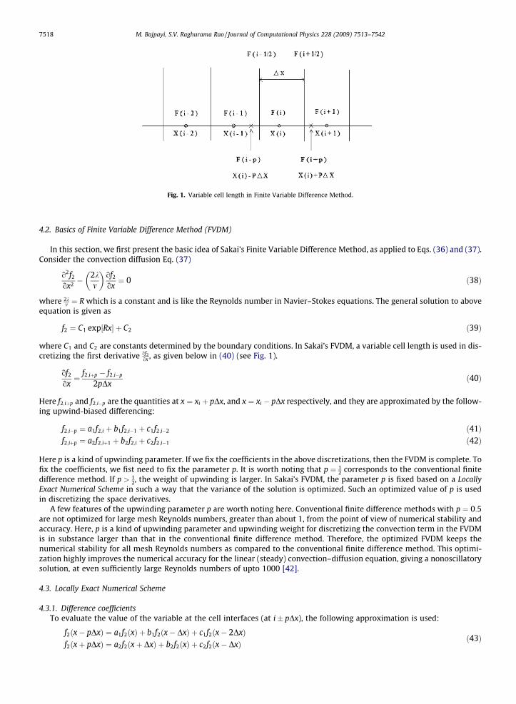
Fig. 1. Variable cell length in Finite Variable Difference Method.
7518 M. Bajpayi, S.V. Raghurama Rao / Journal of Computational Physics 228 (2009) 7513–7542
4.2. Basics of Finite Variable Difference Method (FVDM)
In this section, we first present the basic idea of Sakai’s Finite Variable Difference Method, as applied to Eqs. (36) and (37).Consider the convection diffusion Eq. (37)
o2f2
ox2 �2km
� �of2
ox¼ 0 ð38Þ
where 2km ¼ R which is a constant and is like the Reynolds number in Navier–Stokes equations. The general solution to above
equation is given as
f2 ¼ C1 exp½Rx� þ C2 ð39Þ
where C1 and C2 are constants determined by the boundary conditions. In Sakai’s FVDM, a variable cell length is used in dis-cretizing the first derivative of2
ox , as given below in (40) (see Fig. 1).
of2
ox¼ f2;iþp � f2;i�p
2pDxð40Þ
Here f2;iþp and f2;i�p are the quantities at x ¼ xi þ pDx, and x ¼ xi � pDx respectively, and they are approximated by the follow-ing upwind-biased differencing:
f2;i�p ¼ a1f2;i þ b1f2;i�1 þ c1f2;i�2 ð41Þf2;iþp ¼ a2f2;iþ1 þ b2f2;i þ c2f2;i�1 ð42Þ
Here p is a kind of upwinding parameter. If we fix the coefficients in the above discretizations, then the FVDM is complete. Tofix the coefficients, we fist need to fix the parameter p. It is worth noting that p ¼ 1
2 corresponds to the conventional finitedifference method. If p > 1
2, the weight of upwinding is larger. In Sakai’s FVDM, the parameter p is fixed based on a LocallyExact Numerical Scheme in such a way that the variance of the solution is optimized. Such an optimized value of p is usedin discretizing the space derivatives.
A few features of the upwinding parameter p are worth noting here. Conventional finite difference methods with p ¼ 0:5are not optimized for large mesh Reynolds numbers, greater than about 1, from the point of view of numerical stability andaccuracy. Here, p is a kind of upwinding parameter and upwinding weight for discretizing the convection term in the FVDMis in substance larger than that in the conventional finite difference method. Therefore, the optimized FVDM keeps thenumerical stability for all mesh Reynolds numbers as compared to the conventional finite difference method. This optimi-zation highly improves the numerical accuracy for the linear (steady) convection–diffusion equation, giving a nonoscillatorysolution, at even sufficiently large Reynolds numbers of upto 1000 [42].
4.3. Locally Exact Numerical Scheme
4.3.1. Difference coefficientsTo evaluate the value of the variable at the cell interfaces (at i� pDx), the following approximation is used:
f2ðx� pDxÞ ¼ a1f2ðxÞ þ b1f2ðx� DxÞ þ c1f2ðx� 2DxÞf2ðxþ pDxÞ ¼ a2f2ðxþ DxÞ þ b2f2ðxÞ þ c2f2ðx� DxÞ
ð43Þ
M. Bajpayi, S.V. Raghurama Rao / Journal of Computational Physics 228 (2009) 7513–7542 7519
Applying Taylor series expansion on both the sides of Eq. (43) and comparing coefficients of f2ðxÞ on both the sides we have
a1 þ b1 þ c1 ¼ 1 and a2 þ b2 þ c2 ¼ 1 ð44Þ
Following Sakai, we impose the condition that Eq. (43) should satisfy identically the exact solution of the convection–diffu-sion Eq. (39) for arbitrary values of C1 and C2. Assuming C1 ¼ 1 and C2 ¼ 0 we have
exp½Rxi�p� ¼ a1 exp½Rxi� þ b1 exp½Rxi�1� þ c1 exp½Rxi�2�exp½Rxiþp� ¼ a2 exp½Rxiþ1� þ b2 exp½Rxi� þ c2 exp½Rxi�1�
ð45Þ
We rewrite the above equation as
exp½Rxi�p� ¼ exp½ln a1 þ Rxi� þ exp½ln b1 þ Rxi�1� þ exp½ln c1 þ Rxi�2�exp½Rxiþp� ¼ exp½ln a2 þ Rxiþ1� þ exp½ln b2 þ Rxi� þ exp½ln c2 þ Rxi�1�
Applying exponential series expansion to the above equation and comparing the coefficients of R on both sides, we have
xi�p ¼ a1xi þ b1xi�1 þ c1xi�2
xiþp ¼ a2xiþ1 þ b2xi þ c2xi�1ð46Þ
Writing Eqs. (44)–(46) together, we get the following matrix of equations for the difference coefficients:
½M�a1
b1
c1
264375 ¼ 1
xi�p
exp½Rxi�p�
264375 ð47Þ
½N�a2
b2
c2
264375 ¼ 1
xiþp
exp½Rxiþp�
264375 ð48Þ
where
½M� ¼1 1 1xi xi�1 xi�2
exp½Rxi� exp½Rxi�1� exp½Rxi�2�
264375 ð49Þ
½N� ¼1 1 1
xiþ1 xi xi�1
exp½Rxiþ1� exp½Rxi� exp½Rxi�1�
264375 ð50Þ
If p is given in Eqs. (47) and (48), we can obtain the coefficients a1; b1; c1; a2; b2; c2 . Once these coefficients are available, theycan be used in the approximation (43). Sakai evaluated the value of p by minimizing the variance of the solution. This pro-cedure is explained for the equations considered here in the following subsections.
4.3.2. Characteristic equationConsider now Eqs. (36) and (37). Discretizing the convection terms in Eq. (37) and using Eqs. (40)–(42), together with
discretizing the diffusion terms with second order central differences, we obtain
f2;iþ1 � 2f 2;i þ f2;i�1
Dxð Þ2� R
f2;iþpDx � f2;i�pDx
2pDx¼ 0
or
f2;iþ1 � 2:f2;i þ f2;i�1�
� RDx2p
� �a2f2;iþ1 þ b2f2;i þ c2f2;i�1� � a1f2;i þ b1f2;i�1 þ c1f2;i�2� " #
¼ 0
Let RDx ¼ R0, which is similar to the mesh Reynolds number. Rearranging the above equation yields the following differenceequation:
Af2;iþ1 þ Bf2;i þ Cf2;i�1 þ Df2;i�2 ¼ 0 ð51Þ
where
A ¼ 1� R0
2p a2
B ¼ �½2þ R0
2p ðb2 � a1Þ�
C ¼ 1� R0
2p ðc2 � b1Þ
D ¼ R0
2p c1
ð52Þ
7520 M. Bajpayi, S.V. Raghurama Rao / Journal of Computational Physics 228 (2009) 7513–7542
Eq. (51) has an exact solution (see [24]) given by
f2;i ¼ aðZ1Þi þ bðZ2Þi þ cðZ3Þi ð53Þ
where a; b and c are constants determined by the boundary conditions. In Eq. (53), Z1; Z2 and Z3 are the roots of the char-acteristic equation given by
AZ3 þ BZ2 þ CZ þ D ¼ 0 ð54Þ
Since a1 þ b1 þ c1 ¼ 1 and a2 þ b2 þ c2 ¼ 1, from Eq. (52), we get the relation
Aþ Bþ C þ D ¼ � R0
2p
� �a2 þ b2 þ c2ð Þ � a1 þ b1 þ c1ð Þ½ � ¼ 0 ð55Þ
Hence Eq. (54) has a root Z1 ¼ 1 and can be factorized as
ðZ � 1Þ 1� R0
2p
� �a1
� �Z2 � 1þ R0
2p
� �ð1� c2 � a1Þ
� �Z � R0
2p
� �c1
� �¼ 0 ð56Þ
From this equation, we obtain the other two roots as
Z2 ¼1þ R0
2p
�ð1� c2 � a1Þ þ
ffiffiffiffiRp
2 1� R0
2p
�a2
h i ð57Þ
Z3 ¼1þ R0
2p
�ð1� c2 � a1Þ �
ffiffiffiffiRp
2 1� R0
2p
�a2
h i ð58Þ
where
R ¼ 1þ R0
2p
� �ð1� c2 � a1Þ
� �2
þ 4 1� R0
2p
� �a2
� �R0
2pc1 ð59Þ
4.3.3. Stability conditionTypically, the oscillations in the numerical solution occur because of the behaviour of the exact solution of the difference
(discretized) equations. Therefore, it is reasonable to study the behaviour of the exact solution of the difference equation (in-stead of the round-off errors), by inspecting the positivity of roots of the difference equation, since the presence of a negativeroot indicates oscillations in the solution [41]. Therefore, we inspect the positivity of the roots ðZ1; Z2; Z3Þ for determining thestability of the scheme. Thus, we impose the condition as
R P 0; Z1 P 0; Z2 P 0; Z3 P 0: ð60Þ
We numerically examine the dependence of characteristic roots on p (0:1 6 p 6 1) for 0:1 6 R0 6 1000. The first stability con-dition R P 0 is always fulfilled for any p and R0. Both Z2 and Z3 are positive for all p under consideration in the case of R0 ¼ 2,while in the case of R0 ¼ 10 an asymptote ðp ¼ paÞ for Z2 exists, and Z2 is negative for p > pa. The asymptote ðp ¼ paÞ for Z2
occurs when the denominator of Eq. (57) is zero. The equation to determine pa (for vanishing denominators in Eqs. (57) and(58)) is
1� R0
2pa
� �a2ðpa;R
0Þ ¼ 0 ð61Þ
where the notation a2ðpa;R0Þ is used, since the coefficient a2 involves p and R0 as parameters. When p approaches pa, the
numerator of Z3 approaches zero. Hence Z3 varies continuously even in the vicinity of p ¼ pa. A critical value R0c, where Z2
can be negative for R0 greater than R0c is given by Eq. (61) with pa ¼ 1:0, which is the maximum value of p. The equationto determine R0c is
1� R0c2
� �a2ð1:0;R0cÞ ¼ 0 ð62Þ
Solving Eq. (62) numerically results in R0c ¼ 2. Then we solve Eq. (61) for R0 > R0c and obtain the asymptote pa in terms of R0. Ifp exceeds pa; Z2 becomes negative and the solution of Eq. (53) oscillates. Therefore, to get numerical stability, p must be
ðfor R0 6 2Þ; 0 < p < 1;ðfor R0 > 2Þ; 0 < p < pa ¼ FðR0Þ
ð63Þ
M. Bajpayi, S.V. Raghurama Rao / Journal of Computational Physics 228 (2009) 7513–7542 7521
4.4. Variance of solution and optimum value of p
The variance r is defined as
r ¼ 1n
Xn
i¼1
½f2;i � f2;iðeÞðxiÞ�2 ð64Þ
Here n is the total mesh number, f2;i and f2;iðeÞðxiÞ represent the numerical solution and the exact solution at the mesh numberi, respectively. To evaluate r , we perform typical calculations in one dimensional geometry with the uniform mesh Dx ¼ 1
n, inwhich the total mesh number n and the computational lengths are 15 and 1, respectively. The boundary values at x ¼ 0 andx ¼ 1 are set as f2;ið0Þ ¼ 1 and f2;ið1Þ ¼ 0. We have to determine value of p (denoted by p0) which minimizes r. FollowingSakai, we tabulate the values of the variance for different possibilities and obtain the correlation equation of p0 with respectto R0 as
for 0 < R0 6 14�
; p0 ¼ G R0�
for 14 6 R0 6 20�
; p0 ¼ F R0� � 10�6 ð20� R0Þ=6
for 20 6 R0�
; p0 ¼ F R0�
ð65Þ
The functions GðR0Þ and FðR0Þ can be obtained from the tabulated values of the variance (see [41]). Similar analysis can bedone for Eq. (36), where R will be replaced by �R and f2 will be replaced by f1.4.5. Source term treatment, well-balancing and solution update
Let us now consider the equations to be solved in the convection–diffusion-source step: (31) and (32). To emphasize theconcept of a well-balancing, let us first drop the unsteady terms in Eqs. (31) and (32), to obtain
� oðkf1Þox ¼
o m2of1ox
� ox þ o m
2of2ox
� ox
oðkf2Þox ¼
o m2of2ox
� ox þ o m
2of1ox
� ox
ð66Þ
Integrating above equations with respect to x we obtain
�kf1 ¼ m2
of1ox þ m
2of2ox þ constant
kf2 ¼ m2
of2ox þ m
2of1ox þ constant
ð67Þ
Adding both the equations, we get
kðf2 � f1Þ ¼ mof1
oxþ m
of2
oxþ constant) v ¼ m
ouoxþ constant) gðuÞ ¼ gvðuÞ þ constantðunder relaxation limitÞ
) �gðuÞ þ gvðuÞ ¼ constant ð68Þ
A numerical scheme that preserves the above steady state solution exactly at the cell-interfaces requires�gðuiþpÞ þ gvðuiþpÞ ¼ constant; 8i ð69Þ
or approximately with a formal second order accuracy
�gðuiþpÞ þ gvðuiþpÞ ¼ constantþ OððDxÞ2Þ; 8i ð70Þ
Let us now consider the Finite Variable Difference Relaxation Scheme. Let h1 ¼ �kf1 and h2 ¼ kf2. Integrating Eqs. (31) and(32) over a finite volume ½xi�p; xiþp� and over a finite time interval ½tn; tnþ1�, we obtain
Z tnþ1tn
Z xiþp
xi�p
of1
otdxdt þ
Z tnþ1
tn
Z xiþp
xi�p
oh1
oxdxdt ¼
Z tnþ1
tn
Z xiþp
xi�p
m2
o
oxof1
ox
� �dxdt þ
Z tnþ1
tn
Z xiþp
xi�p
m2
o
oxof2
ox
� �dxdt ð71Þ
and
Z tnþ1tn
Z xiþp
xi�p
of2
otdxdt þ
Z tnþ1
tn
Z xiþp
xi�p
oh2
oxdxdt ¼
Z tnþ1
tn
Z xiþp
xi�p
m2
o
oxof2
ox
� �dxdt þ
Z tnþ1
tn
Z xiþp
xi�p
m2
o
oxof1
ox
� �dxdt ð72Þ
Thus, we obtain
�f nþ11;i ¼ �f n
1;i �Dt
2pDxhn
1;iþp � hn1;i�p
h iþ m
2Dt
2pDx
of n1;iþp
ox�
of n1;i�p
ox
" #þ m
2Dt
2pDx
of n2;iþp
ox�
of n2;i�p
ox
" #ð73Þ
and
�f nþ12;i ¼ �f n
2;i �Dt
2pDxhn
2;iþp � hn2;i�p
h iþ m
2Dt
2pDx
of n2;iþp
ox�
of n2;i�p
ox
" #þ m
2Dt
2pDx
of n1;iþp
ox�
of n1;i�p
ox
" #ð74Þ
7522 M. Bajpayi, S.V. Raghurama Rao / Journal of Computational Physics 228 (2009) 7513–7542
The cell integral averages are defined by
�f 1;i ¼1
2pDx
Z xiþp
xi�p
f1 dx ð75Þ
�f 2;i ¼1
2pDx
Z xiþp
xi�p
f2 dx ð76Þ
Writing partial derivative terms as linear combination of neighbouring cell values, we have
of1
ox
� �iþp
¼ a3f1;iþ1 þ b3f1;i þ c3f1;i�1 ð77Þ
of1
ox
� �i�p
¼ a4f1;i þ b3f1;i�1 þ c3f1;i�2 ð78Þ
Therefore, we obtain
of1
ox
� �xþpDx
¼ a3f1ðxþ DxÞ þ b3f1ðxÞ þ c3f1ðx� DxÞ
) of1
oxðxÞ ¼ a3f1ðxþ ð1� pÞDxÞ þ b3f1ðx� pDxÞ þ c3f1ðx� ðpþ 1ÞDxÞ ð79Þ
Applying Taylor series expansion on both sides and comparing the coefficients of f1ðxÞ; of1ðxÞox and o2 f1ðxÞ
ox2 and solving system ofthree equations, we obtain
a3 ¼2pþ 1
2Dx; b3 ¼
�2pDx
; c3 ¼1� 2p
Dxð80Þ
Similar analysis yields
a4 ¼3� 2p
2Dx; b4 ¼
2ðp� 1ÞDx
; c3 ¼1� 2p
2Dxð81Þ
In the same manner of2ox
�iþp
and of2ox
�i�p
can be evaluated. Note that h1 þ h2 ¼ kðf2 � f1Þ ¼ v ¼ gðuÞ (under relaxation limit).
We can get the updating of the solution as
unþ1i ¼ f nþ1
1;i þ f nþ12;i ð82Þ
Under steady state conditions, Eqs. (73) and (74) become
� ½hn1;iþp � hn
1;i�p� þm2
of n1;iþp
ox�
of n1;i�p
ox
" #þ m
2of n
2;iþp
ox�
of n2;i�p
ox
" #¼ 0 ð83Þ
� ½hn2;iþp � hn
2;i�p� þm2
of n2;iþp
ox�
of n2;i�p
ox
" #þ m
2of n
1;iþp
ox�
of n1;i�p
ox
" #¼ 0 ð84Þ
Adding the above two equations, we obtain
� kf n2;iþp � kf n
1;iþp
h iþ m
oðf n1;iþp þ f n
2;iþpÞox
¼ �½kf n2;i�p � kf n
1;i�p� þ moðf n
1;i�p þ f n2;i�pÞ
oxð85Þ
) �gðuniþpÞ þ gvðun
iþpÞ ¼ �gðuni�pÞ þ gvðun
i�pÞ ðunder relaxation limitÞ ð86Þ
Hence this scheme is well balanced.
5. Finite Variable Difference Relaxation Scheme for 2D nonlinear conservation laws
As the relaxation system given by Jin and Xin is not diagonalizable in multi-dimensions, Aregba-Driollet and Natalini gen-eralized the discrete Boltzmann equation in 1-D to multi-dimensions to obtain a multi-dimensional relaxation system as
ofotþXD
k¼1
Kkofoxk¼ 1�½F � f � ð87Þ
For the multi-dimensional diagonal relaxation system, the local Maxwellians are defined by
FDþ1 ¼1D
uþ 1k
XD
k¼1
gkðuÞ" #
Fi ¼ �1k
giðuÞ þ FDþ1; ði ¼ 1; :::::;DÞ ð88Þ
M. Bajpayi, S.V. Raghurama Rao / Journal of Computational Physics 228 (2009) 7513–7542 7523
The 2-D discrete Boltzmann equation is given by
ofotþK1
ofoxþK2
ofoy¼ 1�½F � f � ð89Þ
where
K1 ¼�k 0 00 0 00 0 k
24 35 ð90Þ
and
K2 ¼0 0 00 �k 00 0 k
24 35 ð91Þ
The local Maxwellians are defined by
F ¼F1
F2
F3
264375 ¼
u3� 2
3k g1ðuÞ þ 13k g2ðuÞ
u3þ 1
3k g1ðuÞ � 23k g2ðuÞ
u3þ 1
3k g1ðuÞ þ 13k g2ðuÞ
264375 ð92Þ
Expanding Eqs. (89) leads to the following equations:
of1ot � k of1
ox ¼ 1� ½F1 � f1�
of2ot � k of2
oy ¼ 1� ½F2 � f2�
of3ot þ k of3
ox þ k of3oy ¼ 1
� ½F3 � f3�ð93Þ
where u ¼ f1 þ f2 þ f3; g1ðuÞ ¼ kðf3 � f1Þ and g2 ¼ kðf3 � f2Þ:Consider 2-D viscous Burgers equation
ouotþ og1ðuÞ
oxþ og2ðuÞ
oy¼ og1vðuÞ
oxþ og2vðuÞ
oyð94Þ
where g1v ðuÞ ¼ m ouox and g2v ¼ m ou
oy. Under relaxation approximation, as �! 0; f ¼ F. In analogy with the 1-D case, we intro-duce viscous terms in the discrete velocity Boltzmann equation in 2-D and utilize the following equations in the convec-tion–diffusion-source step of a 2-D relaxation system.
of1
ot� k
of1
ox¼ m
o2f1
ox2 þ mo2f2
ox2
of2
ot� k
of2
oy¼ m
o2f2
oy2 þ mo2f1
oy2
of3
otþ k
of3
oxþ k
of3
oy¼ m
o2f3
ox2 þ mo2f3
oy2 ð95Þ
Source terms in first two equations in the relaxation system (95) are treated using Jin’s well-balanced scheme [23]. Note thatthe last equation contains no source terms. Integrating equations (95) over a finite volume with an area defined by½xi�p; xiþp�½yj�p; yjþp� (where p is a kind of upwind parameter) and over a finite time interval ½tn; tnþ1�, we obtain, after a littlealgebraic manipulation, the following expressions.
�f nþ11;i;j ¼�f n
1;i;jþDt
2pDx½kf n
1;iþp;j�kf n1;i�p;j�þm
Dt2pDx
of n1;iþp;j
ox�
of n1;i�p;j
ox
" #þm
Dt2pDx
of n2;iþp;j
ox�
of n2;i�p;j
ox
" #ð96Þ
�f nþ12;i;j ¼�f n
2;i;jþDt
2pDy½kf n
2;i;jþp�kf n2;i;j�p�þm
Dt2pDy
of n2;i;jþp
oy�
of n2;i;j�p
oy
" #þm
Dt2pDy
of n1;i;jþp
oy�
of n1;i;j�p
oy
" #ð97Þ
�f nþ13;i;j ¼�f n
3;i;j�Dt
2pDx½kf n
3;iþp;j�kf n3;i�p;j��
Dt2pDy
½kf n3;i;jþp�kf n
3;i;j�p�þmDt
2pDx
of n3;iþp;j
ox�
of n3;i�p;j
ox
" #þm
Dt2pDy
of n3;i;jþp
oy�
of n3;i;j�p
oy
" #ð98Þ
The solution can be recovered as
unþ1i;j ¼ f nþ1
1;i;j þ f nþ12;i;j þ f nþ1
3;i;j ð99Þ
The cell interface fluxes are evaluated as in the 1-D case in each direction. The Finite Variable Difference Relaxation scheme,which is second order accurate, can yield mild wiggles near shocks, in the unsteady case. A simple minmax limiter is used tosuppress the spurious oscillations produced by the second order scheme, near the discontinuities.
7524 M. Bajpayi, S.V. Raghurama Rao / Journal of Computational Physics 228 (2009) 7513–7542
6. Extension of Finite Variable Difference Relaxation Scheme to shallow water equations
In this section, the Finite Variable Difference Relaxation Scheme is extended to the shallow water equations. Consider the1-D shallow water equations, given by
ohotþ o huð Þ
ox¼ 0 ð100Þ
o huð Þotþ
o hu2 þ 12 gh2
�ox
¼ �ghoBðxÞoxþ m
o
oxh
ouox
� �ð101Þ
Since the Finite Variable Difference Method of Sakai is designed for convection–diffusion equations, we first introduce a fic-titious viscosity term in the first equation of the above system (100) and take the value of the coefficient of fictitious viscosity(mf ) to be a very low value, close to zero. With the fictitious viscosity term, the system can be written as
ohotþ oðhuÞ
ox¼ mf
o
oxohox
� �ð102Þ
oðhuÞotþ
o hu2 þ 12 gh2
�ox
¼ �ghoBðxÞoxþ m
o
oxh
ouox
� �ð103Þ
The above system of equations can be written as
oUotþ oG
ox¼ SðUÞ ð104Þ
where
U ¼h
hu
� �; G ¼
hu
hu2 þ 12 gh2
" #ð105Þ
and
SðUÞ ¼mf
oox
ohox
� �gh oBðxÞ
ox þ m oox h ou
ox
� " #ð106Þ
We first introduce a convection–gravity splitting as
G ¼ Gc þ Gg ð107Þ
where
Gc ¼huhu2
� �and Gg ¼
012 gh2
" #ð108Þ
are the convective flux and the gravity flux respectively. Since the gravity essentially represents a force, we treat the gravityflux as a source term and include it in SðUÞ. With this modification, the 1-D shallow water equations are given by
oUotþ oGc
ox¼ eSðUÞ ð109Þ
where the modified source term which includes the gravity flux is now given by
eSðUÞ ¼ mfoox
ohox
� � o
ox12 gh2 �
� gh oBox þ m o
ox h ouox
� 24 35 ð110Þ
A relaxation system for the above system of equations can now be introduced as
oUotþ oV
ox¼ eSðUÞ ð111Þ
oVotþ D
oUox¼ �1
�V � Gc �
; �! 0 ð112Þ
where D is a diagonal matrix, defined by
D ¼k2
1 0
0 k22
" #ð113Þ
For simplicity, let us assume k21 ¼ �k2
2 ¼ k2 and the value of k is taken to the be the global maximum of the absolute values ofthe eigenvalues of the flux Jacobian matrix Ac ¼ oGc
oU . The quasi-linear form of the relaxation system is given by
M. Bajpayi, S.V. Raghurama Rao / Journal of Computational Physics 228 (2009) 7513–7542 7525
oQotþ A
oQox¼ H ð114Þ
where
Q ¼U
V
� �; A ¼
0 1D 0
� �and H ¼
eSðUÞ� 1� V � Gc� " #
ð115Þ
Since the convection terms on the left hand side of the relaxation system represent the hyperbolic part, we can introducecharacteristic variables and decouple the system (as in Section 2) to obtain the following two equations:
of1
ot� k
of1
ox¼ 1
2eSðUÞ þ 1
2k�V � Gc �
ð116Þ
of2
otþ k
of2
ox¼ 1
2eSðUÞ � 1
2k�V � Gc �
ð117Þ
where
f ¼f1
f2
� �¼
12 U � 1
2k V12 U þ 1
2k V
" #ð118Þ
Introducing the new variable F as
F ¼F1
F2
� �¼
12 U � 1
2k Gc
12 U þ 1
2k Gc
" #ð119Þ
and using the definition U ¼ f1 þ f2, we obtain
of1
ot� k
of1
ox¼ 1
2eSðUÞ � 1
�f1 � F1½ � ð120Þ
of2
otþ k
of2
ox¼ 1
2eSðUÞ � 1
�f2 � F2½ � ð121Þ
where f1 and f2 are vectors with two components each for 1-D case. Note that each of f1 and f2 contains two components.
f1 ¼f1;1
f1;2
� �and f 2 ¼
f2;1
f2;2
� �ð122Þ
Therefore, after substituting values of eSðUÞ, we get following set of decoupled equations:
of1;1
ot� k
of1;1
ox¼ 1
2mf
o
oxohox
� �� 1�
f1;1 � F1;1½ � ð123Þ
of1;2
ot� k
of1;2
ox¼ 1
2� o
ox12
gh2� �
� ghoBoxþ m
o
oxh
ouox
� �� �� 1�
f1;2 � F1;2½ � ð124Þ
of2;1
otþ k
of2;1
ox¼ 1
2mf
o
oxohox
� �� 1�
f2;1 � F2;1½ � ð125Þ
of2;2
otþ k
of2;2
ox¼ 1
2� o
ox12
gh2� �
� ghoBoxþ m
o
oxh
ouox
� �� �� 1�
f2;2 � F2;2½ � ð126Þ
Sakai’s Finite Variable Difference Method is applied to the aforementioned system of equations by converting the fictitiousviscous term and viscous term (corresponding to mass and momentum conservation equations respectively) in terms ofcharacteristic variables. From U ¼ f1 þ f2, we get
h ¼ f1;1 þ f2;1 and hu ¼ f1;2 þ f2;2
Therefore
mfo
oxohox
� �¼ mf
o
oxo f1;1 þ f2;1ð Þ
ox
� �¼ mf
o2f1;1
ox2 þ mfo2f2;1
ox2 ð127Þ
and
o
oxðhuÞ ¼ of1;2
oxþ of2;2
ox
or houoxþ u
ohox¼ of1;2
oxþ of2;2
ox
7526 M. Bajpayi, S.V. Raghurama Rao / Journal of Computational Physics 228 (2009) 7513–7542
Differentiating both sides with respect to x and multiplying by m we obtain
mo
oxh
ouox
� �þ m
o
oxu
ohox
� �¼ m
o2f1;2
ox2 þ mo2f2;2
ox2
or mo
oxh
ouox
� �¼ m
o2f1;2
ox2 þ mo2f2;2
ox2 � mo
oxu
ohox
� �or m
o
oxh
ouox
� �¼ m
o2f1;2
ox2 þ mo2f2;2
ox2 � mo
oxU2
U1
o
oxf1;1 þ f2;1ð Þ
� �or m
o
oxh
ouox
� �¼ m
o2f1;2
ox2 þ mo2f2;2
ox2 � mo
oxU2
U1
of1;1
ox
� �� m
o
oxU2
U1
of2;1
ox
� �ð128Þ
where
U2
U1¼ u ¼ hu
h¼ f1;2 þ f2;2
f1;1 þ f2;1ð129Þ
Substituting (127) in (123), (125) and (128) in (124), (126), we obtain
of1;1
ot� k
of1;1
ox¼ 1
2mf
o2f1;1
ox2 þ12mf
o2f2;1
ox2 �1�
f1;1 � F1;1½ � ð130Þ
of1;2
ot� k
of1;2
ox¼ 1
2m
o2f1;2
ox2 þ12m
o2f2;2
ox2 �12m
o
oxU2
U1
of1;1
ox
� �� 1
2m
o
oxU2
U1
of2;1
ox
� �þ 1
2� o
ox12
g f1;1 þ f2;1ð Þ2� �
� g f1;1 þ f2;1ð Þ oBox
� �� 1�
f1;2 � F1;2½ � ð131Þ
of2;1
otþ k
of2;1
ox¼ 1
2mf
o2f1;1
ox2 þ12mf
o2f2;1
ox2 �1�
f2;1 � F2;1½ � ð132Þ
of2;2
otþ k
of2;2
ox¼ 1
2m
o2f1;2
ox2 þ12m
o2f2;2
ox2 �12m
o
oxU2
U1
of1;1
ox
� �� 1
2m
o
oxU2
U1
of2;1
ox
� �þ 1
2� o
ox12
g f1;1 þ f2;1ð Þ2� �
� g f1;1 þ f2;1ð Þ oBox
� �� 1�
f2;2 � F2;2½ � ð133Þ
Defining ~mf ¼ 12 mf and ~m ¼ 1
2 m, we can rewrite Eqs. (130) to (133) as
of1;1
ot� k
of1;1
ox¼ ~mf
o2f1;1
ox2 �1�
f1;1 � F1;1½ � þ S1;1 ð134Þ
of1;2
ot� k
of1;2
ox¼ ~mf
o2f1;2
ox2 �1�
f1;2 � F1;2½ � þ S1;2 ð135Þ
of2;1
otþ k
of2;1
ox¼ ~mf
o2f2;1
ox2 �1�
f2;1 � F2;1½ � þ S2;1 ð136Þ
of2;2
otþ k
of2;2
ox¼ ~mf
o2f2;2
ox2 �1�
f2;2 � F2;2½ � þ S2;2 ð137Þ
where the source terms in the above equations are given by
S1;1 ¼ ~mfo2f2;1
ox2
S1;2 ¼ ~mo2f2;2
ox2 � ~mo
oxU2
U1
of1;1
ox
� �� ~m
o
oxU2
U1
of2;1
ox
� �� 1
2o
ox12
g f1;1 þ f2;1ð Þ2� �
� 12
g f1;1 þ f2;1ð Þ oBox
ð138Þ
S2;1 ¼ ~mfo2f1;1
ox2
S2;2 ¼ ~mo2f1;2
ox2 � ~mo
oxU2
U1
of1;1
ox
� �� ~m
o
oxU2
U1
of2;1
ox
� �� 1
2o
ox12
g f1;1 þ f2;1ð Þ2� �
� 12
g f1;1 þ f2;1ð Þ oBox
Note that each of Eqs. (134), (137) is a convection–diffusion equation together with a relaxation term and a source term. Weapply the Finite Variable Difference Method of Sakai to each of these convection–diffusion equations, treating the sourceterms using the strategy introduced by Jin (as in Section 4). Note also that the final convection–diffusion equations usedare linear while source terms in both the equations are nonlinear and both FVDM of Sakai and Jin’s strategy for discretizingthe source term are well-suited for these terms, respectively. The value of fictitious viscosity coefficient in modified massconservation equation is taken as mf ¼ 10�4. For the case of 2-D shallow water equations, the convection–gravity splittingmethod is similar to the 1-D case as explained before. Together with this strategy of treating the gravity terms as sourceterms, the 2-D discrete velocity Boltzmann equation (introduced in Section 5) is utilized as the relaxation system and theFVDM for the resulting 2-D convection–diffusion equations is as given in Section 5.
M. Bajpayi, S.V. Raghurama Rao / Journal of Computational Physics 228 (2009) 7513–7542 7527
7. Numerical experiments
This new algorithm, Finite Variable Difference Relaxation Scheme, is tested on several benchmark problems for inviscidand viscous Burgers equations and for shallow water equations both in one and two dimensions.
7.1. 1-D inviscid Burgers equation test case
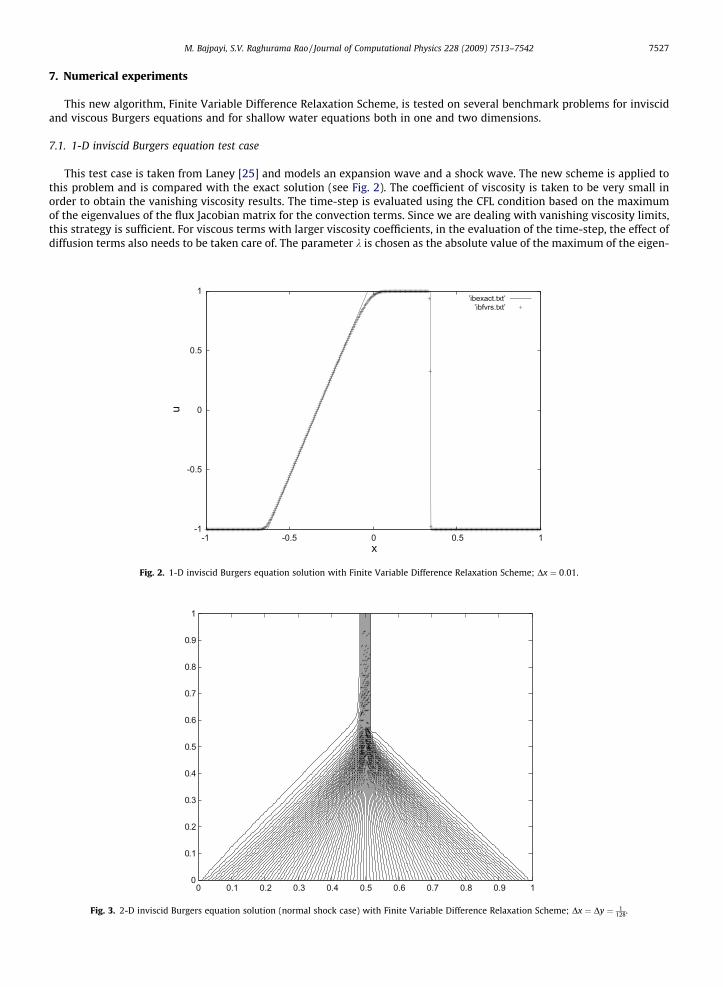
This test case is taken from Laney [25] and models an expansion wave and a shock wave. The new scheme is applied tothis problem and is compared with the exact solution (see Fig. 2). The coefficient of viscosity is taken to be very small inorder to obtain the vanishing viscosity results. The time-step is evaluated using the CFL condition based on the maximumof the eigenvalues of the flux Jacobian matrix for the convection terms. Since we are dealing with vanishing viscosity limits,this strategy is sufficient. For viscous terms with larger viscosity coefficients, in the evaluation of the time-step, the effect ofdiffusion terms also needs to be taken care of. The parameter k is chosen as the absolute value of the maximum of the eigen-
-1
-0.5
0
0.5
1
-1 -0.5 0 0.5 1
u
x
’ibexact.txt’’ibfvrs.txt’
Fig. 2. 1-D inviscid Burgers equation solution with Finite Variable Difference Relaxation Scheme; Dx ¼ 0:01.
0 0.1 0.2 0.3 0.4 0.5 0.6 0.7 0.8 0.9 10
0.1
0.2
0.3
0.4
0.5
0.6
0.7
0.8
0.9
1
Fig. 3. 2-D inviscid Burgers equation solution (normal shock case) with Finite Variable Difference Relaxation Scheme; Dx ¼ Dy ¼ 1128.
7528 M. Bajpayi, S.V. Raghurama Rao / Journal of Computational Physics 228 (2009) 7513–7542
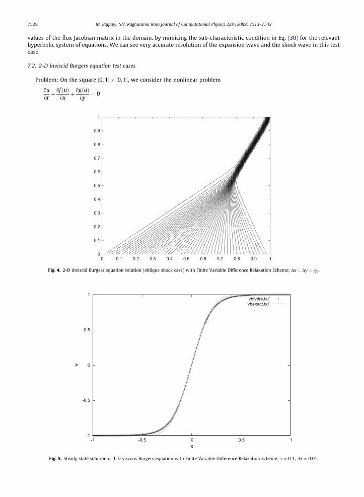
values of the flux Jacobian matrix in the domain, by mimicing the sub-characteristic condition in Eq. (30) for the relevanthyperbolic system of equations. We can see very accurate resolution of the expansion wave and the shock wave in this testcase.
7.2. 2-D inviscid Burgers equation test cases
Problem: On the square ½0;1� � ½0;1�, we consider the nonlinear problem
ouotþ of ðuÞ
oxþ ogðuÞ
oy¼ 0
0 0.1 0.2 0.3 0.4 0.5 0.6 0.7 0.8 0.9 10
0.1
0.2
0.3
0.4
0.5
0.6
0.7
0.8
0.9
1
Fig. 4. 2-D inviscid Burgers equation solution (oblique shock case) with Finite Variable Difference Relaxation Scheme; Dx ¼ Dy ¼ 1128.
-1
-0.5
0
0.5
1
-1 -0.5 0 0.5 1
v
x
’vbfvdrs.txt’’vbexact.txt’
Fig. 5. Steady state solution of 1-D viscous Burgers equation with Finite Variable Difference Relaxation Scheme; m ¼ 0:1; Dx ¼ 0:01.
M. Bajpayi, S.V. Raghurama Rao / Journal of Computational Physics 228 (2009) 7513–7542 7529
where
f ðuÞ ¼ 12
u2; gðuÞ ¼ u
Two sets of boundary conditions have been considered:Case 1. Boundary conditions:
uð0; yÞ ¼ 1; 0 < y < 1uð1; yÞ ¼ �1; 0 < y < 1uðx;0Þ ¼ 1� 2x; 0 < x < 1
ð139Þ
Fig. 6. 2-D viscous Burgers equation test case (left) initial condition and (right) steady state solution; Dx ¼ Dy ¼ 0:02.
1
1.5
2
2.5
3
-6 -4 -2 0 2 4 6
h
x
’1dswe_h_exact_t=0.5.txt’’1dswe_h_fvdrs_t=0.5.txt’
Fig. 7. Solution of depth h (+) at t ¼ 0:5 using FVDRS with Dx ¼ 0:01; solid line: exact solution.
7530 M. Bajpayi, S.V. Raghurama Rao / Journal of Computational Physics 228 (2009) 7513–7542
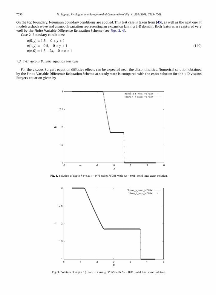
On the top boundary, Neumann boundary conditions are applied. This test case is taken from [45], as well as the next one. Itmodels a shock wave and a smooth variation representing an expansion fan in a 2-D domain. Both features are captured verywell by the Finite Variable Difference Relaxation Scheme (see Figs. 3, 4).
Case 2. Boundary conditions:
uð0; yÞ ¼ 1:5; 0 < y < 1uð1; yÞ ¼ �0:5; 0 < y < 1uðx; 0Þ ¼ 1:5� 2x; 0 < x < 1
ð140Þ
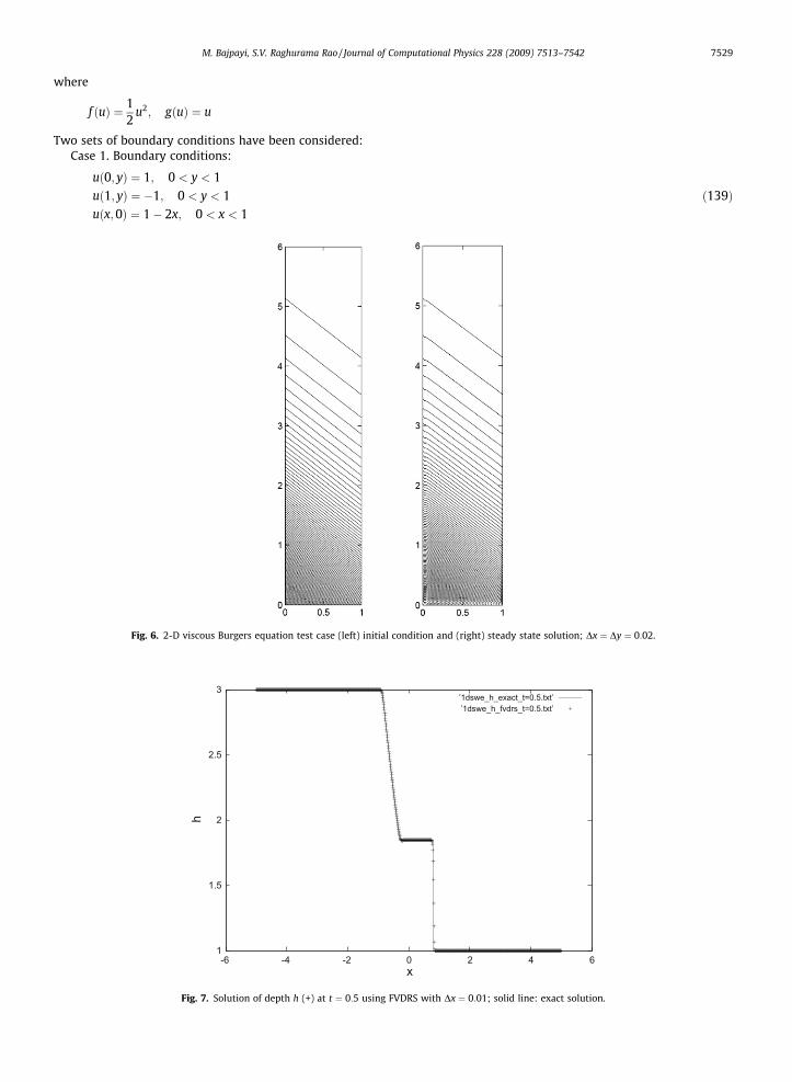
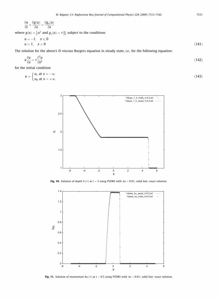
7.3. 1-D viscous Burgers equation test case
For the viscous Burgers equation diffusive effects can be expected near the discontinuities. Numerical solution obtainedby the Finite Variable Difference Relaxation Scheme at steady state is compared with the exact solution for the 1-D viscousBurgers equation given by
1
1.5
2
2.5
3
-6 -4 -2 0 2 4 6
h
x
’1dswe_1_h_fvdrs_t=0.75.txt’’1dswe_1_h_exact_t=0.75.txt’
Fig. 8. Solution of depth h (+) at t ¼ 0:75 using FVDRS with Dx ¼ 0:01; solid line: exact solution.
1
1.5
2
2.5
3
-6 -4 -2 0 2 4 6
h
x
’1dswe_h_exact_t=2.0.txt’’1dswe_h_fvdrs_t=2.0.txt’
Fig. 9. Solution of depth h (+) at t ¼ 2 using FVDRS with Dx ¼ 0:01; solid line: exact solution.
M. Bajpayi, S.V. Raghurama Rao / Journal of Computational Physics 228 (2009) 7513–7542 7531
ouotþ ogðuÞ
ox¼ ogvðuÞ
ox
where gðuÞ ¼ 12 u2 and gvðuÞ ¼ m ou
ox, subject to the conditions
u ¼ �1; x 6 0u ¼ 1; x > 0 ð141Þ
The solution for the above1-D viscous Burgers equation in steady state, i.e., for the following equation:
uouox¼ m
o2uox2 ð142Þ
for the initial condition
u ¼uL at x ¼ �1uR at x ¼ þ1
�ð143Þ
1
1.5
2
2.5
3
-6 -4 -2 0 2 4 6
h
x
’1dswe_1_h_fvdrs_t=3.0.txt’’1dswe_1_h_exact_t=3.0.txt’
Fig. 10. Solution of depth h (+) at t ¼ 3 using FVDRS with Dx ¼ 0:01; solid line: exact solution.
0
0.2
0.4
0.6
0.8
1
1.2
1.4
-6 -4 -2 0 2 4 6
hu
x
’1dswe_hu_exact_t=0.5.txt’’1dswe_hu_fvdrs_t=0.5.txt’
Fig. 11. Solution of momentum hu (+) at t ¼ 0:5 using FVDRS with Dx ¼ 0:01; solid line: exact solution.
7532 M. Bajpayi, S.V. Raghurama Rao / Journal of Computational Physics 228 (2009) 7513–7542
is given by [9]
u ¼ 12
uL þ uRð Þ � uL � uRð Þ tanhx uL � uRð Þ
4m
� �� �ð144Þ
The results show good resolution of the solution with very little numerical dissipation as compared to the exact solution (seeFig. 5).
7.4. 2-D viscous Burgers equation test case
This test case is taken from [30]. We consider viscous Burgers equation as
ouot¼ �u
ouoxþ ou
oy
� �þ 0:01
o2uox2 þ
o2uoy2
!
0
0.2
0.4
0.6
0.8
1
1.2
1.4
-6 -4 -2 0 2 4 6
hu
x
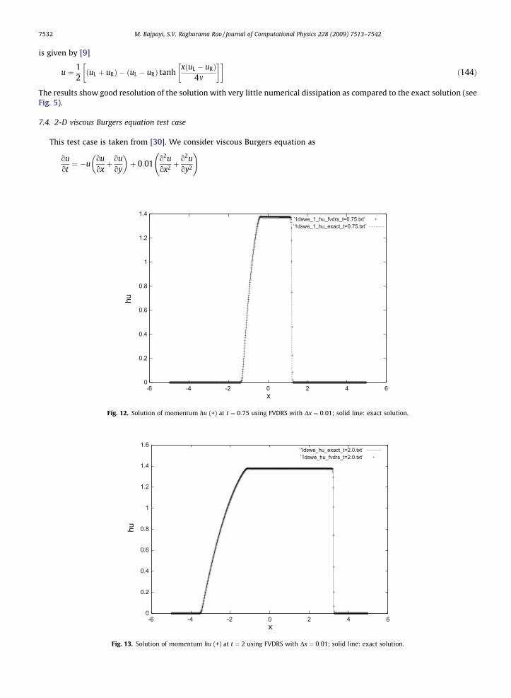
’1dswe_1_hu_fvdrs_t=0.75.txt’’1dswe_1_hu_exact_t=0.75.txt’
Fig. 12. Solution of momentum hu (+) at t ¼ 0:75 using FVDRS with Dx ¼ 0:01; solid line: exact solution.
0
0.2
0.4
0.6
0.8
1
1.2
1.4
1.6
-6 -4 -2 0 2 4 6
hu
x
’1dswe_hu_exact_t=2.0.txt’’1dswe_hu_fvdrs_t=2.0.txt’
Fig. 13. Solution of momentum hu (+) at t ¼ 2 using FVDRS with Dx ¼ 0:01; solid line: exact solution.
M. Bajpayi, S.V. Raghurama Rao / Journal of Computational Physics 228 (2009) 7513–7542 7533
We take the initial and boundary conditions of the form
1þ expðxþ y� tÞ�1 ð145Þ
With these initial conditions, the solution is a straight line wave (u is constant for x ¼ �y) moving in the direction h ¼ p4. The
numerical solution obtained is well in agreement with the exact solution (see Fig. 6).
7.5. 1-D shallow water equations test cases
Consider ‘‘Viscous Saint-Venant system” for shallow water equations with topography neglecting bed friction [33], as
ohotþ oðhuÞ
ox¼ 0 ð146Þ
ohuotþ
o hu2 �ox
þo 1
2 gh2 �
ox¼ �gh
oBðxÞoxþ m
o
oxh
ouox
� �ð147Þ
0
0.2
0.4
0.6
0.8
1
1.2
1.4
1.6
-6 -4 -2 0 2 4 6
hu
x
’1dswe_1_hu_fvdrs_t=3.0.txt’’1dswe_1_hu_exact_t=3.0.txt’
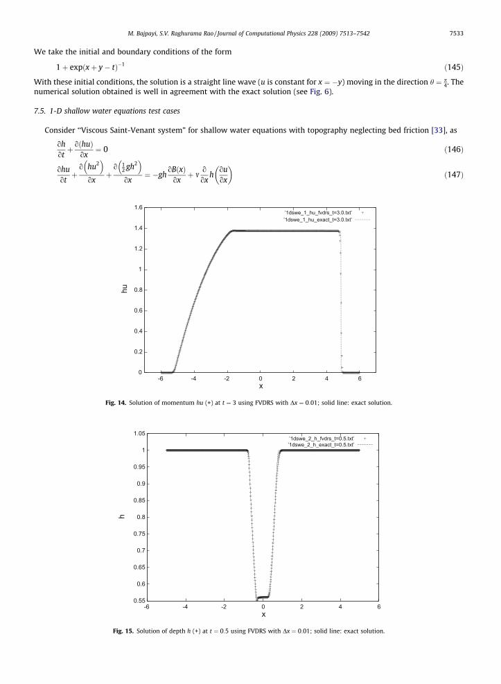
Fig. 14. Solution of momentum hu (+) at t ¼ 3 using FVDRS with Dx ¼ 0:01; solid line: exact solution.
0.55
0.6
0.65
0.7
0.75
0.8
0.85
0.9
0.95
1
1.05
-6 -4 -2 0 2 4 6
h
x
’1dswe_2_h_fvdrs_t=0.5.txt’’1dswe_2_h_exact_t=0.5.txt’
Fig. 15. Solution of depth h (+) at t ¼ 0:5 using FVDRS with Dx ¼ 0:01; solid line: exact solution.
7534 M. Bajpayi, S.V. Raghurama Rao / Journal of Computational Physics 228 (2009) 7513–7542
Here, h is depth of the water, u is the mean velocity, g is the gravitational constant, m is the coefficient of viscosity and BðxÞ isthe bottom elevation. The Finite Variable Difference Relaxation Scheme (FVDRS) presented in Section 6 is applied under van-ishing viscosity limits for several benchmark problems. Spurious oscillations in the vicinity of the shocks are suppressed byusing a minmod limiter. The 1-d shallow water equations are tested on the following bench-mark problems.
7.5.1. Dam break flowThis test case is taken from [27]. Consider the shallow water equations with the piecewise constant initial data as
hðx;0Þ ¼ 3; uðx;0Þ ¼ 0; for x 6 0 ð148Þhðx;0Þ ¼ 1; uðx;0Þ ¼ 0; for x > 0 ð149Þ
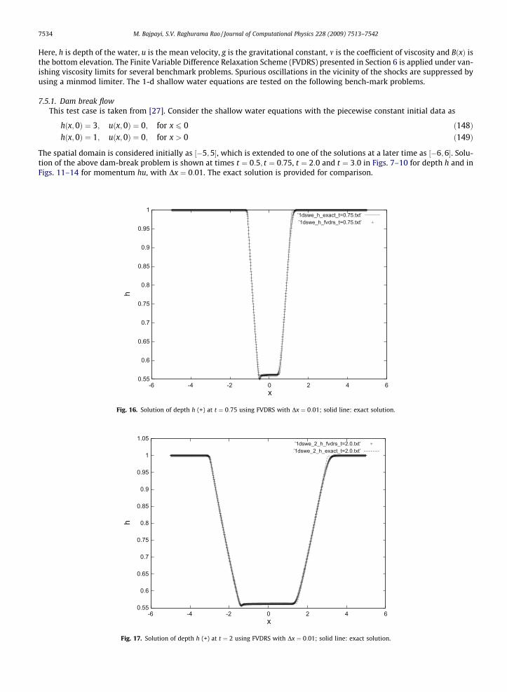
The spatial domain is considered initially as ½�5;5�, which is extended to one of the solutions at a later time as ½�6;6�. Solu-tion of the above dam-break problem is shown at times t ¼ 0:5; t ¼ 0:75, t ¼ 2:0 and t ¼ 3:0 in Figs. 7–10 for depth h and inFigs. 11–14 for momentum hu, with Dx ¼ 0:01. The exact solution is provided for comparison.
0.55
0.6
0.65
0.7
0.75
0.8
0.85
0.9
0.95
1
-6 -4 -2 0 2 4 6
h
x
’1dswe_h_exact_t=0.75.txt’’1dswe_h_fvdrs_t=0.75.txt’
Fig. 16. Solution of depth h (+) at t ¼ 0:75 using FVDRS with Dx ¼ 0:01; solid line: exact solution.
0.55
0.6
0.65
0.7
0.75
0.8
0.85
0.9
0.95
1
1.05
-6 -4 -2 0 2 4 6
h
x
’1dswe_2_h_fvdrs_t=2.0.txt’’1dswe_2_h_exact_t=2.0.txt’
Fig. 17. Solution of depth h (+) at t ¼ 2 using FVDRS with Dx ¼ 0:01; solid line: exact solution.
M. Bajpayi, S.V. Raghurama Rao / Journal of Computational Physics 228 (2009) 7513–7542 7535
7.5.2. Rarefaction riemann problemThis test case is taken from [27]. Consider the Riemann problem for the shallow water equations with data given as
follows:
hðx;0Þ ¼ 1:0; uðx; 0Þ ¼ �0:5; for x 6 0 ð150Þhðx;0Þ ¼ 1:0; uðx; 0Þ ¼ 0:5; for x > 0 ð151Þ
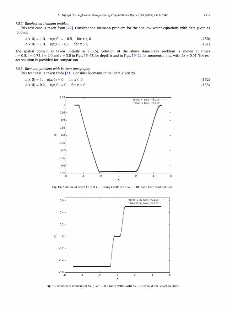
The spatial domain is taken initially as ½�5;5�. Solution of the above dam-break problem is shown at timest ¼ 0:5; t ¼ 0:75; t ¼ 2:0 and t ¼ 3:0 in Figs. 15–18 for depth h and in Figs. 19–22 for momentum hu, with Dx ¼ 0:01. The ex-act solution is provided for comparison.
7.5.3. Riemann problem with bottom topographyThis test case is taken from [23]. Consider Riemann initial data given by
hðx;0Þ ¼ 1; uðx; 0Þ ¼ 0; for x 6 0 ð152Þhðx;0Þ ¼ 0:2; uðx; 0Þ ¼ 0; for x > 0 ð153Þ
0.55
0.6
0.65
0.7
0.75
0.8
0.85
0.9
0.95
1
1.05
-6 -4 -2 0 2 4 6
h
x
’1dswe_h_exact_t=3.0.txt’’1dswe_h_fvdrs_t=3.0.txt’
Fig. 18. Solution of depth h (+) at t ¼ 3 using FVDRS with Dx ¼ 0:01; solid line: exact solution.
-0.6
-0.4
-0.2
0
0.2
0.4
0.6
-6 -4 -2 0 2 4 6
hu
x
’1dswe_2_hu_fvdrs_t=0.5.txt’’1dswe_2_hu_exact_t=0.5.txt’
Fig. 19. Solution of momentum hu (+) at t ¼ 0:5 using FVDRS with Dx ¼ 0:01; solid line: exact solution.
-0.6
-0.4
-0.2
0
0.2
0.4
0.6
-6 -4 -2 0 2 4 6
hu
x
’1dswe_hu_exact_t=0.75.txt’’1dswe_hu_fvdrs_t=0.75.txt’
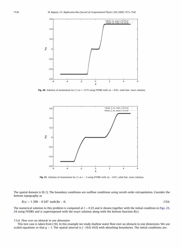
Fig. 20. Solution of momentum hu (+) at t ¼ 0:75 using FVDRS with Dx ¼ 0:01; solid line: exact solution.
-0.6
-0.4
-0.2
0
0.2
0.4
0.6
-6 -4 -2 0 2 4 6
hu
x
’1dswe_2_hu_fvdrs_t=2.0.txt’’1dswe_2_hu_exact_t=2.0.txt’
Fig. 21. Solution of momentum hu (+) at t ¼ 2 using FVDRS with Dx ¼ 0:01; solid line: exact solution.
7536 M. Bajpayi, S.V. Raghurama Rao / Journal of Computational Physics 228 (2009) 7513–7542
The spatial domain is [0,1]. The boundary conditions are outflow conditions using zeroth order extrapolation. Consider thebottom topography as
BðxÞ ¼ 1:398� 0:347 tanhð8x� 4Þ ð154Þ
The numerical solution to this problem is computed at t ¼ 0:25 and is shown together with the initial condition in Figs. 23,24 using FVDRS and is superimposed with the exact solution along with the bottom function B(x).
7.5.4. Flow over an obstacle in one dimensionThis test case is taken from [18]. In this example we study shallow water flow over an obstacle in one dimension. We use
scaled equations so that g ¼ 1. The spatial interval is [�10.0,10.0] with absorbing boundaries. The initial conditions are:
-0.6
-0.4
-0.2
0
0.2
0.4
0.6
-6 -4 -2 0 2 4 6
hu
x
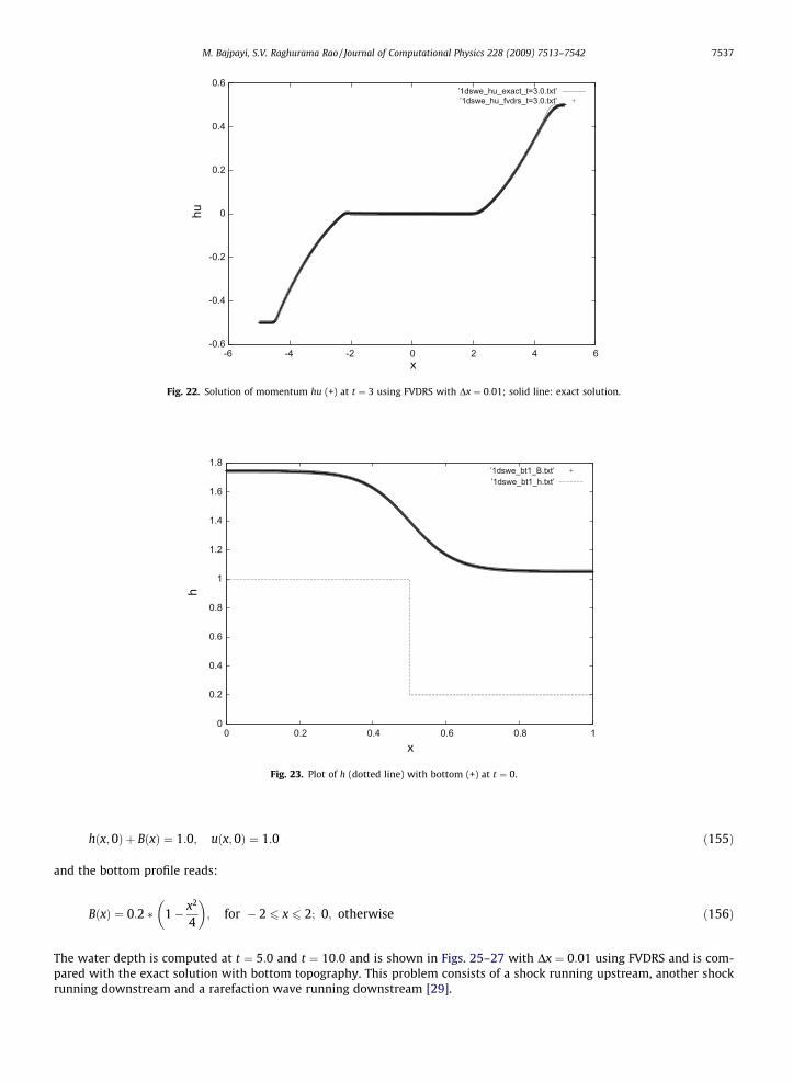
’1dswe_hu_exact_t=3.0.txt’’1dswe_hu_fvdrs_t=3.0.txt’
Fig. 22. Solution of momentum hu (+) at t ¼ 3 using FVDRS with Dx ¼ 0:01; solid line: exact solution.
0
0.2
0.4
0.6
0.8
1
1.2
1.4
1.6
1.8
0 0.2 0.4 0.6 0.8 1
h
x
’1dswe_bt1_B.txt’’1dswe_bt1_h.txt’
Fig. 23. Plot of h (dotted line) with bottom (+) at t ¼ 0.
M. Bajpayi, S.V. Raghurama Rao / Journal of Computational Physics 228 (2009) 7513–7542 7537
hðx;0Þ þ BðxÞ ¼ 1:0; uðx; 0Þ ¼ 1:0 ð155Þ
and the bottom profile reads:
BðxÞ ¼ 0:2 � 1� x2
4
� �; for � 2 6 x 6 2; 0; otherwise ð156Þ
The water depth is computed at t ¼ 5:0 and t ¼ 10:0 and is shown in Figs. 25–27 with Dx ¼ 0:01 using FVDRS and is com-pared with the exact solution with bottom topography. This problem consists of a shock running upstream, another shockrunning downstream and a rarefaction wave running downstream [29].
1
1.2
1.4
1.6
1.8
2
2.2
2.4
2.6
2.8
0 0.2 0.4 0.6 0.8 1
h+B
x
’1dswe_bt_h+B_exact_t=0.25.txt’’1dswe_bt_h+B_fvdrs_t=0.25.txt’
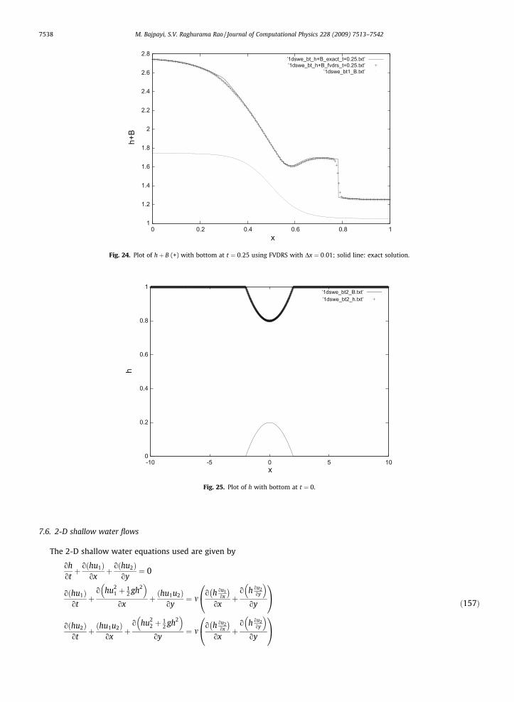
’1dswe_bt1_B.txt’
Fig. 24. Plot of hþ B (+) with bottom at t ¼ 0:25 using FVDRS with Dx ¼ 0:01; solid line: exact solution.
0
0.2
0.4
0.6
0.8
1
-10 -5 0 5 10
h
x
’1dswe_bt2_B.txt’’1dswe_bt2_h.txt’
Fig. 25. Plot of h with bottom at t ¼ 0.
7538 M. Bajpayi, S.V. Raghurama Rao / Journal of Computational Physics 228 (2009) 7513–7542
7.6. 2-D shallow water flows
The 2-D shallow water equations used are given by
ohotþ o hu1ð Þ
oxþ o hu2ð Þ
oy¼ 0
o hu1ð Þot
þo hu2
1 þ 12 gh2
�ox
þ hu1u2ð Þoy
¼ mo h ou1
ox
� ox
þo h ou2
oy
�oy
0@ 1Ao hu2ð Þ
otþ hu1u2ð Þ
oxþ
o hu22 þ 1
2 gh2 �
oy¼ m
o h ou2ox
� ox
þo h ou2
oy
�oy
0@ 1Að157Þ
0.6
0.7
0.8
0.9
1
1.1
1.2
1.3
1.4
-10 -5 0 5 10 15 20
h+B
x
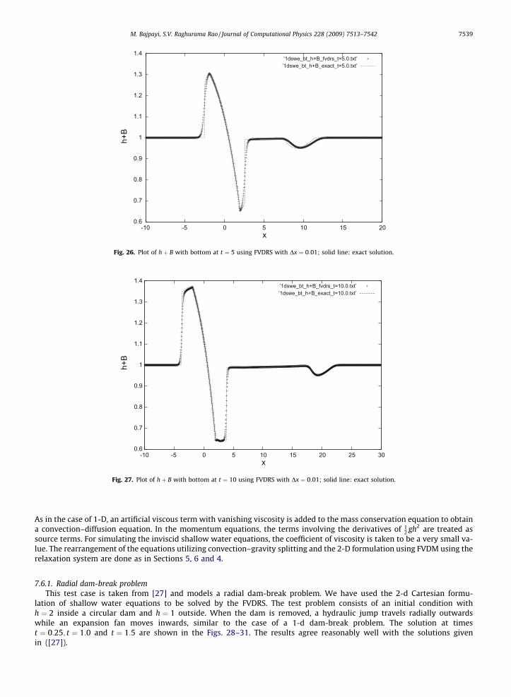
’1dswe_bt_h+B_fvdrs_t=5.0.txt’’1dswe_bt_h+B_exact_t=5.0.txt’
Fig. 26. Plot of hþ B with bottom at t ¼ 5 using FVDRS with Dx ¼ 0:01; solid line: exact solution.
0.6
0.7
0.8
0.9
1
1.1
1.2
1.3
1.4
-10 -5 0 5 10 15 20 25 30
h+B
x
’1dswe_bt_h+B_fvdrs_t=10.0.txt’’1dswe_bt_h+B_exact_t=10.0.txt’
Fig. 27. Plot of hþ B with bottom at t ¼ 10 using FVDRS with Dx ¼ 0:01; solid line: exact solution.
M. Bajpayi, S.V. Raghurama Rao / Journal of Computational Physics 228 (2009) 7513–7542 7539
As in the case of 1-D, an artificial viscous term with vanishing viscosity is added to the mass conservation equation to obtaina convection–diffusion equation. In the momentum equations, the terms involving the derivatives of 1
2 gh2 are treated assource terms. For simulating the inviscid shallow water equations, the coefficient of viscosity is taken to be a very small va-lue. The rearrangement of the equations utilizing convection–gravity splitting and the 2-D formulation using FVDM using therelaxation system are done as in Sections 5, 6 and 4.
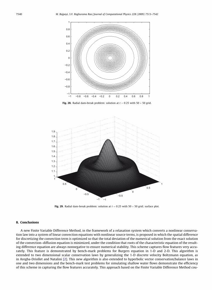
7.6.1. Radial dam-break problemThis test case is taken from [27] and models a radial dam-break problem. We have used the 2-d Cartesian formu-
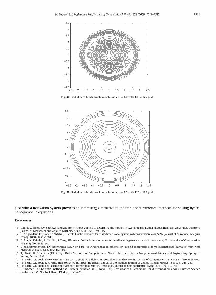
lation of shallow water equations to be solved by the FVDRS. The test problem consists of an initial condition withh ¼ 2 inside a circular dam and h ¼ 1 outside. When the dam is removed, a hydraulic jump travels radially outwardswhile an expansion fan moves inwards, similar to the case of a 1-d dam-break problem. The solution at timest ¼ 0:25; t ¼ 1:0 and t ¼ 1:5 are shown in the Figs. 28–31. The results agree reasonably well with the solutions givenin ([27]).
−1 −0.8 −0.6 −0.4 −0.2 0 0.2 0.4 0.6 0.8 1−1
−0.8
−0.6
−0.4
−0.2
0
0.2
0.4
0.6
0.8
1
Fig. 28. Radial dam-break problem: solution at t ¼ 0:25 with 50 � 50 grid.
−1−0.5
00.5
1
−1
−0.5
0
0.5
11
1.1
1.2
1.3
1.4
1.5
1.6
1.7
1.8
1.9
Fig. 29. Radial dam-break problem: solution at t ¼ 0:25 with 50 � 50 grid; surface plot.
7540 M. Bajpayi, S.V. Raghurama Rao / Journal of Computational Physics 228 (2009) 7513–7542
8. Conclusions
A new Finite Variable Difference Method, in the framework of a relaxation system which converts a nonlinear conserva-tion law into a system of linear convection equations with nonlinear source terms, is proposed in which the spatial differencefor discretizing the convection term is optimized so that the total deviation of the numerical solution from the exact solutionof the convection–diffusion equation is minimized, under the condition that roots of the characteristic equation of the result-ing difference equation are always nonnegative to ensure numerical stability. This scheme captures flow features very accu-rately. This feature is demonstrated by bench-mark problems for Burgers equation in 1-D and 2-D. This algorithm isextended to two dimensional scalar conservation laws by generalizing the 1-D discrete velocity Boltzmann equation, asin Aregba-Driollet and Natalini [2]. This new algorithm is also extended to hyperbolic vector conservation/balance laws inone and two dimensions and the bench-mark test problems for simulating shallow water flows demonstrate the efficiencyof this scheme in capturing the flow features accurately. This approach based on the Finite Variable Difference Method cou-
−2.5 −2 −1.5 −1 −0.5 0 0.5 1 1.5 2 2.5−2.5
−2
−1.5
−1
−0.5
0
0.5
1
1.5
2
2.5
Fig. 30. Radial dam-break problem: solution at t ¼ 1:0 with 125 � 125 grid.
−2.5 −2 −1.5 −1 −0.5 0 0.5 1 1.5 2 2.5−2.5
−2
−1.5
−1
−0.5
0
0.5
1
1.5
2
2.5
Fig. 31. Radial dam-break problem: solution at t ¼ 1:5 with 125 � 125 grid.
M. Bajpayi, S.V. Raghurama Rao / Journal of Computational Physics 228 (2009) 7513–7542 7541
pled with a Relaxation System provides an interesting alternative to the traditional numerical methods for solving hyper-bolic-parabolic equations.
References
[1] D.N. de G. Allen, R.V. Southwell, Relaxation methods applied to determine the motion, in two dimensions, of a viscous fluid past a cylinder, QuarterlyJournal of Mechanics and Applied Mathematics 8 (2) (1955) 129–145.
[2] D. Aregba-Driollet, Roberto Natalini, Discrete kinetic schemes for multidimensional systems of conservation laws, SIAM Journal of Numerical Analysis37 (6) (2000) 1973–2004.
[3] D. Aregba-Driollet, R. Natalini, S. Tang, Efficient diffusive kinetic schemes for nonlinear degenerate parabolic equations, Mathematics of Computation73 (245) (2004) 63–94.
[4] S. Balasubramanyam, S.V. Raghurama Rao, A grid-free upwind relaxation scheme for inviscid compressible flows, International Journal of NumericalMethods in Fluids 51 (2006) 159–196.
[5] T.J. Barth, H. Deconinck (Eds.), High-Order Methods for Computational Physics, Lecture Notes in Computational Science and Engineering, Springer-Verlag, Berlin, 1999.
[6] J.P. Boris, D.L. Book, Flux-corrected transport I: SHASTA, a fluid-transport algorithm that works, Journal of Computational Physics 11 (1973) 38–69.[7] J.P. Boris, D.L. Book, K.H. Hain, Flux-corrected transport II: generalization of the method, Journal of Computational Physics 18 (1975) 248–283.[8] J.P. Boris, D.L. Book, Flux-corrected transport III: minimal error FCT methods, Journal of Computational Physics 20 (1976) 397–431.[9] C. Fletcher, The Galerkin method and Burgers’ equation, in: J. Noye (Ed.), Computational Techniques for differential equations, Elsevier Science
Publishers B.V., North-Holland, 1984. pp. 355–475.
7542 M. Bajpayi, S.V. Raghurama Rao / Journal of Computational Physics 228 (2009) 7513–7542
[10] S.K. Godunov, A finite-difference method for the numerical computation and discontinuous solutions of the equations of fluid dynamics,Mathematicheskii Sbornik 47 (1959) 271–306.
[11] J.B. Goodman, R.J. Leveque, On the accuracy of stable schemes for 2D conservation laws, Mathematics of Computation 45 (1985) 15–21.[12] C. Günther, in: J. Noye, C. Fletcher (Eds.), Computational Techniques and Applications, Elsevier Science, Amsterdam, 1988. pp. 249–258.[13] A. Harten, The artificial compression method for computation of shocks and contact discontinuities: III. Self-adjusting hybrid schemes, Mathematics of
Computation 32 (1978) 363–369.[14] A. Harten, High-resolution schemes for hyperbolic equations and their numerical computation, Journal of Computational Physics 49 (1983) 357–393.[15] A. Harten, B. Engquist, S. Osher, S. Chakravarthy, Uniformly high-order accurate non-oscillatory schemes, Journal of Computational Physics 71 (1983)
231–303.[16] C. Hirsch, Numerical computation of internal and external flows, Fundamentals of Numerical Discretization, Vol. 1, John Wiley& Sons, 1988.[17] C. Hirsch, Numerical computation of internal and external flows, Computational Methods for Inviscid and Viscous Flows, vol. 2, John Wiley& Sons,
1990.[18] R. Holdahl, H. Holden, K.A. Lie, Unconditionally stable splitting methods for shallow water equations, BIT 39 (3) (1999) 451–472.[19] M.Y. Hussaini, B. van Leer, J. Van Rosendale (Eds.), Upwind and High-Resolution Schemes, Springer-Verlag, Berlin, 1997.[20] Shi Jin, Zhouping Xin, The relaxation schemes for systems of conservation laws in arbitrary space dimensions, Communications of Pure and Applied
Mathematics 48 (1995) 235–276.[21] S. Jin, L. Pareschi, G. Toscani, Diffusive relaxation schemes for multi-scale discrete velocity kinetic equations, SIAM Journal of Numerical Analysis 35 (6)
(1998) 2405–2439.[22] S. Jin, Efficient asymptotic-preserving (AP) schemes for some multiscale kinetic equations, SIAM Journal of Scientific Computing 21 (2) (1999) 441–
454.[23] Shi Jin, A steady-state capturing method for hyperbolic systems with geometrical source terms, Mathematical Modeling Numerical Analysis 35 (4)
(2001) 631–645.[24] Walter G. Kelley, Allan C. Peterson, Difference Equations: An Introduction with Applications, Academic Press, 2001. pp. 43–53.[25] Culbert B. Laney, Computational Gas Dynamics, Cambridge University Press, 1998.[26] R.J. Leveque, M. Pelanti, A class of approximate Riemann solvers and their relation to relaxation schemes, Journal of Computational Physics 172 (2)
(2001) 572–591.[27] R.L. Leveque, Finite Volume Methods for Hyperbolic Problems, Cambridge University Press, 2002.[28] P.L. Lions, G. Toscani, Diffusive limit for finite velocity Boltzmann kinetic models, Revista Matemtica Iberoamericana 13 (3) (1997) 473–514.[29] R. Liska, B. Wendroff, Analysis and computation with stratified fluid models, Journal of Computational Physics 137 (1997) 212–244.[30] David. K. Melgaard, Richard. F. Sincovec, General software for two dimensional non linear partial differential equations, ACM Transactions on
Mathematical Software 7 (1) (1981) 106–125.[31] Ronald E. Mickens, Non-Standard Finite Difference Models of Differential Equations, World Scientific, Singapore, 1994.[32] R. Natalini, A discrete kinetic approximation of entropy solutions to multidimensional scalar conservation laws, Journal of Differential Equations 148
(1998) 292–317.[33] J. F. Gerbeau, B. Perthame, Derivation of viscous Saint-Venant system of laminar shallow water: numerical validation, INRIA Research Report No. 4084,
2000.[34] Quirk, A contribution to the great Riemann solver debate, International Journal of Numerical Methods in Fluids 18 (1994) 555–574.[35] S.V. Raghurama Rao, New numerical schemes based on relaxation systems for conservation laws, AGTM report no. 249, Arbeitsgruppe
Technomathematik, Fachbereich Mathematik, Universitt Kaiserslautern, Germany, 2002.[36] S.V. Raghurama Rao, K. Balakrishna, An accurate shock capturing algorithm with a relaxation system for hyperbolic conservation laws, AIAA paper no.
AIAA-2003-4115, 2003.[37] S.V. Raghurama Rao, M.V Subba Rao, A simple multi-dimensional relaxation scheme for hyperbolic conservation laws, AIAA paper no. AIAA-2003-3535,
2003.[38] S.V. Raghurama Rao, Anand Tripathy, A relaxation scheme for viscous compressible flows, in: Proceedings of 6th AeSI CFD Symposium, Aeronautical
Society of India, Bangalore, August, 2003.[39] P.L. Roe, A brief introduction to high-resolution schemes, in: M.Y. Hussaini, B. van Leer, J. Van Rosendale (Eds.), Upwind and High-Resolution Schemes,
Springer-Verlag, Berlin, 1997. pp. 9–28.[40] Katsuhiro Sakai, Locally exact numerical scheme for transport equations with source terms-LENS, Journal of Nuclear Science and Technology 29 (8)
(1992) 824–827.[41] Katsuhiro Sakai, A new finite variable difference method with application to locally exact numerical scheme, Journal of Computational Physics 124
(1996) 301–308.[42] Katsuhiro Sakai, An extended finite variable difference method with application to QUICK scheme: optimized QUICK, Journal of Nuclear Science and
Technology 33 (6) (1996) 464–473.[43] Katsuhiro Sakai, A new finite variable difference method with application to nonlinear Burgers equation, Nonlinear Analysis, Theory Methods and
Applications 30 (4) (1997) 2169–2180.[44] C.W. Shu, High order ENO and WENO schemes for computational fluid dynamics, in: T.J. Barth, H. Deckoninck (Eds.), High-Order Methods for
Computational Physics, Lecture Notes in Computational Science and Engineering, Springer-Verlag, Berlin, 1999. pp. 439–582.[45] Stefan Spekreijse, Multigrid solution of monotone second-order discretizations of hyperbolic conservation laws, Mathematics of Computation 49 (179)
(1987) 135–155.[46] P.K. Sweby, High resolution schemes using flux limiters for hyperbolic conservation laws, SIAM Journal on Numerical Analysis 21 (1984) 995–1011.[47] E.F. Toro, Riemann Solvers and Numerical Methods for Fluid Dynamics, Springer, 1999.[48] Bram van Leer, Towards the ultimate conservative difference scheme II: monotonicity and conservation combined in a second-order scheme, Journal of
Computational Physics 14 (1974) 361–370.[49] Bram van Leer, Towards the ultimate conservative difference scheme III: upstream-centered finite difference schemes for ideal compressible flow,
Journal of Computational Physics 23 (1975) 263–275.[50] Bram van Leer, Towards the ultimate conservative difference scheme IV: a new approach to numerical convection, Journal of Computational Physics 23
(1975) 276–299.[51] Bram van Leer, Towards the ultimate conservative difference scheme V: a second order sequel to Godunov’s method, Journal of Computational Physics
32 (1979) 101–136.[52] Vivek Kumar, S.V. Raghurama Rao, Composite scheme using localized relaxation with non-standard finite difference method for hyperbolic
conservation laws, Journal of Sound and Vibration 311 (2008) 786–801.[53] S. Zalesak, Fully multi-dimensional flux-corrected transport algorithms for fluids, Journal of Computational Physics 31 (1979) 335–362.
Related Documents