A finite element approximation for a class of degenerate elliptic equations

MATHEMATICS OF COMPUTATIONVolume 69, Number 229, Pages 41–63S 0025-5718(99)01075-3Article electronically published on February 19, 1999

A FINITE ELEMENT APPROXIMATION FOR A CLASS OFDEGENERATE ELLIPTIC EQUATIONS

BRUNO FRANCHI AND MARIA CARLA TESI

Abstract. In this paper we exhibit a finite element method fitting a suitablegeometry naturally associated with a class of degenerate elliptic equations(usually called Grushin type equations) in a plane region, and we discuss therelated error estimates.

1. Introduction

Let Ω denote the bounded subset of R2 = Rx×Ry defined by Ω =]−1, 1[×]−1, 1[,and let Γ be its boundary. We consider the second order differential operator indivergence form in Ω defined by

L = −2∑

i,j=1

∂i(aij(z)∂j),(1.1)

where the coefficients aij = aji are measurable real-valued functions and, for someν ∈ (0, 1),

ν(ξ2 + λ2(x)η2) ≤2∑

i,j=1

aij(z)ζiζj ≤1ν

(ξ2 + λ2(x)η2)(1.2)

for any ζ = (ζ1, ζ2) = (ξ, η) and z = (x, y) ∈ R2. Here λ is a bounded nonnegativeLipschitz continuous function in R. For simplicity, the reader can think of a modeloperator of the form

L0 = −∂21 − λ2(x)∂2

2 .

Operators of this form are known as Grushin type operators, and regularity proper-ties of the weak solutions of Lu = f have been widely studied in the last few years:see, for instance, [FL], [X], [FS], [F], [FGuW1], [FGuW2]. Grushin operators canbe viewed as (generalized) Tricomi operators for transonic fluids restricted to thesubsonic region. In addition, note that every second order differential operatorin divergence form on the plane with nonnegative principal part and which is nottotally degenerate at any point (i.e. its quadratic form does not vanish identicallyat any point) can be written, after a suitable change of variables, as an operatorwhose principal part is a Grushin type operator (see [X] for an explicit calculation).

Received by the editor June 28, 1996 and, in revised form, September 8, 1997 and March 31,1998.

1991 Mathematics Subject Classification. Primary 46E30, 49N60.The first author is partially supported by M.U.R.S.T., Italy (40%) and by G.N.A.F.A. of

C.N.R., Italy (60%).The authors are indebted to A. Valli for many fruitful discussions.

c©1999 American Mathematical Society

41

License or copyright restrictions may apply to redistribution; see http://www.ams.org/journal-terms-of-use

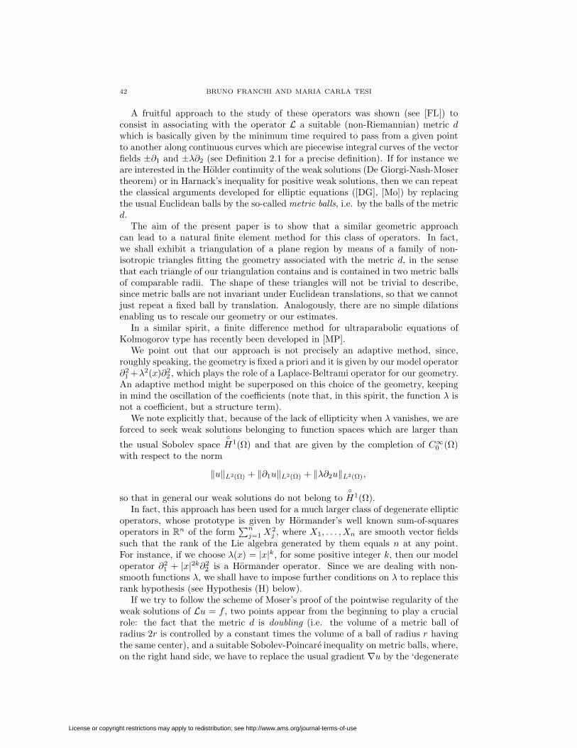
42 BRUNO FRANCHI AND MARIA CARLA TESI

A fruitful approach to the study of these operators was shown (see [FL]) toconsist in associating with the operator L a suitable (non-Riemannian) metric dwhich is basically given by the minimum time required to pass from a given pointto another along continuous curves which are piecewise integral curves of the vectorfields ±∂1 and ±λ∂2 (see Definition 2.1 for a precise definition). If for instance weare interested in the Holder continuity of the weak solutions (De Giorgi-Nash-Mosertheorem) or in Harnack’s inequality for positive weak solutions, then we can repeatthe classical arguments developed for elliptic equations ([DG], [Mo]) by replacingthe usual Euclidean balls by the so-called metric balls, i.e. by the balls of the metricd.

The aim of the present paper is to show that a similar geometric approachcan lead to a natural finite element method for this class of operators. In fact,we shall exhibit a triangulation of a plane region by means of a family of non-isotropic triangles fitting the geometry associated with the metric d, in the sensethat each triangle of our triangulation contains and is contained in two metric ballsof comparable radii. The shape of these triangles will not be trivial to describe,since metric balls are not invariant under Euclidean translations, so that we cannotjust repeat a fixed ball by translation. Analogously, there are no simple dilationsenabling us to rescale our geometry or our estimates.

In a similar spirit, a finite difference method for ultraparabolic equations ofKolmogorov type has recently been developed in [MP].

We point out that our approach is not precisely an adaptive method, since,roughly speaking, the geometry is fixed a priori and it is given by our model operator∂21 +λ2(x)∂2

2 , which plays the role of a Laplace-Beltrami operator for our geometry.An adaptive method might be superposed on this choice of the geometry, keepingin mind the oscillation of the coefficients (note that, in this spirit, the function λ isnot a coefficient, but a structure term).

We note explicitly that, because of the lack of ellipticity when λ vanishes, we areforced to seek weak solutions belonging to function spaces which are larger than

the usual Sobolev spaceH1(Ω) and that are given by the completion of C∞0 (Ω)

with respect to the norm

‖u‖L2(Ω) + ‖∂1u‖L2(Ω) + ‖λ∂2u‖L2(Ω),

so that in general our weak solutions do not belong toH1(Ω).

In fact, this approach has been used for a much larger class of degenerate ellipticoperators, whose prototype is given by Hormander’s well known sum-of-squaresoperators in Rn of the form

∑nj=1X

2j , where X1, . . . , Xn are smooth vector fields

such that the rank of the Lie algebra generated by them equals n at any point.For instance, if we choose λ(x) = |x|k, for some positive integer k, then our modeloperator ∂2

1 + |x|2k∂22 is a Hormander operator. Since we are dealing with non-

smooth functions λ, we shall have to impose further conditions on λ to replace thisrank hypothesis (see Hypothesis (H) below).

If we try to follow the scheme of Moser’s proof of the pointwise regularity of theweak solutions of Lu = f , two points appear from the beginning to play a crucialrole: the fact that the metric d is doubling (i.e. the volume of a metric ball ofradius 2r is controlled by a constant times the volume of a ball of radius r havingthe same center), and a suitable Sobolev-Poincare inequality on metric balls, where,on the right hand side, we have to replace the usual gradient ∇u by the ‘degenerate


A FINITE ELEMENT APPROXIMATION 43

gradient’ ∇λu = (∂1, λ∂2) associated with the operator. These inequalities containdeep information concerning the geometry associated with the metric d, since theyshow that the geometric dimension of the metric space defined by d is much largerthan 2 (or than n in general) and, roughly speaking, it is as large as λ is degenerate.This phenomenon has been studied in the general context of Hormander’s vectorfields, and it appears clearly in a family of isoperimetric inequalities associated witha family of such vector fields (see [FGaW], [FLW], [CDG1] [CDG2], [GN], [Gr]).

Unfortunately, this dimensional phenomenon affects our error estimates nega-tively. Indeed, first of all, we do not have any Sobolev imbedding theorem tocontrol the pointwise values of a weak solution in the interpolation operator bymeans of some higher Sobolev norm, as in the elliptic case. Roughly speaking, thisestimate is possible for a function u ∈ Hs(Rn) if n < 2s, and, as we pointed outbefore, the dimension of (Ω, d) is in general much higher than 2. Nevertheless, itis possible to bypass this difficulty, but the same dimensional phenomenon appearsagain in the numerical approximation, since, corresponding to a mesh of N points,we find in the error estimate a factor N−1/(2γ+2), where γ ≥ 0 and γ + 2 is basi-cally the geometric dimension of (Ω, d) (all these quantities will be defined formallylater). In other words, a large number of triangles is required to obtain small errors,much larger than in the elliptic case, and larger and larger as λ becomes ‘flat’ atthe points where it vanishes, so that our approximation converges, but the rate ofconvergence is affected by the order of degeneration of the function λ. Then, itis necessary to take this phenomenon into account when we compare our numeri-cal results with those we can obtain just by running numerical elliptic proceduresoutside of any theoretical scheme. Indeed, this naıve approach gives locally goodresults away from the zeros of λ (since the operator L is locally elliptic in theseregions). Note that, as we shall discuss later by means of numerical examples, ourerror estimates are sharp.

In Section 2 we characterize the geometry associated to a given class of operators,in Section 3 we set up the general framework for a finite element method fitting thegiven geometry, in Section 4 we prove error estimates and in Section 5 we discussthe algorithmic implementation of the method, and we show, by means of a suitablechoice of the right hand side of the equation, that – as we can expect – the errorestimate in the energy norm can be better than the error we obtain by using astandard mesh, or even an adaptive one (but we stress again that the use of astandard mesh has no justification, since there are solutions which do not belongto the usual Sobolev space H1(Ω)). In addition, we exhibit numerical examplesshowing that our error estimate is optimal. This will be done by analyzing theerror (in the energy norm associated with the operator) when the data have beenchosen in such a way that the solution does not belong to the usual Sobolev space.

2. Preliminaries

Through this paper we will denote a generic point in R2 by z = (x, y). In thesequel, we will assume that the function λ satisfies the following assumption:

Hypothesis (H). There exists a positive constant c1 such that, for any compactinterval I ⊆ R,

0 < c1 maxIλ ≤ 1

|I|

∫I

λ(x)dx ≤ maxIλ,

where |I| denotes the Lebesgue measure of I.



This condition is called the RH∞ condition in [F] and [FGuW1], and it impliesbasically that λ is not flat where it vanishes. For instance, if p is any polynomial inx1, then λ(x1) = |p(x1)|α (α ≥ 1) belongs to RH∞. Indeed, by rescaling, we canreduce ourselves to proving that max[0,1] |q|α ≈

∫ 1

0|q(x)|αdx when q is a polynomial

of degree ≤ m, m fixed. But both max[0,1] |q| and (∫ 1

0 |q(x)|αdx)1/α are norms onthe finite-dimensional linear space of all polynomials of degree ≤ m, and so theyare equivalent. For some comments concerning the intrinsic geometric meaning ofRH∞, see also [CF].

Let us recall now the definition of the metric associated with a family of vectorfields λ1∂1, . . . , λn∂n (see [FP], [FL], [NSW]) and the main results we will needthrough this paper.

The distance we shall define is sometimes called Carnot–Caratheodory distance,or control distance: indeed, it arises naturally in many optimal control probles (see,e.g., recent accounts in [J]).

Definition 2.1. We say that an absolutely continuous curve γ : [0, T ] → R2 is asub-unit curve if for any ζ = (ξ, η) ∈ R2,

〈γ(t), ζ〉2 ≤ |ξ|2 + λ2(γ(t))|η|2

for a.e., t ∈ [0, T ] (note that to simplify our notation we have considered λ here asa function of z ∈ R2). If z1, z2 ∈ R2, we put

d(z1, z2) = inf T > 0; there exists a sub-unit curve γ : [0, T ] → R2

such that γ(0) = z1, γ(T ) = z2.

By the assumption (H), d(z1, z2) < ∞ for any z1, z2 ∈ R2, and hence it is ametric. To prove this, we will need only to prove that we can connect each pair ofpoints z1 = (x1, y1) and z2 = (x2, y2) by means of a sub-unit curve. Arguing asin [FL] and [F], it is easy to see that we can reduce ourselves to the case x1 = x2

and λ(x1) = 0. But in that case we note that, by hypothesis (H), the functions→ λ(x1 + s) cannot vanish identically on (0, t) for any t > 0. Thus, it is enoughto move away from z1 along the segment s → (x1 + s, y1) (which is a sub-unitcurve), until we reach a point (x, y1) such that λ(x) > 0, and then we can ‘climbalong a vertical’ segment up to the point (x, y2) because s → (x, y1 + s) is also asub-unit curve. Finally, by repeating backward the previous ‘horizontal’ segmentat the level y = y2, we can achieve the proof.

Let us now introduce a function which will play a key role in the description ofthe metric balls relatives to d.

If z = (x, y) ∈ R2 and r > 0, put

F (z, r) = F (x, r) =∫ x+r

x

λ(s)ds.(2.1)

We shall see later (Theorem 2.3) that r and F (x, r) are respectively the sizes of ametric ball in the directions of the coordinate axis.

In what follows we will say that a constant c ≥ 0 is a geometric constant if itdepends on the constant c1 of Hypothesis (H) and on supλ. To avoid cumbersomenotation, at many points we will denote by the same letter c different geometricconstants.



We have:

Proposition 2.2 ([FGuW1, Proposition 2.5]). Suppose hypothesis (H) holds.Then for any point z0 = (x0, y0) ∈ R2 there exist a neighborhood U of z0 anda geometric constant γ ≥ 0 such that

(i) F (z, θt) ≥ cθ1+γF (z, t), 0 < θ < 1;(ii) F−1(z, θt) ≤ cθ1/(1+γ)F (z, t), 0 < θ < 1;(iii) F (z, θt) ≤ cθF (z, t), 0 < θ < 1;(iv) if d(z1, z2) < ct, then F (z1, t) ∼ F (z2, t),

for 0 < t < t0 and z ∈ U , where c is a geometric constant.In particular, the following crucial inequality follows from (i):∫ t

0

λ(x + sξ) ds ≥ ct1+γ(2.2)

for any z = (x, y) ∈ U , ξ ∈ S0 = ξ ∈ R : |ξ−ξ0| ≤ δ ⊂ [−1, 1]\0 and t ∈ (0, t0).

We observe that, because of Proposition 2.2 (ii), the following doubling propertyholds:

F (z, r) ≤ F (z, 2r) ≤ cF (z, r)(2.3)

for any z ∈ U , and r < r0, r0 and c being geometric constants.We can now combine Proposition 2.2 above with the characterization of the d-

balls given in [F], Theorem 2.3. The following theorem contains the description ofthe geometry given by d.

Theorem 2.3. Let the assumption (H) be satisfied. Then:(i) d(z1, z2) <∞ for any z1, z2 ∈ R2, and hence d is a metric.(ii) If we denote by B(z, r) the d-ball centered at z and of radius r (i.e. B(z, r) =

z′ ∈ R2; d(z, z′) < r), then there exist two geometric constants t1 > 0 andb > 1 such that, for any z0 ∈ R2 and t ∈ (0, t1), we have

Q(z0, t/b) ⊆ B(z0, t) ⊆ Q(z0, bt),(2.4)

where, for any r > 0,

Q(z0, r) = z = (x, y) ∈ R2 : |x− x0| < r and |y − y0| < F (z0, r).(iii) There exist two geometric constants A > 0 and r0 > 0 such that

|B(z, 2r)| ≤ A |B(z, r)|(2.5)

for any z ∈ U and r ∈ (0, r0), i.e. the metric space (R2, d) is a space ofhomogeneous type with respect to Lebesgue measure.

(iv) If θ > 0, then

c1(θ)|B(z, r)| ≤ |B(z, θr)| ≤ c2(θ)|B(z, r)|(2.6)

for any z ∈ U and r < r0 and for some suitable constants c1(θ) and c2(θ)which are geometric constants, except for the dependence on θ.

Throughout this paper, we will denote by∇λ = (∂1, λ∂2) the degenerate gradientassociated with the operator L, and we will put

|∇λu|2 = |∂1u|2 + λ2(x)|∂2u|2.(2.7)

Moreover, we will denote by H1λ(Ω) the degenerate Sobolev space associated with

∇λ, i.e. the set of u ∈ L2(Ω) such that

∂1u ∈ L2(Ω), λ∂2u ∈ L2(Ω),



endowed with the natural norm

‖u‖2H1

λ(Ω) = ‖u‖2L2(Ω) + ‖∂1u‖2

L2(Ω) + ‖λ∂2u‖2L2(Ω)(2.8)

We note that a Meyers-Serrin type theorem holds for these spaces, i.e.

C∞(Ω) ∩H1λ(Ω) is dense in H1

λ(Ω)

(see [Fr], [FSSC] and [GN]). Therefore, it will be natural to denote byH1λ(Ω) the

closure of C∞0 (Ω) in H1λ(Ω).

Hypothesis (H) implies suitable forms of classical Sobolev-Poincare inequalities,where, as we pointed out in the Introduction, the constant γ in Proposition 2.2plays the role of a dimension: see for instance [F] and [FGuW1]. However, what weneed here is only a simple form of this inequality, which states that the L2-normof a compactly supported function in Ω can be controlled by the L2-norm in Ω ofits degenerate gradients, which is therefore equivalent to the norm in H1

λ(Ω) (see,e.g., [F], Theorem 4.7).

Theorem 2.4. Suppose Hypothesis (H) holds; then there exists a geometric con-stant c > 0 such that ∫

Ω

|u|2dz ≤ c

∫Ω

|∇λu|2dz

for all u ∈H1λ(Ω).

Note that Theorem 2.4 implies that, if u ∈H1λ(Ω), then

‖u‖L2(Ω) ≤ c‖∇λu‖L2(Ω),(2.9)

so that the quadratic form

A(u, u) =∫

Ω

|∇λu|2dz

associated with the operator L is coercive onH1λ(Ω).

We can now state the main result concerning the Dirichlet problem for L in Ω.

Theorem 2.5. Let f0, f = (f1, f2) be such that f0, |f | ∈ L2(Ω). Then there exists

a unique u ∈H1λ(Ω) solution of the Dirichlet problem

(P )

Lu = −divλf + f0 in Ω,u = 0 on Γ,

(2.10)

where divλf = ∂1f1 + λ∂2f2, in the sense that

A(u, ϕ) =∫

Ω

∂1u∂1ϕ+ λ2∂2u∂2ϕdz =∫

Ω

f1∂1ϕ+ f2∂2ϕ+ f0ϕdz = Lf(ϕ)

for any ϕ ∈ C∞0 (Ω).

The proof follows straightforwardly by standard arguments from the Lax-Milgram theorem because of our Poincare inequality (Theorem 2.4).

Arguing as in [F] and in [FS], Theorems 5.11 and 6.4 respectively, we can provethe following result.

Theorem 2.6. If f0, |f | ∈ Lp for p > p0 = p0(λ), then the solution u of (P) isHolder continuous in Ω.



3. Finite element method

Let us start by constructing a triangulation of Ω which fits the geometry associ-ated with the operator. Note that the parameter n which will be considered fromnow on has nothing to do with the dimensionality of the space, which is fixed andequal to 2.

Theorem 3.1. For any n > 0 there exists a finite decomposition Tn of the domain

Ω =⋃

K∈Tn

K,

where(i) each K is a compact triangle with nonempty interior Int(K);(ii) Int(K1) ∩ Int(K2) = ∅ for distinct K1, K2 ∈ Tn;(iii) if F = K1 ∩ K2 6= ∅, where K1 and K2 are distinct elements of Tn, then

F must be a side for both K1 and K2 or a vertex for both K1 and K2 (thismeans that no vertex of one triangle lies on the edge of another triangle);

(iv) for any K ∈ Tn there exist zK , ¯zK ∈ R2 and rK , ¯rK > 0 such that

B(zK , rK) ⊆ K ⊆ B(¯zK , ¯rK), 0 < c ≤ rK¯rK

≤ C,

c and C being geometric constants;(v) supK rK ≤ const n−1/(1+γ), where γ is the constant appearing in Proposition

2.2.

Proof. Let us start by constructing the vertices of our triangulation in the set Ω+

where x ≥ 0, y ≥ 0. By reflection across the axes we will obtain all the vertices ofthe triangulation.

First, let us choose α > 0 such that α∫ 1

0 λ(s)ds = 1. Without loss of generality,we can assume that the constant c1 in Hypothesis (H) is such that αc1 < 1, and letδ0, δ1, . . . , δn be chosen so that

δ0 = 0, α

∫ δj+1

δj

λ(s)ds =1n

for j = 0, 1, . . . , n− 1.(3.1)

This choice is always possible by putting Λ(t) =∫ t0 λ(s)ds (which is strictly

increasing by Hypothesis (H)) and

δj = Λ−1( j

αn

), j = 1, . . . , n.(3.2)

Then we can consider the triangulation of Ω+

given by the family of nodes

(δj ,k

n), j = 0, . . . , n; k = 0, . . . , n.

Note that the nodes

(δn,k

n), k = 0, . . . , n,

and

(δj ,n

n), j = 0, . . . , n,

belong to Γ. From the above construction it is clear that N ∼ n2, where N is thenumber of nodes in the triangulation.



It is easy to see that the triangulation associated with this family of nodessatisfies (i)-(iii).

Let us prove (iv). To this end, let K be a triangle of Tn. Its vertices will be ofthe following forms: either

(δj ,k

n), (δj+1,

k

n), (δj+1,

k ± 1n

), j = 0, . . . , n− 1, k = 0, . . . , n− 1,

or

(δj ,k

n), (δj+1,

k

n), (δj ,

k ± 1n

), j = 0, . . . , n− 1, k = 0, . . . , n− 1.

For simplicity, let us consider only the case with K given by the vertices

P1 = (δj ,k

n), P2 = (δj+1,

k

n), P3 = (δj ,

k + 1n

).(3.3)

Set ¯zK = (δj ,k

n) and rK = max α

c1, 1 · (δj+1 − δj), where c1 is the constant of

Hypothesis (H). We have

F (¯zK , rK) =∫ δj+rK

δj

λ(s)ds ≥ c1rK max[δj ,δj+rK ]

λ

≥ α(δj+1 − δj) max[δj ,δj+1]

λ

≥ α

∫ δj+1

δj

λ(s)ds =1n

=k + 1n

− k

n,

so that:

K ⊆ Q(¯zK , rK) ⊆ B(¯zK , brK),(3.4)

and hence the second inclusion in (iv) is proved with ¯rK = brK . To prove the firstinclusion, set

zK =(δj + θ(δj+1 − δj),

k + θ

n

), rK = ε(δj+1 − δj),

where θ, ε ∈ (0, 1) are fixed constants such that θ + ε < 1/(1 + 1c1α

), ε < c1αθ.Let us prove that Q(zK , rK) ⊂ K, so that, by Theorem 2.3, we can choose

rK = rK/b. To this end, it will be enough to show that:

(a) the vertex(δj + θ(δj+1 − δj) + ε(δj+1 − δj), k+θn + F (zK , rK)

)lies below the

line z2 = 1n(δj+1−δj)−z1 + k(δj+1 − δj) + δj+1 = ψ(z1) (which connects P2

and P3),(b) the vertex

(δj + θ(δj+1 − δj)− ε(δj+1 − δj), k+θn − F (zK , rK)

)lies above the

line z2 = kn (which connects P1 and P2), and

(c) the vertex(δj + θ(δj+1− δj)− ε(δj+1− δj), k+θn −F (zK , rK)

)lies on the right

of the line z1 = δj (which connects P1 and P3).



Indeed:(a)

k + θ

n+ F (zK , rK) =

k + θ

n+

∫ δj+θ(δj+1−δj)+ε(δj+1−δj)

δj+θ(δj+1−δj)

λ(s)ds

≤ k + θ

n+ ε(δj+1 − δj) max

[δj+θ(δj+1−δj),δj+(θ+ε)(δj+1−δj)]λ

≤ k + θ

n+ ε(δj+1 − δj) max

[δj ,δj+1]λ

(since δj+1 − δj > 0 and θ + ε < 1)

≤ k + θ

n+

ε

c1

∫ δj+1

δj

λ(s)ds

(by Hypothesis (H))

=k + θ

n+

ε

αc1n<

1n

(1− θ − ε+ k)

(since 2 < 1 +1c1α

)

= ψ(δj + θ(δj+1 − δj) + ε(δj+1 − δj)

).

(b)

k + θ

n− F (zK , rK) ≥ k + θ

n− ε

αc1n

(arguing as above)

=k

n+

1n

(θ − ε

αc1) >

k

n.

(c) δj + θ(δj+1 − δj)− ε(δj+1 − δj) > δj, since ε < c1αθ < θ.To achieve the proof of (iv), we note that both rK and ¯rK are given by a geometric

constant times δj+1 − δj , so that assertion (iv) is completely proved.On the other hand, by (3.1) and (2.2),

1αn

=∫ δj+1

δj

λ(s)ds = ξ0

∫ (δj+1−δj)/ξ0

0

λ(δj + sξ0)ds ≥ c(ξ0)(δj+1 − δj)1+γ ,

and then (v) is proved.

We can proceed now in a standard way by defining a finite dimensional space Vnin the following way: Let P1, . . . , PN , N = N(n) be the nodes of Tn which belongto Int(Ω). We consider the set Φn of all continuous piecewise linear functionsϕj , j = 1, . . . , N , such that

ϕj ≡ 0 on Γ and ϕj(Pi) = δij , i = 1, . . . , N,(3.5)

and we denote by Vn the linear space generated by Φn.

Lemma 3.2. Vn ⊂H1λ(Ω) for n ≥ 1

Proof. It is enough to note that Vn ⊂H1(Ω) ⊂

H1λ(Ω).



A function vn ∈ Vn now has the representation

vn(z) =N∑i=1

vn(Pi)ϕi(z),(3.6)

and our Dirichlet problem can be approximated by the following one.Find un ∈ Vn such that

(Pn) A(un, vn) = Lf (vn) ∀vn ∈ Vn.(3.7)

As in the elliptic theory, the above problem can be solved by solving an N × Nlinear system of equations whose stiffness matrix has elements given by(

a(ϕi, ϕj))i,j=1,...,N

.

We will see in Section 5 a discussion of a numerical solution of this problem.Again as in the classical theory, we can define an interpolation operator

Πn : C0(Ω) → Vn as follows:

Πn(v) =N∑i=1

v(Pi)ϕi.(3.8)

4. Error estimate

Suppose now that f = (f1, f2) belongs to Lp(Ω) with p > p0 as in Theorem 2.6,so that the solution u of the Dirichlet problem (2.10) is continuous on Ω.

We will follow the classical Galerkin approximation scheme (see [QV], 6.2.1).This technique provides us with an error estimate giving the rate of convergenceof the approximate solutions un to u in the norm of the space of weak solutionsH1λ(Ω). It must be noticed that this error estimate is optimal, as will be clear from

the numerical results reported in Section 5. As in the usual elliptic case, the errorestimates rely on L2 estimates of the second derivatives of u; however, because ofthe lack of ellipticity when x = 0, we cannot expect usual H2 estimates to hold,but, in the spirit of our approach, if we denote by X1, X2 the vector fields ∂1 andλ(x)∂2 respectively, our second order degenerate Sobolev space H2

λ(Ω) will consistof these u ∈ H1

λ(Ω) such that each monomial XiXju belongs to L2(Ω) for i, j = 1, 2,endowed with its natural norm.

Unfortunately, the corresponding estimates up to the boundary seem rather hardto obtain. Nevertheless, if we restrict ourselves to a diagonal operator of the form

L0 = −∂21 − λ2(x)∂2

2 ,

where λ is a C0,1 function satisfying Hypothesis (H), these boundary estimates canbe deduced from analogous interior estimates.

For instance, if λ2 = µ2, where µ is a smooth function such that µ(m)(0) 6= 0for some m > 0, then these a priori interior estimates for second order ‘derivatives’hold as a particular case of a deep result of Rotschild and Stein ([RS]). Note thatif λ has such a form, then Hypothesis (H) is automatically satisfied (see below).For instance, the prototype Grushin operator corresponding to λ(x) = |x|γ satisfiesthis assumption when γ ∈ N (note that the choice of the symbol γ for the exponentis not casual here, since it is consistent with (2.2)).

Let us start with the following general result that does not rely on any particularstructure of L.



Theorem 4.1. Suppose λ is a C0,1 function satisfying Hypothesis (H) such thatλ2 ∈ C1,1, its zeros are isolated and belong to Int(Ω), and that (λ2)

′′ ≥ 0 ina neighborhood of these zeros. If f ∈ L∞(Ω), then there exists a unique u ∈H1λ(Ω) ∩C0,σ(Ω) for some σ ∈ (0, 1) such that

Lu = f in Ω.

If in addition XiXju ∈ L2(Ω) for i, j = 1, 2 (where X1 = ∂1, X2 = λ(x)∂2), then

the Galerkin approximations un ∈ Vn defined by (3.7) converge to u ∈H1λ(Ω) as

n→∞ and the following error estimate holds:

‖u− un‖H1λ(Ω) ≤ Bn−1/(1+γ),

where B depends on ‖f‖L2(Ω) and on ‖XiXju‖L2(Ω), i, j = 1, 2.

Remark. Suppose in addition we know that for any f ∈ L2(Ω) we have u ∈ H2λ(Ω)∩

H1λ(Ω). This implies that the map u→ Lu is a bijection from H2

λ(Ω)∩H1λ(Ω) onto

L2(Ω), and hence, by the closed graph theorem, the following a priori estimateholds:

2∑i,j=1

‖XiXju‖L2(Ω) ≤ C‖f‖L2(Ω).

If such an estimate holds, then the error estimate can be written in the form

‖u− un‖H1λ(Ω) ≤ Bn−1/(1+γ)‖f‖L2(Ω),

where B is a geometric constant.

Proof of Theorem 4.1. First of all we notice that f ∈⋂p≥1 L

p(Ω), and hence u ∈H1λ(Ω) ∩C0,σ(Ω) for some σ ∈ (0, 1) by Theorem 2.6.Without loss of generality, we may assume that λ(0) = 0 and λ(x) > 0 if x 6= 0.

Moreover, we can assume that λ(x′) ≥ λ(x′′) for 0 ≤ x′′ ≤ x′ and λ(x′) ≤ λ(x′′) forx′′ ≤ x′ ≤ 0. As in [QV], Theorem 5.2.1, there exist B1, B2 > 0, depending onlyon ν and the constant c of (2.9), such that

‖un‖H1λ(Ω) ≤ B1‖f‖L2(Ω),(4.1)

‖un − u‖H1λ(Ω) ≤ B2 inf

vn∈Vn

‖u− vn‖H1λ(Ω).(4.2)

On the other hand,

infvn∈Vn

‖u− vn‖H1λ(Ω) ≤ ‖u−Πn(u)‖H1

λ(Ω),(4.3)

since Πn(u) is well defined because of the continuity of u and it belongs to Vnbecause of Lemma 3.2. By combining (4.2) and (4.3) it will follow that un → u inH1λ(Ω) once we have proved that ‖u−Πn(u)‖H1

λ(Ω) → 0 as n→∞.Now

‖u−Πn(u)‖H1λ(Ω) ≤ c

‖u−Πn(u)‖L2(Ω) + ‖∇λ(u −Πn(u))‖L2(Ω)

= c

∑K∈Tn

‖u−Πn(u)‖L2(K) + ‖∇λ(u−Πn(u))‖L2(K)

.(4.4)



We have:

Lemma 4.2. There exists a geometric constant B3 > 0 such that, if we put X1 =∂1, X2 = λ∂2, then, if K ∈ Tn,

‖u−Πn(u)‖L2(K) + ‖∇λ(u −Πn(u))‖L2(K)

≤ B3

‖X2

1u‖L2(K) + ‖X22u‖L2(K) + ‖X2X1u‖L2(K)

n−1/(1+γ).(4.5)

Note that Int(K) intersects neither Γ nor the degeneration line x = 0, so thatu ∈ C2,α

loc (IntK), by classical Schauder estimates.

Proof. First, let us estimate∫K

|∇λ(u−Πn(u))|2dxdy =∫K

|∇λ(u−3∑i=1

u(Qi)ϕi)|2dxdy = I2,(4.6)

where Q1, Q2, Q3 are the vertices of K.Suppose for instance that K has vertices (δj , kn ), (δj+1,

kn ), (δj , k+1

n ), and putx = δj + (δj+1 − δj)x′,y = k

n + 1ny

′ .(4.7)

The above change of variables maps K onto the base triangle of vertices (0,0), (1,0),(0,1), and its Jacobian determinant is 2|K|, so that, if we denote by v any functionv written in the new variables x′, y′, we get∫

K

|v −Πn(v)|2dxdy = 2|K|∫K

|v −3∑i=1

v(Qi)ϕi|2dx′dy′(4.8)

Note now that∂x′ v = (δj+1 − δj)∂xv, ∂y′ v =

1n∂yv.

Then∫K

|∂x(u−3∑i=1

u(Qi)ϕi)|2dxdy = 2|K|∫K

|∂x(...)|2dx′dy′

=2|K|

(δj+1 − δj)2

∫K

|∂x′ (...)|2dx′dy′

=1

n(δj+1 − δj)

∫K

|∂x′ (...)|2dx′dy′.(4.9)

Analogously∫K

|λ(x)∂y(u−3∑i=1

u(Qi)ϕi)|2dxdy

= n(δj+1 − δj)∫K

λ2(δj + (δj+1 − δj)x′)|∂y′ (...)|2dx′dy′

≤ n(δj+1 − δj) · ( max[δj ,δj+1]

λ)2∫K

|∂y′ (...)|2dx′dy′

≤ 1c12

n

(δj+1 − δj)

(∫ δj+1

δj

λ(t)dt)2

∫K

|∂y′ (...)|2dx′dy′

= c1

n(δj+1 − δj)

∫K

|∂y′ (...)|2dx′dy′, by (3.1),



so that

I2 ≤ c1

n(δj+1 − δj)|u−

3∑i=1

u(Qi)ϕi|2H1(K),(4.10)

where Q1, Q2, Q3 are vertices of K, and | · |Hk(K) denotes the seminorm given by thesum of the L2−norms of the highest derivatives. We can now apply the followingclassical estimate:

|u−3∑i=1

u(Qi)ϕi|2H1(K)≤ c|u|2

H2(K)(4.11)

(see, for instance [QV], Theorem 3.4.1), and we get

I2 ≤ c1

n(δj+1 − δj)

‖∂2x′ u‖2

L2(K)+ ‖∂2

y′ u‖2L2(K)

+ ‖∂y′∂x′ u‖2L2(K)

= c

(δj+1 − δj)3

n‖∂2xu‖2

L2(K)+

1n5(δj+1 − δj)

‖∂2yu‖2

L2(K)

+(δj+1 − δj)

n3‖∂y∂xu‖2

L2(K)

= c

(δj+1 − δj)2‖∂2

xu‖2L2(K) +

1n4‖∂2yu‖2

L2(K) +1n2‖∂y∂xu‖2

L2(K)

= J1 + J2 + J3.

(4.12)

First of all, we note that J1 can be written as follows:

J1 = (δj+1 − δj)2‖X21u‖2

L2(K);

the next step will consist of proving that

J2 ≤ c(δj+1 − δj)2‖X22u‖2

L2(K) and J3 ≤ c(δj+1 − δj)2‖X2X1u‖2L2(K).(4.13)

To this end, we observe that, if x ∈ K, then, by the monotonicity of λ,

λ(x) ≥ λ(δj) ≥1

δj − δj−1

∫ δj

δj−1

λ(t)dt =1

n(δj − δj−1),

so that (4.13) will follow by proving that

δj − δj−1 ≤ c(δj+1 − δj)(4.14)

for all j = 0, 1, . . . , n− 1.On the other hand, it is easy to see that

d((δj−1, k/n), (δj , k/n)) ≤ δj − δj−1,

so that, by Proposition 2.2 (iv), we have

F ((δj , k/n),δj − δj−1) ≤ cF ((δj−1, k/n), δj − δj−1)

= c

∫ δj

δj−1

λ(t)dt =c

αn= c

∫ δj+1

δj

λ(t)dt

= cF ((δj , k/n), δj+1 − δj) ≤ F ((δj , k/n), c′(δj+1 − δj)),

by Proposition 2.2 (iii), and hence (4.14) follows by the monotonicity of the functiont→ F ((δj , k/n), t).



Thus

I2 ≤ c(δj+1 − δj)2‖X2

1u‖2L2(K) + ‖X2

2u‖2L2(K) + ‖X2X1u‖2

L2(K)

≤ n−2/(1+γ)

‖X2

1u‖2L2(K) + ‖X2

2u‖2L2(K) + ‖X2X1u‖2

L2(K)

,

by Theorem 3.1 (iv) and (v). Finally, the term

I1 =∫K

|u− Πn(u)|2dxdy

can be handled in the same way.Combining (4.4) and (4.5), we complete the proof of Theorem 4.1.

Theorem 4.3. Let λ be as in Theorem 4.1, and let the following interior a prioriestimate hold: if v ∈ H1

λ,loc(R2) is such that L0v = g ∈ L2(Ω), then for anyψ ∈ C∞0 (R2) ∑

i,j=1,2

‖XiXj(ψv)‖L2(Ω) ≤ Cψ‖g‖L2(Ω).

Then the following error estimate for the Galerkin approximations of the solution

u ∈H1λ(Ω) of L0u = f ∈ L∞(Ω) holds:

‖u− un‖H1λ(Ω) ≤ Bn−1/(1+γ)‖f‖L2(Ω),

where B is a geometric constant.

Proof. By Theorem 4.1 and the subsequent remark, we have only to prove thatXiXju ∈ L2(Ω) for i, j = 1, 2. Consider the following covering Fj for Ω:F1 =] − ∞,−1/4[×R, F2 =]1/4,+∞[×R, F3 =] − 1/3, 1/3[×]− 3/4, 3/4[, F4 = e2+]−1/3, 1/3[×]−1/3, 1/3[, F5 = −e2+]−1/3, 1/3[×]−1/3, 1/3[, where e2 = (0, 1).Let moreover ψj, j = 1, 2, 3, 4, 5 be a partition of unity subordinate to the cover-ing Fj, with ψj ∈ C∞

0 (R2), 0 ≤ ψj ≤ 1, supp ψj ⊂ Fj . We have∑i,j

‖XiXju‖L2(Ω) ≤∑k

∑i,j

‖XiXj(ψku)‖L2(Fk).

Consider now k = 1, 2: these cases can be easily reduced to usual elliptic estimates.Indeed, in F1 and F2 the H2

λ norm is equivalent to the usual Sobolev norm, forλ is bounded away from zero on these regions. On the other hand, for the samereason, the operator L0 is elliptic on F1 and F2, and then it satisfies standard H2

a priori estimates by a well known regularity result on planar angular regions dueto P. Grisvard ([G]). Thus, if we take into account that

L0(ψku) = ψkf − 2〈∇λψk,∇λu〉 − uL0ψk = gk,

and that ‖gk‖L2(Ω) ≤ c‖f‖L2(Ω), we get for k = 1, 2∑i,j

‖XiXj(ψku)‖L2(Fk) ≤ c‖ψku‖H2(Ω) ≤ c‖L0(ψku)‖L2(Ω) + ‖ψku‖L2(Ω)

≤ c‖f‖L2(Ω).

Thus we can restrict ourselves to considering, for instance, the region F4. We setF4 = Q, Q− = e2+]− 1/3, 1/3[×]− 1/3, 0[ and Q+ = e2+]− 1/3, 1/3[×]0, 1/3[. Wecan assume that ψ4 = ψ satisfies ψ ≡ 1 on B(e2, 1/4).



As above, uψ ∈H1λ(Ω) and L0(uψ) = g ∈ L2(Ω), with ‖g‖L2(Ω) ≤ c‖f‖L2(Ω).

We now define

G1(x, y) =

g in Q−,

0 in Q+,

and we denote by v1 ∈H1λ(Q) the solution of the problem

(P1)

L0v1 = G1 in Q,

v1 = 0 on ∂Q.

Let G2(x, y) = G1(x, 2 − y) and let v2 ∈H1λ(Q) be the solution of the problem

(P2)

L0v2 = G2 in Q,

v2 = 0 on ∂Q.

We have:(1) v1, v2 ∈ C0,α(Q);(2) v2(x, y) = v1(x, 2− y).

The first property holds as above, arguing as in [FS], whereas the second propertyfollows from the uniqueness of the solution of (P2), if we prove that v1(x, 2 − y)solves (P2). To this end, let ϕ ∈ C∞0 (Q); then∫

Q

[(v1)x(x, 2− y)ϕx(x, y)− λ2(x)(v1)2−y(x, 2 − y)ϕy (x, y)] dxdy

=∫Q

[(v1)x(x, η)ϕx(x, 2− η)− λ2(x)(v1)η(x, η)ϕ2−η(x, 2 − η)

]dxdη

=∫Q

[(v1)x(x, η)ψx(x, η) + λ2(x)(v1)η(x, η)ψη(x, η)

]dxdη

(where ψ(x, η) = ϕ(x, 2 − η))

=∫Q

G1(x, η)ψ(x, η)dxdη =∫Q

G1(x, η)ϕ(x, 2 − η)dxdη

=∫Q

G1(x, 2 − y)ϕ(x, y)dxdy

=∫Q

G2(x, y)ϕ(x, y)dxdy.

Now we put v = (v1 − v2)∣∣Q−

, so that v(x, y) = (v1(x, y)− v1(x, 2 − y))∣∣Q−, v ∈

C0,α(Q−) and v ≡ 0 on ∂Q−. Moreover, v ∈ H1λ(Q−). We assume we have proved

that v ∈H1λ(Q−), and we verify that L0v = g in Q−. Let ϕ ∈ C∞0 (Q−); then∫

Q−(vxϕx + λ2vyϕy)dxdy

=∫Q−

[(v1)xϕx + λ2(v1)yϕy

]dxdy −

∫Q−

[(v2)xϕx + λ2(v2)yϕy

]dxdy

=∫Q−

(G1 −G2)ϕdxdy =∫Q−

gϕdxdy,

since G1 ≡ g in Q− and G2 ≡ 0 in Q−. Hence by uniqueness v = uψ.



We prove now that if v ∈ H1λ(Q−) ∩ C0,α(Q−) and v ≡ 0 on ∂Q−, then

v ∈H1λ(Q−). To this end we consider the covering for Q− given by E1 = Q− ∩

(]−∞,−1/4[×R), E2 = Q− ∩ (]1/4,+∞[×R), E3 = Q− ∩ (R×]1 − 2δ,+∞[), E4 =Q− ∩ (R×]1 − δ,−∞[), and let ϕi, i = 1, 2, 3, 4, be a partition of unity sub-

ordinate to this covering. It will be enough to prove that vϕi ∈H1λ(Q−) for

i = 1, 2, 3, 4. This is clear for vϕ1 and vϕ2, since vϕ1, vϕ2 ∈ H1(Q−) and so

v ∈H1(Q−) ⊆

H1λ(Q−) by the usual results on Sobolev spaces. We now prove that

vϕ3 = v ∈H1λ(Q−); vϕ4 can be treated analogously. To prove that v ∈

H1λ(Q−)

we will prove that v can be approximated by functions vn ∈ H1λ(Q−) such that

supp vn ⊂ Q−. Indeed, since the usual convolutions with Friedrich’s mollifiers doconverge in H1

λ(Q−) ([FSSC], [GN]), each vn can be approximated in H1λ(Q−) by

functions in C∞0 (Q−), and hence the statement follows.Let ψn : [0,+∞) → [0 : +∞) be a smooth function such that ψn ≡ 1 on

[0, 1 − 1/n], ψn ≡ 0 on [1 − 1/2n,+∞), 0 ≤ ψn ≤ 1, |ψ′n| ≤ 3n: we set vn = ψnv.

It follows that supp vn ⊂ Q− and ‖vn − v‖L2(Q−) = ‖v(ψn − 1)‖L2(Q−). Nowv(ψn − 1) → 0 a.e. and |v(ψn − 1)| ≤ |v|, and hence the norm tends to zero.Therefore vn → v in L2(Q−). Analogously ∂xvn → ∂xv in L2(Q−). Assume wehave proved that ‖λ∂y vn‖L2(Q−) ≤ C. It follows from the reflexivity of H1

λ(Q−)that (vn)n∈N converges weakly in H1

λ(Q−), and then vn → v weakly in H1λ(Q−)

since v ∈ H1λ(Q−) and vn → v in L2(Q−). Hence, by Mazur’s theorem, v is the

limit in H1λ(Q−) of a sequence of finite convex combinations of vk, k ∈ N which

are still functions supported in Q−, and we are done.Let us prove now that ‖λ∂y vn‖L2(Q−) is bounded. We notice that

∂v

∂y∈ L2(Q− ∩ |x| ≥ ε)

for every ε > 0, and hence the function y → ∂v∂y (x, y) is in L1

loc for almost every x.Therefore, using the property v(x, 1) ≡ 0, we have

|v(x, y)| ≤∫ 1

y

|∂v∂y

(x, t)|dt ≤√

1− y

(∫ 1

y

|∂v∂y|2dt

)1/2

for (x, y) ∈ Q−. We then have

‖λ∂y vn‖L2(Q−) ≤ ‖λψn(∂y v)‖L2(Q−) + ‖λv(∂yψn)‖L2(Q−).

The first term tends to ‖λ∂y v‖L2(Q−) as n→∞, as above. Concerning the secondone, we have

‖λv(∂yψn)‖2L2(Q−) ≤ 9n2

∫ 1/3

−1/3

dxλ2(x)∫ 1

1−1/n

dyv2(x, y)

≤ 9n2

∫ 1/3

−1/3

dxλ2(x)∫ 1

1−1/n

dy(1− y)∫ 1

2/3

|∂v∂y

(x, t)|2dt

= 9n2

∫Q−

dxdt|λ∂v∂y

(x, t)|2∫ 1

1−1/n

dy(1− y)

=92‖λ∂v∂y‖2L2(Q−),

and the statement is proved.



Now results on interior regularity for problems (P1) and (P2) guarantee thatX2

1vi, X1X2vi, X2X1vi, X22vi ∈ L2(B(e2, 1/4)), and hence it follows that X2

1u,X1X2u, X2X1u,X

22u ∈ L2(Ω).

Corollary 4.4. Let λ be such that λ = |µ|, where µ is a smooth function such that

µ(0) = µ′(0) = · · · = µ(m−1)(0) = 0

and µ(m)(0) 6= 0 for some m ≥ 1. Then the conclusion of Theorem 4.3 holds.

Proof. The two vector fields Y1 = ∂1, Y2 = µ∂2 satisfy Hormander’s rank conditionsince the rank of the Lie algebra generated by Y1 and Y2 equals 2 at each point ofR2. Thus the interior a priori estimate of Theorem 4.3 follows from Theorem 16(d) in [RS]. Thus we have only to show that Hypothesis (H) is satisfied, since theremaining assumptions of Theorem 4.1 follow straightforwardly. On the other hand,Hypothesis (H) follows by Proposition 5 in [FW], where it is shown in particularthat, because of the Hormander condition, the function µ belongs to RH∞, i.e. itsaverage on any interval is equivalent to its L1 norm on the same interval, and sowe are done.

5. Algorithm and numerical results

In this section we will describe some numerical tests of our previous results; aswe pointed out in the Introduction, the number γ+2 plays the role of a dimension,which can be very large if the operator is strongly degenerate. Because of this, totest the trend of our estimates we have to work with a mesh containing a largenumber of points, and, for this reason, we have to choose our implementationrather carefully. The algorithm we used to perform our numerical integrations isMGGHAT, a unified multilevel adaptive refinement method, in which a unifiedapproach to the combined processes of adaptive refinement and multigrid solutionhas been very conveniently implemented. A detailed technical description of themethod can be found in [M1], [M2].

In our case the refinement cannot be obviously performed by bisecting pairs oftriangles, since we want to reproduce the geometry associated with the differentialoperator considered. The hierarchical basis scheme can nevertheless be applied,since also for the geometries considered in this paper it is possible to implementdivisions (which reproduce the geometry required) of a pair of triangles, correspond-ing to the addition of a new basis function having support for the pair of trianglesdivided, and leaving the existing basis functions unchanged; in fact we modified thepart of the program producing the mesh generation, according to our geometry.

Indeed, from (3.2) it can be seen that at each level of refinement all the oldnodes are maintained, and some new ones are added. This is exactly the principleon which the hierarchical basis approach is based. The hierarchical basis coincideswith the usual nodal basis at the first level of refinement. As refinement proceeds,with each division one or more new nodes are added, and for each node a newbasis function is defined so that it has the value 1 at the new node and 0 at allother nodes, but the existing basis functions remain unchanged. The choice ofhierarchical basis leads to a representation of Πn(u) which differs from (3.8), andthen to a different stiffness matrix: the algorithmical gain is described in [BDY]and [M2].



As an example, we choose

λ =√βm|x|m−1 for β > 0 and m > 1,

so that it is easy to check that (2.2) holds with γ = m− 1. Put

R = β|x|2m + y2 and u = R1/m,

and, finally,

v = (1 − x2)(1 − y2)u.

A direct calculation shows that v ∈H1λ(Ω), and that f = L0v ∈ L∞(Ω); on the

other hand, if m > 2.5, then v does not belong to the usual Sobolev spaceH1(Ω).

This fact is not surprising, since the function u is equivalent to the square of thedistance d of the point (x, y) from the origin (see [FL]), so that it reflects in a rathersubtle way the properties of the model operator L0 and it is strictly connected with

the Sobolev spaceH1λ(Ω).

We can now evaluate the discretization error in the energy norm

‖∂x(v − vn)‖L2(Ω) + ‖λ∂y(v − vn)‖L2(Ω),

which not only is the norm naturally associated with the operator, but it also is theonly ‘reasonable’ norm, since in general the H1-norm of v is infinite. By Theorem

2.4, the energy norm is equivalent to the norm inH1λ(Ω).

In the following pictures we plotted these errors in a log-log scale as a functionof N , the number of the nodes of our triangulation, which we recall is proportionalto n2 (we call the triangulation corresponding to the geometry naturally associatedto the operator the natural triangulation, see Figure 3), and we compared it withthe errors we obtain (for the same number of nodes) by using an adaptive version ofour triangulation, a uniform triangulation and an adaptive uniform triangulation.The graphs in Figure 1 correspond to β = 128 and m = 4 (γ = 3) and m = 6(γ = 5), respectively. The choice of a large β has been suggested by the need ofamplifying the behaviors we are interested in studying.

Finally, we evaluated the trend of the error estimate, reported in Table 1, bycomparing it with the theoretical estimate (always in the same logarithmic scale)in the cases m = 2 (γ = 1) and m = 3 (γ = 2). The expected trend for theerrors is of the form N b, where by our error estimate b = −0.25 for γ = 1 andb = −0.16 for γ = 2. The results obtained from the linear fitting of the data, i.e.b = −0.242± 0.008 for γ = 1 and b = −0.17± 0.01 for γ = 2, shown in Figure 2,are a clear indication of the optimality of the error estimate.



Figure 1. Plot of the discretization error in energy norm, as afunction of the number of nodes N , obtained with four differenttriangulation types: natural (i.e. obtained using the geometry nat-urally associated to the operator), uniform (i.e. obtained usingEuclidean geometry), adaptive uniform (i.e. obtained by an adap-tive refinement method in the Euclidean geometry) and adaptivenatural (i.e. obtained by an adaptive refinement method in thegeometry naturally associated to the operator); for γ = 3 (m = 4)(Figure 1a, top) and γ = 5 (m = 6) (Figure 1b, bottom).



Figure 2. Fitting of the discretization error in H1λ norm for

γ = 1 (m = 2) (Figure 2a, top) and γ = 2 (m = 3) (Figure2b, bottom). The smaller nodes have been discarded to consideronly the asymptotic regime. The line superimposed on the data isthe result of numerical fit. The data have been fitted with the lin-ear function f(N) = a×N b, where N is the number of nodes usedin the triangulation. We obtained the values b = −0.242 ± 0.008for γ = 1, corresponding to the theoretical prediction b = −0.25,and b = −0.17 ± 0.01 for γ = 2, corresponding to the theoreticalprediction b = −0.16. The set of data used are also reported inTable 1.



Table 1

N γ = 1 γ = 2545 0.14831089 0.12792113 0.1039 0.12654225 0.0895 0.10808321 0.0763 0.097816641 0.0674 0.0877

Figure 3. Example of a triangulation with 128 triangles obtainedwith the geometry naturally associate to the operator, with γ =1 (m = 2).

References

[BDY] R.E. Bank, T.F. Dupont and H. Yserentant, The hierarchical basis multigrid method,Num. Math. 52 (1988), 427–458. MR 89b:65247

[CDG1] L. Capogna, D. Danielli and N. Garofalo, The geometric Sobolev embedding for vectorfields and the isoperimetric inequality, Comm. in Analysis and Geometry 2 (1994),203–215. MR 96d:46032

[CDG2] , Subelliptic mollifiers and a basic pointwise estimate of Poincare type, Math.Z. 226 (1997), 147–154. MR 98i:35025

[CF] C. Cancelier and B. Franchi, Subelliptic estimates for a class of degenerate ellipticintegro–differential operators, Math. Nachr. 183 (1997), 19–41. MR 98d:35086

[DG] E. De Giorgi, Sulla differenziabilita e l’analiticita degli integrali multipli regolari, Mem.Accad. Sci. Torino Cl. Sci. Fis. Mat. Natur. 3 (1957), 25–43. MR 20:172



[F] B. Franchi, Weighted Sobolev-Poincare inequalities and pointwise estimates for a classof degenerate elliptic equations, Trans. Amer. Math. Soc. 327 (1991), 125–158. MR91m:35095

[Fr] K.O. Friedrichs, The identity of weak and strong estension of differential operators,Trans. Amer. Math. Soc. 55 (1944), 132–151. MR 5:188b

[FGaW] B. Franchi, S. Gallot and R.L. Wheeden, Sobolev and isoperimetric inequalities fordegenerate metrics, Math. Ann. 300 (1994), 557–571. MR 96a:46066

[FGuW1] B. Franchi, C. Gutierrez and R.L. Wheeden, Weighted Sobolev-Poincare inequalitiesfor Grushin type operators, Comm. Partial Differential Equations 19 (1994), 523–604.MR 96h:26019

[FGuW2] B. Franchi, C. Gutierrez and R.L. Wheeden, Two-weight Sobolev-Poincare inequalitiesand Harnak inequality for a class of degenerate elliptic operators, Atti Accad. Naz.Lincei, Cl. Sci. Fis. Mat. Natur 5 (9) (1994), 167–175. MR 95i:35115

[FL] B. Franchi and E. Lanconelli, Holder regularity theorem for a class of linear nonuni-

formly elliptic operators with measurable coefficients, Ann. Scuola Norm. Sup. Pisa 10(4) (1983), 523–541. MR 85k:35094

[FLW] B. Franchi, G. Lu and R.L. Wheeden, Representation formulas and weighted Poincareinequalities for Hormander vector fields, Ann. Inst. Fourier, Grenoble 45 (1995), 577–604. MR 96i:46037

[FP] C. Fefferman and D.H. Phong, Subelliptic eigenvalue problems, Conference on HarmonicAnalysis, Chicago, 1980, (W. Beckner et al., eds.), Wadsworth, 1981, pp. 590–606. MR86c:35112

[FS] B. Franchi and R. Serapioni, Pointwise estimates for a class of strongly degenerateelliptic operators: a geometrical approach, Ann. Scuola Norm. Sup. Pisa 14 (4) (1987),527–568. MR 90e:35076

[FSSC] B. Franchi, R. Serapioni and F. Serra Cassano, Champs de vecteurs, theoreme d’appro-ximation de Meyers-Serrin et phenomeme de Lavrentev pour des fonctionnelles dege-neres, C.R. Acad. Sci. Paris Ser. I Math. 320 (1995), 695–698. MR 95m:46044

[FW] B. Franchi and R.L. Wheeden, Compensation couples and isoperimetric estimates forvector fields, Colloq. Math 74 (1997), 9–27. MR 98g:46042

[G] P. Grisvard, Behaviour of the solutions of an elliptic boundary value problem in apolygonal or polyhedral domain, Numerical Solutions of Partial Differential Equations,III (B. Hubbard, ed.), Academic Press, New York, 1976, pp. 207–274. MR 57:6786

[Gr] M. Gromov, Carnot-Caratheodory spaces seen from within, Sub–Riemannian Geometry,Birkhauser, 1996, pp. 79–323. CMP 97:04

[GN] N. Garofalo and D.M. Nhieu, Isoperimetric and Sobolev inequalities for Carnot-Cara-theodory spaces and the existence of minimal surfaces, Comm. Pure Appl. Math. 49(1996), 1081–1144. MR 97i:58032

[GT] D. Gilbarg and N.S. Trudinger, Elliptic Partial Differential Equations of Second Order,Springer, Berlin, 1977. MR 57:13109

[J] V. Jurdjevic, Geometric Control Theory, Cambridge Studies in Advanced Mathematics,1997. MR 98a:93002

[Mo] J. Moser, A new proof of De Giorgi’s theorem concerning the regularity problem forelliptic differential equations, Comm. Pure Appl. Math. 13 (1961), 457–468. MR 30:332

[M1] W.F. Mitchell, Unified multilevel adaptive finite element method for elliptic problems,Ph.D. thesis, Report No. UIUCDSC-R-88-1436, Department of Computer Science, Uni-versity of Illinois, Urbana, IL, 1988.

[M2] W.F. Mitchell, Optimal multilevel iterative methods for adaptive grids, SIAM J. Sci.Stat. Comput. 13 (1992), 146–167. MR 92j:65187

[MP] C. Mogavero and S. Polidoro, A finite difference method for a boundary value problemrelated to the Kolmogorov equation, Calcolo 32 (1995), 193–206. CMP 98:04

[NSW] A. Nagel, E.M. Stein and S. Wainger, Balls and metrics defined by vector fields I: basicproperties, Acta Math. 155 (1985), 103–147. MR 86k:46049

[QV] A. Quarteroni and A. Valli, Numerical Approximation of Partial Differential Equations,Springer Series in Computational Mathematics, Springer, Berlin, 1994. MR 95i:65006

[RS] L.P. Rothschild and E.M.Stein, Hypoelliptic differential operators and nilpotent groups,Acta Math. 137 (1976), 247-320. MR 55:9171



[X] C.-J. Xu, The Harnack’s inequality for second order degenerate elliptic operators, Chi-nese Ann. Math. Ser A 10 (1989), 359–365, in Chinese. MR 90m:35039

Dipartimento Matematico dell’Universita, Piazza di Porta S. Donato, 5, 40127 Bolo-

gna, Italy

E-mail address: [email protected]

Universite de Paris-Sud, Mathematiques, Bat. 425, 91405 Orsay Cedex, France

E-mail address: [email protected]


A finite element approximation for a class of degenerate elliptic equations

Documents