A feedback approach to the steady-state performance of fractionally spaced blind adaptive equalizers

$Page 1: A feedback approach to the steady-state performance of fractionally spaced blind adaptive equalizers$
80 IEEE TRANSACTIONS ON SIGNAL PROCESSING, VOL. 48, NO. 1, JANUARY 2000

A Feedback Approach to the Steady-StatePerformance of Fractionally Spaced Blind Adaptive

EqualizersJunyu Mai and Ali H. Sayed, Senior Member, IEEE

Abstract—This paper proposes a new approach to the analysisof the steady-state performance of constant modulus algorithms(CMA), which are among the most popular adaptive schemesfor blind equalization. A major feature of the proposed feedbackapproach is that it bypasses the need for working directly withthe weight error covariance matrix. In so doing, approximateexpressions for the steady-state mean-square error of several CMalgorithms are derived, including CMA2-2, CMA1-2, normalizedCMA, and a new normalized CMA variant with less bias. Acomparison among the various algorithms is also performed,along with several simulation results. The conclusions confirm thesuperior performance of CMA2-2.

Index Terms—Adaptive filter, blind equalization, constant mod-ulus signal, feedback analysis, mean-square error.

I. INTRODUCTION

A MONG the most popular adaptive schemes for blindequalization are the so-called constant modulus algo-

rithms (CMA’s); see [1]–[3] and the many references therein.The update equations of these algorithms are nonlinear innature, which may explain why only a handful of resultsare available in the literature regarding their steady-statemean-square-error performance. The difficulty arises from thefact that classical approaches to steady-state performance eval-uation often require, as an intermediate step, that a recursionbe determined for the covariance matrix of the weight errorvector. This step can become a burden for CM algorithms dueto their inherent nonlinear updates (see, e.g., the analysis of theconstant modulus array algorithm for adaptive beamforming in[4] and the analysis of the performance of CMA for interferencecancellation in [5, Sec. 3.3]).

The main objective of this paper is to propose a new approachto the analysis of the steady-state performance of blind adap-tive algorithms. A major feature of the approach is that it by-passes the need to work directly with the weight error vector.In so doing, approximate expressions for the steady-state mean-square error of several CM algorithms are derived (including

Manuscript received November 20, 1998; revised June 20 1999. This workwas supported in part by the National Science Foundation under Awards MIP-9796147 and CCR-9732376. The associate editor coordinating the review ofthis paper and approving it for publication was Dr. Xiang-Gen Xia.

J. Mai was with the Electrical Engineering Department, University of Cali-fornia, Los Angeles, CA 90024 USA. She is now with the Advanced ResearchDepartment, St. Jude Medical Cardiac Rhythm Management Division, Sylmar,CA 91342 USA.

A. H. Sayed is with the Electrical Engineering Department, University ofCalifornia, Los Angeles, CA 90024 USA (e-mail: [email protected]).

Publisher Item Identifier S 1053-587X(00)00099-4.

CMA2-2, CMA1-2, normalized CMA, and a new normalizedCMA variant with less bias). A comparison among the variousalgorithms is also performed, along with several simulation re-sults. Our conclusions will further confirm the superior perfor-mance of CMA2-2.

The approach in this paper exploits a fundamental energy-preserving relation that, in fact, holds for a general class of adap-tive filters and not just CM algorithms [6]. This relation allowsus to avoid working directly with the nonlinear update that ischaracteristic of CM algorithms; it focuses instead on the prop-agation of error energies through a feedback structure that con-sists of a lossless feedforward block and a feedback path.

A. Earlier Results in the Literature

Some of the earlier results in the literature on the performanceof CM algorithms that are relevant to the discussion in this paperappear in [9]–[13]. The survey article [3] provides a compre-hensive list of further additional references on different aspectsof CM algorithms. Shynket al. [10] obtain some of the ear-liest approximations for the mean-square error of the so-calledCMA2-2 variant, under the assumption of Gaussian regressionvectors. This assumption may not be justified for many commu-nication channels, and the derivation in this paper will provideexpressions that result in better approximations for generic re-gression vectors. Bershad and Roy [11] wrote an early work onthe performance of CMA2-2, albeit for a particular class of inputsignals that are modeled by Rayleigh fading sinusoids. Zeng andTong [12] studied the mean-square-error of the optimal CM re-ceiver, viz., of the receiver that results by minimizing the CMcost function. The effects of adaptation and gradient noise arenot considered. By an ingenious use of Lyapunov stability andaveraging analysis, Fijalkowet al. [13] obtain an approximateexpression for the mean-square error of CMA2-2 that is relatedto one of our results; though less accurate (see the simulationand comparison results in Section IV-E).

B. Organization of the Paper

The paper is organized as follows. In the next section, we de-scribe the fractionally spaced model adopted in this paper in ad-dition to some of the CM algorithms that we study here. In Sec-tion III-B, we motivate and derive the energy-preserving relationand then apply it to CMA2-2. In Sections V and VI, we extendthe analysis to CMA1-2 and to normalized CMA. We also de-velop a normalized CM algorithm with less bias than knownnormalized variants. Throughout the paper, we provide several

1053–587X/00$10.00 © 2000 IEEE

MAI AND SAYED: FEEDBACK APPROACH TO THE STEADY-STATE PERFORMANCE OF FRACTIONALLY SPACED EQUALIZERS 81

simulations that compare the theoretical results predicted by ourexpressions with experimental values. In the concluding section,we compare the various algorithms.

II. THE -FRACTIONALLY -SPACED MODEL

Equalization algorithms can be implemented insymbol-spaced form [also called Baud- or T-spaced equalizerform (TSE)] or in fractionally spaced form (FSE). In this paper,we concentrate on fractionally spaced implementaions due totheir inherent advantages (see, e.g., [2], [3], [14]–[16]). Thus,consider an FIR channelof length and an FIR equalizer

of length . We split the coefficients of the channel intoeven- and odd-indexed entries and denote them by

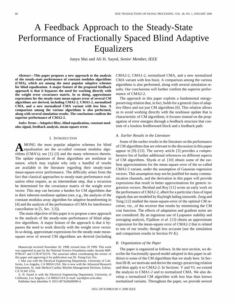
The vectors and are the impulse responses of the two sub-channel blocks shown in Fig. 1. In a similar way, we define thetwo subequalizers

which are the impulse responses of the two subequalizer blocksshown in the same figure. The system in Fig. 1 then correspondsto what is called a multichannel model for a -fractionallyspaced equalizer. This model is well motivated and explained inthe survey article [3].

The output of the combined channel-equalizer systemcan be expressed in terms of the transmitted signal asfollows. Introduce the prewindowed Toeplitzmatrix

......

..... ... ... .

...

and similarly for . Then, define the channelmatrix , the equalizer vector

and the input signal vector

Then, . If we further let and denote theinput signals to the subequalizers and , respectively, anddefine therow input vectors

(1)

(2)

Fig. 1. Multichannel model forT=2-FSE.

and

(3)

then we also have and .

A. Perfect Equalization

An important result for such fractionally spaced equalizersis the following (see, e.g., [3]). Let and denote thepolynomials associated with the even- and odd-indexed sub-channels

Then, it can be shown that if these polynomials do not havecommon zeros, and if , then there exists an equalizer

that leads to an overall channel-equalizer impulse response ofthe form

col (4)

for some constant phase shift , and where the unitentry is in some position , . Equalizers

that result in overall impulse responses of the above formare calledzero-forcingequalizers and will be denoted by .Thus, under such conditions, the output of the channel-equalizersystem will be of the form for some .

The multichannel model of Fig. 1 is the model we are goingto study in future sections. For more general -fractionallyspaced equalizers, we end up with a similar model withsub-channels and subequalizers (see, e.g., [15] and [16]), and theresults in this paper can be readily extended to this context.

B. Constant Modulus Algorithms

We thus see that under a length-and-zero condition, afinite-length FSE can perfectly equalize a noise-free FIRchannel. A blind adaptive equalizer is one that attempts toapproximate a zero forcing equalizer without knowledge ofthe channel impulse response and without direct access to thetransmitted sequence itself. This is achieved by seekingto minimize certain cost functions that are carefully chosen sothat their global minima occur at zero forcing equalizers.

The most popular adaptive blind algorithms are the so-calledconstant modulus algorithms [17], [18]. They are derived as sto-chastic gradient methods for minimizing the cost function

(5)

where denotes the weight vector to be estimated, and the con-stant is suitably chosen in order to guarantee that the globalminima of occur at zero forcing solutions (see, e.g.,[15], [17], and [19]).


In the next two sections, we study the following two variants:CMA2-2 and CMA1-2. In a later section, we study other vari-ants (known as normalized CM algorithms).1

CMA2-2: In this case, we select

(6)

and the update equation for the weight estimates is given by

(7)

with a step-sizeµ and where now, is the outputof the adaptive equalizer. Here, the symboldenotes complexconjugate transposition.

CMA1-2: In this case, we select

(8)

and the update equation for the weight estimates is given by

(9)

Since these algorithms are based on instantaneous approxi-mations of the true gradient vector of the cost function ,the equalizer output need not converge to a zero forcing so-lution of the form due to the presence of gradientnoise. In the following sections, we derive expressions for thesteady-state mean-square error

for adaptive algorithms of the CM class.

III. A N EW APPROACH FORSTEADY-STATE ANALYSIS

As mentioned in the introduction, and as can be seen from theabove equations, the updates for CM algorithms are nonlinearin the weight estimates . This may explain why only a fewresults are available in the literature regarding the steady-stateperformance of this class of algorithms. The difficulty is be-cause for other adaptive schemes (e.g., of the LMS family), itis common to compute steady-state results by first determiningrecursions for the squared weight error energy measuredrelative to some zero-forcing solution, say,(see, e.g., [20]–[23]). This step is a burden for CM algorithmsas well as for several other adaptive schemes, due to their non-linear updates.

Our objective is to propose a new approach for evaluating thesteady-state mean-square error of CM algorithms without re-quiring explicit expressions or recursions for . We moti-vate our approach by first explaining the conventional methodfor evaluating the mean-square error and by showing the diffi-culty it encounters when dealing with adaptive filters with non-linear updates.

1In our notation, we use parenthesis to refer to scalar variables, e.g.,s(i) ory(i) and subscripts to refer to vector quantities, e.g.,w oru . This conventionhelps distinguish between scalar and vector quantities.

A. The Mean-Square Error

Let denote the zero forcing solution that givesfor some . This is guaranteed to exist under

some length-and-zero conditions. Now, due to gradient noise,the adaptive equalizer will yield an output that is distinctfrom . Let denote the resulting (a priori) estimationerror as

One measure of filter performance is the steady-state mean-square error (MSE)

MSE

which is clearly dependent on . It is common in the liter-ature to evaluate this MSE as follows. We first assume that theregression vector is independent of .2 Then, under thisassumption, the above expression for the MSE becomes

MSE Trace (10)

where and, assuming stationarity, .3

It is thus customary to determine the steady-state MSE by firstdetermining the steady-state mean-square deviation (MSD) de-fined by

Trace Trace (11)

This method of evaluation can become a burden for adaptive al-gorithms that involve nonlinear updates in, as is the case withblind adaptive algorithms. We now describe a new approach forevaluating that bypasses the need for studyingand its limit.

B. A Fundamental Energy-Preserving Relation

The approach is based on a fundamental energy-preservingrelation [cf. (20) further ahead], which actually holds for verygeneral adaptive schemes and not just CM algorithms, as ex-plained in [6]. This energy relation was noted and exploited bySayed and Rupp in [26]–[29] in studies on the robustness and

-stability of adaptive filters from a deterministic point of view(see [29]). We review this result below and prepare the notationfor later sections.

Consider a general stochastic algorithm of the form

(12)

where denotes an instantaneous error, anda nonzero(row) regression vector. CM algorithms are a special case of the

2We are not going to impose this condition in our derivation. We are simplyusing it here to demonstrate the common approach in the literature. We mayadd that although not true in general, especially for tapped-delay adaptive filterstructures, this condition is actually a part of certain widely used independenceassumptions in adaptive filter theory [20]. It was shown in [24] and [25], forinstance, that for LMS-type scenarios, and for sufficiently small step- sizes, theconclusions that can be obtained from such independence assumptions tend tomatch reasonably well the real filter performance.

3Since we assume in this paper that the input vectoru is a row vector ratherthan a column vector, its covariance matrix is therefore defined asEu u ratherthanEu u . Our convention of a row vectoru generally simplifies the notationand avoids an overburden of conjugation symbols.


above for different choices of the function . Now, subtractboth sides of (12) from some vector to get the weight errorequation

(13)

where . Define thea priori anda posterioriestimation errors and . Wenow show how to rewrite (13) in terms of the error measures

alone. For this purpose, we note thatif we multiply (13) by from the left, we obtain

(14)

Solving for gives

(15)

so that we can rewrite (13) as

(16)

Rearranging (16) leads to

(17)

If we define

(18)

then by squaring (17), we observe that the following energy re-lation is obtained:

(19)

Interestingly enough, this relation can be obtained by simplyreplacing the terms of (17) by their respective energies; the crossterms cancel out!. We state this result in the form of a theoremfor later reference.

Theorem 1—Energy Relation [26], [27]:Given a genericadaptive algorithm of the form (12), it always holds that

(20)

where .Relation (20) holds forany adaptive algorithm of the form

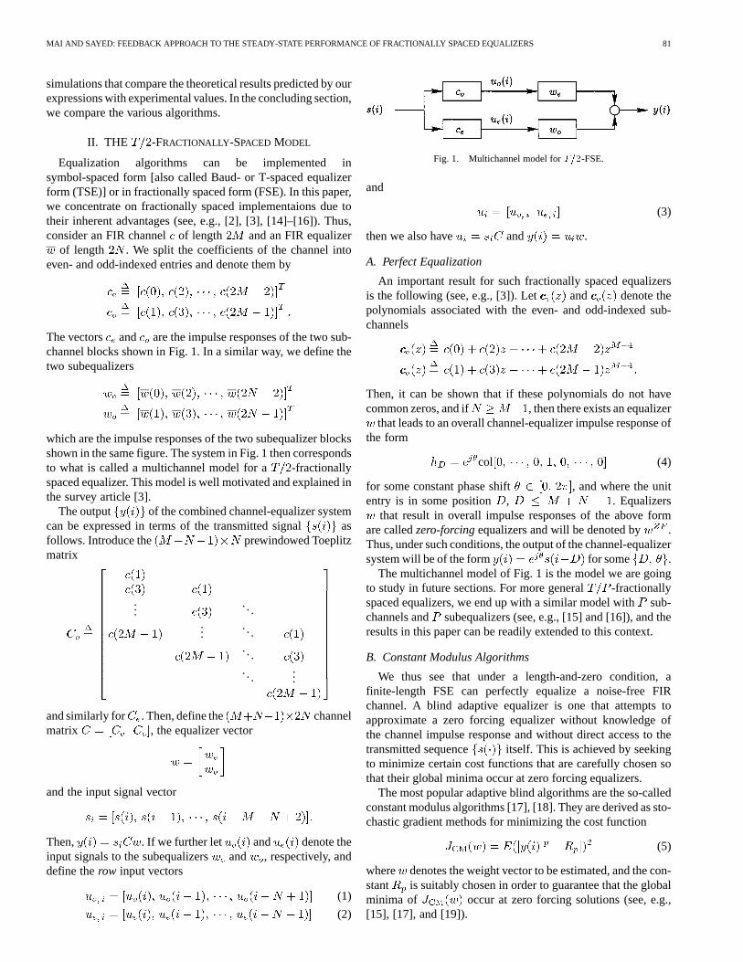
(12); it relates the energies of the weight error vectors attwo successive time instants with the energies of thea prioriand a posteriori errors. No approximations are involved inderiving (20). The relation also has an interesting physicalinterpretation. It establishes that the mapping from the variables

to the variables isenergy preserving. Combining (20) with (14), we see that bothrelations establish the existence of the feedback configurationshown in Fig. 2, where denotes the lossless map from

to , and wheredenotes the unit delay operator. Thus, relation (20) character-izes the energy-preserving property of the feedforward path,whereas relation (14) characterizes the feedback path.

Fig. 2. Lossless mapping and a feedback loop.

C. Significance to MSE Evaluation

We now explain the relevance of the energy relation (20) inthe context of MSE evaluation for CM algorithms. (Applicationsto other classes of adaptive algorithms, in addition to trackinganalyzes, are given in [6]–[8].) By taking expectations of bothsides of (20), we get

(21)

Now, recall that our objective in this paper is to evaluate theMSE of CM algorithms in steady state. We arenot studyingconditions under which an algorithm will tend to steady state,which is a separate and complex issue (especially for nonlinearand time-variant filters). Instead, we want to evaluate what per-formance to expect from an algorithm if it reaches steady state.The convergence to steady state (and, hence, stability) can bestudied by relying on results from averaging analysis and fromso-called ODE methods (e.g., [30]–[32]); these techniques pro-vide tools that allow one to ascertain, under certain conditionson the data, that there exist small enough step sizesµ for whicha filter reaches steady state (see, e.g., [13]).

Thus, assuming filter operation in steady state, we can write

for (22)

[Similar considerations are also common in the steady-stateanalysis of other classes of adaptive algorithms (see, e.g.,[33]).]

Now, with (22), the effect of the weight error vector is can-celed out from (21), and we are reduced to studying only theequality

This equation provides a relation involving only the desired un-known since is itself a function of , as evidencedby (14). Thus, by solving the above equation as , we canobtain an expression for the MSE.

Theorem 2—Identity for MSE Analysis:Consider a genericadaptive algorithm of the form (12). In steady state (as ),when (22) holds, we obtain

(23)


IV. STEADY-STATE ANALYSIS OF CMA2-2

We now demonstrate how the result of Theorem 2, whichholds for generic adaptive schemes of the form (12), can be ap-plied to the CMA2-2 recursion (7). In later sections, we considerother CM algorithms.

The derivation in the sequel relies on some statistical assump-tions (four in total), the introduction of which simplifies theanalysis. Although these assumptions may not hold in general,they are realistic for sufficiently small step sizes and, as we shallsee from several simulations, lead to good fits between our the-oretical results and the simulation results.4 Following each as-sumption, we will provide a brief motivation and justificationfor its use.

A. Two Initial Assumptions

The analysis that follows for CMA2-2 is based on the fol-lowing two assumptions insteady-state( ).

Assumption I.1:The transmitted signal and theestimation error are independent in steady state so that

since is assumed zero mean.This is a reasonable assumption since it essentially re-

quires the estimation error of the equalizer to beinsensitive, in steady-state, to the actual transmitted symbols

. For example, for symbols from a 2-PAM constellation, this means that we are requiring the behavior

(or distribution) of the error , after the equalizer hasconverged to steady state, to be insensitive to whether thepolarity of is 1 or 1.

Assumption I.1 can be replaced by the following two condi-tions, which also enable us to conclude that.

i) In steady state, CMA2-2 converges in the mean to a zeroforcing solution, i.e., the mean of the combined channel-equalizer response converges tocol for some .

ii) and are independent as . That is,in steady state, the equalizer operates independently ofthe transmitted signals. This is a common assumption forsteady-state analysis (see, e.g., [13]).

Assumption I.2:The scaled regressor energy is in-dependent of in steady state.

This assumption requires the scaled energy of the input vectorand not the input vector itself to be independent of the equalizeroutput. The assumption actually becomes realistic for longerfilter lengths and for sufficiently small step sizes. To see this,assume the input sequence is i.i.d., and note that the vari-ance of the quantity will be of the order of (the equal-izer length).5 Hence, if the step-sizeµ is of the order of (orless), then the variance of is of the order of (orless), which decreases with increasing filter length. This means

4Similar assumptions are very common in the adaptive filtering literature forFIR structures, where they are collectively known as the independence assump-tions. As mentioned in a previous footnote, although the independence assump-tions do not hold in general, they still lead to realistic conclusions for sufficientlysmall step sizes [24], [25], [33].

5This is obvious if the individual entries ofu are i.i.d. Some calculationswill show that a similar conclusion holds, in general, when the entries ofu aretaken as the outputs of an FIR channel with i.i.d. input.

that will eventually tend to a constant and can, there-fore, be assumed to be independent of . Note that by thesame argument, we can also assume that is indepen-dent of in steady state. (We may add that an assumptionsimilar to I.2 is also used in [13].)

B. The Case of Real-Valued Data

We start our analysis with the case of real-valued data(e.g., data from a PAM constellation). In the

next section, we consider complex-valued data. It turns out thatthe expressions for the MSE of CMA2-2 are distinct in bothcases, whereas those for CMA1-2 are not.

For real-valued data, the zero forcing responsethat theadaptive equalizer attempts to achieve [cf. (4)] can be of ei-ther form . In the following, wecontinue with the choice , whichyields

A similar analysis holds for the case.

Now, the relation (23) in the CMA2-2 context leads to theequality, for

(24)We will write more compactly (here and throughout the paper)

for

so that (24) becomes, after expanding

This implies that the terms and should coincide. Fromthis equality, we can obtain an approximate expression for thesteady-state MSE as we now verify. (In the argumentbelow, we assume that when the adaptive filter reaches steadystate, the value of is reasonably small.)

Theorem 3—MSE for Real CMA2-2:Consider the CMA2-2recursion (7) with real-valued data . Under As-sumptions I.1 and I.2, it holds that for sufficiently smallµ, thesteady-state MSE can be approximated by

(25)

Proof: We first evaluate . Replacing by , weobtain


Using Assumption I.1 and neglecting for small µ andsmall leads to the approximation .We now evaluate

With Assumption I.2, we can rewrite as in (25a), shown at thebottom of the page. Again, whenµ and are small enough, wecan ignore the term and write

From the equality , we obtain (25).

C. The Case of Complex-Valued Data

The expression for the MSE of CMA2-2 in the complex casediffers from the one we derived above for the real case, as weshall promptly verify.

In the complex case, as in [17], we study signal constellationsthat satisfy the circularity condition

(26)

in addition to the condition , which holdsfor most constellations.

Theorem 4—MSE For Complex CMA2-2:Consider theCMA2-2 recursion (7), and assume complex-valued data

satisfying (26). Under Assumptions I.1 andI.2, and for sufficiently smallµ, the steady-state MSE can beapproximated by

(27)

Proof: Starting with (23), we now obtain

Substituting by , we get

By using (26) and Assumption I.1, the termcan be simplifiedto . Similarly, expanding andusing the same approximations as in the real-valued case, weobtain

Then, from , we get (27). Note that (27) will not benegative because of

and .Comparing the results we get for the real-valued and com-

plex-valued cases, we see that they are similar except for a co-efficient in the denominator expressions (in the real case it isequal to 3 and in the complex case it is equal to 2). Moreover,some useful conclusions can be drawn from these results.

1) The steady-state MSE of CMA2-2 is linearly propor-tional to the step-sizeµ and to the received signalvariance , which agrees with the asymptotic MSEresult for the symbol-spaced (TSE) CM algorithm in [10]and [34]. This property is also similar to that of LMS.

2) For constant modulus signals , we getAccording to (25) and (27), we then obtain .This is also the same as LMS in the absence of noise.

3) For nonconstant modulus signals, the MSE will not bezero, even when there is no system noise. This is be-cause the instantaneous error for CMA2-2 will benonzero, even when . The equalizerweight vector keeps updating itself by a nonvanishingterm and jitters around the mean solution. This propertyis different from LMS, where the instantaneous error willbe equal to zero when the system is perfectly equalized.

D. Simulation Results for CMA2-2

Before proceeding to other CM algorithms, we provide somesimulation results that compare the experimental performancewith the one predicted by the previous theorems. The simula-tions will show than the theoretical values predicted by the ex-pressions in Theorems 3 and 4 match reasonably well the ex-perimental results. The channel considered in this simulation isgiven by . A four-tap FIR filteris used as a -fractionally spaced equalizer.

1) Constant Modulus Signals:A computer simulation wasfirst done for real and constant modulus signals, i.e., for bi-nary data. With a step-size , after 10 000 iterations,CMA2-2 was observed to converge to a zero forcing solutionwith MSE as low as−120 dB, i.e. MSE 10−12, which can beconsidered zero. This result agrees with our analytical result thatthe MSE for constant modulus signals is zero.

(25a)


TABLE IMSE OF CMA2-2 VERSUS STEP-SIZE FOR

6-PAM SIGNALS

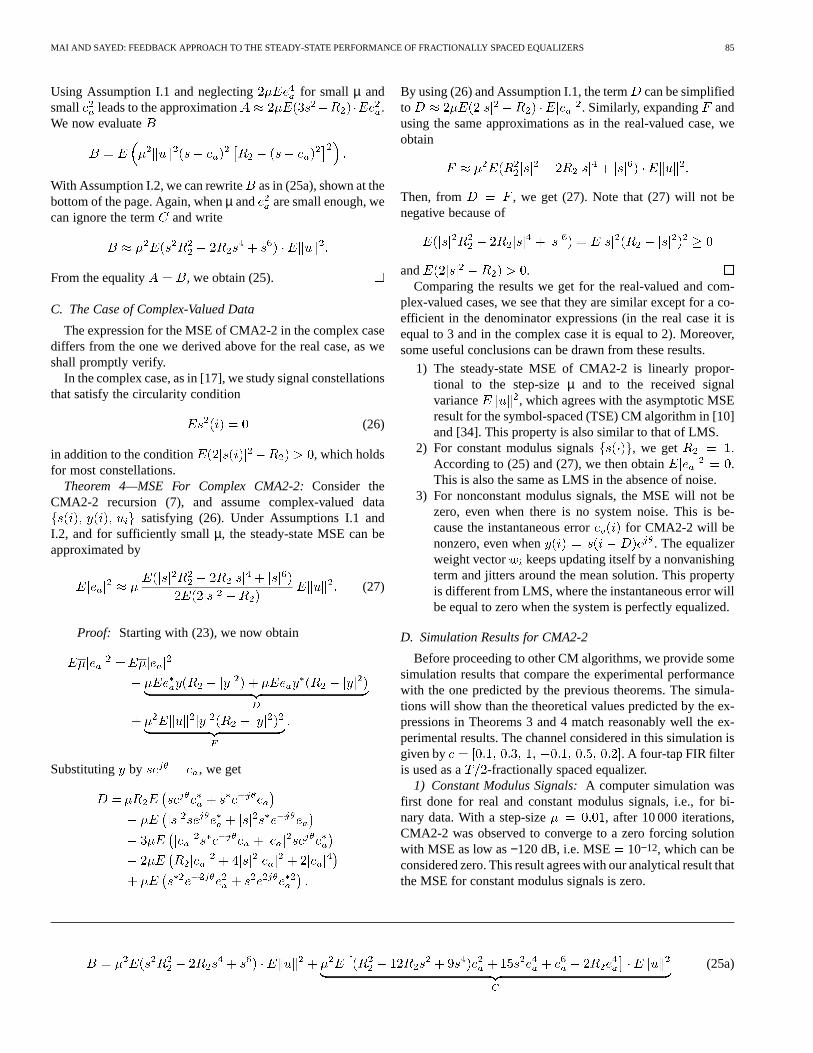
Fig. 3. Experimental and theoretical curves for the steady-state MSE asa function of the step-size, for CMA2-2 with input signals from a 6-PAMconstellation.

2) Real and Nonconstant Modulus Signals:In this simu-lation, the transmitted signal was 6-PAM constellated

with ,, , and . The value of

is the norm of the received signal vector. The value ofwas computed as the average over 3000 realizations of .The first two lines of Table I show the experimental MSE andthe theoretical MSE from Theorem 3, where the value of ex-perimental MSE was obtained as the average over 20 repeatedexperiments. Fig. 3 is a plot of the experimental MSE and thetheoretical MSE versus the step-sizeµ (it also contains one moreMSE curve to be discussed in Section IV-E).

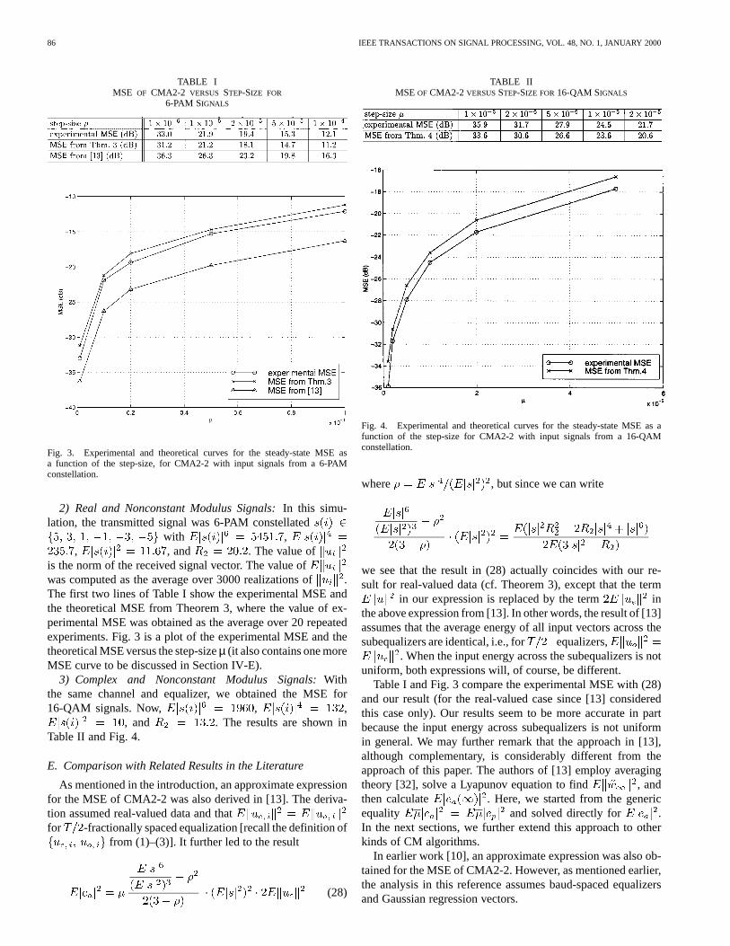
3) Complex and Nonconstant Modulus Signals:Withthe same channel and equalizer, we obtained the MSE for16-QAM signals. Now, , ,

, and . The results are shown inTable II and Fig. 4.

E. Comparison with Related Results in the Literature

As mentioned in the introduction, an approximate expressionfor the MSE of CMA2-2 was also derived in [13]. The deriva-tion assumed real-valued data and thatfor -fractionally spaced equalization [recall the definition of

from (1)–(3)]. It further led to the result

(28)

TABLE IIMSE OF CMA2-2 VERSUSSTEP-SIZE FOR 16-QAM SIGNALS

Fig. 4. Experimental and theoretical curves for the steady-state MSE as afunction of the step-size for CMA2-2 with input signals from a 16-QAMconstellation.

where , but since we can write

we see that the result in (28) actually coincides with our re-sult for real-valued data (cf. Theorem 3), except that the term

in our expression is replaced by the term inthe above expression from [13]. In other words, the result of [13]assumes that the average energy of all input vectors across thesubequalizers are identical, i.e., for equalizers,

. When the input energy across the subequalizers is notuniform, both expressions will, of course, be different.

Table I and Fig. 3 compare the experimental MSE with (28)and our result (for the real-valued case since [13] consideredthis case only). Our results seem to be more accurate in partbecause the input energy across subequalizers is not uniformin general. We may further remark that the approach in [13],although complementary, is considerably different from theapproach of this paper. The authors of [13] employ averagingtheory [32], solve a Lyapunov equation to find , andthen calculate . Here, we started from the genericequality and solved directly for .In the next sections, we further extend this approach to otherkinds of CM algorithms.

In earlier work [10], an approximate expression was also ob-tained for the MSE of CMA2-2. However, as mentioned earlier,the analysis in this reference assumes baud-spaced equalizersand Gaussian regression vectors.


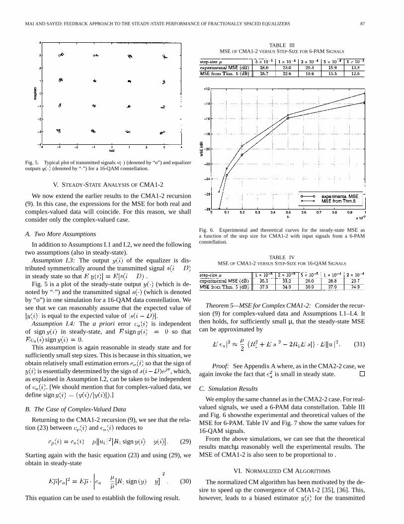
Fig. 5. Typical plot of transmitted signalss(�) (denoted by “o”) and equalizeroutputsy(�) (denoted by “�”) for a 16-QAM constellation.

V. STEADY-STATE ANALYSIS OF CMA1-2

We now extend the earlier results to the CMA1-2 recursion(9). In this case, the expressions for the MSE for both real andcomplex-valued data will coincide. For this reason, we shallconsider only the complex-valued case.

A. Two More Assumptions

In addition to Assumptions I.1 and I.2, we need the followingtwo assumptions (also in steady-state).

Assumption I.3:The output of the equalizer is dis-tributed symmetrically around the transmitted signalin steady state so that .

Fig. 5 is a plot of the steady-state output (which is de-noted by “”) and the transmitted signal (which is denotedby “o”) in one simulation for a 16-QAM data constellation. Wesee that we can reasonably assume that the expected value of

is equal to the expected value of .Assumption I.4:The a priori error is independent

of sign in steady-state, and sign so thatsign .

This assumption is again reasonable in steady state and forsufficiently small step sizes. This is because in this situation, weobtain relatively small estimation errors so that the sign of

is essentially determined by the sign of , which,as explained in Assumption I.2, can be taken to be independentof . [We should mention that for complex-valued data, wedefine sign .]

B. The Case of Complex-Valued Data

Returning to the CMA1-2 recursion (9), we see that the rela-tion (23) between and reduces to

sign (29)

Starting again with the basic equation (23) and using (29), weobtain in steady-state

sign (30)

This equation can be used to establish the following result.

TABLE IIIMSE OF CMA1-2 VERSUSSTEP-SIZE FOR 6-PAM SIGNALS

Fig. 6. Experimental and theoretical curves for the steady-state MSE asa function of the step size for CMA1-2 with input signals from a 6-PAMconstellation.

TABLE IVMSE OF CMA1-2 VERSUSSTEP-SIZE FOR 16-QAM SIGNALS

Theorem 5—MSE for Complex CMA1-2:Consider the recur-sion (9) for complex-valued data and Assumptions I.1–I.4. Itthen holds, for sufficiently smallµ, that the steady-state MSEcan be approximated by

(31)

Proof: See Appendix A where, as in the CMA2-2 case, weagain invoke the fact that is small in steady state.

C. Simulation Results

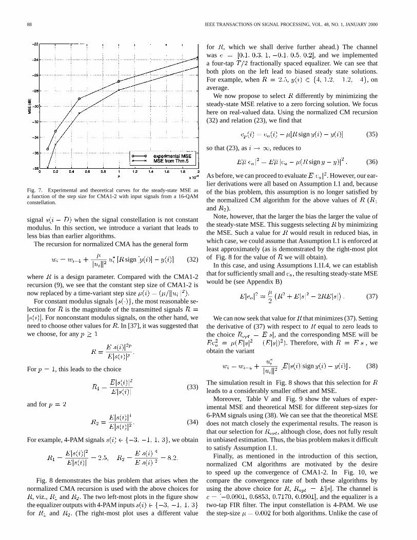
We employ the same channel as in the CMA2-2 case. For real-valued signals, we used a 6-PAM data constellation. Table IIIand Fig. 6 showsthe experimental and theoretical values of theMSE for 6-PAM. Table IV and Fig. 7 show the same values for16-QAM signals.

From the above simulations, we can see that the theoreticalresults matchµ reasonably well the experimental results. TheMSE of CMA1-2 is also seen to be proportional to .

VI. NORMALIZED CM ALGORITHMS

The normalized CM algorithm has been motivated by the de-sire to speed up the convergence of CMA1-2 [35], [36]. This,however, leads to a biased estimator for the transmitted


Fig. 7. Experimental and theoretical curves for the steady-state MSE asa function of the step size for CMA1-2 with input signals from a 16-QAMconstellation.

signal when the signal constellation is not constantmodulus. In this section, we introduce a variant that leads toless bias than earlier algorithms.

The recursion for normalized CMA has the general form

sign (32)

where is a design parameter. Compared with the CMA1-2recursion (9), we see that the constant step size of CMA1-2 isnow replaced by a time-variant step size .

For constant modulus signals , the most reasonable se-lection for is the magnitude of the transmitted signals

. For nonconstant modulus signals, on the other hand, weneed to choose other values for. In [37], it was suggested thatwe choose, for any

For , this leads to the choice

(33)

and for

(34)

For example, 4-PAM signals , we obtain

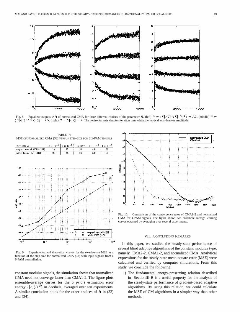
Fig. 8 demonstrates the bias problem that arises when thenormalized CMA recursion is used with the above choices for

, viz., and . The two left-most plots in the figure showthe equalizer outputs with 4-PAM inputsfor and . (The right-most plot uses a different value

for , which we shall derive further ahead.) The channelwas , and we implementeda four-tap fractionally spaced equalizer. We can see thatboth plots on the left lead to biased steady state solutions.For example, when , , onaverage.

We now propose to select differently by minimizing thesteady-state MSE relative to a zero forcing solution. We focushere on real-valued data. Using the normalized CM recursion(32) and relation (23), we find that

sign (35)

so that (23), as , reduces to

sign (36)

As before, we can proceed to evaluate . However, our ear-lier derivations were all based on Assumption I.1 and, becauseof the bias problem, this assumption is no longer satisfied bythe normalized CM algorithm for the above values of(and ).

Note, however, that the larger the bias the larger the value ofthe steady-state MSE. This suggests selectingby minimizingthe MSE. Such a value for would result in reduced bias, inwhich case, we could assume that Assumption I.1 is enforced atleast approximately (as is demonstrated by the right-most plotof Fig. 8 for the value of we will obtain).

In this case, and using Assumptions I.1I.4, we can establishthat for sufficiently small and , the resulting steady-state MSEwould be (see Appendix B)

(37)

We can now seek that value forthat minimizes (37). Settingthe derivative of (37) with respect to equal to zero leads tothe choice , and the corresponding MSE will be

. Therefore, with , weobtain the variant

sign (38)

The simulation result in Fig. 8 shows that this selection forleads to a considerably smaller offset and MSE.

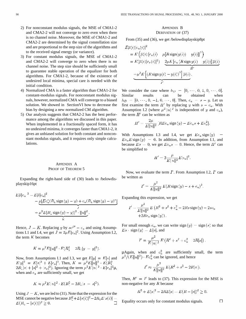
Moreover, Table V and Fig. 9 show the values of exper-imental MSE and theoretical MSE for different step-sizes for6-PAM signals using (38). We can see that the theoretical MSEdoes not match closely the experimental results. The reason isthat our selection for , although close, does not fully resultin unbiased estimation. Thus, the bias problem makes it difficultto satisfy Assumption I.1.

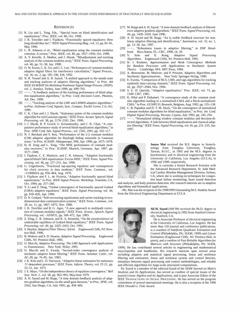
Finally, as mentioned in the introduction of this section,normalized CM algorithms are motivated by the desireto speed up the convergence of CMA1-2. In Fig. 10, wecompare the convergence rate of both these algorithms byusing the above choice for , . The channel is

, and the equalizer is atwo-tap FIR filter. The input constellation is 4-PAM. We usethe step-size for both algorithms. Unlike the case of


Fig. 8. Equalizer outputsy(i) of normalized CMA for three different choices of the parameterR. (left) R = (Ejs(i)j =Ejs(i)j ) = 8:2. (middle)R =(Ejs(i)j =Ejs(i)j) = 2:5. (right)R = Ejs(i)j = 2. The horizontal axis denotes iteration time while the vertical axis denotes amplitude.

TABLE VMSE OF NORMALIZED CMA (38) VERSUSSTEP-SIZE FORSIX-PAM SIGNALS

Fig. 9. Experimental and theoretical curves for the steady-state MSE as afunction of the step size for normalized CMA (38) with input signals from a6-PAM constellation.

constant modulus signals, the simulation shows that normalizedCMA need not converge faster than CMA1-2. The figure plotsensemble-average curves for thea priori estimation errorenergy in decibels, averaged over ten experiments.A similar conclusion holds for the other choices ofin (33)and (34).

Fig. 10. Comparison of the convergence rates of CMA1-2 and normalizedCMA for 4-PAM signals. The figure shows two ensemble-average learningcurves obtained by averaging over several experiments.

VII. CONCLUDING REMARKS

In this paper, we studied the steady-state performance ofseveral blind adaptive algorithms of the constant modulus type,namely, CMA2-2, CMA1-2, and normalized CMA. Analyticalexpressions for the steady-state mean-square error (MSE) werecalculated and verified by computer simulations. From thisstudy, we conclude the following.

1) The fundamental energy-preserving relation describedin SectionIII-B is a useful property for the analysis ofthe steady-state performance of gradient-based adaptivealgorithms. By using this relation, we could calculatethe MSE of CM algorithms in a simpler way than othermethods.


2) For nonconstant modulus signals, the MSE of CMA1-2and CMA2-2 will not converge to zero even when thereis no channel noise. Moreover, the MSE of CMA1-2 andCMA2-2 are determined by the signal constellation sizeand are proportional to the step size of the algorithms andto the received signal energy (or variance).

3) For constant modulus signals, the MSE of CMA1-2and CMA2-2 will converge to zero when there is nochannel noise. The step size should be sufficiently smallto guarantee stable operation of the equalizer for bothalgorithms. For CMA1-2, because of the existence ofundesired local minima, special care is needed with theinitial condition.

4) Normalized CMA is a faster algorithm than CMA1-2 forconstant-modulus signals. For nonconstant modulus sig-nals, however, normalized CMA will converge to a biasedsolution. We showed in SectionVI how to decrease thebias by designing a new normalized CM algorithm.

5) Our analysis suggests that CMA2-2 has the best perfor-mance among the algorithms we discussed in this paper.When implemented in a fractionally spaced form, it hasno undesired minima, it converges faster than CMA1-2, itgives an unbiased solution for both constant and noncon-stant modulus signals, and it requires only simple calcu-lations.

APPENDIX APROOF OFTHEOREM 5

Expanding the right-hand side of (30) leads to /belowdis-playskip16pt

sign sign

sign

Hence, . Replacing by and using Assump-tions I.1 and I.4, we get . Using Assumption I.2,the term becomes

Now, from Assumptions I.1 and I.3, we get and. Then,

. Ignoring the term µ,when and are sufficiently small, we get

Using , we are led to (31). Note that the expression for theMSE cannot be negative because

.

APPENDIX BDERIVATION OF (37)

From (35) and (36), we get /belowdisplayskip8pt

sign

sign

sign

We consider the case where .Similar results can be obtained when

. Then, . Let usfirst examine the term by replacing with . WithAssumption I.2 (where is independent of and ),the term can be written as

sign

With Assumptions I.3 and I.4, we get signsign In addition, from Assumption I.1, and

because , we get . Hence, the term canbe simplified to

Now, we evaluate the term. From Assumption I.2, canbe written as

sign

Expanding this expression, we get

sign

sign

For small enough , we can write sign sign so thatsign , and

µAgain, when and are sufficiently small, the termcan be ignored, and hence

Then, leads to (37). This expression for the MSE isnon-negative for any because

Equality occurs only for constant modulus signals.


REFERENCES

[1] R. Liu and L. Tong, Eds., “Special issue on blind identification andequalization,”Proc. IEEE, vol. 86, Oct. 1998.

[2] J. R. Treichler and I. Fijalkow, “Fractionally spaced equalizers: Howlong should they be?,”IEEE Signal Processing Mag., vol. 13, pp. 65–81,May 1996.

[3] C. R. Johnsonet al., “Blind equalization using the constant moduluscriterion: A review,”Proc. IEEE, vol. 86, pp. 1927–1950, Oct. 1998.

[4] A. V. Keerthi, A. Mathur, and J. Shynk, “Misadjustment and trackinganalysis of the constant modulus array,”IEEE Trans. Signal Processing,vol. 46, pp. 51–58, Jan. 1998.

[5] O. W. Kwon, C. K. Un, and J. C. Lee, “Performance of constant modulusadaptive digital filters for interference cancellation,”Signal Process.,vol. 26, no. 2, pp. 185–196, Feb. 1992.

[6] N. R. Yousef and A. H. Sayed, “A unified approach to the steady-stateand tracking analyzes of adaptive filtering algorithms,” inProc. 4thIEEE-EURASIP Int.Workshop Nonlinear Signal Image Process. (NSIP),vol. 2, Antalya, Turkey, June 1999, pp. 699–703.

[7] , “A feedback analysis of the tracking performance of blind adap-tive equalization algorithms,” inProc. Conf. Decision Contr., Phoenix,AZ, Dec. 1999.

[8] , “Tracking analysis of the LMF and LMMN adaptive algorithms,”in Proc. Asilomar Conf. Signals, Syst., Comput., Pacific Grove, CA, Oct.1999.

[9] C. K. Chan and J. J. Shynk, “Stationary points of the constant modulusalgorithm for real Gaussian signals,”IEEE Trans. Acoust. Speech, SignalProcessing, vol. 38, pp. 2176–2181, Dec. 1990.

[10] J. J. Shynk, R. P. Gooch, G. Krisnamurthy, and C. K. Chan, “A com-parative performance study of several blind equalization algorithms,” inProc. SPIE Conf. Adv. Signal Process., vol. 1565, 1991, pp. 102–117.

[11] N. J. Bershad and S. Roy, “Performance of the 2-2 constant modulus(CM) adaptive algorithm for Rayleigh fading sinusoids in Gaussiannoise,” inProc. ICASSP, Albuquerque, NM, Apr. 1990, pp. 1675–1678.

[12] H. H. Zeng and L. Tong, “The MSE performance of constant mod-ulus receivers,” inProc. ICASSP, Munich, Germany, Apr. 1997, pp.3577–3580.

[13] I. Fijakow, C. E. Manlove, and C. R. Johnson, “Adaptive fractionallyspaced blind CMA equalization: Excess MSE,”IEEE Trans. Signal Pro-cessing, vol. 46, pp. 227–231, Jan. 1998.

[14] G. Ungerboeck, “Fractional tap-spacing equalizer and consequencesfor clock recovery in data modems,”IEEE Trans. Commun., vol.–COMM24, pp. 856–864, Aug. 1976.

[15] I. Fijalkow and F. L. de Victoria, “Adaptive fractionally spaced blindequalization,” inProc. IEEE Signal Process. Workshop, Yosemite, CA,Oct. 1994, pp. 257–260.

[16] Y. Li and Z. Ding, “Global convergence of fractionally spaced Godard(CMA) adaptive equalizers,”IEEE Trans. Signal Processing, vol. 44,pp. 818–826, Apr. 1996.

[17] D. N. Godard, “Self-recovering equalization and carrier tracking in two-dimensional data communication systems,”IEEE Trans. Commun., vol.28, no. 11, pp. 1867–1875, Nov. 1980.

[18] J. R. Treichler and B. G. Agee, “A new approach to multipath correc-tion of constant modulus signals,”IEEE Trans. Acoust., Speech, SignalProcessing, vol. –ASSP31, pp. 349–472, Apr. 1983.

[19] Z. Ding, C. R. Johnson, and R. A. Kennedy, “On the (non)existence ofundesirable equilibria of Godard blind equalizers,”IEEE Trans. SignalProcessing, vol. 40, pp. 2425–2432, Oct. 1992.

[20] S. Haykin,Adaptive Filter Theory, 3rd ed. Englewood Cliffs, NJ: Pren-tice-Hall, 1996.

[21] B. Widrow and S. D. Stearns,Adaptive Signal Processing. EnglewoodCliffs, NJ: Prentice-Hall, 1985.

[22] O. Macchi,Adaptive Processing: The LMS Approach with Applicationsin Transmission. New York: Wiley, 1995.

[23] O. Macchi and E. Eweda, “Second-order convergence analysis ofstochastic adaptive linear filtering,”IEEE Trans. Automat. Contr., vol.AC-28, pp. 76–85, Jan. 1983.

[24] J. K. Kim and L. D. Davisson, “Adaptive linear estimation for stationaryM -dependent processes,”IEEE Trans. Inform. Theory, vol. IT-21, pp.23–31, Jan. 1975.

[25] J. E. Mazo, “On the independence theory of equalizer convergence,”BellSyst. Tech. J., vol. 58, pp. 963–993, May/June 1979.

[26] A. H. Sayed and M. Rupp, “A time domain feedback analysis of adap-tive gradient algorithms via the small gain theorem,” inProc. SPIE, vol.2563, San Diego, CA, July 1995, pp. 458–469.

[27] M. Rupp and A. H. Sayed, “A time-domain feedback analysis of filtered-error adaptive gradient algorithms,”IEEE Trans. Signal Processing, vol.44, pp. 1428–1439, June 1996.

[28] A. H. Sayed and M. Rupp, “Anl -stable feedback structure for non-linear adaptive filtering and identification,”Automatica, vol. 33, no. 1,pp. 13–30, Jan. 1997.

[29] , “Robustness issues in adaptive filtering,” inDSP Hand-book. Boca Raton, FL: CRC, 1998, ch. 20.

[30] V. Solo and X. Kong, Adaptive Signal ProcessingAlgorithms. Englewood Cliffs, NJ: Prentice-Hall, 1995.

[31] H. J. Kushner, Approximation and Weak Convergence Methodsfor Random Processes with Applications to Stochastic SystemTheory. Cambridge, MA: MIT Press, 1984.

[32] A. Benveniste, M. Metivier, and P. Priouret,Adaptive Algorithms andStochastic Approximations. New York: Springer-Verlag, 1990.

[33] E. Eweda, “Comparison of RLS, LMS, and sign algorithms for trackingrandomly time-varying channels,”IEEE Trans. Signal Processing, vol.42, pp. 2937–2944, Nov. 1994.

[34] S. U. H. Quershi, “Adaptive equalization,”Proc. IEEE, vol. 73, pp.1349–1387, 1985.

[35] K. Hilal and P. Duhamel, “A convergence study of the constant mod-ulus algorithm leading to a normalized-CMA and a block-normalized-CMA,” in Proc. EUSIPCO, Brussels, Belgium, Aug. 1992, pp. 135–138.

[36] C. B. Papadias and D. T. M. Slock, “On the convergence of normalizedconstant modulus algorithms for blind equalization,” inProc. Int. Conf.Digital Signal Processing, Nicosia, Cyprus, July 1993, pp. 245–250.

[37] , “Normalized sliding window constant modulus and decision-di-rected algorithms: A link between blind equalization and classical adap-tive filtering,” IEEE Trans. Signal Processing, vol. 45, pp. 231–235, Jan.1997.

Junyu Mai received the B.S. degree in biotech-nology from Tsinghua University, Tsinghua,Taiwan, R.O.C., in 1995 and the M.S. degrees inbiochemistry and in electrical engineering from theUniversity of California, Los Angeles (UCLA), in1996 and 1998, respectively.

She is currently a Senior Research Scientist withthe Advanced Research Department, St. Jude Med-ical Cardiac Rhythm Management Division, Sylmar,CA, where she is working on techniques for conges-tive heart failure monitoring, heart sound detection

and analysis, and body position detection. Her research interests are in adaptivealgorithms and biomedical applications.

–Ms. Mai was the recipient of the 19981999 Outstanding M.S. Student Awardfrom the Electrical Engineering Department at UCLA.

Ali H. Sayed (SM’99) received the Ph.D. degree inelectrical engineering in 1992 from Stanford Univer-sity, Stanford, CA.

He is Associate Professor of electrical engineeringat the University of California, Los Angeles. He hasmore than 120 journal and conference publications,is a coauthor ofIndefinite Quadratic Estimation andControl (Philadelphia, PA: SIAM, 1999) andLinearEstimation(Englewood Cliffs, NJ: Prentice-Hall, inpress), and a coeditor ofFast Reliable Algorithms forMatrices with Structure(Philadelphia, PA: SIAM,

1999). He has contributed several articles to engineering and mathematicalencyclopedias and handbooks. His research interests span several areasincluding adaptive and statistical signal processing, linear and nonlinearfiltering and estimation, linear and nonlinear system and control theories,interplays between signal processing and control methodologies, and reliableand efficient algorithms for large-scale structured computations.

Dr. Sayed is a member of the editorial board of theSIAM Journal on MatrixAnalysis and Its Applications, has served as coeditor of special issues of thejournalLinear Algebra and Its Applications, and is past Associate Editor of theIEEE TRANSACTIONS ONSIGNAL PROCESSING. He has served on the programcommittees of several international meetings. He is also a recipient of the 1996IEEE Donald G. Fink Award.

A feedback approach to the steady-state performance of fractionally spaced blind adaptive equalizers

Documents