A Fast Third-Step Second-Order Explicit Numerical Approach ...

arX

iv:2

206.

0502

2v1

[ec

on.G

N]

3 J

un 2

022

A Fast Third-Step Second-Order Explicit Numerical Approach To

Investigating and Forecasting The Dynamic of Corruption And

Poverty In Cameroon

Eric Ngondiep

1Department of Mathematics and Statistics, College of Science, Imam Mohammad Ibn SaudIslamic University (IMSIU), 90950 Riyadh 11632, Saudi Arabia.

2Hydrological Research Centre, Institute for Geological and Mining Research, 4110 Yaounde-Cameroon.

Email addresses: [email protected]/[email protected]

Abstract. This paper constructs a third-step second-order numerical approach for solving a mathemat-ical model on the dynamic of corruption and poverty. The stability and error estimates of the proposedtechnique are analyzed using the L2-norm. The developed algorithm is at less zero-stable and second-orderaccurate. Furthermore, the new method is explicit, fast and more efficient than a large class of numericalschemes applied to nonlinear systems of ordinary differential equations and can serve as a robust tool forintegrating general systems of initial-value problems. Some numerical examples confirm the theory and alsoconsider the corruption and poverty in Cameroon.

Keywords: mathematical model on dynamic of corruption and poverty, a third-step explicitnumerical method, stability analysis, convergence accurate, numerical examples.

AMS Subject Classification (MSC). 65M12, 65M06.

1 Introduction and motivation

Poverty and corruption problems remain the core development challenge on a global level. Poverty is definedas the failure to attain a minimum level of well-being and it is the main issue at which people are confronted.In the literature [25, 55, 48], many authors have demonstrated that poverty and inequality have still beenthe forefront of all economic problems. The required consumption per capita condition to ensure a minimumlife standardize is called poverty line and it is computed by the Cost of Basic Needs (CBN) technique. TheCBN approach is used by a large class of researchers to estimate the poverty line in many countries [47].Corruption is directly related to poverty and it can be observed as one of the major factor of poverty and abarrier to successfully eradicate it.

Transparency International (TI) has defined corruption as the misuse of entrusted power for private gainwhereas the Worth Bank (WB) considered the corruption as the abuse of public office for private benefit. Inseveral nations, the phenomenon of corruption has negative impacts on economy and society. Specifically,it is a powerful instrument to destroy a society, can be considered as a cancer to political development, eco-nomic and social activities. Furthermore, corruption greatly improves income inequalities by sharing powerimbalances in poor countries. In almost all the sectors, mainly the public sector, corruption deepens povertyby delaying and diverting economic growth and productive programs such as: health care and education atthe expense of a wide class of capital intensive projects that should suggest better opportunities to overcomeillegal expenditures. The corruption deals in different levels: from the high levels corruption which concernsthe highest level of national government to the pretty one, that is, the exchange of very small amounts ofmoney or the granting of minors favors by those in lower positions. Thus, the society wants to uphold the

1

value of a Man for what he is and not what he has. Though there exists a strong relationship between cor-ruption and poverty, it has been observed that policy recommendation to combating corruption and povertyhas failed. However, Researchers have demonstrated that fighting corruption is a good remedy to reducepoverty [2, 11, 19].

In Cameroon, poverty is much more than just having enough money to meet basic needs including: food,clothing and shelter. More precisely, poverty includes: hunger, lack of shelter, being sick and unable to seea physician, unemployment, fear for the future and living one day at time. In addition, in some rural areaschildren cannot go to school because of worst life conditions and thus are incapable to read and write. Since1985, the country has developed a new poverty line of 36000 FCFA (equivalent of US $65, 5) per monthwhich does not allow people to access minimum consumption conditions for a standard sized household forbasic needs mentioned above. Thus, a large class of individuals live in extreme poverty. For more detailsabout extreme poverty and corruption in Cameroon, we refer the readers to [21]. For some years now, amajority of cameroonians have shown very little interest in studying and serving in the country. This greatlack of motivation is partly due to unemployment, misery and very low salaries which since 1993 are wellhalf below the poverty line: case of private teachers of primary and secondary schools, caretaker, etc...

From 1978 to 1983, the poverty line developed in the country was indicating that less than 1% of the pop-ulation was considered poor and after this period, the government ignored this restriction and the povertyrate grew. In many Cameroon hospitals such as: Yaounde central hospital, Douala laquintine hospital,Biyem-Assi district hospital, etc..., patients and newborn babies dead almost every day because no nurseor physician can take care of them. They are extremely poor and not are capable to pay the investigationfees. Furthermore, since 2016 some people in renting in Yaounde moved house for a new area, so called Elig-Essomballa, where they lived without electricity during more than a year. After submitting many requeststo the department in charge of energy (ENEO) without getting a solution, individuals with modest incomesrepresenting 30% of the population in the district, considered this problem as their own project whereasthose living in high level of misery were still in obscurity because unable to contribute to the project even assmall as possible. From 2019 to date, although nothing is done regarding electricity in the area, the energydepartment obliged persons using the project initiated in 2018 to subscribe for an electrical meter in ENEOagency and to pay the consumption every month. In addition, in March 2022 a union of teachers for publicschools, so called ”One has suffered too much” stopped teaching during more than a month after submittingseveral requests to Cameroon government regarding valuable problems related to their profession, which lastfor more than a decade (the majority of them have worked during many years without salaries, housing,career prospects,...). In Cameroon, there is a direct correlation between poverty and corruption and gen-eralized poverty is one of the main social causes of corruption. Regardless of the scope of corruption, suchacts undetermine the development of civil society and exacerbate poverty, especially when public resourcesthat should be used to improve people’s life are abused or mismanaged by public officials [21]. Here, thecharacteristics of the corruption are: bribery, conflict of interest, nepotism, illicit financial flow as definedin [44], electoral financing, financial leakage, embezzlement, tax evasion, budget process, high levels corrup-tion (presidential and parliamentary elections), bureaucratic corruption, false account and fraud [51]. Thisphenomenon has plagued the whole components of the country, particularly: Judicial, Military, Financial,Health, Educational and other departments. Furthermore, Cameroon has topped twice the list of most cor-rupt countries in the world in 1998-1999 [49]. Although the government has put in place some Institutions(French Acronym (CONAC), Supreme State Audit (SSA), National Anti-Corruption Commission (NACC),Inter Employer Grouping of Cameroon (GICAM), Business Coalition Against Corruption (BCAC) and Spe-cial Criminal Court (SCC)) to fight against corruption in both public and private sectors, perception of thisphenomenon continues to affect people trust in public services and justice systems. For instance, the actualpresident of republic did forty years as head of state and several of his collaborators occupied the post ofminister during at least twenty five years. These public servants are from eighty years old to ninety. Formore details, we refer the readers to [5, 1, 9, 18, 24, 45, 50, 52]. In this country of central Africa, corruptionlies in the field of dangerous infectious diseases which are described as a pandemic. For most citizens theanti-corruption campaign has been merely a wasted effort since the government does not take any measuresagainst the corrupted and corrupters. There is a general feeling that corruption and in particular high-levels corruption has been institutionalized to maintaining the same person as ”lifetime” head of state [18].

2

Furthermore, the report [8] suggested that more than 14.7 billion FCFA (i.e., $26.73 million) has been lostby the State as a result of mismanagement and corruption. In this report, it is established that the mostcorrupt public services in Cameroon are mainly the ministry of finance (treasury, taxes, customs, centraland decentralized services, etc...), public security (roadside check, establishment of passports and nationalidentity cards, police custody, etc...), ministry of public contracts (recruitment, appointment of employees,career prospects,...), ministry of justice (corruption of magistrates and slowness in rendering justice,...) andministry of defense (appointment of staff,...) [8, 9]. In [7] it is established that more than 4700 billion FCFA(approximately, US $8.1 billion) for about 20% of the Gross Domestic Product (GDP) has been embezzledin the last decades and stashed in foreign banks by many high ranking members of government. However,no deeply study has been carried out to estimate the exact amount embezzled in the Cameroon budgetsince its year of independence, 1960. This situation widely delayed and diverted economic growth and socialdevelopment. Thus, a serious combat against corruption should highly improve the poverty reduction process.

In the literature [25, 48, 15, 26, 27], a wide set of scientists have developed efficient numerical techniquesin an approximate solution of mathematical models of the dynamic of poverty, corruption and infectiousdiseases. This class of model lies in the field of complex systems of ordinary differential equations (ODEs).The difficulties in computing exact solutions to such types of complex systems are closely related to thosein solving certain class of nonlinear partial differential equations (PDEs) [31, 36, 28, 42, 32, 30, 39]. Forsuch classes of problems, several authors have analyzed a broad range of statistical and numerical methodsin approximate solutions. For more details, the readers can consult the works discussed in [25, 41, 33, 55,35, 26, 38, 48, 34, 43, 37, 4, 29] and references therein. In this paper, we develop an efficient third-stepsecond-order convergent explicit numerical approach for solving a system of nonlinear ODEs modeled by thedynamic of poverty and corruption. The proposed numerical scheme is stable for any value of the initialcondition, second-order convergence, fast and more efficient than a large class of numerical techniques widelystudied in the literature for solving similar problems [25, 55, 15, 3, 6, 10, 27]. The numerical experiments areperformed using the data coming from Cameroon, a country located in central Africa and where corruptioncan be compared to a ”pathology” and poverty reached the half of poverty line [54, 47]. We recall that thispaper deals with a computed solution of the mathematical model on the dynamic of corruption and poverty.Particularly, we are interested in the following four items:

i. Mathematical reformulation on the dynamic of corruption and poverty,

ii. detailed description of the third-step second-order explicit numerical scheme applied to problem men-tioned in item i),

iii. stability analysis and error estimates of the developed approach,

iv. a large set of numerical examples which validate the theoretical studies and also considers the particularcase of corruption and poverty in Cameroon.

The remainder of the work is the following: Section 2 deals with the mathematical model on the dy-namic of corruption and poverty. In Section 3, we develop the third-step explicit numerical technique inan approximate solution of the considered problem. The stability together with the error estimates of thenew algorithm are deeply analyzed in Section 4 whereas a large class of numerical evidences are discussedin Section 5. Finally, Section 6 considers the general conclusions and presents future works.

2 Mathematical model on the dynamic of corruption and poverty

This section deals with a nonlinear model describing the dynamic of poverty and corruption. The populationis assumed to be homogeneous (so that the spatial variable is neglected) divided into five compartments asfollows:

• y1(t): Susceptible persons: the people in this class are never involved in any corruption which couldimpact the economic growth of the country,

• y2(t): Corrupt people: persons who are convicted in corrupt practices and are able to convince asusceptible individual to become corrupt,

3

• y3(t): Poverty class: individuals whose monthly incomes are below the poverty line,

• y4(t): Prosecuted/imprisoned individuals: people who are involved in corrupt acts and jailed for aspecific period of time. During this period, they can neither be involved in any corrupt practices norinfluence others,

• y5(t): Honest persons: individuals who could never be corrupted even whether their life conditionsbecome bad.

With the above tools, we should analyze a mathematical model on the dynamic of poverty and corruptiondescribed in [14] by the following system of nonlinear ordinary differential equations

y1(t)

dt= θ −

1

N(α1y1y2 + α2y1y3)(t) − (γ + σ)y1(t), on I = (t0, T ), (1)

y2(t)

dt=

1

N(α1y1y2 + r2y2y3)(t)− (γ + b1 + τ + r1)y2(t) + ρ(1− µ)y4(t), on I = (t0, T ), (2)

y3(t)

dt=

1

N(α2y1y3 − r2y2y3)(t) + r1y2(t)− (γ + b2)y3(t), on I = (t0, T ), (3)

y4(t)

dt= τy2(t)− [ρ(1− µ) + ρµ+ γ]y4(t), on I = (t0, T ), (4)

y5(t)

dt= σy1(t) + b1y2(t) + b2y3(t) + ρµy4(t)− γy5(t), on I = (t0, T ), (5)

subjects to initial condition

y1(t0) = y01 , y2(t0) = y02 , y3(t0) = y03 , y4(t0) = y04 , y5(t0) = y05 , (6)

where θ and γ are the recruitment rate into the susceptible population and the death removal rate respec-tively, 1/ρ is the average period prosecuted persons spend in prison, ρµ represents the transition rate fromimprisoned to honest, ρ(1 − µ) designates the transition rate from jailed to corrupt, p1 and p2 indicate thecorruption transmission probability per contact and the poverty transmission probability per contact respec-tively, β1 and β2 denote both effort rates against corruption and poverty respectively, α1 = p1(1 − β1) andα2 = p2(1− β2) are the effective corruption contact rate and the effective poverty contact rate respectively,r1 and r2 represent the rates at which both corrupt individuals and poor persons become poor and corruptrespectively, τ means the proportion of corrupt individuals prosecuted and jailed, b1, b2 and σ indicate theproportion of corrupt persons, poor individuals and susceptible people, respectively, that become honestpersons and N is the size of the population in the considered country (for example: Cameroon). Withoutloss of the generality, we assume in this work that for a fixed period of time, the number of births equals thenumber of deaths. This assumption suggests that N is constant. Furthermore, y0i , i = 1, 2, ..., 5, denote theinitial data. It is worth noticing to mention that when the function y3 vanishes on the interval I = (t0, T ),the initial-value problem (1)-(6) provides the only model for dynamic of corruption, which is defined as

y1(t)

dt= θ − (γ + σ)y1(t)−

1

Nα1y1(t)y2(t), on I,

y2(t)

dt= −(γ + b1 + τ + r1)y2(t) +

1

Nα1y1(t)y2(t) + ρ(1− µ)y4(t), on I,

y4(t)

dt= τy2(t)− [ρ(1− µ) + ρµ+ γ]y4(t), on I,

y5(t)

dt= σy1(t) + b1y2(t) + ρµy4(t)− γy5(t), on I,

subjects to initial condition

y1(t0) = y01 , y2(t0) = y02 , y4(t0) = y04 , y5(t0) = y05 .

4

However, the aim of this paper is not to focus the study on the only model of corruption. We introduce thefollowing functions and vector functions:

y : I → R5

t 7→ (y1(t), ..., y5(t)) ,

and

F : I × R5 → R

5

(t, y) 7→ (F1(t, y), ..., F5(t, y)) ,

where for i = 1, 2, ..., 5, Fi : I × R5 → R are defined as

F1(t, y) = θ −1

N(α1y1y2 + α2y1y3)(t)− (γ + σ)y1(t), (7)

F2(t, y) =1

N(α1y1y2 + r2y2y3)(t)− (γ + b1 + τ + r1)y2(t) + ρ(1− µ)y4(t), (8)

F3(t, y) =1

N(α2y1y3 − r2y2y3)(t) + r1y2(t)− (γ + b2)y3(t), (9)

F4(t, y) = τy2(t)− [ρ(1− µ) + ρµ+ γ]y4(t), (10)

F5(t, y) = σy1(t) + b1y2(t) + b2y3(t) + ρµy4(t)− γy5(t). (11)

Plugging equations (1)-(11) to obtain the following system of ODEs

dy

dt= F (t, y), on I = (t0, T ), (12)

with initial conditiony(t0) = y0, (13)

where dydt = (dy1dt , ...,

dy5dt ) and y

0 = (y01 , ..., y05).

Now, it follows from equations (7)-(11) that the functions Fi and their partial derivatives are continuouslydifferentiable on the strip S = {(t, y), t ∈ [t0, T ], y ∈ R5}, whereas the partial derivatives ∂yjFi are notbounded on this domain. By the Henrici result [22], the initial-value problem (1)-(6) has a unique solutiony(t) defined in a certain neighborhood I(t0) ⊂ [t0, T ] of the initial datum t0. Since the system of nonlinear

equations (1)-(6) models a real-world problem and the size of the population N =5∑j=1

yj(t) is constant for

any t ∈ [t0, T ], thus the functions ∂yjFi are bounded on the compact domain [t0, T ]× [0, N ]5. So, it comesfrom the theory of differential equations [22] that the initial-value problem (12)-(13) admits a unique solutiony(t) defined on the entire interval [t0, T ]. This shows the existence and uniqueness of the analytical solutionof the system of nonlinear equations (1)-(6) or equivalently (12)-(13).

3 Development of the three-step explicit numerical technique

This section considers the construction of the third-step explicit numerical scheme in an approximate solu-tion of the initial-value problem (1)-(6), which describes the dynamic of corruption and poverty.

Let M be a positive integer. Set k := ∆t = T−t0M , be the steplength, tn = t0 + nk, and tn− 1

2= tn+tn−1

2

for n = 1, 2, ...,M . Consider Ik = {tn, 0 ≤ n ≤ M}, be a regular partition of [t0, T ] and let Fk = {yn =(yn1 , y

n2 , y

n3 , y

n4 , y

n5 ), n = 0, 1, ...,M}, be the mesh functions space defined on

Ik × R5 ⊂ S. (14)

We denote y(tn) = yn = (yn1 , ..., yn5 ) be the exact solution of the initial-value problem (1)-(6) at the grid point

tn, while Yn = (Y n1 , ..., Y

n5 ) stands for the solution provided by the proposed third-step explicit numerical

5

procedure at the mesh point tn.

Furthermore, we introduce the following discrete norms

‖yn‖∞ = max1≤i≤5

|yni | and ‖|yM |‖L2(I) =

(kM∑

n=1

‖yn‖2∞

) 12

, (15)

where | · | denotes the norm of the field of complex numbers C.

Expanding the Taylor series for the vector function y about the grid point tn with step size k6 using both

forward and backward difference representations gives

yn+13 = yn+

16 +

k

6yn+ 1

6

t +k2

72yn+ 1

6

2t +O(k3), yn = yn+16 −

k

6yn+ 1

6

t +k2

72yn+ 1

6

2t +O(k3), (16)

yn+23 = yn+

12 +

k

6yn+ 1

2

t +k2

72yn+ 1

2

2t +O(k3), yn+13 = yn+

12 −

k

6yn+ 1

2

t +k2

72yn+ 1

2

2t +O(k3), (17)

yn+1 = yn+56 +

k

6yn+ 5

6

t +k2

72yn+ 5

6

2t +O(k3), yn+23 = yn+

56 −

k

6yn+ 5

6

t +k2

72yn+ 5

6

2t +O(k3), (18)

where O(k3) = (O(k3), ..., O(k3)) and zmt denotes the derivative of a vector function z of order m. Sub-tracting the second equations in (16), (17) and (18) from the first ones and using equation (12) provides

yn+13 = yn +

k

3F (tn+ 1

6, yn+

16 ) +O(k3), yn+

23 = yn+

13 +

k

3F (tn+ 1

2, yn+

12 ) +O(k3),

yn+1 = yn+23 +

k

3F (tn+ 5

6, yn+

56 ) +O(k3),

which are equivalent to

yn+ 1

3

i = yni +k

3Fi(tn+ 1

6, yn+

16 ) +O(k3), (19)

yn+ 2

3

i = yn+ 1

3

i +k

3Fi(tn+ 1

2, yn+

12 ) +O(k3), (20)

yn+1i = y

n+ 23

i +k

3Fi(tn+ 5

6, yn+

56 ) +O(k3), (21)

for i = 1, 2, ..., 5. To construct the first-step of the desired numerical technique, we should approximate theterm Fi(tn+ 1

6, yn+

16 ) by the sum

c1Fi(tn, yn) + c2Fi(tn + q1k, y

n + q2kF (tn, yn)), (22)

in such a way that the coefficients c1, c2, q1 and q2 are real numbers and chosen so that the Taylor seriesexpansion results in

yn+ 1

3

i − ynik/3

− Fi(tn+ 16, yn+

16 ) = O(k2).

The application of the Taylor series for Fi and yi about the points (tn, yn) and tn respectively, using forward

difference formulation gives

Fi(tn + q1k, yn + q2kF (tn, y

n)) = Fi(tn, yn) + q1k∂tFi(tn, y

n) + q2k

5∑

j=1

∂yjFi(tn, yn) +O(k2), (23)

yn+ 1

6

i = yni +k

3yni,t +

k2

18yni,2t +O(k3) = yni +

k

3Fi(tn, y

n) +k2

18

dFidt

(tn, yn) +O(k3). (24)

6

But dFi

dt (tn, yn) = ∂tFi(tn, y

n) +5∑j=1

Fj(tn, yn)∂yjFi(tn, y

n). This equation substituted into (24) provides

yn+ 1

6

i = yni +k

3Fi(tn, y

n) +k2

18∂tFi(tn, y

n) +k2

18

5∑

j=1

Fj(tn, yn)∂yjFi(tn, y

n) +O(k3),

which is equivalent to

yn+ 1

6

i − ynik/3

=

Fi +

k

6∂tFi +

k

6

5∑

j=1

Fj∂yjFi

(tn, y

n) +O(k2).

Plugging this together with equations (22) and (23), it is not hard to see that

yn+ 1

3

i − ynik/3

− Fi(tn+ 16, yn+

16 ) =

(1− c1 − c2)Fi +

k

6

(1− 6c2q1)∂tFi + (1− 6c2q2)

5∑

j=1

Fj∂yjFi

(tn, y

n)

+O(k2).

The right-hand side of this equation equals O(k2) if and only if: 1 − c1 − c2 = 0, 1 − 6c2q1 = 0 and1− 6c2q2 = 0. This system of three equations with four unknowns has many solutions. For example, we cantake

c1 = c2 =1

2and q1 = q2 =

1

3. (25)

Combining (19), (22), (25) and rearranging terms, this yields

yn+ 1

3

i = yni −k

6

[Fi(tn, y

n) + Fi

(tn +

k

3, yn +

k

3F (tn, y

n)

)]+O(k3), for i = 1, 2, ..., 5. (26)

Tracking the infinitesimal term O(k3) and replacing yi with the approximate solution Yi, to get

Yn+ 1

3

i = Y ni −k

6

[Fi(tn, Y

n) + Fi

(tn +

k

3, Y n +

k

3F (tn, Y

n)

)], for i = 1, 2, ..., 5. (27)

Relation (27) represents the first-step of the new algorithm.

In a similar manner, with the Taylor series expansion for the function y about the mesh points tn+ 13and

tn+ 23, with steplength k

6 utilizing forward difference scheme, one easily shows that

yn+ 2

3

i = yn+ 1

3

i −k

6

[Fi(tn+ 1

3, yn+

13 ) + Fi

(tn+ 1

3+k

3, yn+

13 +

k

3F (tn+ 1

3, yn+

13 )

)]+O(k3), (28)

and

yn+1i = y

n+ 23

i −k

6

[Fi(tn+ 2

3, yn+

23 ) + Fi

(tn+ 2

3+k

3, yn+

23 +

k

3F (tn+ 2

3, yn+

23 )

)]+O(k3), (29)

for i = 1, 2, ..., 5. Truncating the error terms in both equations (28) and (29), and replacing the analyticalsolution yi by the numerical one Yi, to obtain the second-step and the third-step of the proposed numericalmethod:

Yn+ 2

3

i = Yn+ 1

3

i −k

6

[Fi(tn+ 1

3, Y n+

13 ) + Fi

(tn+ 1

3+k

3, Y n+

13 +

k

3F (tn+ 1

3, Y n+

13 )

)], (30)

and

Y n+1i = Y

n+ 23

i −k

6

[Fi(tn+ 2

3, Y n+

23 ) + Fi

(tn+ 2

3+k

3, Y n+

23 +

k

3F (tn+ 2

3, Y n+

23 )

)], (31)

7

for i = 1, 2, ..., 5. To start the algorithm, we should set

Y 0 = y0. (32)

An assembly of equations (27) and (30)-(32) provides the new three-step explicit numerical approach forsolving a mathematical model on the dynamic of corruption and poverty given by equations (1)-(6), that is,for n = 0, 1, 2, ...,M − 1, and i = 1, 2, ..., 5,

Yn+ 1

3

i = Y ni −k

6

[Fi(tn, Y

n) + Fi

(tn +

k

3, Y n +

k

3F (tn, Y

n)

)], (33)

Yn+ 2

3

i = Yn+ 1

3

i −k

6

[Fi(tn+ 1

3, Y n+

13 ) + Fi

(tn+ 1

3+k

3, Y n+

13 +

k

3F (tn+ 1

3, Y n+

13 )

)], (34)

Y n+1i = Y

n+ 23

i −k

6

[Fi(tn+ 2

3, Y n+

23 ) + Fi

(tn+ 2

3+k

3, Y n+

23 +

k

3F (tn+ 2

3, Y n+

23 )

)], (35)

subjects to initial conditionY 0i = y0i . (36)

A combination of approximations (33)-(36) yields an equivalent system of nonlinear equations, that is, forn = 0, 1, 2, ...,M − 1, i = 1, 2, ..., 5,

Y n+1i = Y ni −

k

6

[Fi(tn, Y

n) + Fi(tn+ 13, Y n+

13 ) + Fi(tn+ 2

3, Y n+

23 ) + Fi

(tn +

k

3, Y n +

k

3F (tn, Y

n)

)+

Fi

(tn+ 1

3+k

3, Y n+

13 +

k

3F (tn+ 1

3, Y n+

13 )

)+ Fi

(tn+ 2

3+k

3, Y n+

23 +

k

3F (tn+ 2

3, Y n+

23 )

)], (37)

with initial condition

Y 0i = y0i , Y

13

i = Y 0i −

k

6

[Fi(t0, Y

0) + Fi

(t0 +

k

3, Y 0 +

k

3F (t0, Y

0)

)],

Y23

i = Y13

i −k

6

[Fi(t 1

3, Y

13 ) + Fi

(t 13+k

3, Y

13 +

k

3F (t 1

3, Y

13 )

)]. (38)

It is worth mentioning that a three-step numerical method is widely encountered in the literature in theform given by formulation (37)-(38). Furthermore, the first characteristic polynomial in term of λ

13 of the

proposed three-step explicit numerical scheme is defined as

P3(λ13 ) = (λ

13 )3 − 1 = (λ

13 − 1)((λ

13 )2 + λ

13 + 1).

It is not hard to observe that the roots of this polynomial are: λ13

1 = 1, λ13

2 = − 12 − i

√32 and λ

13

3 = − 12 + i

√32 ,

where i is the complex number satisfying i2 = −1. Since the three roots lie in the closed unit disc andthey are simple, it comes from the definition of zero-stability [13, 12] that the developed scheme (37)-(38) iszero-stable. However, we should prove in this work that the new three-step explicit algorithm is stable withsecond-order convergence.

4 Analysis of stability and error estimates of the proposed tech-

nique

In this section we analyze the stability and the convergence rate of the developed new approach (33)-(36)applied to the initial-value problem (1)-(6).

8

For the convenience of writing, we denote ∆i(tm, ymi ) and ∆i(tm, Y

mi ) be the difference quotients of the

exact solution ymi and the approximate one Y mi , respectively, at time tm, for m = n, n + 13 , n + 2

3 . More

precisely, ∆i(tm, ymi ) and ∆i(tm, Y

mi ) are defined as

∆i(tm, ymi ) =

ym+1

3i

−ymik/3 , if k 6= 0,

Fi(tm, ymi ), for k = 0,

(39)

and

∆i(tm, Ymi ) =

Ym+1

3i

−Ymi

k/3 , if k 6= 0,

Fi(tm, Ymi ), for k = 0,

(40)

for m ∈ {n, n+ 13 , n + 2

3} and i = 1, 2, ..., 5. The local discretization error term at the grid point (tm, Ymi )

of the proposed numerical formulation (33)-(36) is given by

δi(tm, ymi ) = ∆i(tm, Y

mi )− ∆i(tm, Y

mi ), m = n, n+

1

3, n+

2

3, for i = 1, 2, ..., 5, (41)

shows how the analytical solution of the initial-value problem (1)-(6) efficiently approximates the solutionprovided by the developed third-step explicit numerical technique (33)-(36).

The following Lemma plays an important role when proving the stability and the convergence order ofthe new algorithm (33)-(36).

Lemma 4.1. [27, 40] Let vl be a vector in Cq satisfying the estimates

‖vm+1‖L∞(Cq) ≤ (1 + ψ1)‖vm‖L∞(Cq) + ψ2, , (42)

for m = 0, 1, ..., p, where p and q are positive integers and ψ1, ψ2 > 0 are two constants. Thus, it holds

‖vm‖L∞(Cq) ≤ epψ1‖v0‖L∞(Cq) +epψ1 − 1

ψ1ψ2. (43)

Theorem 4.1. (Analysis of stability and error estimates)Suppose ym be the analytical solution of the system of nonlinear equations (12)-(13) at time tm and let Y m

be the solution provided by the proposed three-step numerical method (33)-(36), or equivalently (37)-(38), attime level m. Let em = ym − Y m be the global discretization error term at time tm. Thus, the followinginequalities are satisfied

‖|YM |‖L2(I) ≤ ‖|yM |‖L2(I) + exp((T − t0)C1

)‖e0‖∞ + C2

(exp((T − t0)C1)− 1

)k2, (44)

and‖|eM |‖L2(I) ≤ C2

(exp((T − t0)C1)− 1

)k2, (45)

for every positive integer M , where C1 and C2 are two positive constants that do not depend on the step sizek and ‖| · |‖L2(I) is the norm defined by equation (15).

It’s worth mentioning that estimates (44) and (45) suggest that the developed numerical approach (33)-(36) is stable for any value of the initial datum Y 0 and second-order accurate, respectively.

Proof. Firstly, we showed in Section 2 that the initial-value problem (12)-(13) admits a unique solution y,defined on the interval [t0, T ]. Let λ0 be a positive constant independent of the grid size k. We introducethe following domains:

Di = {(t, x) : t0 ≤ t ≤ T, x ∈ R, x−λ0 ≤ yi(t) ≤ x+λ0}, S0 = {(t, x) : t0 ≤ t ≤ T, x ∈ (−∞,∞)}, (46)

9

where y(t) = (y1(t), ..., y5(t)) is the exact solution of the system of differential equations (12)-(13). Acombination of equations (33)-(35) and (40), after rearranging terms results in

∆i(tm, Ymi ) = −

1

2

[Fi(tm, Y

m) + Fi

(tm +

k

3, Y m +

k

3F (tm, Y

m)

)], (47)

for m ∈ {n, n+ 13 , n + 2

3}. Subtracting (33), (34) and (35), from (26), (28) and (29), respectively, utilizingequations (39)-(41), (47) and rearranging terms, it is not hard to see that

δi(tm, ymi ) = ∆i(tm, y

mi )− ∆i(tm, Y

mi ) +O(k2). (48)

Square modulus of this equation yields

|δi(tm, ymi )| ≤ Ci,1k

2, for i = 1, 2, ..., 5, (49)

where Ci,1 > 0, are constant independent of the mesh size k. Setting C1 = max1≤i≤5

Ci,1, and using the L∞-norm

given by (15), estimate (49) implies

‖δ(tm, ym)‖∞ = max

1≤i≤5|δi(tm, y

mi )| ≤ C1k

2, (50)

where δ(tm, ym) = (δ1(tm, y

m1 ), ..., δ5(tm, y

m5 )), and m = n, n + 1

3 , n + 23 . Since the functions Fi, for i =

1, 2, ..., 5, given by equations (7)-(11) are continuously differentiable, so equation (47) shows that the functions

∆i defined by (40) and their partial derivatives are continuous on the compact subset Di. Thus, the Mean-

Value Theorem suggests that there is a constant Li > 0, that does not depend on the steplength k, sothat

|∆i(t, x1)− ∆i(t, x2)| ≤ Li|x1 − x2|, (51)

for any pairs (t, x1), (t, x2) ∈ Di.

Now, using the domain S0 given in (46), we introduce the functions ∆i defined on the strip S0 as follows

∆i(t, x) =

∆i(t, x), if (t, x) ∈ Di,

∆i(t, yi(t)− λ0), if t0 ≤ t ≤ T and x < yi(t)− λ0,

∆i(t, yi(t) + λ0), if t0 ≤ t ≤ T and x > yi(t) + λ0,

(52)

where y = (y1(t), ..., y5(t)) denotes the analytical solution of the initial-value problem (1)-(6). Estimate (51)

indicates that the functions ∆i defined by (52) are continuous and satisfy the ”Lipschitz condition” on thedomain Di. Moreover, these functions are continuous and satisfy the ”Lipschitz condition” on the domainS0. However, the proof of this result is obtained by replacing δi with ∆i in the proof established in [27],page 16.

Combining approximations (40) and (47), it is not difficult to see that the third-step explicit formulation

(33)-(36) is generated by the functions ∆i, for i = 1, 2, ..., 5. Let Y mi be the computed solution obtained at

time level m, for m = n, n+ 13 , n+

23 , by replacing ∆i by ∆i, in equations (40) and (47). Thus, the solution

Y mi satisfies

Ym+ 1

3

i = Y mi +k

3∆i(tm, Y

mi ), for m = n, n+

1

3, n+

2

3, and i = 1, 2, ..., 5. (53)

Furthermore, it follows from equation (39)

ym+ 1

3

i = ymi +k

3∆i(tm, y

mi ), for m ∈ {n, n+

1

3, n+

2

3}, and i = 1, 2, ..., 5. (54)

10

Set em = ym−Y m, be the error term provided by the proposed numerical method (53). Subtracting equation(53) from (54), it is easy to see that

em+ 1

3

i = emi +k

3

(∆i(tm, y

mi )− ∆i(tm, Y

mi )),

which is equivalent to

em+ 1

3

i = emi +k

3

[(∆i(tm, y

mi )− ∆i(tm, Y

mi )) + (∆i(tm, y

mi )− ∆i(tm, y

mi ))].

The modulus in both sides of this equation yields

|em+ 1

3

i | ≤ |emi |+k

3

[|∆i(tm, y

mi )− ∆i(tm, Y

mi )|+ |∆i(tm, y

mi )− ∆i(tm, y

mi )|]. (55)

Since (tm, ymi ) ∈ Di, a combination of equations (48) and (52) results in

∆i(tm, ymi )− ∆i(tm, y

mi ) = δi(tm, y

mi ). (56)

Utilizing the ”Lipschitz condition” of the function ∆i defined on the strip S0 by (46) together with relations(56) and (50), estimate (55) becomes

|em+ 1

3

i | ≤ |emi |+Lk

3|ymi − Y mi |+

C2k3

3≤

(1 +

Lk

3

)|emi |+

C2k3

3, (57)

for m = n, n+ 13 , n+ 2

3 , i = 1, 2, ..., 5, where L = max1≤i≤5

Li and C2 is a positive constant independent of the

step size k. Taking the maximum in both sides of (57) and using the L∞-norm given (15) to get

‖em+ 13 ‖∞ ≤

(1 +

Lk

3

)‖em‖∞ +

C2k3

3.

This is equivalent to

‖en+13 ‖∞ ≤

(1 +

Lk

3

)‖en‖∞ +

C2k3

3, (58)

‖en+23 ‖∞ ≤

(1 +

Lk

3

)‖en+

13 ‖∞ +

C2k3

3, (59)

‖en+1‖∞ ≤

(1 +

Lk

3

)‖en+

23 ‖∞ +

C2k3

3. (60)

Substituting estimate (58) into (59) and the obtained result into (60) to obtain

‖en+1‖∞ ≤

(1 +

Lk

3

)3

‖en‖∞ + C2

(1 +

Lk

9

)k3, (61)

for n = 0, 1, 2, ...,M−1. Since(1 + Lk

3

)3= 1+Lk+(Lk)2+ 1

9L3k3 = 1+kL1, where L1 = L

(1 + Lk + 1

9L2k2),

it is easy to observe that inequality (61) satisfies assumption (42) of Lemma 4.1. So, this estimate implies

‖en+1‖∞ ≤ exp(MkL1)‖e0‖∞ +

L2

L1(exp(MkL1)− 1)k2,

where L2 = C2(1 + 19Lk). We remind that L = max

1≤i≤5Li, where Li denotes the constant of ”Lipschitz

condition” of the function ∆i defined on S0 and C2 is a positive constant independent of the mesh size k.Since Mk = T − t0, it holds

‖en+1‖∞ ≤ exp((T − t0)L1)‖e0‖∞ + L2L

−11 (exp((T − t0)L1)− 1)k2.

11

Taking the square in both sides of this inequality gives

‖en+1‖2∞ ≤[exp((T − t0)L1)‖e

0‖∞ + L2L−11 (exp((T − t0)L1)− 1)k2

]2.

Summing this up from n = 0, 1, 2, ...,M − 1, multiplying the obtained estimate by k and using the definitionof the norm ‖| · |‖L2(I) given by (15), to get

‖|eM |‖2L2(I) ≤[exp((T − t0)L1)‖e

0‖∞ + L2L−11 (exp((T − t0)L1)− 1)k2

]2.

The square root in both sides of this estimate results in

‖|eM |‖L2(I) ≤ exp((T − t0)L1)‖e0‖∞ + L2L

−11 (exp((T − t0)L1)− 1)k2. (62)

But ‖|YM |‖L2(I) − ‖|yM |‖L2(I) ≤ ‖|YM − yM |‖L2(I) = ‖|eM |‖L2(I), this fact combined with (62) imply

‖|YM |‖L2(I) ≤ ‖|yM |‖L2(I) + exp((T − t0)L1)‖e0‖∞ + L2L

−11 (exp((T − t0)L1)− 1)k2. (63)

Since y is the analytical solution of the initial-value problem (12)-(13), then y is bounded on the closed

interval [t0, T ]. This estimate indicates that the numerical solutions Y ni , generated by the functions ∆i are

bounded. So, it comes from the definition of ∆i given by relation (52) that

Y ni = Y ni , for n = 0, 1, 2, ...,M and i = 1, 2, ..., 5. (64)

Thus‖|YM |‖L2(I) ≤ ‖|yM |‖L2(I) + exp((T − t0)L1)‖e

0‖∞ + L2L−11 (exp((T − t0)L1)− 1)k2,

for any positive integer M . This estimate shows that the proposed third-step numerical scheme (33)-(35)is stable for any value of the initial datum Y 0 obtained from a one-step scheme such as the explicit Eulermethod. Now, it follows from the initial condition (36) and equation (64) that ‖e0‖∞ = ‖e0‖∞ = 0. Thisfact together with estimate (62) and equation (64) provides

‖|eM |‖L2(I) ≤ L2L−11 (exp((T − t0)L1)− 1)k2,

for every positive integer M . This completes the proof of Theorem 4.1.

The analysis presented in both Sections 3 and 4, suggests that the developed third-step second-orderexplicit numerical approach (33)-(36) is fast and more efficient than a large class of numerical methodswidely studied in the literature in an approximate solution of systems of nonlinear differential equationsof type (12)-(13). Indeed, the proposed algorithm (33)-(36), is a third-step scheme (less consuming in acomputer memory savings), explicit, unconditionally stable and second-order accurate (very fast). It alsorequires only one initial datum instead of two initial data like it is usually encountered in the literature.

5 Numerical experiments

In this section, we carry out some numerical experiments and present computational results to show thestability and the accuracy of the new third-step second-order explicit technique (33)-(36) applied to a math-ematical model on the dynamic of corruption and poverty (1)-(5) or equivalently (12), with suitable initialcondition (6). We consider two examples given [23] and we compute and plot the exact solution (yn), thecomputed one (Y n) and the error term (en), versus n using formula (15). In addition, we evaluate theconvergence rate (R(2k/k)) of the new algorithm corresponding to the ratio of the approximation errorsassociated with two steplengths 2k and k:

‖|yM |‖L2(I) =

(kM∑

n=1

‖yn‖2∞

) 12

, ‖|YM |‖L2(I) =

(kM∑

n=1

‖Y n‖2∞

) 12

, ‖|eM |‖L2(I) =

(kM∑

n=1

‖yn − Y n‖2∞

) 12

,

R(2k/k) = log2

(‖|eM |‖L2(I)

‖|e2M |‖L2(I)

).

12

Furthermore, we focus on the particular case of the dynamic of poverty and corruption in Cameroon, wheresome data are taken in [44, 8, 49, 51, 50, 21, 16, 17]. In these works, the authors conducted the analysison poverty and corruption from its independence in 1960 to date. Since the country’s economic perfor-mance has been strongly unstable during the considered period [1960, 2022], this time interval should besubdivided into three subperiods: [1960, 1986[, [1986, 2002[ and [2022, 2022], in which each subinterval mustsummarizes the situation on the dynamic of corruption and poverty in Cameroon. This suggests that eachparameter described in the system of nonlinear equations (1)-(5) should take three values. Moreover: N ∈{107, 1.6×107, 2.5×107}, θ ∈ {0.2, 0.3, 0.25}, γ ∈ {0.2, 0.3, 0.25}, 1/ρ ∈ {0.2, 0.35, 0.3}, ρµ ∈ {0.55, 0.3, 0.35},ρ(1 − µ) ∈ {0.45, 0.7, 0.65}, p1 ∈ {0.3, 0.8, 0.75}, p2 ∈ {0.1, 0.4, 0.35}, α1 ∈ {0.018, 0.72, 0.5625}, α2 ∈{0.03, 0.34, 0.228}, r1 ∈ {0.45, 0.8, 0.75}, r2 ∈ {0.5, 0.9, 0.8}, τ ∈ {0.6, 0.15, 0.3}, b1 ∈ {0.3, 0.10, 0.15},b2 ∈ {0.3, 0.12, 0.15}, σ ∈ {0.9, 0.6, 0.8}, β1 ∈ {0.6, 0.10, 0.25} and β2 ∈ {0.7, 0.15, 0.40}. In addition, we sety1(t0) ∈ {3.5× 106, 2.4× 106, 5 × 106}, y2(t0) ∈ {1.5× 106, 3.2× 106, 4.25× 106}, y3(t0) ∈ {1.5× 106, 6.4×106, 9.5× 106}, y4(t0) ∈ {0.5× 106, 2.4× 106, 3× 106} and y5(t0) ∈ {3× 106, 1.6× 106, 3.25× 106}. We recallthat the first element in the set {a1, a2, a3} is a1 and it is associated with the subperiod [1960, 1986[, thesecond element in this set, a2 is associated with the subinterval [1986, 2002[ and the last element in this setdenoted a3 is related to the subperiod [2002, 2022]. In each subperiod, we compute different values of Yi(tn),for n = 0, 1, 2, ...,M , i ∈ {1, 2, ..., 5} and we plot the approximate solution Yi versus n.

• Example 1.We test the efficiency of the new approach (33)-(36) using the following system of nonlinearequations given in [23] by

dy1(t)

dt= −y1(t) + g1(t),

dy2(t)

dt= y1(t)− y22(t) + g2(t), on I = (0, 1),

dy3(t)

dt= y22(t) + g3(t),

subjects to initial conditiony1(0) = y2(0) = y3(0) = 0,

where

g1(t) = t2+t−1; g2(t) = (t2−t)2e−2t−(t2−3t+1)e−t−t2+t; g3(t) = −(t2−t)2e−2t+(t−1) cos(t)+sin(t).

The analytical solution is given in [23] by: y1(t) = t2 − t, y2(t) = (t2 − t)e−t, y3(t) = (t− 1) sin(t).

Table 1. . Stability and convergence accuracy R(2k/k), of the new three-step explicit technique withvarying steplength k.

k ‖|yM |‖L2(I) ‖|YM |‖L2(I) ‖|EM |‖L2(I) R(2k/k)2−4 1.8235× 10−1 1.7712× 10−1 7.3475× 10−3 –2−5 1.8261× 10−1 1.7756× 10−1 2.1106× 10−3 1.79872−6 1.8260× 10−1 1.7953× 10−1 5.3296× 10−4 1.97832−7 1.8258× 10−1 1.8068× 10−1 1.3296× 10−4 2.00292−8 1.8179× 10−1 1.8261× 10−1 3.3238× 10−5 2.0001

• Example 2. Let I = (0, 1), we test the following initial-value problem defined in [23] as

dy1(t)

dt= −y1(t) + y2(t)y3(t) + g1(t),

dy2(t)

dt= y1(t)− y2(t)y3(t) + g2(t), on I = (0, 1),

dy3(t)

dt= y22(t) + g3(t),

13

subjects to initial conditiony1(0) = y2(0) = y3(0) = 0,

where

g1(t) = t2 + t− 1− t(t− 1)2 sin(t), g2(t) = t− t2 + (t2 − t)2e−2t − (t2 − 3t+ 1)e−t + t(t− 1)2e−t sin(t),

g3(t) = −(t2 − t)2e−2t + (t− 1) cos(t) + sin(t).

The analytical solution is given in [23] by: y1(t) = t2 − t, y2(t) = (t2 − t)e−t, y3(t) = (t− 1) sin(t).

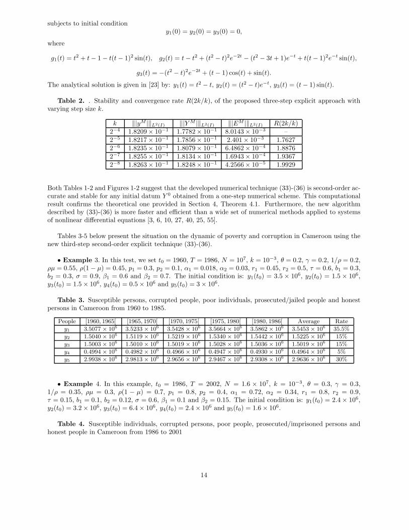
Table 2. . Stability and convergence rate R(2k/k), of the proposed three-step explicit approach withvarying step size k.

k ‖|yM |‖L2(I) ‖|YM |‖L2(I) ‖|EM |‖L2(I) R(2k/k)2−4 1.8209× 10−1 1.7782× 10−1 8.0143× 10−3 –2−5 1.8217× 10−1 1.7856× 10−1 2.401× 10−3 1.76272−6 1.8235× 10−1 1.8079× 10−1 6.4862× 10−4 1.88762−7 1.8255× 10−1 1.8134× 10−1 1.6943× 10−4 1.93672−8 1.8263× 10−1 1.8248× 10−1 4.2566× 10−5 1.9929

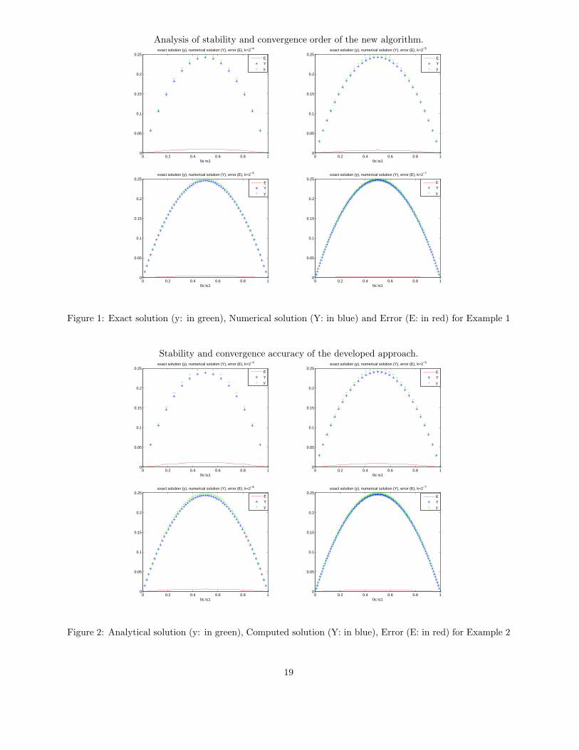
Both Tables 1-2 and Figures 1-2 suggest that the developed numerical technique (33)-(36) is second-order ac-curate and stable for any initial datum Y 0 obtained from a one-step numerical scheme. This computationalresult confirms the theoretical one provided in Section 4, Theorem 4.1. Furthermore, the new algorithmdescribed by (33)-(36) is more faster and efficient than a wide set of numerical methods applied to systemsof nonlinear differential equations [3, 6, 10, 27, 40, 25, 55].

Tables 3-5 below present the situation on the dynamic of poverty and corruption in Cameroon using thenew third-step second-order explicit technique (33)-(36).

• Example 3. In this test, we set t0 = 1960, T = 1986, N = 107, k = 10−3, θ = 0.2, γ = 0.2, 1/ρ = 0.2,ρµ = 0.55, ρ(1− µ) = 0.45, p1 = 0.3, p2 = 0.1, α1 = 0.018, α2 = 0.03, r1 = 0.45, r2 = 0.5, τ = 0.6, b1 = 0.3,b2 = 0.3, σ = 0.9, β1 = 0.6 and β2 = 0.7. The initial condition is: y1(t0) = 3.5 × 106, y2(t0) = 1.5 × 106,y3(t0) = 1.5× 106, y4(t0) = 0.5× 106 and y5(t0) = 3× 106.

Table 3. Susceptible persons, corrupted people, poor individuals, prosecuted/jailed people and honestpersons in Cameroon from 1960 to 1985.

People [1960, 1965[ [1965, 1970[ [1970, 1975[ [1975, 1980[ [1980, 1986[ Average Rate

y1 3.5077 × 106 3.5233 × 106 3.5428 × 106 3.5664 × 106 3.5862 × 106 3.5453 × 106 35.5%

y2 1.5040 × 106 1.5119 × 106 1.5219 × 106 1.5340 × 106 1.5442 × 106 1.5225 × 106 15%

y3 1.5003 × 106 1.5010 × 106 1.5019 × 106 1.5028 × 106 1.5036 × 106 1.5019 × 106 15%

y4 0.4994 × 106 0.4982 × 106 0.4966 × 106 0.4947 × 106 0.4930 × 106 0.4964 × 106 5%

y5 2.9938 × 106 2.9813 × 106 2.9656 × 106 2.9467 × 106 2.9308 × 106 2.9636 × 106 30%

• Example 4. In this example, t0 = 1986, T = 2002, N = 1.6 × 107, k = 10−3, θ = 0.3, γ = 0.3,1/ρ = 0.35, ρµ = 0.3, ρ(1 − µ) = 0.7, p1 = 0.8, p2 = 0.4, α1 = 0.72, α2 = 0.34, r1 = 0.8, r2 = 0.9,τ = 0.15, b1 = 0.1, b2 = 0.12, σ = 0.6, β1 = 0.1 and β2 = 0.15. The initial condition is: y1(t0) = 2.4× 106,y2(t0) = 3.2× 106, y3(t0) = 6.4× 106, y4(t0) = 2.4× 106 and y5(t0) = 1.6× 106.

Table 4. Susceptible individuals, corrupted persons, poor people, prosecuted/imprisoned persons andhonest people in Cameroon from 1986 to 2001

14

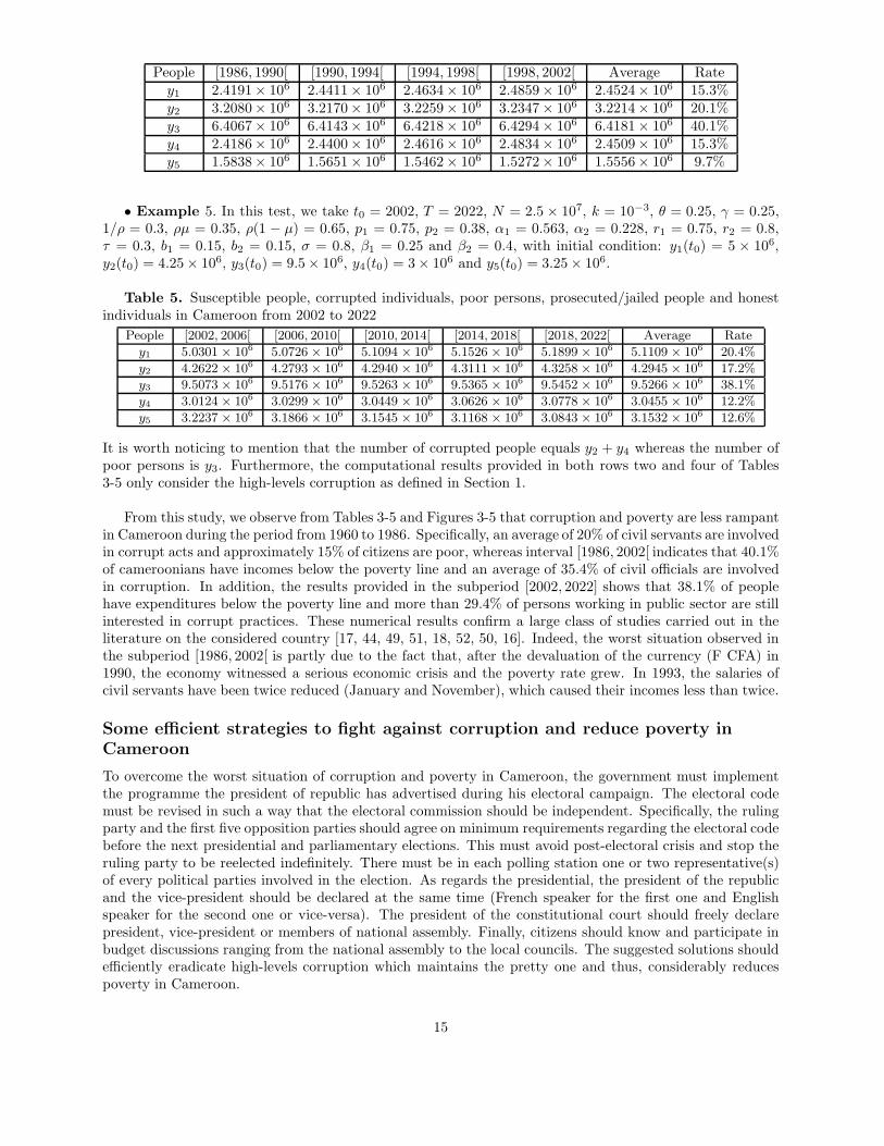
People [1986, 1990[ [1990, 1994[ [1994, 1998[ [1998, 2002[ Average Ratey1 2.4191× 106 2.4411× 106 2.4634× 106 2.4859× 106 2.4524× 106 15.3%y2 3.2080× 106 3.2170× 106 3.2259× 106 3.2347× 106 3.2214× 106 20.1%y3 6.4067× 106 6.4143× 106 6.4218× 106 6.4294× 106 6.4181× 106 40.1%y4 2.4186× 106 2.4400× 106 2.4616× 106 2.4834× 106 2.4509× 106 15.3%y5 1.5838× 106 1.5651× 106 1.5462× 106 1.5272× 106 1.5556× 106 9.7%

• Example 5. In this test, we take t0 = 2002, T = 2022, N = 2.5 × 107, k = 10−3, θ = 0.25, γ = 0.25,1/ρ = 0.3, ρµ = 0.35, ρ(1 − µ) = 0.65, p1 = 0.75, p2 = 0.38, α1 = 0.563, α2 = 0.228, r1 = 0.75, r2 = 0.8,τ = 0.3, b1 = 0.15, b2 = 0.15, σ = 0.8, β1 = 0.25 and β2 = 0.4, with initial condition: y1(t0) = 5 × 106,y2(t0) = 4.25× 106, y3(t0) = 9.5× 106, y4(t0) = 3× 106 and y5(t0) = 3.25× 106.

Table 5. Susceptible people, corrupted individuals, poor persons, prosecuted/jailed people and honestindividuals in Cameroon from 2002 to 2022

People [2002, 2006[ [2006, 2010[ [2010, 2014[ [2014, 2018[ [2018, 2022[ Average Rate

y1 5.0301 × 106 5.0726 × 106 5.1094 × 106 5.1526 × 106 5.1899 × 106 5.1109 × 106 20.4%

y2 4.2622 × 106 4.2793 × 106 4.2940 × 106 4.3111 × 106 4.3258 × 106 4.2945 × 106 17.2%

y3 9.5073 × 106 9.5176 × 106 9.5263 × 106 9.5365 × 106 9.5452 × 106 9.5266 × 106 38.1%

y4 3.0124 × 106 3.0299 × 106 3.0449 × 106 3.0626 × 106 3.0778 × 106 3.0455 × 106 12.2%

y5 3.2237 × 106 3.1866 × 106 3.1545 × 106 3.1168 × 106 3.0843 × 106 3.1532 × 106 12.6%

It is worth noticing to mention that the number of corrupted people equals y2 + y4 whereas the number ofpoor persons is y3. Furthermore, the computational results provided in both rows two and four of Tables3-5 only consider the high-levels corruption as defined in Section 1.

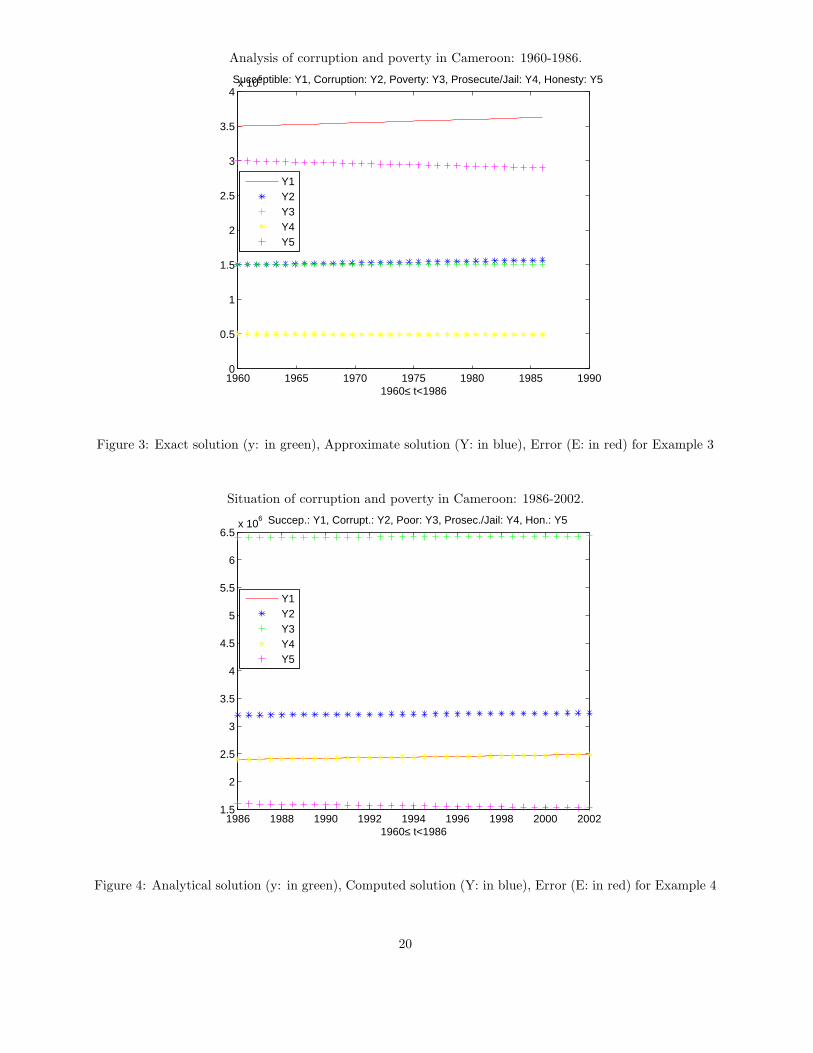
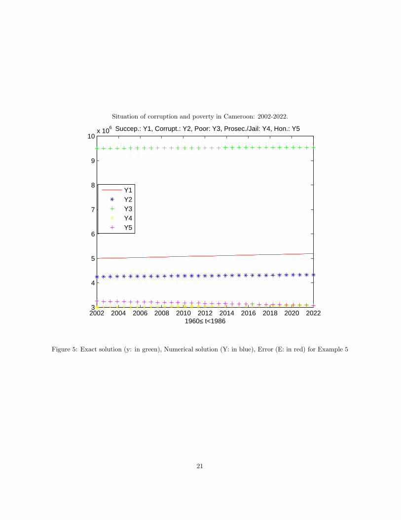
From this study, we observe from Tables 3-5 and Figures 3-5 that corruption and poverty are less rampantin Cameroon during the period from 1960 to 1986. Specifically, an average of 20% of civil servants are involvedin corrupt acts and approximately 15% of citizens are poor, whereas interval [1986, 2002[ indicates that 40.1%of cameroonians have incomes below the poverty line and an average of 35.4% of civil officials are involvedin corruption. In addition, the results provided in the subperiod [2002, 2022] shows that 38.1% of peoplehave expenditures below the poverty line and more than 29.4% of persons working in public sector are stillinterested in corrupt practices. These numerical results confirm a large class of studies carried out in theliterature on the considered country [17, 44, 49, 51, 18, 52, 50, 16]. Indeed, the worst situation observed inthe subperiod [1986, 2002[ is partly due to the fact that, after the devaluation of the currency (F CFA) in1990, the economy witnessed a serious economic crisis and the poverty rate grew. In 1993, the salaries ofcivil servants have been twice reduced (January and November), which caused their incomes less than twice.

Some efficient strategies to fight against corruption and reduce poverty in

Cameroon

To overcome the worst situation of corruption and poverty in Cameroon, the government must implementthe programme the president of republic has advertised during his electoral campaign. The electoral codemust be revised in such a way that the electoral commission should be independent. Specifically, the rulingparty and the first five opposition parties should agree on minimum requirements regarding the electoral codebefore the next presidential and parliamentary elections. This must avoid post-electoral crisis and stop theruling party to be reelected indefinitely. There must be in each polling station one or two representative(s)of every political parties involved in the election. As regards the presidential, the president of the republicand the vice-president should be declared at the same time (French speaker for the first one and Englishspeaker for the second one or vice-versa). The president of the constitutional court should freely declarepresident, vice-president or members of national assembly. Finally, citizens should know and participate inbudget discussions ranging from the national assembly to the local councils. The suggested solutions shouldefficiently eradicate high-levels corruption which maintains the pretty one and thus, considerably reducespoverty in Cameroon.

15

6 General conclusion and future works

In this paper, we have developed a third-step second-order explicit numerical approach in a computed solu-tion of a mathematical model on the dynamic of corruption and poverty (1)-(5), subjects to initial condition(6). The particular case on the dynamic of corruption and poverty in Cameroon has been discussed in theSection 5 (Numerical experiments). The theory has suggested that the proposed numerical technique issecond-order convergent and stable for any value of the initial datum (Theorem 4.1). This result is con-firmed by some numerical examples (see, Tables 1-2 and Figures 1-2). Furthermore, the study indicatesthat the new algorithm is fast and more efficient than a broad range of numerical schemes largely studiedin the literature for solving such systems of nonlinear differential equations [6, 10, 27, 40, 3, 55, 25]. Fi-nally, the developed numerical method is used to investigating and predicting the dynamic of corruptionand poverty in Cameroon. The results provided by Tables 3-5 and Figures 3-5 confirm those discussed in[21, 5, 52, 49, 50, 51]. Our future works will consider the development of a third-step third-order explicitmethod to assessing the dynamic of the poverty with effect of alcohol taking into account the particular caseof Cameroon.

Acknowledgment. This work has been partially supported by the Deanship of Scientific Research ofImam Mohammad Ibn Saud Islamic University (IMSIU) under the Grant No. 331203.

References

[1] Afrique L. ”Cameroun: Quelle strategie de lutte contre la corruption au sein de l’administrationpublique?”, (2011).

[2] B. Ames, W. Brown, S. Devarajan, A. Izquierdo. ”Poverty reduction strategy sourcebook”, chap 12,Macroeconomic issues, World Bank, Washington D.C, (2001).

[3] M. Arellano, S. Bond. ”Some tests of specification for panel data: Monte Carlo evidence and an appli-cation to employment equations”, Review of Economic Studies, 97 : 58-277 (1991).

[4] S. Athithan, M. Ghosh. ”Impact of case detection and treatment on the spread of hiv/aids: a mathe-matical study”, Malyasia J. Math. Sci., 12 (2018), 323-347.

[5] E. E. Bechem. ”Corruption in Cameroon: public perception on the role and effectiveness of the differentanti-corruption agencies”, Review of Public Administration and management, (2018).

[6] F. Brauer, C. Castillo-Chavez. ”Mathematical models in population biology and epidemiology”, in Textin Applied Mathematics, Springer, (2001).

[7] Cameroon Tribune. ”Cameroon tribune Journal”, Yaounde, (1998).

[8] CONAC. ”Rapport sur l’etat de la lutte contre la corruption au Cameroun”, Yaounde, (2017).

[9] CONAC. ”Cameroon’s 2018 anti-corruption status repport”, Yaounde, (2018).

[10] R. Codina, J. Principe, C. Munoz, J. Baiges. ”Numerical modeling of chlorine concentration in waterstorage tanks”, Int. J. Numer. Meth. Fluids, 79 (2015), 84-107.

[11] L. Cord. ”Poverty reduction strategy sourcebook”, chap 15, Rural poverty, Washington D.C, The WorldBank, (2001).

[12] G. Dahlquist. ”A special stability problem for linear multistep methods”, BIT 3, (1963), 27-43.

[13] G. Dahlquist. ”Cnvergence and stability in the numerical integration of ordinary differential equations”,Math. Scand. 4, (1956), 33-56.

[14] F. Y. Eguda, A. James, F. A. Oguntolu, D. Onah. ”Mathematical analysis of a model to investigate thedynamic of poverty and corruption”, Abacus (Mathematics Science Series), 44(1) (2019), 352-367.

16

[15] F. Y. Eguda, F. Oguntolu, T. T. Ashezua. ”Understanding the dynamic of corruption using mathemat-ical modeling approach”, Int. Innotive Science, 4(8) (2017).

[16] S. Fambon. ”A dynamic poverty profile for Cameroon”, AERC-UNECA Dissemination Conference onPoverty, Income Distribution and Labor Market in Sub-Saharan Africa: Phase II, (2006).

[17] S. Fambon, A. Mckay, J. P. Timnou, O. S. Kouakep, A. D. Dzossa, R. T. Ngoho. ”Slow progress ingrowth and poverty reduction in Cameroon”, Growth and Poverty in Sub-Saharan Africa, (2016).

[18] GERDDES-Cameroon. ”Corruption in Cameroon”, Yaounde: Friedrich-Ebert-Stiftung, (1999).

[19] N. Girishankar, L. Hammergren, M. Holmes, S. Knack, B. Levy, J. Litvack, N. Manning, R. Mes-sick, J. Rinne, H. Sutch. ”Poverty reduction strategy sourcebook”, chap 8, Governance, World Bank,Washington D.C, (2002).

[20] Global Financial Integraty. ”Illicit financial flows from Africa”, Hidden Resource for Development,(2015).

[21] N. Grimbald, N. D. Nchang, P. E. Mbuh. ”A critical assessment of the impact of corruption on theeconomic and social development of Cameroon”, Int. J. Innovative Research & Advanced Studies, 7(2),(2020).

[22] P. Henrici. ”Discrete variable methods in ordinary differential equations”, New York, John Wiley (1962).

[23] Y. Li, F. Geng, M. Cui. ”The analytical solution of a system of nonlinear differential equations”, Int.J. Math. Anal., 1(10) (2007), 451-462.

[24] Monde Afrique. ”Cameroun: L’impitoyable machine judiciaire de Paul Biya”, Cameroun: Friedrich-Ebert-Stiftung, (2015).

[25] S. Mushayabasa, C. Bhunu, C, Webb, M. Dhlamini. ”A mathematical model for assessing the impactof poverty on yaws eradications”, Appl. Math. Model., 36 (2012), 1653-(1667).

[26] V. Negin, Z. A. Rashid, H. Nikopour. ”The casual relationship between corruption and poverty: Apanal data analysis”, Munich (2010).

[27] E. Ngondiep. ”A robust numerical two-level second-order explicit approach to predicting the spread ofCovid-19 pandemic with undetected infectious cases”, J. Comput. Appl. Math., 403 (2022), 113852.

[28] E. Ngondiep. ”Unconditional stability over long time intervals of a two-level coupledMacCormack/Crank-Nicolson method for evolutionary mixed Stokes-Darcy model”, J. Comput. Appl.Math., 409(2022), 114148, Doi: 10.1016/j.cam.2022.114148.

[29] E. Ngondiep. ”Stability analysis of MacCormack rapid solver method for evolutionary Stokes-Darcyproblem”, J. Comput. Appl. Math. 345(2019), 269-285.

[30] E. Ngondiep. ”A two-level fourth-order approach for time-fractional convection-diffusion-reaction equa-tion with variable coefficients”, Commun. Nonlinear Sci. Numer. Simul., 111(2022), 106444, Doi:10.1016/j.cnsns.2022.106444.

[31] E. Ngondiep. ”A fourth-order two-level factored implicit scheme for solving two-dimensional unsteadytransport equation with time dependent dispersion coefficients”, Int. J. Comput. Meth. Engrg. Sci.Mech., 22(4) (2021), 253-264.

[32] E. Ngondiep. ”A novel three-level time-split MacCormack scheme for two-dimensional evolutionarylinear convection-diffusion-reaction equation with source term”, Int. J. Comput. Math., 98(1) (2021),47-74.

[33] E. Ngondiep. ”A novel three-level time-split approach for solving two-dimensional nonlinear unsteadyconvection-diffusion-reaction equation”, J. Math. Computer Sci., 26(3) (2022), 222-248.

17

[34] E. Ngondiep. ”Long time stability and convergence rate of MacCormack rapid solver method for non-stationary Stokes-Darcy problem”, Comput. Math. Appl., 75 (2018), 3663-3684.

[35] E. Ngondiep. ”An efficient three-level explicit time-split approach for solving 2D heat conduction equa-tions”, Appl. Math. Inf. Sci., 14(6), (2020), 1075-1092.

[36] E. Ngondiep. ”Unconditional stability of a two-step fourth-order modified explicit Euler/Crank-Nicolsonapproach for solving time-variable fractional mobile-immobile advection-dispersion equation”, preprintavailable online from https://arxiv.org/abs/2205.05077, (2022), 28 pages.

[37] E. Ngondiep. ”An efficient three-level explicit time-split scheme for solving two-dimensional unsteadynonlinear coupled Burgers equations”, Int. J. Numer. Methods Fluids, 92(4) (2020), 266-284.

[38] E. Ngondiep. ”A robust three-level time-split MacCormack scheme for solving two-dimensional unsteadyconvection-diffusion equation”, J. Appl. Comput. Mech., 7(2) (2021), 559-577.

[39] E. Ngondiep. ”Long time unconditional stability of a two-level hybrid method for nonstationary incom-pressible Navier-Stokes equations”, J. Comput. Appl. Math., 345(2019), 501-514.

[40] E. Ngondiep. ”An efficient explicit approach for predicting the Covid-19 spreading with undetectedinfectious: The case of Cameroon”, preprint available online from http://arxiv.org/abs/2005.11279,(2020), 26 pages.

[41] E. Ngondiep. ”A two-level factored Crank-Nicolson method for two-dimensional nonstationaryadvection-diffusion equation with time dependent dispersion coefficients and source/sink term”, Adv.Appl. Math. Mech., 13(5) (2021), 1005-1026.

[42] E. Ngondiep, N. Kerdid, M. A. M. Abaoud, I. A. I. Aldayel. ”A three-level time-split MacCormackmethod for two-dimensional nonlinear reaction-diffusion equations”, Int. J. Numer. Meth. Fluids, 92(12)(2020), 1681-1706.

[43] H. K. Oduwole, S. L. Shehu. ”A mathematical model on the dynamic of poverty and prostitution inNigeria”, Math. Theory Model., 3(12) (2013), 74-79.

[44] OECD. ”Illicit financial flows: The economy of illicit trade in west Africa”, (2018).

[45] J. T. Okola. ”La decennie Biya au Cameroun”, Paris, l’Harmattan, (1996).

[46] Price Water House. ”Impact of corruption in Nigeria’s economy”, (2016).

[47] M. Ravallion. ”Poverty lines across the world”, The World Bank, (2010).

[48] U. A. M. Roshan, S. Besbris, M. friedson. ”Poverty and crime”, in the Oxford handbook of the socialscience of poverty, (2016).

[49] Transparency International. ”Corruption perception index (CPI)”, (1998) & (1999).

[50] Transparency International. ”Global corruption barometer 2013”, Cameroon, (2013).

[51] Transparency International. ”Cameroon: Overview of corruption and anti-corruption”, (2016).

[52] United Nation Development Programme. ”Cameroon: Human Development Indicators”, (2005).

[53] C. a. Van Rijckeghem. ”Bureaucratic corruption and the rate of temptation: Do wages in the civilservices affect corruption, and by how much?”, J. Development Economics, 65(2) (2001), 307-331.

[54] World Bank. ”The cancer of corruption. World bank global issues seminar series”, (2005).

[55] H. Zhao, Z. Feng, C. Castillo-Chavez. ”The dynamic of poverty and crime”, J. Shanghai Normal Uni-versity (Natural Sci. Math.), 43 (2014), 486-495.

18

Analysis of stability and convergence order of the new algorithm.

0 0.2 0.4 0.6 0.8 10

0.05

0.1

0.15

0.2

0.25

0≤ t≤1

exact solution (y), numerical solution (Y), error (E), k=2−4

EYy

0 0.2 0.4 0.6 0.8 10

0.05

0.1

0.15

0.2

0.25

0≤ t≤1

exact solution (y), numerical solution (Y), error (E), k=2−5

EYy

0 0.2 0.4 0.6 0.8 10

0.05

0.1

0.15

0.2

0.25

0≤ t≤1

exact solution (y), numerical solution (Y), error (E), k=2−6

EYy

0 0.2 0.4 0.6 0.8 10

0.05

0.1

0.15

0.2

0.25

0≤ t≤1

exact solution (y), numerical solution (Y), error (E), k=2−7

EYy

Figure 1: Exact solution (y: in green), Numerical solution (Y: in blue) and Error (E: in red) for Example 1

Stability and convergence accuracy of the developed approach.

0 0.2 0.4 0.6 0.8 10

0.05

0.1

0.15

0.2

0.25

0≤ t≤1

exact solution (y), numerical solution (Y), error (E), k=2−4

EYy

0 0.2 0.4 0.6 0.8 10

0.05

0.1

0.15

0.2

0.25

0≤ t≤1

exact solution (y), numerical solution (Y), error (E), k=2−5

EYy

0 0.2 0.4 0.6 0.8 10

0.05

0.1

0.15

0.2

0.25

0≤ t≤1

exact solution (y), numerical solution (Y), error (E), k=2−6

EYy

0 0.2 0.4 0.6 0.8 10

0.05

0.1

0.15

0.2

0.25

0≤ t≤1

exact solution (y), numerical solution (Y), error (E), k=2−7

EYy

Figure 2: Analytical solution (y: in green), Computed solution (Y: in blue), Error (E: in red) for Example 2

19

Analysis of corruption and poverty in Cameroon: 1960-1986.

1960 1965 1970 1975 1980 1985 19900

0.5

1

1.5

2

2.5

3

3.5

4x 10

6

1960≤ t<1986

Succeptible: Y1, Corruption: Y2, Poverty: Y3, Prosecute/Jail: Y4, Honesty: Y5

Y1Y2Y3Y4Y5

Figure 3: Exact solution (y: in green), Approximate solution (Y: in blue), Error (E: in red) for Example 3

Situation of corruption and poverty in Cameroon: 1986-2002.

1986 1988 1990 1992 1994 1996 1998 2000 20021.5

2

2.5

3

3.5

4

4.5

5

5.5

6

6.5x 10

6

1960≤ t<1986

Succep.: Y1, Corrupt.: Y2, Poor: Y3, Prosec./Jail: Y4, Hon.: Y5

Y1Y2Y3Y4Y5

Figure 4: Analytical solution (y: in green), Computed solution (Y: in blue), Error (E: in red) for Example 4

20

Situation of corruption and poverty in Cameroon: 2002-2022.

2002 2004 2006 2008 2010 2012 2014 2016 2018 2020 20223

4

5

6

7

8

9

10x 10

6

1960≤ t<1986

Succep.: Y1, Corrupt.: Y2, Poor: Y3, Prosec./Jail: Y4, Hon.: Y5

Y1Y2Y3Y4Y5

Figure 5: Exact solution (y: in green), Numerical solution (Y: in blue), Error (E: in red) for Example 5

21