A fast Lagrangian heuristic for large-scale capacitated lot-size problems with restricted cost structures

KYB ERNET IK A — VO LUME 4 8 ( 2 0 1 2 ) , NUMBER 2 , PAGES 3 2 9 – 3 4 5

A FAST LAGRANGIAN HEURISTIC FOR LARGE-SCALECAPACITATED LOT-SIZE PROBLEMS WITHRESTRICTED COST STRUCTURES

Kjetil K. Haugen, Guillaume Lanquepin-Chesnais and Asmund Olstad

In this paper, we demonstrate the computational consequences of making a simple assump-tion on production cost structures in capacitated lot-size problems. Our results indicate thatour cost assumption of increased productivity over time has dramatic effects on the problemsizes which are solvable.

Our experiments indicate that problems with more than 1000 products in more than 1000time periods may be solved within reasonable time. The Lagrangian decomposition algorithmwe use does of course not guarantee optimality, but our results indicate surprisingly narrowgaps for such large-scale cases – in most cases significantly outperforming CPLEX.

We also demonstrate that general CLSP’s can benefit greatly from applying our proposedheuristic.

Keywords: heuristics, capacitated lot-sizing, restricted cost structures

Classification: 65K05, 90B30, 68W99

1. INTRODUCTION

The capacitated lot-size problem (CLSP) has drawn significant research attention sinceManne’s [16] original MILP formulation more than 50 years ago. Several review arti-cles [6, 13, 15] and [3] indicate the size, diversity and complexity of CLSP-research.

Karimi et al. [13] categorizes CLSP algorithmic research related to solution methodsin various categories. Of particular interest for this work is the subcategory of RelaxationHeuristics. According to Karimi et al. [13], such heuristics usually produce better qualitysolutions, are more general and allow extensions to different problems.

In spite of extensive research, the size of problems practically feasible are limited.By practically feasible, we mean problems that can be solved in reasonable time withinan acceptable deviation from optimum. As modern product variety may involve vastproduct counts, the reported sizes of problems practically feasible are still far from realworld cases.

However, some articles do report large-scale CLSP-like problems solved. Diabyet al. [5] report problem sizes of up to 5000 products in 30 time periods. Compara-ble problem sizes are reported by Haugen et al. [11]. Common for these applications arereformulations of the CLSP introducing added problem flexibility. Diaby et al. [5] allow

330 K. K. HAUGEN, G. LANQUEPIN-CHESNAIS AND A. OLSTAD

overtime usage, while Haugen et al. [11, 10] introduce demand-affecting prices. Hence,both these two approaches solve other problems than CLSP.

Our aim in this article, is to investigate a different angle of attack in order to achievesolution speed for problem sizes closer to real world cases without relaxing the originalCLSP formulation. Still, certain research facts must be considered; the strong NP-hardness of CLSP [2, 4]. Consequently, we need to apply some tricks.

In section 2, we introduce our CLSP formulation while section 3 discusses our al-gorithmic set-up as well as our cost assumptions. Section 4 contains our numericalexperiments, while the article concludes and suggests possible further research in sec-tion 5.

2. OUR CLSP FORMULATION

At this point, a mathematical formulation of CLSP is appropriate. The Single-level (bigbucket) CLSP may be formulated as:

Minimise Z =T∑

t=1

J∑j=1

[sjtδjt + hjtIjt + cjtxjt] (1)

Subject to∑J

j=1 ajtxjt ≤ Rt ∀ t (2)xjt + Ij,t−1 − Ijt = djt ∀ jt (3)

0 ≤ xjt ≤ Mjtδjt ∀ jt (4)Ijt ≥ 0, ∀ jt (5)

δjt ∈ {0, 1} ∀ jt (6)j ∈ {1, 2, . . . , J} (7)t ∈ {1, 2, . . . , T} (8)

with decision variables:

xjt : the amount of item j produced in period t

Ijt : amount of item j held in inventory between periods t, t + 1δjt : 1 if item j is produced in period t ; 0 otherwise

and parameters:

T : number of time periodsJ : number of items

sjt : setup cost for itemj in period t

hjt : storage cost for item j between periods t, t + 1cjt : unit production cost for item j in period t

A fast Lagrangian heuristic for large-scale CLSP problems 331

ajt : consumption of capacitated resource by item j in period t

Rt : amount of capacity resource available in period t

djt : given future demand for product j in time period t

Mjt : this is the smallest possible “Big M” needed to take

care of binary logic for product j in period t, Mjt =∑T

s=tdjs,

I0 : Initial inventory > 0.

The objective (1) contains total costs (set-up, storage and production). Constraints (2)are the capacity constraints and (3) inventory balancing, while (4), with the integral-ity requirement (6), enforces set-up when production is positive. Non-negativity con-straints (5) are reasonable. (7) and (8) define ranges for indices.

3. OUR ALGORITHMIC SET-UP

3.1. Relaxation heuristics — Lagrangian relaxation

The trick mentioned in section 1 is related to assumptions on cost structures. If wecan make reasonable (read practically relevant) assumptions on cost structures, easingthe computational burden in certain sub problems, we can hope to achieve speed-upscompared to existing research.

In order to explain how and why our approach works, we need to explain the basicsof Lagrangian relaxation. As indicated in section 1, Relaxation Heuristics is a centraltechnique in CLSP-heuristic research. The technique works as follows: Firstly, the perperiod capacity constraint (2) is relaxed (added to the objective (1)). As a consequence,J decoupled sub problems – for instance solvable by the Wagner–Whitin algorithm [20]1

– emerges. By solving these problems, set-up structures for each product j is obtained,and the solution for the common problem will constitute a lower bound for the orig-inal problem. Secondly, this set-up structure is applied in order to fix correspondingbinary (set-up) variables resulting in an LP sub problem, producing an upper bound onthe solution of the original problem, which is solved to produce Lagrangian multipliers(shadow prices). We name the first problem set LB-problems, while the second problemset is named UB-problems2. These values are then fed back into the original relaxedproblem as new multipliers. Now, the basic Lagrangian relaxation loop is constructedand improved solutions are obtained running back and forth between the UB- and theLB-problems.

The above described algorithmic set-up was used by both Thizy and Wassenhove [18]and Trigeiro [19] in their trend-setting articles. Hence, our choice of relaxing the capacityconstraint (2) is in accordance with existing theory. This fact is also supported by Chenand Thizy [4] as well as research by Haugen et al. [10, 11].

The main difference between these approaches is perhaps related to Trigeiro’s useof Lagrangian multiplier smoothing techniques. A similar set-up (including smoothing)was used by Haugen et al. [10, 11].

1We apply a slightly modified version of the original algorithm as reported by Wagelmans et al. [21]2See appendices B and C for additional information on both formulation as well as solution strategies

for these sub problems.

332 K. K. HAUGEN, G. LANQUEPIN-CHESNAIS AND A. OLSTAD

3.2. Cost assumptions

The specialized cost assumptions we apply are needed in order to solve the UB-problemsmore efficient. We apply a technique recently proposed and demonstrated by Haugenet al. [9]. As the technique is well described in [9], we will just discuss it briefly. In orderto keep things simple, we investigate a single product case. The multi product case isdiscussed in detail in [9].

If all binary variables (δjt’s) in the CLSP-formulation (1) – (8) are fixed, the resultingLP may be formulated3:

Minimise Z =T∑

t=1

[htIt + ctxt] (9)

Subject to xt ≤ Rt ∀ t (10)xt + It−1 − It = dt ∀ t (11)

xt ≥ 0 ∀ t (12)It ≥ 0 ∀ t. (13)

If we start by assuming constant production costs (c1 = c2 = . . . cT = c), it isstraightforward to show (see Haugen et al. [9]) that the objective can be reformulatedto:

Minimise Z =T∑

t=1

htIt. (14)

Given this, it is obvious that the optimal solution to the LP must be the “Just-in-time” solution (x∗t = dt∀ t), given that this solution is feasible (i. e. not violating theconstraint (10)). If the capacity constraint is violated say in time period τ1, then we canarrive at an optimal solution by “shuffling”4 production from this time period τ1 to thenearest time period (τ2 < τ1) with spare capacity. Any other time period choice furtheraway, will increase total inventory costs. Furthermore, it is likewise clear that given thefollowing revised production cost assumption;

c1 ≥ c2 ≥ . . . ≥ cT (15)

the above argument is still valid.This argument is easily extended to the multi-item case – see Haugen et al. [9],

providing an extremely efficient specialized algorithm for the (LP) UB-problems.If our proposed algorithm for CLSP turns out to be successful, which later sections

indeed will reveal, the practical usability will rely on whether our added cost restrictionsfits reality. Our cost assumption (15) is limited to production costs. Production costsare market determined. As such, it would be very surprising if a certain producer wouldbe able to predict them.

3Note that T in equation (9) typically is different from T (T ≤ T ) in equation (1) due to fixation ofthe binary variables.

4We name this algorithm the “ bulldozer” algorithm for further reference. The choice of name is dueto it’s similarity to a bulldozer clearing snow by shuffling it to the closest possible storage location.

A fast Lagrangian heuristic for large-scale CLSP problems 333

Production costs contain (primarily) wages and technology. Both factors are hard topredict. If some producer actually could predict changes from a given average value, itmight be opportune to ask if the producer perhaps should engage in finance market spec-ulative activities instead of running CLSP-problems to organize local production. In anycase, one would typically observe decreasing production costs if empirical observationsare performed. One could think about most modern products who at the introductionphase typically will have high per unit production costs. Even if wages, and most otherproduction inputs have increasing costs, per unit product costs normally decrease dueto productivity increase over a product’s life-cycle. Let us try to sum up: If productioncosts are to change, they should (logically) change in a decreasing way, covered by ourassumption (15). Alternatively, in the short run, it is hard to see producers being ableto beat the market by forecasting labour and technology better.

3.3. An added approximation

As indicated by several authors (see e. g. [8, 12] or [11]), solving sub-problems to op-timality in Lagrangian decomposition may prove inefficient. The main point in thesetechniques is to achieve direction as opposed to exactness. As such, we could try toimprove speed by investigating certain approximations for our proposed sub problemsolvers. The “bulldozer” algorithm discussed above is simply so fast, that added ap-proximations seems unlikely to induce improvements.

3.4. Solving the LB-problem

The LB-problems however, may be interesting to investigate further in approximationsor new heuristics. Even though the DP-based WW-algorithm [20, 21], is extremelyefficient, it provides much of the computational burden in our proposed algorithmic set-up. As a consequence, we propose (in many ways similar to Kirca and Kokten [14]) toapply a very simple EOQ5-approximation [7] as an alternative to the exact6 WW-solver.A more thorough description of this approximation is left for appendix A.

Our algorithmic set-up is summarized in Figure 1.The LB-problems are either solved by a “normal” WW-algorithm [20, 21] or by

our EOQ-approximation described in appendix A. The UB-problems are solved by the“Bulldozer”-algorithm described in subsection 3.2.

A final point should be mentioned. In order to ease the problem of achieving feasibilityin the “Bulldozer”-stage, we have allowed a dynamic Lagrangian multiplier smoothingprocedure. That is, we open up for using different smoothing parameters at differentiteration steps in our Lagrangian relaxation heuristic.

4. NUMERICAL EXPERIMENTS

4.1. Computational set-up

All our numerical experiments are performed on a HP z400 equipped with the Intel XeonW3520 processor and 8GB DDR3 RAM. The software platform contains gcc: 4.4.5,

5Economic Order Quantity6Exactness means to optimality here.

334 K. K. HAUGEN, G. LANQUEPIN-CHESNAIS AND A. OLSTAD

Fig. 1. The algorithmic set-up.

Python: 2.6.6, Pyrex: 0.9.8.5, Cplex: 12.2.0.0 (from python wrapper) and Cython: 0.14(only used for the tests in appendix A). The experiments are mainly done in UbuntuLinux 10.10 64bits Maverick, but certain operations were performed in Windows XP32bits SP3 (running inside virtualbox 4.0.0).

All additional information on cases, run-times, graphics and so forth are (of course)obtainable from the authors upon request.

4.2. Trigeiro cases

We start out by examining our heuristics performance on some standard problems fromliterature, originally defined by Trigeiro et al [19] and collected by Wolsey and Bel-vaux [1]. We pick the six standard cases; tr6-15, tr6-30, tr12-15, tr12-30, tr24-15and tr24-30. The numbers in the case-names refers to the number of products and timeperiods respectively7.

Table 1 sums up our results. (All cases are run with “WW” as the LB-problem-solver.)

Case J T Zh ZCPLEX CPU(s) Z∗ CPU∗(s)tr6-15 6 15 39896 52800 0.0125 37092 0.1213tr6-30 6 30 69899 86600 0.0499 60835 0.6587tr12-15 12 15 78563 81640 0.6587 70922 0.8751tr12-30 12 30 160746 189249 0.6039 129788 12.0592tr24-15 24 15 143418 192000 0.0763 135970 0.9582tr24-30 24 30 310977 434600 0.1433 287425 3.8429

Tab. 1. Results for the Trigeiro cases.

In Table 1, the three first columns denote case name, number of products (J) andnumber of time periods (T ) respectively. The columns labelled Zh and ZCPLEX contains

7That is, the tr6-15-case contains 6 products in 15 time periods.

A fast Lagrangian heuristic for large-scale CLSP problems 335

CLSP objective function values for our heuristic and CPLEX. These objective functionvalues are obtained by running our heuristic and CPLEX (pairwise) for the same amountof CPU-time (in seconds) given in the column labelled CPU(s). The final columns (Z∗)and (CPU∗(s)) contain optimal objective function values found by CPLEX as well ascorresponding CPU-times.

We observe immediately, that our heuristic (by this measurement method) outper-forms CPLEX for all cases as Zh � ZCPLEX.

Table 2, calculated based on the information in Table 1 provides a clearer image.

Case∣∣∣Zh−ZCPLEX

Zh

∣∣∣ · 100 %∣∣∣Z∗−Zh

Z∗

∣∣∣ · 100 %∣∣∣Z∗−ZCPLEX

Z∗

∣∣∣ · 100 %

tr6-15 32.34% 7.56% 42.35%tr6-30 23.89% 14.90% 42.35%tr12-15 3.92% 10.77% 15.11%tr12-30 17.73% 23.85% 45.81%tr24-15 33.87% 5.48% 41.21%tr24-30 39.75% 8.19% 51.20%Average (%) 25.25% 11.79% 39.67 %

Tab. 2. Deviations (%) for the Trigeiro cases.

The first result-column (∣∣∣Zh−ZCPLEX

Zh

∣∣∣ · 100 %) in Table 2 shows that our heuristic onaverage produces around 25% better solutions than CPLEX for the same amount ofexecution time. Furthermore, our heuristic is on average slightly below 12 % from theoptimal value (

∣∣∣Z∗−Zh

Z∗

∣∣∣ · 100 %), while CPLEX is around 40% away from optimality

(∣∣∣Z∗−ZCPLEX

Z∗

∣∣∣ · 100 %).The above cases, originally considered hard, are of course easily solved on today’s

hard- and software. In fact, CPLEX proves optimality for the Trigeiro cases rangingfrom 0.12 CPU-seconds for the tr6-15 case up to 12.06 CPU-seconds for the tr12-30case. As such, our algorithm does not introduce any “revolution” for these cases, apartform the obvious fact that it produces good quality solutions significantly faster thanCPLEX.

4.3. Some medium sized examples and behaviour compared to CPLEX

In order to test our heuristic more seriously, we have made our own cases. These casesrange from relatively small cases 10 × 10 (10 products in 10 time) periods up to quitelarge cases of 200 × 10, 10 × 200 and 50 × 50. The terminology Y × Z will be used insubsequent sections where Y is number of products and Z is number of time periods.

For all costs, holding costs (hjt) are always set to 1 and production costs (cjt) to20. The set-up costs (sjt) are randomly picked within the set [100, 200, 300, 400, 500]but kept constant after the pick. Demand is a matrix (product × period) of pseudo-Gaussian (rounded to get integer and positive numbers). The capacity constraint (Rt)at time period t is the multiplication of a Gaussian (mean=ratio, var=0.01) generatednumber and the sum of the demand for the period.

336 K. K. HAUGEN, G. LANQUEPIN-CHESNAIS AND A. OLSTAD

All data are written in two formats; AMPL and MPS, the AMPL format is read byour heuristic and the MPS-file by CPLEX.

Before we move into some computationally more interesting cases, we present a simpleanalysis of our algorithm’s behaviour related to problem tightness. Figure 2 shows ourresults.

●

●

1.2 1.5 2

05

1015

2025

3035

Average ratio (constraint/demand)

GA

P (

%)

Fig. 2. Heuristic behaviour as a function of problem tightness.

The boxplot8 in Figure 2 is constructed by running a total of 35 cases ranging from10 × 10 by 5 × 20 up to 50 × 10. We have defined three different problem classes basedon problem tightness visualized on the Average ratio-axis in the box plot. Each boxholds a different tightness computed as J ·

PTt=1 RtPJ

j=1PT

t=1 djt. Consequently, the family of

cases representing the left-most box (the value 1.2) are really tight problems, while theright-most box of 2.0 represents more loose problems.

As can be readily observed from Figure 2, our heuristic (not very surprisingly) behavesbetter for less tight problems. For instance, the average GAP(%) from the optimal valueis found slightly above 25 %9 for the tightest family, while the relatively loose family withan Average ratio of 2 on average has only around 5% deviation from the optimal value.

This observation does not necessarily indicate that our heuristic performs badly ontight cases, but that it performs significantly better on less tight cases. The Trigeirocases in Tables 1, 2 are in fact quite tight with an Average ratio of 1.32.

8We use standard boxplots, visualising probability distributions efficiently. The height of a box givesvery visible information on variance of the distribution. A narrow box indicates small variance.

9The solid black line in the leftmost box.

A fast Lagrangian heuristic for large-scale CLSP problems 337

The main body of medium sized problems in our analysis is reported in Figures 3, 4

and 5. These cases10, substantially bigger, contain cases within 10 × 200, 200 × 10 and50 × 50.

Fig. 3. Objective function value as a function of CPU-time for

10 × 200 cases.

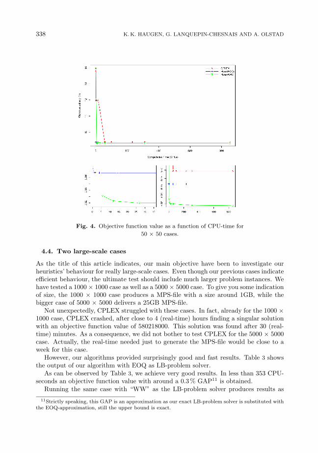
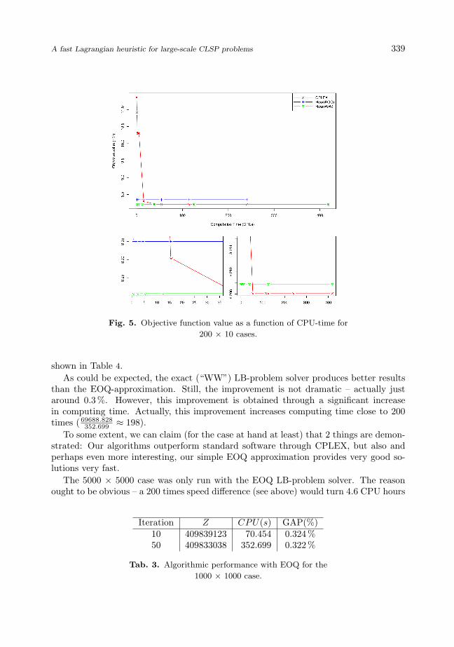
All Figures 3, 4 and 5 contain CLSP objective function value as a function of CPU-time. Each figure contains 3 different solution instances; CPLEX, and our algorithmeither with “WW” or EQO as LB-problem solvers. Furthermore, the two panes at thebottom are zoomed parts of the chart on top.

A closer inspection of Figures 3 and 4 reveals a similar type of pattern. The EOQversion (the blue curve) finds a relatively good solution extremely fast. Slightly slower,the “WW” version (the green curve) finds a better solution, while CPLEX (the redcurve) struggles and do not show solutions better than hour heuristic within the observedinterval of computational time.

However, the Branch and Bound Algorithm of CPLEX should of course in the endproduce the optimal value, which is not guaranteed by our heuristic. Indeed, this isobserved in Figure 5. Still, our heuristics produce relatively good solutions very fastcompared to CPLEX.

1015 generated cases in each category.

338 K. K. HAUGEN, G. LANQUEPIN-CHESNAIS AND A. OLSTAD

Fig. 4. Objective function value as a function of CPU-time for

50 × 50 cases.

4.4. Two large-scale cases

As the title of this article indicates, our main objective have been to investigate ourheuristics’ behaviour for really large-scale cases. Even though our previous cases indicateefficient behaviour, the ultimate test should include much larger problem instances. Wehave tested a 1000 × 1000 case as well as a 5000 × 5000 case. To give you some indicationof size, the 1000 × 1000 case produces a MPS-file with a size around 1GB, while thebigger case of 5000 × 5000 delivers a 25GB MPS-file.

Not unexpectedly, CPLEX struggled with these cases. In fact, already for the 1000 ×1000 case, CPLEX crashed, after close to 4 (real-time) hours finding a singular solutionwith an objective function value of 580218000. This solution was found after 30 (real-time) minutes. As a consequence, we did not bother to test CPLEX for the 5000 × 5000case. Actually, the real-time needed just to generate the MPS-file would be close to aweek for this case.

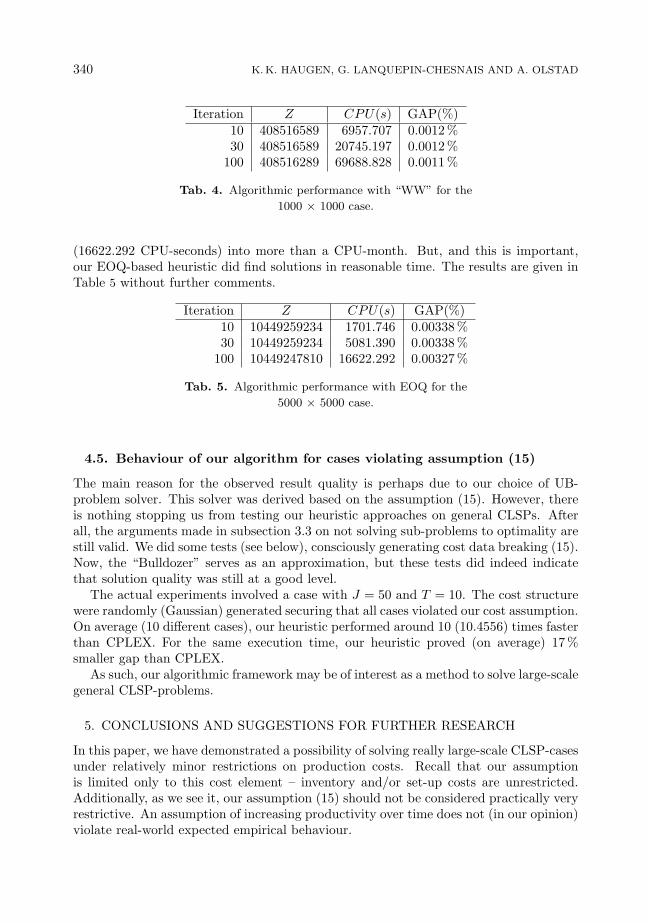
However, our algorithms provided surprisingly good and fast results. Table 3 showsthe output of our algorithm with EOQ as LB-problem solver.

As can be observed by Table 3, we achieve very good results. In less than 353 CPU-seconds an objective function value with around a 0.3% GAP11 is obtained.

Running the same case with “WW” as the LB-problem solver produces results as

11Strictly speaking, this GAP is an approximation as our exact LB-problem solver is substituted withthe EOQ-approximation, still the upper bound is exact.

A fast Lagrangian heuristic for large-scale CLSP problems 339

Fig. 5. Objective function value as a function of CPU-time for

200 × 10 cases.

shown in Table 4.As could be expected, the exact (“WW”) LB-problem solver produces better results

than the EOQ-approximation. Still, the improvement is not dramatic – actually justaround 0.3%. However, this improvement is obtained through a significant increasein computing time. Actually, this improvement increases computing time close to 200times ( 69688.828

352.699 ≈ 198).To some extent, we can claim (for the case at hand at least) that 2 things are demon-

strated: Our algorithms outperform standard software through CPLEX, but also andperhaps even more interesting, our simple EOQ approximation provides very good so-lutions very fast.

The 5000 × 5000 case was only run with the EOQ LB-problem solver. The reasonought to be obvious – a 200 times speed difference (see above) would turn 4.6 CPU hours

Iteration Z CPU(s) GAP(%)10 409839123 70.454 0.324%50 409833038 352.699 0.322%

Tab. 3. Algorithmic performance with EOQ for the

1000 × 1000 case.

340 K. K. HAUGEN, G. LANQUEPIN-CHESNAIS AND A. OLSTAD

Iteration Z CPU(s) GAP(%)10 408516589 6957.707 0.0012 %30 408516589 20745.197 0.0012 %

100 408516289 69688.828 0.0011 %

Tab. 4. Algorithmic performance with “WW” for the

1000 × 1000 case.

(16622.292 CPU-seconds) into more than a CPU-month. But, and this is important,our EOQ-based heuristic did find solutions in reasonable time. The results are given inTable 5 without further comments.

Iteration Z CPU(s) GAP(%)10 10449259234 1701.746 0.00338 %30 10449259234 5081.390 0.00338 %

100 10449247810 16622.292 0.00327 %

Tab. 5. Algorithmic performance with EOQ for the

5000 × 5000 case.

4.5. Behaviour of our algorithm for cases violating assumption (15)

The main reason for the observed result quality is perhaps due to our choice of UB-problem solver. This solver was derived based on the assumption (15). However, thereis nothing stopping us from testing our heuristic approaches on general CLSPs. Afterall, the arguments made in subsection 3.3 on not solving sub-problems to optimality arestill valid. We did some tests (see below), consciously generating cost data breaking (15).Now, the “Bulldozer” serves as an approximation, but these tests did indeed indicatethat solution quality was still at a good level.

The actual experiments involved a case with J = 50 and T = 10. The cost structurewere randomly (Gaussian) generated securing that all cases violated our cost assumption.On average (10 different cases), our heuristic performed around 10 (10.4556) times fasterthan CPLEX. For the same execution time, our heuristic proved (on average) 17%smaller gap than CPLEX.

As such, our algorithmic framework may be of interest as a method to solve large-scalegeneral CLSP-problems.

5. CONCLUSIONS AND SUGGESTIONS FOR FURTHER RESEARCH

In this paper, we have demonstrated a possibility of solving really large-scale CLSP-casesunder relatively minor restrictions on production costs. Recall that our assumptionis limited only to this cost element – inventory and/or set-up costs are unrestricted.Additionally, as we see it, our assumption (15) should not be considered practically veryrestrictive. An assumption of increasing productivity over time does not (in our opinion)violate real-world expected empirical behaviour.

A fast Lagrangian heuristic for large-scale CLSP problems 341

As opposed to other research reporting really large-scale cases, we do not reformulatethe original CLSP. There may of course be very good reasons for doing so (see e. g.Haugen [10]), but we still feel that the original CLSP are of practical relevance.

There are several options to improve our algorithmic choice. For instance, choosingeither “WW” or EOQ as a sub-problem solver for the LB-problems could be extendedto applying a combination. An interesting strategy to investigate could be to applyEOQ initially, to acquire a relatively good solution fast, and then continue with “WW”in order to improve on this solution. We have not tested this option, though obviouslyfeasible. Furthermore, a closer look into the possibility of more serious applications ofdynamic smoothing may prove interesting. A classical feature of the type of heuristicwe have applied is cycling. Previous research (see for instance [10] or [11]) indicatesalgorithmic sensitivity with regards to the either static or dynamic choices of smoothingparameter(s). An algorithmic scheme with the possibility of changing these parametersdynamically seems an interesting candidate to investigate further.

Finally, it seems fair to stress that we merely have demonstrated the potential ofour algorithms in solving really large-scale CLSPs. Surely, it is necessary to formulatea much wider set of problem instances for testing in order to get a better feeling forbehaviour of such cases. Still, we find our results both interesting as well as surprisingwhen it comes to observed solution quality and execution speed.

A. A SHORT DESCRIPTION OF OUR EOQ APPROXIMATION

It is of course well know from classical literature (see for instance the classical text-bookby Nahmias [17]) that the EOQ model may serve as an approximation in solving dynamiclot-size models. Such an approximation will improve if demand variability is moderate,and Wagner and Whitin themselves actually demonstrate the limiting behaviour of theirWW-algorithm in the original paper [20].

Our approach can be described as follows:

1) Compute EOQj for all products j ∈ {1, . . . , J}.

2) Make necessary adjustments on EOQj computed in 1) in order to spawn produc-tion costs.

3) ∀ j ∈ {1, . . . , J} find set-up structures.

Point 1) above is straightforward. We compute average demand per product dj =1T

∑Tt=1 djt and compute EOQj =

√2dj sj

hj, where sj and hj are average set-up and

inventory costs respectively.As our model contains production costs, point 2) indicates that we must adjust the

above calculated values for EOQj by some factor reflecting this. Some trial and errorlead to the adjustment factors for EOQj of the form K

(cjt + ajtλ

kjt

), where K is some

norming constant (revealed through experiments), and λkjt is the Lagrangian multiplier

for product j in time period t at iteration step k.

Point 3) is then simply performed by picking the EOQ-values(EOQj =

√2dj sj

hj

)and looping through the given demand (over t) until aggregate demand is larger thanthe given EOQ-value. This time period makes the next set-up period.

342 K. K. HAUGEN, G. LANQUEPIN-CHESNAIS AND A. OLSTAD

Table 6 highlights the quality of a such an algorithm, as it produces results quality-wise comparable to the Silver and Meal (SM) and Part Period Balancing (PPB) heuris-tics; more than two times faster. SM approximates the original lot-size problem bylooking at average costs instead of total costs. EOQ looks at total costs, but alterna-tively approximates demand. PPB is a kind of intermediate approach between EOQand SM.

The data in Table 6 are computed for 20 randomly generated data sets (one productin 20 time periods) where all costs are constant. Demand is uniformly generated on theinterval [0, 20].

Min. 1st Qu. Median Mean 3rd Qu. Max. CPUsSM 0 0.74 3.4 3.8 5 13 0.43PPB 0 1.6 3.8 7 9.7 25 0.43EOQ 0.53 1.2 2 4.9 5.1 23 0.16

Tab. 6. Quantiles, mean and median of relative errors (%) and

Computation time (ms)-

B. DESCRIPTION OF LB-PROBLEMS

The LB-problems referred in subsection 3.1 may be formulated as:

Min Z =T∑

t=1

J∑j=1

[sjtδjt + hjtIjt + cjtxjt]

+T∑

t=1

λt

J∑j=1

ajtxjt −Rt

(16)

s.t. the constraints (3) to (8).

where all parameters and variables are defined in section 2. (16) can be reformulatedas:

Min Z =T∑

t=1

J∑j=1

[sjtδjt + hjtIjt + cjtxjt]−T∑

t=1

λtRt (17)

s.t. the constraints (3) to (8).

where cjt = cjt + λtajt. Now, for given values of λt, the final part of (17) is a constantan can be removed from the objective. As a consequence, the remaining problem isidentical to the original Wagner/Whitin [20] formulation.

The LB-problem is then solved either by a modern version of the original Wag-ner/Whitin Dynamic Programming algorithm [21] or by our EOQ-approximation de-scribed in appendix A.

A fast Lagrangian heuristic for large-scale CLSP problems 343

C. DESCRIPTION OF UB-PROBLEMS

In this appendix we formulate and show our proposed algorithmic choices for The LBproblems referred in subsection 3.1. These problems can be formulated (As LinearPrograms) by equations (18) – (22) where variables and parameters are the same asdefined in section 2 apart from T which is different from the original T . This differenceoccurs due to the problem structure where binary variables are fixed and T is hencesmaller than or equal to T .

Min Z =J∑

j=1

T∑t=1

[hjtIjt + cjtxjt] (18)

s.t.

I∑j=1

ajtxjt ≤ Rt ∀ t (19)

xjt + Ij,t−1 − Ijt = djt ∀ j, t (20)xjt ≥ 0 ∀ t (21)Ijt ≥ 0 ∀ t. (22)

An pseudo-code algorithm for the single item version of (18) – (22) is shown below:

0. LET x∗t = dt,∀ t

1. IF x∗t ≤ Rt,∀ t STOP (x∗t is optimal)

2. IF next period is T + 1 STOP

3. ELSE find next period, τ where x∗t > Rt and produce a total of x∗t −Rt

in previous periods τ−1, τ−2, . . . as close as possible to τ . (If impossible,problem is infeasible STOP)

4. SET x∗τ = Rτ and update x∗τ−1, x∗τ−2, . . . correspondingly

5. GOTO 2.

The above algorithm is extended to handle multiple items by simply choosing whichproduct to start to produce and continue on the next product. The actual item rank isbased on the ratios cjt

ajtto secure cost minimization.

ACKNOWLEDGEMENT

Grants from The Norwegian Research Council (Strategisk Høgskoleprosjekt: Supply ChainManagement (SCM) og optimeringsmodeller) are gratefully acknowledged.

(Received July 25, 2011)

344 K. K. HAUGEN, G. LANQUEPIN-CHESNAIS AND A. OLSTAD

R E FER E NCE S

[1] G. Belvaux and L.A. Wolsey: LOTSIZELIB: A library of Models and Matrices for Lot-Sizing Problems. Internal Report, Universite Catholique de Louvain 1999.

[2] G. R. Bitran and H. H. Yanasse: Computational complexity of the capacitated lot sizeproblem. Management Sci. 28 (1982), 1174–1186.

[3] L. Buschlkuhl, F. Sahling, S. Helber, and H. Tempelmeier: Dynamic capacitated lot-sizingproblems: a classification and review of solution approaches. OR Spectrum 132 (2008), 2,231–261.

[4] W.H. Chen and J. M. Thizy: Analysis of relaxation for the multi-item capacitated lot-sizing problem. Ann. Oper. Res. 26 (1990), 29–72.

[5] M. Diaby, H. C. Bahl, M. H. Karwan, and S. Zionts: A Lagrangean relaxation approachfor very-large-scale capacitated lot-sizing. Management Sci. 38 (1992), 9, 1329–1340.

[6] C. Gicquel, M. Minoux, and Y. Dallery: Capacitated Lot Sizing Models: A LiteratureReview. Open Access Article hal-00255830, Hyper Articles en Ligne 2008.

[7] F. W. Harris: How many parts to make at once. Factory, the Magazine of Management10 (1913), 2, 135–136.

[8] K.K. Haugen, A. Løkketangen, and D. Woodruff: Progressive Hedging as a meta-heuristicapplied to stochastic lot-sizing. European J. Oper. Res. 132 (2001), 116–122.

[9] K.K Haugen, A. Olstad, K. Bakhrankova, and E. Van Eikenhorst: The single (and multi)item profit maximizing capacitated lot-size problem with fixed prices and no set-up. Ky-bernetika 47 (2010), 3, 415–422.

[10] K.K. Haugen, A. Olstad, and B. I. Pettersen: The profit maximizing capacitated lot-size(PCLSP) problem. European J. Oper. Res. 176 (2007), 165–176.

[11] K.K. Haugen, A. Olstad, and B. I. Pettersen: Solving large-scale profit maximizationcapacitated lot-size problems by heuristic methods. J. Math. Modelling Algorithms 6(2007), 135–149.

[12] T. Helgasson and S. W. Wallace: Approximate scenario solutions in the progressive hedgingalgorithm. Ann. Oper. Res. 31 (1991), 425–444.

[13] B. Karimi, S.M. T. Fatemi Ghomi, and J. M. Wilson: The capacitated lot sizing problem:a review of models and algorithms. Omega 31 (2003), 365–378.

[14] O. Kirca and M. Kokten: A new heuristic approach for the multi-item lot sizing problem.European J. Oper. Res. 75 (1994), 2, 332–341.

[15] J. Maes, J. O. McClain, and L.N. Van Wassenhove: Multilevel capacitated lot sizingcomplexity and LP-based heuristics. European J. Oper. Res. 53 (1991), 2, 131–148.

[16] A. S. Manne: Programming of economic lot-sizes. Management Sci. 4 (1958), 2, 115–135.

[17] S. Nahmias: Production and Operations Analysis. Sixth edition. McGraw Hill, Boston2009.

[18] J. M. Thizy and L. N. Van Wassenhove: Lagrangean relaxation for the multi-item capaci-tated lot-sizing problem: A heuristic implementation. IEE Trans. 17 (1985), 4, 308–313.

[19] W. W. Trigeiro, L. J. Thomas, and J. O. McClain: Capacitated lot sizing with setup times.Management Sci. 35 (1989), 3, 353–366.

[20] H. M. Wagner and T. M. Whitin: Dynamic version of the economic lot size model. Man-agement Sci. 5 (1958), 3, 89–96.

A fast Lagrangian heuristic for large-scale CLSP problems 345

[21] A. Wagelmans, S. Vanhoesel, and A. Kolen: Economic lot sizing – an O(n log n) algorithmthat runs in linear time in the Wagner–Whitin case. Oper. Res. 40 (1992), 5145–5156.

Kjetil K. Haugen, Molde University College, Box 2110, 6402 Molde. Norway.

e-mail: [email protected]

Guillaume Lanquepin-Chesnais, Molde University College, Box 2110, 6402 Molde. Norway.

e-mail: [email protected]

Asmund Olstad, Molde University College, Box 2110, 6402 Molde. Norway.

e-mail: [email protected]