A Dissimilarities Balance Model for a Multi-skilled Multi-location Food Safety Inspector Scheduling Problem

This is an Accepted Manuscript of an article published by Taylor & Francis Group in IIETransactions on 29/06/2015, available onlinehttp://www.tandfonline.com/10.1080/0740817X.2015.1057303

Please cite:Cheng C.H. and Kuo Y.H. (2015) “A Dissimilarities Balance Model for a Multi-skilled Multi-location Food Safety Inspector Scheduling Problem.” IIE Transactions.

A Dissimilarities Balance Model

for a Multi-skilled Multi-location

Food Safety Inspector Scheduling Problem

Chun-Hung Cheng

Department of Systems Engineering and Engineering Management

The Chinese University of Hong Kong

Shatin, New Territories, Hong Kong

[email protected]

Yong-Hong Kuo

Stanley Ho Big Data Decision Analytics Research Centre

The Chinese University of Hong Kong

Shatin, New Territories, Hong Kong

[email protected]

Corresponding author:

Yong-Hong Kuo,

Stanley Ho Big Data Decision Analytics Research Centre

The Chinese University of Hong Kong

Shatin, New Territories, Hong Kong

Tel: +(852) 3943-9592, Fax: +(852) 2896-6201, E-mail: [email protected]

A Dissimilarities Balance Model for a

Multi-skilled Multi-location

Food Safety Inspector Scheduling Problem

Abstract

In this work, we examine a staff-scheduling problem in a governmental food safety centre

which is responsible for the surveillance of imported food at an international airport. In addition

to the fact that the staff are different in efficiency and have different preferences for work shifts,

the operations manager of the food safety centre would also like to balance the dissimilarities of

workers in order to provide unbiased work schedules for staff members. We adopt a two-phase

approach, where the first phase is to schedule food safety inspectors’ work shifts (including

rest days and shift types) with schedule fairness and staff preferences taken into account and

the second phase is to best-fit them to tasks in terms of skill-matches and create diversity

of team formations. We also provide polyhedral results and devise valid inequalities for the

two formulations. For the first-phase problem, we relax some constraints of fairness criteria to

reduce the problem size so as to reduce computational effort. We derive an upper bound for the

objective value of the relaxation, and provide computational results to show that the solutions

devised from our proposed methodology are of good quality. For the second-phase problem,

we develop a shift-by-shift assignment heuristic to obtain an upper bound for the maximum

number of times any pair of workers is assigned to the same shift at the same location. We

propose an enumeration algorithm, which solves the problems for fixed values of this number

until optimality an condition holds or the problem is infeasible. Computational results show

that our proposed approach can produce solutions of good quality in a much shorter period of

time, compared with a standalone commercial solver.

Keywords: workforce scheduling, schedule fairness, team composition, skill competency; staff

preferences

2

1 Introduction

After several severe public health crises caused by animal-borne viruses, such as the H5N1 avian

influenza in 2004, the H1N1 swine flu in 2009 and the most recent H7N9 avian influenza in recent

years, governments around the world are implementing a tighter control in livestock importation.

In 2011, the Fukushima nuclear power plant incident brought the governments’ attention to the

contamination of food products by radiation. Recently, the horse meat scandal (i.e., horse meat

being masqueraded as beef in prepared-food products) forced the governments to work harder to

identify mislabeled food items.

In this work, we examine a food safety inspector (FSI) scheduling problem in a governmental

food safety centre in an Asian city. This centre is located at an international airport and is

responsible for the surveillance of imported food. There are multiple food inspection checkpoints

across the airport terminals. Running 24 hours a day, the centre has to sample and inspect a large

amount of imported food items (including meat, poultry, marine products, vegetables, fruits, snacks

and beverages) to ensure that they are safe and comply with the label requirements. At each food

inspection checkpoint, there are FSIs performing different tasks. The number of FSIs required is

steady as the amount of daily imported food does not fluctuate much, and thus the number of FSIs

needed can be determined in advance. The major duties of the FSIs are (1) to examine import

licenses or certificates and food labels, (2) to collect food samples and (3) to conduct bacteriological,

chemical and radiation level examinations on the samples. Although all the FSIs are cross-trained

and qualified to perform the tasks, some may be more familiar with certain tasks (based on their

knowledge and experience) than the others. Therefore, the FSIs are considered to be heterogeneous

in the sense that they have different skill levels for different tasks. As the skill levels have a great

impact on the food safety control procedure, the food safety centre aims to achieve “best-fit” (in

terms of skill-matches) of FSIs to tasks based on their skill levels.

Currently, a monthly work schedule is produced manually by the operations manager of the

centre. In addition to ensuring that the operation of the center is efficient, the operations manager

needs to account for leave requests from FSIs and various work rules. These work rules include

maximum and minimum work days and prohibited sequences of shift types on consecutive days. All

of these concerns make the manual scheduling approach so complicated that the operations manager

usually spends an inordinate amount of time to produce a work schedule. More importantly,

3

a manually constructed schedule does not guarantee that the final assignment is the best FSIs

allocation. Furthermore, the FSIs often complain that the workloads are not balanced: some

having more off-duty days on public holidays or some having more night shifts. These complaints,

if not properly handled, lead to job dissatisfaction and hence depreciation in control quality of the

food safety centre. Therefore, the operations manager would like to adopt a systematic method

with very little human intervention to replace the current manual scheduling practice. This would

allow him to show that the work schedules are not biased. In addition, this method will save the

effort required for producing a schedule.

Another concern of the operations manager is that some FSIs are often assigned to work in a

team together. Although in many industries managers prefer to assign workers to the same teams

as often as possible because workers are more efficient through working with the same partners,

this is not the case in this application. In the food safety inspection centre, the quality assurance

process is so important that no mistake is allowed. The manager wants the FSIs to monitor each

other very closely and therefore prefers to increase diversity of teams. Since scheduling takes a long

time to work out and is not the only duty of the operations manager, previous schedules are used

to create the current assignment. It is therefore difficult to avoid giving the same assignment to

the same group of FSIs.

We propose a two-phase approach for producing the work schedules. The first phase of the

problem is to determine the work shifts (including days-off and shift types on work days) of the

FSIs, where the first objective is to ensure fairness (in terms of workload assignments and days-off

on Sundays and public holidays) and the second objective is to consider employees’ preferences

for work shifts. In the second phase, based on the work schedule produced in the first phase, we

allocate the FSIs to different tasks at different locations, where the objectives are to avoid often

putting the same FSIs in the same team and to achieve “best-fit” (in terms of skill matching) of

FSIs to tasks. In our work, we first formulate the two problems as mixed-integer linear programs.

Then we investigate the polyhedral structures of the two formulations and derive valid inequalities.

To tackle the first-phase problem, we solve the associated problem by first relaxing fairness criteria.

The fairness constraints are subsequently considered to improve the solution. In the second phase,

we develop a shift-by-shift assignment heuristic to quickly obtain a good feasible solution and an

upper bound for the objective of the problem, and an enumeration algorithm to obtain an optimal

solution.

4

Our problem has the following major characteristics.

• Schedule fairness consideration: The workload, number of days-off on Sundays and public

holidays and numbers of shift types of FSIs should be evenly distributed.

• Staff preferences consideration: FSIs may submit leave requests and state their shift prefer-

ences for certain shift types on certain days.

• Team composition consideration: Team assignments should avoid putting the same FSIs in

the same team too often.

• Skills consideration: Although all the FSIs are qualified to perform all the tasks, their per-

formance efficiencies are different.

From an operational point of view, skills and team composition considerations are to enhance

service quality while fairness and staff preferences consideration are to maintain staff morale. How-

ever, from a modeling point of view, skills and staff preferences considerations distinguish the staff

members while schedule fairness and team composition attempt to balance the dissimilarities among

them. Although skills, staff preferences and schedule fairness considerations have been extensively

studied in the literature, team composition is rarely addressed.

The remainder of this paper is organized as follows. In Section 2, we review related literature.

Section 3 describes the two mathematical models in the proposed two-phase approach. In Section

4, we study the polyhedral structures of the two models and derive valid inequalities. Section

5 presents our solution methodologies. Section 6 provides computational results and Section 7

concludes our work.

2 Literature Review

The literature on personnel scheduling is vast. We refer the reader to Ernst et al. (2004a, 2004b)

and Van den Bergh et al. (2013) for literature reviews and an annotated bibliography. In this

review, we shall only focus on the literature relevant to this study.

There has been much research on multi-skilled workforce scheduling or planning. Some work

restricts that a task must be performed by a worker with a set of specific skill(s). Cai and Li

(2000) considered two types of jobs, where some of the workers are only able to perform a single

5

task and the remaining can perform both. Other literature assumes a hierarchical structure of

workforce. Senior or higher-qualified staff are also equipped with the basic skills and thus can

substitute workers of lower grade, but not vice versa. Since highly skilled workers are in general

paid at a higher rate (even if they have been assigned to jobs requiring basic skills only) or may be

discouraged if they are required to stay in a position requiring only basic tasks, downgrading workers

is undesirable in this hierarchical setting. Billionnet (1999) presented a hierarchical workforce

optimization problem, whose objective is to minimize the labor costs, with the condition that higher-

skilled workers are more expensive (in terms of wages) than lower-skilled workers. Bard (2004)

developed a downgrading algorithm, which starts with the lowest-level workers and subsequently

constructs a schedule for higher-level workers for US Postal Service mail processing and distribution

centers. Another direction considers skill levels as operations efficiencies. In this setting, staff

members are not necessarily proficient in performing the tasks, but have different performances.

The skill levels can be fixed (finite number of classes) or continuous (efficiency measure). Eitzen et

al. (2004) considered a multi-skilled workforce optimization problem at a power station, where they

accounted for the worth of a tour of employees for a fixed number of skill levels. Campbell (1999) and

Campbell and Diaby (2002) considered allocating cross-trained workers to multiple departments,

where workers may have different capabilities ranging from zero to one, with fractional values

representing workers who are less than fully qualified, in different departments. Wirojanagud et

al. (2007) and Fowler et al. (2008) incorporated a general cognitive ability (GCA) metric, which

is regarded as the ability to learn or process information, in predicting future job performances

of staff. In our work, as all the FSIs are qualified to perform the tasks and are at the same level

of job position, we therefore focus on distinguishing staff with different skill levels. Kuo et al.

(2014) considered a multi-skilled multi-location customer service agent scheduling problem at an

international airport, where the agents are ineligible, partially skilled or fully skilled to perform

tasks.

While skills consideration is to enhance operations performance (from an employer’s point of

view), schedule fairness and staff preferences considerations are to improve workers’ job satisfaction

(from an employee’s point of view). There are different ways to create a fair work schedule. A

large literature attempts to balance workload and/or weekend duties. Deviations from the ideal are

measured in soft constraints and penalized in the objective function (Azmat et al., 2004; Topaloglu,

2009). Ladier et al. (2014) presented a workforce dimensioning problem, which has among its

6

objectives to minimize hours of difference among employees’ total numbers of working hours. Rocha

et al. (2013) minimized the maximum number of days that a team works in each shift, aiming to

achieve that each team works the same number of days. Staff preferences can be thought as some

specific requests for rest days, shift types or task/location assignment for each individual worker

(Berrada et al., 1996; Aickelin and Dowsland, 2004; Bard and Purnomo, 2005; Mohan, 2008), or

comprehended as designing shift patterns by surveying staff members (Azaiez and Al Sharif, 2005;

Parr and Thompson, 2007). Some work even treats staff preferences as part of schedule fairness

consideration. Al-Yakoob and Sherali (2007) studied a problem of assigning staff in multiple gas

stations where one objective is to to minimize total job dissatisfaction for specific stations, daily

shifts and off-duty days among all the workers, and where another is to minimize the total sum

of absolute differences between their preference indices and a central preference value. Asgeirsson

(2012) proposed an algorithm, which takes employees’ partial preferences into consideration to

produce work schedules such that most of the requests are accepted.

Skills, preferences and fairness considerations have been extensively examined in nurse schedul-

ing. In nurse-scheduling problems, nurses are categorized into different classes, e.g., registered nurse,

enrolled nurse and nurse aide. Each class of nurses has different tasks to perform and/or abilities.

A hierarchical structure of workforce is typically adopted. For instance, a registered nurse can

substitute another nurse of a lower grade (but not vice versa). An early paper by Warner (1976)

considered both employees’ preferences and fairness. Bard and Purnomo (2005) proposed a pref-

erence scheduling algorithm, with a maximum violation algorithm as a subroutine to reduce the

preference violations among the nurses to improve fairness. In their model enhancements, they

also incorporated additional constraints and an algorithm to allow downgrade of duties to nurses.

De Grano et al. (2009) presented an interesting scheduling idea, where nurses can bid for their

preferred work shifts and rest days using their “points”, in order to account for their preferences

and ensure that the final schedule is not biased. Maenhout and Vanhoucke (2011) proposed an

evolutionary approach to fairly reassign heterogeneous nurses, with their preferences taken into

account, to cover unexpected disrupted shifts. Readers can refer to Cheang et al. (2003) and Burke

et al. (2004) for comprehensive surveys on nurse-scheduling problems.

Applications other than nurse scheduling also require taking skills, preferences and fairness

into schedule consideration. Eiselt and Marianov (2008) defined skill space (in which each dimen-

sion represents a skill or an ability) in their assignment model for an engineering department. The

7

objective is to minimize dis-equity of workloads among workers, employee–task distances and labor

costs. Sabar et al. (2009) presented a multi-agent-based approach for personnel scheduling in a

paced multi-product assembly center, where staff competencies and their preferences are taken into

account. Maenhout and Vanhoucke (2010) considered an airline crew rostering problem with differ-

ent skill categories. Their objectives are to minimize labor costs and deviations of workloads, and

to maximize staff preferences. Alsheddy and Tsang (2011) proposed an empowerment-scheduling

model for multi-skilled field workforce, attempting to obtain a win-win schedule for the organization

and employees. In their model, employees can submit their preferred schedules and the objective

is to balance their preferences and achieve the organizational goals.

Although there are a large number of scheduling problems with skills, employees’ preferences

and schedule fairness considerations, to the best of our knowledge, not much literature has consid-

ered the impacts of different working partners. Awad and Chinneck (1998) developed a computer-

based system for assigning proctors to examinations. In their problem, proctors prefer to work

with those who travel in the same car for the same shift. This results in limited choices of teams.

Carrasco (2010) considered a multi-skilled workforce assignment problem, where the objectives are

to balance workload and to have varied composition of teams. To accomplish the second goal, a

randomized greedy procedure was adopted to generate assignments to avoid biased pairings. How-

ever, this randomized approach does not guarantee that the final solution minimizes the chance

that some employees are frequently working together. In this work, we adopt a mathematical

programming approach to explicitly promote diversity of team formations.

3 Mathematical Model: A Two-Phase Approach

In our motivating example, the operations manager has to work out a fair schedule such that

predetermined staffing demands are covered and that all the work rules are respected. A schedule

is considered to be fair if the total workload (or equivalently the total number of work days with the

assumption that all shifts are of the same length), number of off-duty days on public holidays and

shifts of each type are evenly distributed among the workers. We use the deviations of workload,

number of off-duty public holidays and shifts of each type among the FSIs as our fairness measure.

We aim to reduce these deviations as much as possible. We notice that in some other applications

the workload balance criteria are measured using the deviations of the workers’ workloads from

8

the ideal. However, these ideal workloads may change every month as the number of days, public

holidays and number of FSIs required for each shift change monthly. With the work rules, it is

difficult for the operations manager to pre-determine these ideal workloads prior to producing the

work schedule. Thus, we incorporate the calculations of the deviations among workers into the

formulation. For the work rules, it is necessary that the total number of work days has to be

between the minimum and the maximum number of work days, and the produced schedule does

not contain any prohibited sequences of shift types of consecutive days for each employee. In this

application, we define a prohibited sequence of shift types of consecutive days, denoted by Pk,

where k refers to the k-th sequence, as a shift-type pattern that is not allowed for a FSI to work

on consecutive days. For example, in our application, there are three shifts each day – morning,

evening and night – and a night shift cannot be followed by a morning shift on the next day. Then

the shift pattern {night,morning}, which represents a night shift on a day and a morning shift on

the next day, is not allowed for a FSI in the schedule. (i.e., Pk(1) = night and Pk(2) = morning

form a prohibited sequence.) Other prohibited sequences of shift types of consecutive days are

{night, evening}, {morning, evening, night} and {evening,morning, night}.

To reduce the problem size, we propose a two-phase approach for modeling the problem, where

the first phase is to determine the shifts (including days-off and shift types) of each staff and the

second phase is to allocate the staff members to jobs at multiple locations given that the shifts have

already been determined in the first phase.

9

3.1 Phase One: Shift Determination

Notation:

I = Set of employees;

D = Set of days;

T = Set of shift types: morning, evening, overnight;

S = D × T = Set of shifts;

H = Set of public holidays;

d(s) = Day of shift s;

t(s) = Type of shift s;

ns = Minimum number of employees required for shift s;

b = Maximum number of work days;

b = Minimum number of work days;

p = Number of prohibited sequences of shift types of consecutive days;

Pk = The k-th prohibited sequence of shift types of consecutive days,

1 ≤ k ≤ p;

Pk(d) = The shift type of the d-th day in the prohibited shift-type sequence Pk,

1 ≤ k ≤ p;

wW = Penalty (per day) for deviating from the the perfect balance of the number

of work days among workers;

wH = Penalty (per day) for deviating from the the perfect balance of the number

of work days on public holidays among workers;

wt = Penalty (per shift) for deviating from the the perfect balance of the number

of work days of shift type t among workers; and

wis = Disutility of employee i for taking shift s.

10

Decision Variables:

xis =

1 if employee i is assigned to shift s,

0 otherwise;

zW = Maximum deviation of the numbers of work days among all pairs of

employees;

zH = Maximum deviation of the numbers of work days on public holidays

among all pairs of employees; and

zt = Maximum deviation of the numbers of work days of shift type t

among all pairs of employees.

Our mathematical model for phase one, (M1), is shown as follows.

Mathematical Model:

(M1) : min wW zW + wHzH +∑t∈T

wtzt +∑

i∈I,s∈Swisxis

subject to

∑i∈I

xis ≥ ns ∀s ∈ S (1)∑s∈S:d(s)=d

xis ≤ 1 ∀i ∈ I, d ∈ D (2)

∑s∈S

xis ≤ b ∀i ∈ I (3)∑s∈S

xis ≥ b ∀i ∈ I (4)

d+|Pk|−1∑d′=d

∑s∈S:d(s)=d′,t(s)=Pk(d′)

xis ≤ |Pk| − 1 ∀i ∈ I, (5)

1 ≤ d ≤ |D| − |Pk|+ 1, 1 ≤ k ≤ p∣∣∣∣∣∑s∈S

xi1s −∑s∈S

xi2s

∣∣∣∣∣− zW ≤ 0 ∀i1, i2 ∈ I (6)∣∣∣∣∣∣∑h∈H

∑s∈S:d(s)=h

xi1s −∑h∈H

∑s∈S:d(s)=h

xi2s

∣∣∣∣∣∣− zH ≤ 0 ∀i1, i2 ∈ I (7)

11

∣∣∣∣∣∣∑

s∈S:t(s)=t

xi1s −∑

s∈S:t(s)=t

xi2s

∣∣∣∣∣∣− zt ≤ 0 ∀t ∈ T, i1, i2 ∈ I (8)

xis ∈ B ∀i ∈ I, s ∈ S (9)

zW , zH , zt ≥ 0 ∀t ∈ T (10)

where B , {0, 1}.

In the first phase, our objective is to minimize the maximum deviation of the numbers of work

days, work days on public holidays and shifts of each type among all the workers, with a condition

that wW > wH > wt > wis > 0 ∀i ∈ I, s ∈ S, t ∈ T to prioritize the goals. The term∑

i∈I,s∈S wisxis

is imposed in the objective to account for the disutilities of employees for taking certain shifts. (Of

course, the model can also incorporate staff preferences by setting wis to a sufficiently small number

if employee i prefers shift s.) In general wt >> wis ∀i ∈ I, s ∈ S, t ∈ T so that the first goal is to

promote fairness. However, wis can alsobest set to a sufficiently large if employee i is not able to

take shift s (e.g., leave request). From a computational point of view, this term can also break ties

for symmetry.

Constraints (1) make sure that there is sufficient manpower available for each shift. Constraints

(2) ensure that at most one work shift is assigned to each worker on each day. Constraints (3) and

(4) specify the range of total number of work days in the planning horizon. Constraints (5) eliminate

prohibited sequences of shift types of consecutive days. The deviations of work days, work days on

public holidays and work shifts of type t are measured in constraints (6) to (8), respectively. Note

that in our implementation, constraints (6) to (8) are replaced by two linear inequalities for each

constraint to eliminate the absolute sign. Integrality conditions on the variables xis are imposed in

constraints (9). In constraints (10), we relax the integrality conditions on zW , zH and zt since the

objective together with the integrality of xis are already sufficient to force them to be integers.

3.2 Phase Two: Location and Job Determination

After the first phase is finished, the optimal solution xis for phase one is used as input parameters

for solving the second-phase problem. Given the work schedule (i.e., shifts) of FSIs, the second

phase is to assign the FSIs to different locations to perform different tasks. From the perspective

of operations efficiency, one goal is to achieve “best-fit” (in terms of skills) of employees to jobs. To

discourage workers from working with another too often, the operations manager would also like to

12

to ensure that certain pairs of workers do not have to work together too often at the same location

for the same shift. We propose the following mathematical model, (M2), to achieve these two goals.

Additional Notations:

J = Set of jobs;

L = Set of locations;

nsjl = Minimum number of employees required at location l for shift s and job j;

wij = Penalty for unfavorable assignment of employee i to job j; and

wL = Penalty for number of shifts working with the same person.

Decision Variables:

yisjl =

1 if employee i is assigned to job j at location l for shift s,

0 otherwise;

zi1i2sl =

1 if employees i1 and i2 are both working at location l for shift s,

0 otherwise; and

zL = Largest number of shifts where two employees work together at the same location.

Mathematical Model:

(M2) : minwLzL +∑

i∈I,s∈S,j∈J,l∈Lwijyisjl

subject to

∑i∈I

yisjl ≥ nsjl ∀s ∈ S, j ∈ J, l ∈ L (11)∑j∈J,l∈L

yisjl = xis ∀i ∈ I, s ∈ S (12)

∑j∈J

yi1sjl +∑j∈J

yi2sjl − zi1i2sl ≤ 1 ∀i1, i2 ∈ I, s ∈ S, l ∈ L (13)

∑s∈S,l∈L

zi1i2sl − zL ≤ 0 ∀i1, i2 ∈ I (14)

yisjl, zi1i2sl ∈ B ∀i, i1, i2 ∈ I, s ∈ S, j ∈ J, l ∈ L (15)

13

zL ≥ 0. (16)

In the second phase, our objectives are to minimize a weighted sum of job mismatches (i.e,

unfavorable assignments) and the maximum number of times any pair of workers is assigned to

the same shift at the same location. Examples of job mismatches are possible downgrade of duties

assigned to senior staff members for performing basic tasks and assignments of unskilled workers to

advanced tasks. Job mismatches would hurt the morale of staff members and decrease the efficiency

of operations. The weights wij and wL are non-negative and can be adjusted to assign different

priorities.

Constraints (11) ensure that there are sufficient workers assigned to task j at location l for

shift s. Note that we assume that ns ≥∑

j∈J,l∈L nsjl ∀s ∈ S so that (M2) is feasible. Constraints

(12) guarantee that a worker is assigned to exactly one job only when at work. Constraints (13)

state whether two staff members are both working at the same location l for the same shift s.

Constraints (14) calculate the maximum number of times any pair of workers is assigned to the

same shift at the same location. Constraints (15) state that yisjl and zi1i2sl have to be binary.

Again, in constraint (16), we relax the integrality condition on zL.

We also considered an integrated model, denoted by (IM), to simultaneously determine the

work shifts and task assignments. The goal of (IM) is to minimize the sum of the objective

functions of (M1) and (M2) subject to constraints (1) to (16). i.e.,

(IM) : minwW zW + wHzH +∑t∈T

wtzt +∑

i∈I,s∈Swisxis + wLzL +

∑i∈I,s∈S,j∈J,l∈L

wijyisjl

subject to constraints (1) to (16).

However, when we solved (IM) for some practical instances, the computational effort was

extremely heavy due to the large number of decision variables; optimality gaps were mostly larger

than 50% after the problem was being solved for 5 hours. Therefore, we do not recommend

the integrated model for practical use. We notice that our proposed two-phase approach loses

solution quality. The following proposition shows that the objective value increase due to the this

decomposition of the problem is at most b∑

i∈I maxj∈J wij + wL|S|.

Proposition 1. Let (x1, z1W , z1H , z

1t ) be an optimal solution for (M1), (y2(x1), z2(x1)) be an optimal

14

solution for (M2) by taking x1 as an input and (x∗, z∗W , z∗H , z

∗t , y∗, z∗) be an optimal solution for

(IM), where x1 and x∗ are the vectors of the xis values, y2(x1) and y∗ are the vectors of the yisjl

values, and z2(x1) and z∗ are the vectors of the zi1i2sl and zL values. Then

wW z1W + wHz

1H +

∑t∈T

wtz1t +

∑i∈I,s∈S

wisx1is + wLz

2(x1)L +∑

i∈I,s∈S,j∈J,l∈Lwijy

2(x1)isjl

−

wW z∗W + wHz

∗H +

∑t∈T

wtz∗t +

∑i∈I,s∈S

wisx∗is + wLz

∗L +

∑i∈I,s∈S,j∈J,l∈L

wijy∗isjl

≤ wL|S|+ b

∑i∈I

maxj∈J

wij .

The proof of Proposition 1 and also those of the other propositions, theorems and corollaries

can be found in the Appendix.

From Proposition 1, the increase in the objective value due to problem decomposition is in-

dependent of the weights in the objective function of the first phase. This fact implies that our

proposed two-phase approach does not increase the objective value significantly from the integrated

model (IM) because when preparing the work schedule the main goal of the operations manager

is to boost staff morale by promoting fairness. Moreover, from an employees’ perspective, their

shift preferences and the fairness of the work schedule are the most important concerns. Thus, this

two-phase approach does not deteriorate schedule quality.

4 Polyhedral Structure

In this section, we investigate the polyhedral structures of the two models and derive valid inequal-

ities.

Proposition 2. The constraint matrix formed by constraints (11) to (12) is TU.

Note that if a constraint matrix is TU and the right-hand-side vector is integer, all the extreme

points of the associated integer linear program are integer-valued. In this case, solving the linear

programming (LP) relaxation is sufficient to obtain an optimal solution of an IP. Also note that,

if a constraint matrix is TU , then all of its submatrices are also TU. We will make use of this fact

when solving subproblems in Subsection 5.2.1.

Proposition 3. Suppose S1, S2, ..., Sm are sets of shifts with the property that d(s) = d(s′) ∀s, s′ ∈

15

Sk ∀1 ≤ k ≤ m and {t(s1), t(s2), ..., t(sm)} is a prohibited sequence of shift types of consecutive

days ∀s1 ∈ S1, s2 ∈ S2, ..., sm ∈ Sm. Then the following is a valid inequality for (M1).

m∑k=1

∑s∈Sk

xis ≤ m− 1 ∀i ∈ I (17)

Proposition 3 is intuitively correct since if the left-hand side of inequality (17) is equal to m,

then either there is a prohibited sequence of shift types of consecutive days or some FSI has to work

at least two shifts on some day. It is easy to see that constraints (5) of some prohibited sequences

of shift types of consecutive days satisfying the condition given in Proposition 1 are dominated and

can be replaced by inequalities (17), and therefore we provide a tighter formulation. As an example,

in our application, {night,morning} and {night, afternoon} are prohibited sequences. Let a, b

and c be night shift on day 1, morning shift on day 2 and afternoon shift on day 2 respectively.

Then we would have xia + xib ≤ 1 and xia + xic ≤ 1 ∀i ∈ I. However, these two inequalities are

replaced by the valid inequality xia + xib + xic ≤ 1 in the formulation of (M1).

In the following, we will present some polyhedral results for (M2) by using the theorems below.

Theorem 1. Consider a polyhedron Q = {(u, v) ∈ Bm × Bm(m−1)/2 : uk1 + uk2 − vk1k2 ≤ 1

∀1 ≤ k1 < k2 ≤ m}, where m ≥ 2. Let M = {1, 2, ...,m}. Then the following inequalities are valid

for Q. ∑k∈M ′

uk −∑

k1,k2∈M ′:k1<k2

vk1k2 ≤ 1 ∀M ′ ⊆M, |M ′| ≥ 2 (18)

Inequalities (18) can cut off some fractional points in Q. Consider the case that m = 3. The

point of u1 = u2 = u3 = 0.5 and v12 = v13 = v23 = 0 satisfies all the original constraints of Q but

violates the valid inequality u1 + u2 + u3 − v12 − v13 − v23 ≤ 1. The following theorem shows that

inequalities (18) are strong in the sense that they are facet-defining for Q.

Theorem 2. Consider the polyhedron Q in Theorem 1. Inequalities (18) are facet-defining inequal-

ities for Q.

By Theorem 1, we can easily derive the following corollary.

Corollary 1. The following inequality is valid for (M2).

∑i∈I′

∑j∈J

yisjl −∑

i1,i2∈I′:i1<i2

zi1i2sl ≤ 1 ∀I ′ ⊆ I, |I ′| ≥ 2, s ∈ S, l ∈ L (19)

Essentially, Corollary 1 states that, given a set of FSIs I ′ ⊆ I with |I ′| ≥ 2, if there are

16

k FSIs in I ′ working at location l for shift s, where k is greater than or equal to 2, then the

number of possible pairs that these k FSIs form is at least k − 1. By Theorem 2, the above

inequalities are expected to be strong. Computational results in Section 6 also show that, with

these inequalities, the objective of the LP relaxation of (M2) and hence the integrality gap can be

improved significantly. However, the number of inequalities (19) increases exponentially in the size

of I. Therefore, it is computationally not inviable to include all the valid inequalities (19) in the

formulation when solving the LP relaxation. We also tried a cutting-plane approach to incorporate

valid inequalities (19) to solve (M2) but it turned out to be inefficient, which will be shown in

Section 6; the solution time was even longer than solving (M2) alone. Instead of using them as

cutting planes, we make use of inequalities (19) to provide a lower bound for the possible zL values

and propose an enumeration algorithm to solve (M2), which will be described in the next section.

Proposition 4. The following inequality is valid for (M2).

zL ≥ maxI′⊆I,|I′|≥3,S′⊆S

d2(∑

i∈I′,s∈S′ xis − |S′||L|)|I ′|(|I ′| − 1)

e (20)

Inequality (20) can be interpreted as follows: for any employee subset I ′ ⊆ I and shift subset

S′ ⊆ S, the lower bound for zL is not less than the number obtained from the excess of on-

duty shifts of I ′ for the |S′||L| shift-location pairs evenly distributed among the C|I′|2 pairs of

employees in I ′. The inequality hence provides a lower bound for the feasible values of zL. For

a fixed choice of I ′, to maximize the bound, s belongs to S′ if and only if∑

i∈I′ xis > |L| as∑i∈I′,s∈S′ xis−|S′||L| =

∑s∈S′(

∑i∈I′ xis−|L|). (Note that xis are pre-determined in phase 2.) To

evaluate the lower bound for zL in valid inequality (20), we need to enumerate O(2|I||S|) choices,

which is extremely computationally expensive when |I| is large. In our implementation, we develop

the following zL-bound heuristic to obtain a tight lower bound for zL, denoted by zL. ∀i ∈ I, let

xi be a vector containing all the values of xis.

zL-bound heuristic

17

Step 1 (Initialization) I ′ = {i∗, i∗∗} = arg maxi1,i2∈I:i1 6=i2 xi1Txi2 .

xI′

= diag(xi∗)xi∗∗

and zL = 0.

Step 2 (Termination) If I ′ = I, terminate and return zL. Else go to Step 3.

Step 3 (I ′ update) i∗ = arg maxi∈I\I′ xiTxI

′, I ′ = I ′ ∪ {i∗} and xI

′= diag(xi

∗)xI

′.

Step 4 (S′ determination) S′ = {s ∈ S :∑

i∈I′ xis > |L|}.

zL = max{zL, d2(∑

i∈I′,s∈S′ xis−|S′||L|)|I′|(|I′|−1) e}.

Go to Step 2.

In the zL-bound heuristic, the set I ′ is first initialized with a pair of FSIs that have the most

overlapping shifts. Next, the heuristic adds an additional FSI who has the most overlapping shifts

with I ′ to form a new I ′. Then it computes the right-hand side of inequality (20) with this choice

of I ′ and the set S′ = {s ∈ S :∑

i∈I′ xis > |L|}. If this value is greater than the highest value

obtained so far, the heuristic updates the right-hand side with this value. The heuristic repeats

by adding an unchosen FSI to I ′ with the above selection procedure and updating the value of the

right-hand side until I ′ contains all the FSIs. Although this lower bound obtained by the heuristic

can be lower than the actual lower bound for zL, it can be used to reduce the optimality gap when

using the enumeration algorithm that will be introduced in Subsection 5.2.2.

5 Solution Methodology

In this section, we will introduce our solution methodology: a relaxation of fairness criteria for

(M1) and a zL-enumeration algorithm for (M2).

5.1 Phase one : a relaxation of fairness criteria

To reduce the problem size for phase one, we replace the set of constraints (6) to (8) by inequalities

(21) to (23) for a pre-selected FSI i∗ ∈ I.

∣∣∣∣∣∑s∈S

xis −∑s∈S

xi∗s

∣∣∣∣∣− zW ≤ 0 ∀i ∈ I\{i∗} (21)∣∣∣∣∣∣∑h∈H

∑s∈S:d(s)=h

xis −∑h∈H

∑s∈S:d(s)=h

xi∗s

∣∣∣∣∣∣− zH ≤ 0 ∀i ∈ I\{i∗} (22)

18

∣∣∣∣∣∣∑

s∈S:t(s)=t

xis −∑

s∈S:t(s)=t

xi∗s

∣∣∣∣∣∣− zt ≤ 0 ∀t ∈ T, i ∈ I\{i∗} (23)

The resulting formulation is equivalent to the relaxation that excludes those constraints (6) to

(8) unrelated to index i∗. This relaxation can greatly reduce the problem size as the three sets of

constraints from the majority of the constraint set when |I| is large. Let (M1R) be the relaxation

of (M1) where the set of constraints (6) to (8) are replaced by inequalities (21) to (23), and the

objective function and the other constraints are kept the same.

In this relaxation, we measure the maximum deviation of the numbers of work days among

the workers in an unusual manner. Instead of measuring all the differences between the number

of work days among all the workers, we arbitrarily pick a fixed FSI i∗ as a reference worker and

measure the maximum deviation of the numbers between i∗ and the other FSIs. This prevents us

from considering all possible pairs of workers so as to reduce the number of constraints. We also

measure the deviations of the numbers of work days on public holidays and shift types among the

employees in a similar fashion. Note that, again, in our implementation, constraints (21) to (23)

are replaced by two linear inequalities for each constraint to eliminate the absolute sign.

With the xR of an optimal solution (xR, zR) for the relaxation (M1R) (where xR is the vector

of xis values and zR is the vector of zW , zH and zt values), we can calculate the maximum deviation

among all the FSIs using the solution for this relaxation, denoted by z(xR). We observe that the

objective value contributed by this solution (xR, z(xR)) is bounded by twice the optimal objective

value of (M1).

Proposition 5. Let (xR, zR) be an optimal solution for the relaxation (M1R). The objective value

contributed by the solution (xR, z(xR)) is bounded by twice of the optimal objective value of (M1),

where z(xR) is defined as the maximum deviations among all the FSIs with respect to the solution

xR.

From Proposition 5, the strength of the bound is independent of the pre-selected worker i∗

and hence we can choose i∗ arbitrarily.

In some cases, the two models – (M1) and (M1R) – even have the same optimal objective

value, and hence the same set of optimal solutions. The following proposition states a sufficient

condition for this to hold.

Proposition 6. If wW , wH and wt >∑

i∈I,s∈S wis > 0 ∀t ∈ T , and ∃ an optimal solution (xO, 0)

19

for (M1), where xO is the vector of the xis values, then any optimal solution (xR, zR) for (M1R)

is optimal for (M1).

By the above proposition, for wW , wH and wt ∀t ∈ T sufficiently large, we notice that if there

is a way to evenly distribute the workload, holidays and shift types to the workers (i.e., zW , zH

and zt are all zero), solving the relaxation would produce an optimal solution which has the same

objective value. Even if it is not the case, by solving the relaxation, we can obtain a good (in terms

of objective value) feasible solution with less computational effort. Moreover, we can successively

add the excluded constraints (i.e., constraints (6) to (8) with index i1 ∈ I\{i∗}) which are violated

by the current solution back to the constraint set in order to achieve a better objective value. More

importantly, the relaxation also provides us with an upper bound (the objective value contributed

by (xR, z(xR)) and a lower bound (half of the objective value contributed by (xR, z(xR)) or the

objective of (M1R), depending on which one is higher) so that a branch-and-bound procedure is

expected to terminate in a shorter time.

5.2 Phase two : a zL-enumeration algorithm

In this subsection, we propose a zL-enumeration algorithm to solve (M2). Prior to starting the

zL-enumeration algorithm, an upper bound for z∗L, the optimal value of the variable zL, is essential.

In the following subsection, we present a shift-by-shift assignment heuristic to obtain an upper

bound for z∗L to start with.

5.2.1 Shift-by-shift assignment procedure: an upper bound for z∗L

The shift-by-shift assignment heuristic is designed for (M2) where the first priority is given for

minimizing the weighted job mismatches. In the shift-by-shift assignment heuristic, the problem

(M2) is decomposed into |S| sub-problems, where each sub-problem corresponds to an assignment

problem for shift s given the availability of FSIs (i.e, xis). We solve the |S| sub-problems sequentially

where at each iteration we keep track of the maximum number of shifts that two staff members are

working together at the same location. A penalty is given if an assignment increases this number.

We denote S′ ⊆ S the set of shifts whose assignment problems have been solved so far. Given

S′ ⊆ S, s ∈ S\S′, let I(s) ⊆ I be the set of available FSIs and I(s, S′) ⊆ I be the set of available

20

employees who attain the maximum number of shifts working with some other available FSIs, i.e.,

I(s) = {i ∈ I : xis = 1}

I(s, S′) =

i ∈ I(s) :∑

s∈S′,l∈L

∑j∈J

yisjl

∑j∈J

yi′sjl

= maxi1,i2∈I(s)

∑s∈S′,l∈L

∑j∈J

yi1sjl

∑j∈J

yi2sjl

for some i′ ∈ I(s)\{i}

.

Note that by the definition, |I(s, S′)| is always greater than or equal to 2 if |I(s)| ≥ 2. For a given

S′ ⊆ S, s ∈ S\S′, the sub-problem SP (s, S′) is formulated as follows:

SP (s, S′) : min∑

i∈I,j∈J,l∈Lwijyisjl + εzLs

subject to

∑i∈I

yisjl ≥ nsjl ∀j ∈ J, l ∈ L∑j∈J,l∈L

yisjl = xis ∀i ∈ I

∑i∈I(s,S′),j∈J

yisjl − (|I(s, S′)| − 1)zLs ≤ 1 ∀l ∈ L (24)

yisjl, zLs ∈ B ∀i ∈ I, j ∈ J, l ∈ L

where 0 < ε < mini∈I,j∈J wij/|S|.

Essentially, sub-problem SP (s, S′) is an assignment problem for shift s, given the set of shifts

S′ whose assignment problems have been solved. The sub-problem SP (s, S′) is designed in such a

way that the first goal is to minimize the weighted job mismatches for shift s and the second goal

is to minimize the maximum number of shifts that two staff members are working together at the

same location given the finished assignments. The assignment constraints are the same as before:

staffing demands have to be satisfied and the FSIs are assigned if and only if they are available.

Constraints (24) are imposed to ensure that the decision variable zLs would indicate (i.e., zLs = 1)

the case(s) that there are two FSIs in I(s, S′) working at the same location for shift s. This implies

that the maximum number of shifts that two FSIs are working together would increase. Note

that the sub-problem size is substantially smaller compared with (M2). And more importantly,

21

SP (s, S′) is easy to solve. First, we consider the following case.

Proposition 7. If |I(s, S′)| > |L|, then zLs = 1.

Proposition 7 is intuitively true as, given a group of employees, if the group size is greater than

the number of locations, it is impossible to avoid having every pair of them working at the same

location. When zLs is fixed at 1, inequalities (24) become redundant and hence by Proposition 2,

solving the LP relaxation would give an integral optimal solution.

Even when zLs is not fixed at 1, SP (s, S′) is easy to solve because it has very tight lower bound

and upper bounds, which are the optimal objective of SP (s, S′) without inequalities (24) and this

value plus ε respectively. The tight lower bound can verify optimality easily while the strong upper

bound can eliminate a large number of unnecessary nodes to visit in a branch-and-bound procedure.

The shift-by-shift assignment heuristic is as follows.

Shift-by-shift assignment heuristic

Step 1 (Initialization) S′ = ∅.

Step 2 (Termination) If S′ = S, set zL = maxi1,i2∈I∑

s∈S,l∈L(∑

j∈J yi1sjl)(∑

j∈J yi2sjl)

and terminate. Else go to Step 3.

Step 3 (Assignment) Pick s ∈ S\S′. Solve SP (s, S′). S′ = S′ ∪ {s} and go to Step 2.

In our implementation, we picked s in a chronological order in Step 3.

The shift-by-shift assignment heuristic provides us not only with a feasible solution, but also

with an upper bound for the optimal value of zL, denoted by z∗L, as stated in Proposition 8.

Proposition 8. Let zL =∑

s∈S z∗Ls, where z∗Ls is the value of zLs produced by the shift-by-shift

assignment heuristic. We have z∗L ≤ zL.

With this upper bound for z∗L, we propose an enumeration algorithm that solves the problem

with decreasing values of zL.

5.2.2 zL-enumeration algorithm

The zL-enumeration algorithm starts with an upper bound for zL. Of course, we can start with a

sufficiently large zL, for example zL = |S|. However, a large value of zL would make the algorithm

inefficient. Thus, we implement the shift-by-shift assignment heuristic before the zL-enumeration

algorithm to obtain a good upper bound for zL, i.e., zL. With a fixed value of zL, we solve the

(M2) problem, denoted by (M2(zL)). Then we keep decreasing the value of zL and solve (M2(zL))

22

until we reach the termination criteria: either optimality condition, which is stated in the following

proposition, is satisfied or (M2(zL)) is infeasible. Let f(zL) be the optimal objective value of

(M2(zL)).

Proposition 9. If f(zL)− f(zL + 1) ≥ wL(zL − zL), then f(zL + 1) ≤ f(t) ∀zL ≤ t ≤ zL.

By Proposition 9, we terminate when f(zL)− f(zL + 1) ≥ wL(zL − zL). Trivially, an optimal

solution is the solution with the minimum objective value among all the solved (M2(zL)) problems.

Our zL-enumeration algorithm is as follows.

23

zL-enumeration algorithm

Step 1 (Initialization) zL = zL and solve (M2(zL)).

Step 2 (Termination) If f(zL)− f(zL + 1) ≥ wL(zL − zL) or (M2(zL)) is infeasible,

terminate and return an optimal solution. Else, go to Step 3.

Step 3 (zL-enumeration) zL = zL − 1 and solve (M2(zL)).

We adopt an enumeration method in zL since for a fixed value of zL, if zL is far from the lowest

value that it can achieve (i.e., we allow the FSIs to work very often together at the same location), it

is easy to find an optimal solution for the assignment of FSIs to tasks (i.e.,∑

i∈I,s∈S,j∈J,l∈Lwijyisjl is

minimized). The optimality condition for solving (M2(zL)) is also easy to verify since a tight lower

bound is wLzL plus the minimum value of∑

i∈I,s∈S,j∈J,l∈Lwijyisjl, which can be quickly obtained

by solving a simple assignment problem without constraints (13) and (14). Computational results

in Section 6 show that, using the zL-enumeration method, computational time is short compared

with the time needed to solve (M2) directly. We do not suggest an enumeration approach in an

increasing order of zL (i.e., start from a lower bound of zL and keep increasing its value) since, if the

lower bound is not tight enough, integer infeasibility is hard to verify so that a long computational

time is expected. Moreover, as observed from computational results in Section 6, the solution

time for (M2(zL)) appears to be increasing substantially when zL is decreasing. We believe that

this is due to the fact that, for a small value of zL, the problem is tightly constrained so that a

feasible assignment and an upper bound for the optimal value are not easy to obtain to speed up

the branch-and-bound procedure. To summarize, an enumeration method in decreasing values of

zL has two advantages. First, it provides a good feasible solution in a short period of time. Second,

it avoids unnecessary computational effort to verify integer infeasibility at the initial stage, if the

lower bound is not tight enough. These two facts are particularly important in practice because

the operations manager expects a good feasible assignment within a reasonable amount of time,

while obtaining the exact optimal solution is not his highest concern.

6 Computational Study

We implemented our proposed solution methodology to help the food safety centre produce work

schedules for FSIs. As internal information on the daily operations such as the staffing requirements

and staff profile is strictly confidential, we cannot disclose any of the details in this paper. We only

24

provide the problem size for getting some sense of the scale of this application. There are three

inspection checkpoints at the airport and 27 cross-trained FSIs, each with different performances

in different tasks. As the centre is running 24 hours, there are three 8-hour shifts (morning: 07:30-

15:30, evening: 15:30-23:30 and overnight: 23:30-07:30). The program is run overnight to obtain

the final monthly work schedule. The automated scheduling procedure saves a lot of tedious efforts

in working out the schedule.

To further examine the efficiency of our proposed methodology, we conduct a computational

study for solving larger instances of the FSI-scheduling problem. Based on the characteristics of

our motivating example, the settings of the computational instances are as follows.

• The planning horizon is one month (31 days).

• The maximum and minimum work days for each worker are 24 and 20 respectively.

• There are three 8-hour shifts each day.

• An overnight shift cannot be followed by a morning or an evening shift on the next day.

• A worker can switch shift type at most once on three consecutive days.

The public holidays are chosen from the calendar of March 2013. Throughout all the computational

instances, the above settings are fixed. Although our work is motivated by the FSI-scheduling

problem, the model is not restricted to this particular application only, but also applicable to

similar scheduling problems (dissimilarities balance among workers, with skills consideration and

multiple locations) in other industries. Therefore, we prepare instances of different problem sizes, as

stated in Table 1, to evaluate the efficiency of our proposed solution methodology. The instances can

be obtained from https://sites.google.com/site/yonghongkuo/research or by emailing the authors.

Table 1: Problem sizes of the computational instancesInstance 1 2a 2b 3a 3b 3c 3d 3e 4a 4b 4c 4d 4e 4f 5a 5b 5c 5d 5e 5f

|I| 20 40 60 80 100

ns 5 10 15 20 25

|J | 2 2 3 2 2 3 3 5 2 2 5 2 3 3 2 2 3 3 4 4

|L| 2 2 3 2 3 2 5 3 2 5 2 3 2 3 3 4 2 4 2 3

nsjl 1 2 1 3 2 2 1 1 5 2 2 3 3 2 4 3 4 2 3 2

25

We generate the weights randomly with the following uniform distribution. ∀i ∈ I, s ∈ S, j ∈ J ,

Prob(wis = k) = Prob(wij = k) =

0.2 if k = 1, 2, 3, 4 or 5

0 otherwise

The remaining penalties are listed in Table 2.

Table 2: PenaltieswW wH wt wL

10000 1000 100 100

With these instances, we examine (i) the strength of valid inequalities (19) and (ii) the effi-

ciency of our solution methodology. The first focuses on the increase, after some classes of valid

inequalities(19) are included in the formulation of (M2), in the objective value of the LP relax-

ation (i.e., a lower bound on the mixed-integer program) and thereby reduces the integrality gap.

The second focuses on the quality of solutions produced by our solution methodology. In all the

computational experiments, we used CPLEX 12.5.1 as our solver. All the computational tests were

performed on an Intel(R) Xeon(R) E5-2630 2.30 GHz personal computer with 64.0 GB of RAM.

In the first study, because of a huge number of valid inequalities (19), we consider only three

different choices of I ′: (i) |I ′| = 3, (ii) |I ′| = |I| − 1 and |I ′| = |I|. In the computational exper-

iments, even though we incorporated only a single class of inequalities (19) in the formulation,

the computational time increased substantially for all the three classes. Thus, this suggests that

a branch-and-bound approach with all the valid inequalities included in the formulation is not

computationally viable in this problem. The larger instances of |I ′| = 3 could not be solved in a

reasonable time (6 hours); at termination, the dual bound was even lower than the LP objective

value without any of inequalities (19) and thus no information about the strength of the inequalities

could be obtained in these unsolved cases. For the solved cases, we compare the objective values of

the LP relaxations before and after the valid inequalities were added and measure the reductions

in the integrality gaps. In this study, we define the integrality gap as (best integer - LP relaxation

objective)/best integer, where best integer is the objective value of the best integer solution found

in the second study (the computational efficiency study). Table 3 shows the objective values of the

LP relaxations with and without valid inequalities (19) and their integrality gaps. After a class of

valid inequalities 19 were included, the integrality gaps dropped to around 10% on average, with an

26

average reduction of around 20%. The reductions are more significant when there are fewer FSIs.

Given that we incorporate only a small portion of valid inequalities (19) and the best integer may

not be truly optimal, the strength of the valid inequalities is expected to be stronger than observed.

In the second study, we solved the 20 instances by using a stand-alone branch-and-cut proce-

dure and our proposed solution methodology, and recorded the optimality gaps at three selected

time points: 1 minute, 10 minute and 30 minutes. For phase one, we solved the instances (i) with

(M1) and (ii) with (M1R): solve (M1R) and re-calculate the objective with xR, z(xR)W , z(xR)H

and z(xR)t. For phase two, we solve the instances (i) with (M2), (ii) with (M2) and valid inequal-

ities (19) added as cutting planes throughout a branch-and-cut procedure, denoted by (M2) + V ,

and (iii) by (EN): the zL-enumeration algorithm after the shift-by-shift assignment heuristic is

implemented. For (M2)+V, in order to avoid considering a large number of cutting planes in the

branch-and-cut procedure, we only generate valid inequalities (19) with |I ′| = 3 and |I ′| = |I| − 1,

which are shown to be strong in the Table 3. These two classes of valid inequalities are included

in the user cut pool of CPLEX to cut off fractional solutions. To make fair comparisons, we adopt

the default settings of CPLEX in all the computational experiments, except that we used a single

thread for solving all the problems because there was a huge memory usage when solving the large

instances in a parallel mode.

27

Table 3: Objective values of the LP relaxations with and without valid inequalities (19) and their integrality gaps (and their reductions)

LP Objective value Integrality gap (and its reduction)Best No |I ′| = No

Instance |L| integer ineq. (19) |I ′| = 3 |I| − 1 |I ′| = |I| ineq. (19) |I ′| = 3 |I ′| = |I| − 1 |I ′| = |I|1 2 1349 1049 1261.29 1223.51 1204.56 22.24% 6.50% ( 70.76% ) 9.30% ( 58.17% ) 10.71% ( 51.85% )2a 2 2378 2078 2311.33 2086.66 2077.49 12.62% 2.80% ( 77.78% ) 12.25% ( 83.33% ) 27.17% ( 24.87% )2b 3 2007 1707 1707.00 1800.80 1794.53 14.95% 14.95% ( 0.00% ) 10.27% ( 31.27% ) 10.59% ( 29.18% )3a 2 3551 3051 3377.57 3126.61 3122.09 14.08% 4.88% ( 65.31% ) 11.95% ( 15.12% ) 12.08% ( 14.22% )3b 3 3567 3267 3267.00 3336.55 3332.82 8.41% 8.41% ( 0.00% ) 6.46% ( 23.18% ) 6.57% ( 21.94% )3c 2 3174 2674 3000.57 2749.61 2745.09 15.75% 5.46% ( 65.31% ) 13.37% ( 15.12% ) 13.51% ( 14.22% )3d 5 2677 2477 ### 2534.44 2532.27 7.47% ### ( ### ) 5.33% ( 28.72% ) 5.41% ( 27.64% )3e 3 2705 2305 2305.00 2374.55 2370.82 14.79% 14.79% ( 0.00% ) 12.22% ( 17.39% ) 12.35% ( 16.46% )4a 2 4769 4169 ### 4226.62 4223.98 12.58% ### ( ### ) 11.37% ( 9.60% ) 11.43% ( 9.16% )4b 5 4408 4108 ### 4155.83 4154.13 6.81% ### ( ### ) 5.72% ( 15.94% ) 5.76% ( 15.38% )4c 2 3682 3082 ### 3139.62 3136.98 16.30% ### ( ### ) 14.73% ( 9.60% ) 14.80% ( 9.16% )4d 3 4678 4275 ### 4329.36 4327.03 8.61% ### ( ### ) 7.45% ( 13.49% ) 7.50% ( 12.91% )4e 2 3993 3393 ### 3450.62 3447.98 15.03% ### ( ### ) 13.58% ( 9.60% ) 13.65% ( 9.16% )4f 3 4133 3633 ### 3687.36 3685.03 12.10% ### ( ### ) 10.78% ( 10.87% ) 10.84% ( 10.41% )5a 3 5628 5228 ### 5272.54 5270.96 7.11% ### ( ### ) 6.32% ( 11.14% ) 6.34% ( 10.74% )5b 4 5832 5429 ### 5471.49 5470.08 6.91% ### ( ### ) 6.18% ( 10.54% ) 6.21% ( 10.19% )5c 2 4612 4012 ### 4058.58 4056.85 13.01% ### ( ### ) 12.00% ( 7.76% ) 12.04% ( 7.47% )5d 4 4526 4226 ### 4268.49 4267.08 6.63% ### ( ### ) 5.69% ( 14.16% ) 5.72% ( 13.69% )5e 2 4307 3707 ### 3753.58 3751.85 13.93% ### ( ### ) 12.85% ( 7.76% ) 12.89% ( 7.47% )5f 3 4393 3893 ### 3937.54 3935.96 11.38% ### ( ### ) 10.37% ( 8.91% ) 10.40% ( 8.59% )

### denotes the cases that the LP relaxation could not be solved within 6 hours.

28

Within the 30 minutes of computation we allowed, none of the instances terminated. Table

4 shows the objective values and the optimality gaps using the two approaches (M1) and (M1R)

for solving the phase-one problems at the three selected time points. We define the optimality

gap as (best integer - best bound)/best bound. It should be noticed that (M1R) did not solve

the relaxation to optimality before the preset termination time of 30 minutes for all the instances.

Thus, the excluded constraints of fairness criteria were not added back to the formulation, even

though we put them as lazy constraints in our codes. The final solution produced by (M1R) was

transformed into a feasible solution for (M1) by correctly calculating the corresponding values

of zW , zH and zt to compare the objective values. We notice that in principle solving only the

relaxation of the problem may lose solution quality. However, from our computational experiments,

the quality of the produced solutions was observed to be fairly good (optimality gaps at termination

in all the cases were less than 1%). More importantly, solving the relaxation of the problem can

reduce computational effort. This can be shown by comparing the optimality gaps of the solutions

produced by using the two approaches at the selected time points: the approach of solving the

relaxation (M1R) significantly reduces the optimality gap. In other words, (M1R) can produce

a feasible solution of much better quality in a shorter period of time. We also observe that using

a stand-alone branch-and-cut procedure to solve the phase-one problem, i.e., (M1), is impractical

when the number of FSIs is large. For the cases whose number of FSIs is not less than 40 (i.e.,

instances 2a-b, 3a-e, 4a-f, and 5a-f), within 10 minutes, CPLEX could only produce a feasible

solution by using heuristics (and so the objective values were very high). For the case whose

number of FSIs is 100 (i.e., instance 5a-f), no acceptably good solution, in terms of objective value,

could be found at termination (30 minutes). This is because when |I| is large, there are a huge

number of constraints (6) to (8) and therefore solving only the LP relaxation already takes up a

very long time. Thus, by excluding many of these constraints (i.e., solving (M1R)), the problem

size is substantially reduced and a good solution is expected to be found in a short period of time.

29

Table 4: Objective values (and optimality gaps) using the two approaches for solving the phase-one problems at the three selected timepoints

Best 1 minute 10 minutes 30 minutesInstance bound M1 M1R M1 M1R M1 M1R

1 844 929 ( 10.07% ) 868 ( 2.84% ) 851 ( 0.83% ) 850 ( 0.71% ) 848 ( 0.47% ) 848 ( 0.47% )2a-b 1619 40418† ( 2396.48% ) 2663 ( 64.48% ) 37942 ( 2243.55% ) 1638 ( 1.17% ) 1640 ( 1.30% ) 1631 ( 0.74% )3a-e 2389 53590† ( 2143.20% ) 29381 ( 1129.85% ) 52381† ( 2092.59% ) 2403 ( 0.59% ) 48899† ( 1946.84% ) 2397 ( 0.33% )4a-f 3132 54059† ( 1626.02% ) 35329 ( 1028.00% ) 53475† ( 1607.38% ) 3172 ( 1.28% ) 50219 ( 1503.42% ) 3146 ( 0.45% )5a-f 3907 56277† ( 1340.41% ) 54110 ( 1284.95% ) 56277† ( 1340.41% ) 4010 ( 2.64% ) 56277† ( 1340.41% ) 3948 ( 1.05% )

† denotes the cases that the objective values obtained by CPLEX were higher than those reported. The reported values were obtained byrecalculating the maximum deviations (i.e., zW , zH and zt) using the final solution of xis.

Table 5: Shift-by-shift assignment heuristic time, zL, zL, best lower bound and objective values (and optimality gaps) using the twoapproaches for solving the phase-two problems at the three selected time points

Heuristic Best 1 minute 10 minutes 30 minutesInstance |L| time (s) zL zL bound M2 (M2)+V EN M2 (M2)+V EN M2 (M2)+V EN

1 2 1.91 2 5 1249 1350 ( 8.09% ) 1391 ( 11.37% ) 1349 ( 8.01% ) 1349 ( 8.01% ) 1349 ( 8.01% ) 1349 ( 8.01% ) 1349 ( 8.01% ) 1349 ( 8.01% ) 1349 ( 8.01% )2a 2 2.28 2 8 2178 2716 ( 24.70% ) 5251 ( 141.09% ) 2478 ( 13.77% ) 2388 ( 9.64% ) 5251 ( 141.09% ) 2378 ( 9.18% ) 2379 ( 9.23% ) 2392 ( 9.83% ) 2378 ( 9.18% )2b 3 3.03 2 6 1907 2247 ( 17.83% ) 6749 ( 253.91% ) 2007 ( 5.24% ) 2113 ( 10.80% ) 6749 ( 253.91% ) 2007 ( 5.24% ) 2039 ( 6.92% ) 6749 ( 253.91% ) 2007 ( 5.24% )3a 2 2.48 3 9 3351 3958 ( 18.11% ) 6991 ( 108.62% ) 3651 ( 8.95% ) 3958 ( 18.11% ) 6991 ( 108.62% ) 3551 ( 5.97% ) 3551 ( 5.97% ) 6991 ( 108.62% ) 3551 ( 5.97% )3b 3 2.91 2 6 3467 9146 ( 163.80% ) 9146 ( 163.80% ) 3667 ( 5.77% ) 9146 ( 163.80% ) 9146 ( 163.80% ) 3667 ( 5.77% ) 9146 ( 163.80% ) 9146 ( 163.80% ) 3567 ( 2.88% )3c 2 2.84 3 9 2974 7758 ( 160.86% ) 7758 ( 160.86% ) 3274 ( 10.09% ) 3713 ( 24.85% ) 7758 ( 160.86% ) 3174 ( 6.72% ) 3713 ( 24.85% ) 7758 ( 160.86% ) 3174 ( 6.72% )3d 5 3.14 1 5 2577 11794 ( 357.66% ) 11794 ( 357.66% ) 2777 ( 7.76% ) 11794 ( 357.66% ) 11794 ( 357.66% ) 2677 ( 3.88% ) 11794 ( 357.66% ) 11794 ( 357.66% ) 2677 ( 3.88% )3e 3 5.09 2 7 2505 9026 ( 260.32% ) 9026 ( 260.32% ) 2705 ( 7.98% ) 9026 ( 260.32% ) 9026 ( 260.32% ) 2705 ( 7.98% ) 9026 ( 260.32% ) 9026 ( 260.32% ) 2705 ( 7.98% )4a 2 2.72 3 9 4469 9329 ( 108.75% ) 9329 ( 108.75% ) 4969 ( 11.19% ) 9329 ( 108.75% ) 9329 ( 108.75% ) 4769 ( 6.71% ) 9329 ( 108.75% ) 9329 ( 108.75% ) 4769 ( 6.71% )4b 5 4.56 1 5 4208 13571 ( 222.50% ) 13571 ( 222.50% ) 4508 ( 7.13% ) 13571 ( 222.50% ) 13571 ( 222.50% ) 4420 ( 5.04% ) 6025 ( 43.18% ) 13571 ( 222.50% ) 4408 ( 4.75% )4c 2 4.5 3 9 3382 9073 ( 168.27% ) 9073 ( 168.27% ) 3782 ( 11.83% ) 9073 ( 168.27% ) 9073 ( 168.27% ) 3682 ( 8.87% ) 9073 ( 168.27% ) 9073 ( 168.27% ) 3682 ( 8.87% )4d 3 3.16 2 8 4475 10443 ( 133.36% ) 10443 ( 133.36% ) 4975 ( 11.17% ) 10443 ( 133.36% ) 10443 ( 133.36% ) 4775 ( 6.70% ) 10443 ( 133.36% ) 10443 ( 133.36% ) 4678 ( 4.54% )4e 2 3.17 3 9 3693 9051 ( 145.09% ) 9051 ( 145.09% ) 4193 ( 13.54% ) 4453 ( 20.58% ) 9051 ( 145.09% ) 3993 ( 8.12% ) 4453 ( 20.58% ) 9051 ( 145.09% ) 3993 ( 8.12% )4f 3 3.34 2 7 3833 10726 ( 179.83% ) 10726 ( 179.83% ) 4238 ( 10.57% ) 10726 ( 179.83% ) 10726 ( 179.83% ) 4133 ( 7.83% ) 4585 ( 19.62% ) 10726 ( 179.83% ) 4133 ( 7.83% )5a 3 3.56 2 8 5428 11918 ( 119.57% ) 11918 ( 119.57% ) 6028 ( 11.05% ) 11918 ( 119.57% ) 11918 ( 119.57% ) 5728 ( 5.53% ) 11918 ( 119.57% ) 11918 ( 119.57% ) 5628 ( 3.68% )5b 4 4.56 1 7 5529 13264 ( 139.90% ) 13264 ( 139.90% ) 6129 ( 10.85% ) 13264 ( 139.90% ) 13264 ( 139.90% ) 5929 ( 7.23% ) 6264 ( 13.29% ) 13264 ( 139.90% ) 5832 ( 5.48% )5c 2 3.77 3 9 4312 9914 ( 129.92% ) 9914 ( 129.92% ) 4912 ( 13.91% ) 9914 ( 129.92% ) 9914 ( 129.92% ) 4712 ( 9.28% ) 9914 ( 129.92% ) 9914 ( 129.92% ) 4612 ( 6.96% )5d 4 6.41 1 7 4326 13227 ( 205.76% ) 13227 ( 205.76% ) 4926 ( 13.87% ) 13227 ( 205.76% ) 13227 ( 205.76% ) 4726 ( 9.25% ) 13227 ( 205.76% ) 13227 ( 205.76% ) 4526 ( 4.62% )5e 2 4.51 3 10 4007 10272 ( 156.35% ) 10272 ( 156.35% ) 4607 ( 14.97% ) 10272 ( 156.35% ) 10272 ( 156.35% ) 4407 ( 9.98% ) 10272 ( 156.35% ) 10272 ( 156.35% ) 4307 ( 7.49% )5f 3 6.58 2 8 4093 11645 ( 184.51% ) 11645 ( 184.51% ) 4693 ( 14.66% ) 11645 ( 184.51% ) 11645 ( 184.51% ) 4393 ( 7.33% ) 11645 ( 184.51% ) 11645 ( 184.51% ) 4393 ( 7.33% )

30

Table 5 shows the shift-by-shift assignment heuristic time, zL, zL, best lower bound and ob-

jective values (and optimality gaps) using the three approaches – (M2), (M2) + V , and (EN)

– for solving the phase-two problems at the three selected time points. First, the shift-by-shift

assignment heuristic terminated in a very short time (within 7 seconds in all the cases), which was

an insignificant portion of the overall solution time. It also indicates that (M2) is complicated by

considering the diversity of team formations, but not the skill competency of FSIs. Second, the

value of zL also verifies that diversity of team formations is easier to achieve when there are a large

number of workers or locations (see cases 3d, 4b, 5b, and 5d). Third, while valid inequalities (19)

are shown to improve the lower bound, it appears that (M2) +V does not speed up computations.

In all the cases, (M2) + V could not produce a better solution than (M2) did at the three selected

time points. Finally, we observe that (EN) produced fairly good solutions (optimality gaps within

15% in all the cases) in a very short time (1 minute) and greatly reduced the optimality gaps at

the three time points compared with the other two approaches. Although the difference between

zL and zL was significant (i.e., the upper bound for zL was not tight enough), the values zL unnec-

essarily examined at the initial stage did not add much computational effort to the overall solving

procedure. Figures 1, 2 and 3 depict the zL value for solving cases 1-3e, 4a-f and 5a-f, respectively,

by (EN). As expected, since (M2(zL)) is easy to tackle when zL is large, the zL value decreased

very quickly at the initial stage but the algorithm spent much longer time for solving (M2(zL))

for smaller values of zL (i.e., the problem is tightly constrained). It appears that the algorithm

puts tremendous computational effort to verify integer infeasibility (for impossible values of zL) or

produce a feasible solution when zL is small (i.e., approaching the least possible value of zL). This

further affirms that enumerating the zL value in a descending order is better than in an ascending

order.

7 Conclusions

In this work, we present a staff-scheduling problem in a governmental food safety centre, which is

responsible for the surveillance of imported food at an international airport. We adopt a mathemat-

ical programming approach to minimize the occasions that staff members are frequently working

together in a team and to consider skill competency, employees’ preferences and schedule fairness

criteria simultaneously. We adopt a two-phase approach, where the first phase is to schedule FSIs’

31

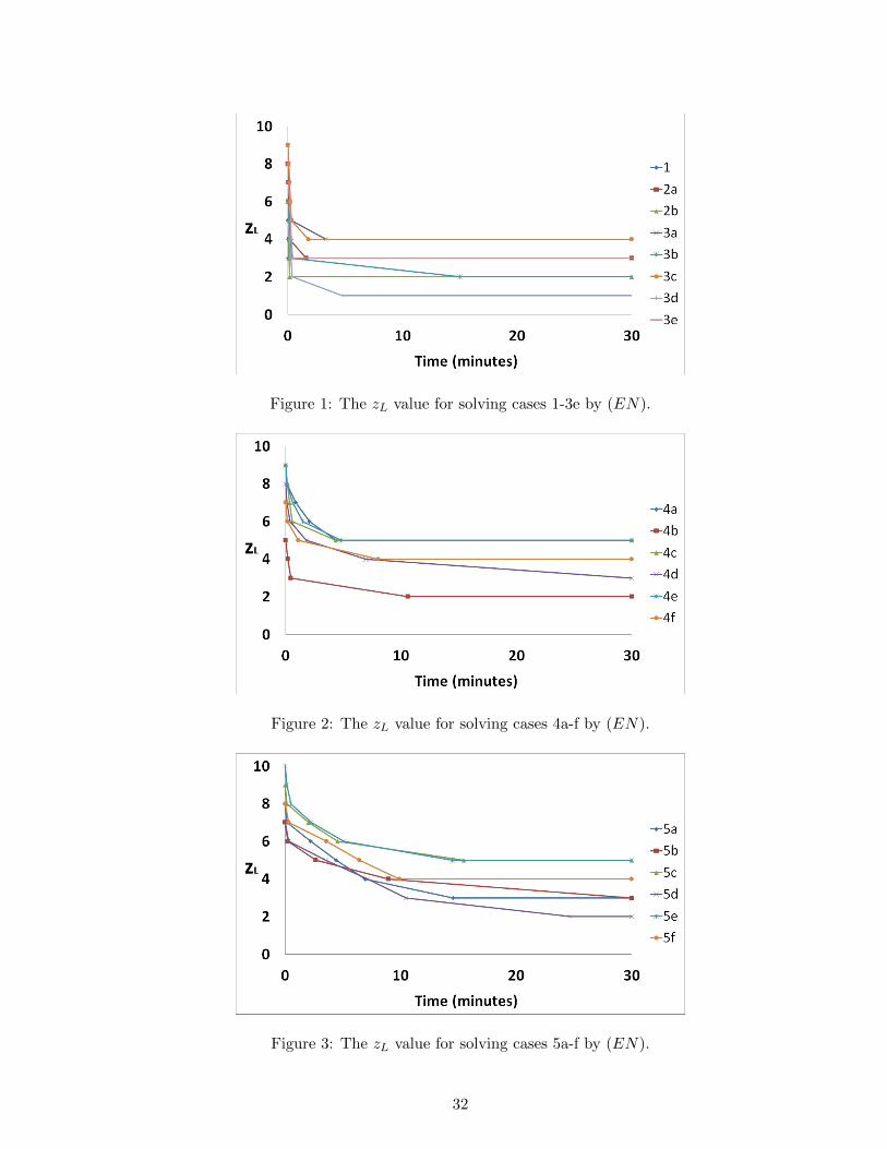
Figure 1: The zL value for solving cases 1-3e by (EN).

Figure 2: The zL value for solving cases 4a-f by (EN).

Figure 3: The zL value for solving cases 5a-f by (EN).

32

work shifts taking into account schedule fairness and staff preferences and the second phase is to

obtain a best-fit assignment of FSIs to tasks, in terms of skill-matches, at different locations and

create diversity of team formations. We also provide polyhedral results and devise valid inequal-

ities for the two formulations. After that, two exact algorithms to solve the two-phase problem

are developed. For the first-phase problem, we propose a relaxation with some fairness criteria

excluded to reduce the problem size so as to save computational effort in solving the LP relaxation.

The solution for the relaxation can be transformed easily into a feasible solution to the original

problem. We also provide an upper bound for the objective value of the relaxation. Computational

results show that the solutions produced are of good quality. For the second-phase problem, we

develop a shift-by-shift assignment heuristic to obtain an upper bound for the optimal zL value

and propose a zL-enumeration algorithm, which solves the staff-allocation problem with decreasing

values of zL. We also derive an optimality condition for the algorithm. The approach is efficient

since it avoids unnecessary computational effort for proving integer infeasibility for impossible zL

values, as verified by the computational experiments.

Acknowledgments

The research of the first author is partially supported by a grant from Asian Institute of Sup-

ply Chains and Logistics (Project No.: 8116027) and a grant from PROCORE: France/Hong Kong

Joint Research Scheme of Research Grant Council Hong Kong and the Consulate General of France

in Hong Kong (Project No.: 2900239). The research of the second author is supported by Microsoft

Research Asia Collaborative Research Fund (Grant No.: FY15-RES-THEME-049) and Macao Sci-

ence and Technology Development Fund (Grant No.: 088/2013/A3). The authors are grateful to

the operations manager of the food safety centre for providing information on the basic background

of their daily operations and first-hand knowledge of the constraints associated with scheduling

staff members. We are also indebted to the editors and the anonymous referees for their valuable

comments and suggestions.

Appendix

Proposition 1. Let (x1, z1W , z1H , z

1t ) be an optimal solution for (M1), (y2(x1), z2(x1)) be an optimal

solution for (M2) by taking x1 as an input and (x∗, z∗W , z∗H , z

∗t , y∗, z∗) be an optimal solution for

33

(IM), where x1 and x∗ are the vectors of the xis values, y2(x1) and y∗ are the vectors of the yisjl

values, and z2(x1) and z∗ are the vectors of the zi1i2sl and zL values. Then

wW z1W + wHz

1H +

∑t∈T

wtz1t +

∑i∈I,s∈S

wisx1is + wLz

2(x1)L +∑

i∈I,s∈S,j∈J,l∈Lwijy

2(x1)isjl

−

wW z∗W + wHz

∗H +

∑t∈T

wtz∗t +

∑i∈I,s∈S

wisx∗is + wLz

∗L +

∑i∈I,s∈S,j∈J,l∈L

wijy∗isjl

≤ wL|S|+ b

∑i∈I

maxj∈J

wij .

Proof Note that (x1, z1W , z1H , z

1t , 0, 0) is an optimal solution for the relaxation of (IM) which excludes

constraints (11) to (14). Thus

wW z1W + wHz

1H +

∑t∈T

wtz1t +

∑i∈I,s∈S

wisx1is

≤ wW z∗W + wHz

∗H +

∑t∈T

wtz∗t +

∑i∈I,s∈S

wisx∗is + wLz

∗L +

∑i∈I,s∈S,j∈J,l∈L

wijy∗isjl.

Moreover,

∑i∈I,s∈S,j∈J,l∈L

wijy2(x1)isjl ≤

∑i∈I,s∈S

maxj∈J

wij

∑j∈J,l∈L

y2(x1)isjl

=∑

i∈I,s∈Smaxj∈J

wijx1is

≤∑i∈I

maxj∈J

wijb.

Proof The second and final steps follow respectively from constraints (12) and (3). Finally, it is

trivial to see z2(x1)L ≤ |S|. �

Proposition 2. The constraint matrix formed by constraints (11) to (12) is TU.

Proof Note that a {0, 1} matrix A is TU if and only if for any subset R of the row indices, ∃

a partition (R1, R2) of R such that each column c satisfies |∑

r∈R1arc −

∑r∈R2

arc| ≤ 1, where

A = (arc). (Theorem 5.21 in Schrijver, 2003) By this fact, given a subset R, we construct a

partition (R1, R2) of R which satisfies this necessary and sufficient condition. We assign all row

indices of constraints (11) (if in R) to R1 and all row indices of constraints (12) (if in R) to R2.∑r∈R1

arc −∑

r∈R2arc ∈ {−1, 0, 1} for each column c. �

34

Proposition 3. Suppose S1, S2, ..., Sm are sets of shifts with d(s) = d(s′) ∀s, s′ ∈ Sk ∀1 ≤ k ≤ m

and {t(s1), t(s2), ..., t(sm)} is a prohibited sequence of shift types of consecutive days ∀s1 ∈ S1, s2 ∈

S2, ..., sm ∈ Sm. Then the following is a valid inequality for (M1).

m∑k=1

∑s∈Sk

xis ≤ m− 1 ∀i ∈ I (25)

Proof We show the inequality is valid by induction on day of shift and Chvatal-Gomory rounding

(Gomory, 1958; Chvatal, 1973) . For a fixed i ∈ I, suppose for some 0 ≤ q ≤ m − 1, ∀sq+1 ∈

Sq+1, sq+2 ∈ Sq+2, ..., sm ∈ Sm, the following inequality is valid.

q∑k=1

∑s∈Sk

xis +

m∑k=q+1

xisk ≤ m− 1

We assume∑q

k=1

∑s∈Sk

xis = 0 when q = 0, and thus, by inequality (5), the above inequality

is valid for q = 0.

The above inequality can be written as follows.

q∑k=1

∑s∈Sk

xis + xisq+1 +m∑

k=q+2

xisk ≤ m− 1

By summing up the above inequalities for all sq+1 ∈ Sq+1, we have

|Sq+1|q∑

k=1

∑s∈Sk

xis +∑

s∈Sq+1

xis + |Sq+1|m∑

k=q+2

xisk ≤ (m− 1)|Sq+1|.

By inequality (2), we have∑

s∈Sq+1xis ≤ 1. Summing up (|Sq+1| − 1)× (

∑s∈Sq+1

xis ≤ 1) and the

above inequality, we have

|Sq+1|

q+1∑k=1

∑s∈Sk

xis +m∑

k=q+2

xisk

≤ m|Sq+1| − 1.

and thus,q+1∑k=1

∑s∈Sk

xis +

m∑k=q+2

xisk ≤ m−1

|Sq+1|.

35

As the left-hand side is an integer, we have

q+1∑k=1

∑s∈Sk

xis +m∑

k=q+2

xisk ≤ m− 1.

Thus,∑q

k=1

∑s∈Sk

xis +∑m

k=q+1 xisk ≤ m− 1 implies∑q+1

k=1

∑s∈Sk

xis +∑m

k=q+2 xisk ≤ m− 1. We

repeat the procedure until q = m− 1 and so inequality (17) is valid. �

Theorem 1. Consider a polyhedron Q = {(u, v) ∈ Bm × Bm(m−1)/2 : uk1 + uk2 − vk1k2 ≤ 1

∀1 ≤ k1 < k2 ≤ m}, where m ≥ 2. Let M = {1, 2, ...,m}. Then the following inequalities are valid

for Q. ∑k∈M ′

uk −∑

k1,k2∈M ′:k1<k2

vk1k2 ≤ 1 ∀M ′ ⊆M, |M ′| ≥ 2 (26)

Proof W.L.O.G. let M ′ = {1, 2, ..., |M ′|}. Suppose the following inequality is valid for some 2 ≤

q < |M ′|.q∑

k=1

uk −∑

1≤k1<k2≤qvk1k2 ≤ 1 (27)

Note that, by the definition of Q, inequality (27) is valid for q = 2. By the definition of Q again,

uk + uq+1 − vk(q+1) ≤ 1 ∀1 ≤ k ≤ q

and thus, by summing up the above inequalities ∀1 ≤ k ≤ q,

q∑k=1

uk + quq+1 −q∑

k=1

vk(q+1) ≤ q.

Summing up (q − 1)× inequality (27) and the above inequality, we have

q

q+1∑k=1

uk − (q − 1)∑

1≤k1<k2≤qvk1k2 −

q∑k=1

vk(q+1) ≤ 2q − 1.

Dividing both sides by q and rounding down the coefficients on the left-hand side and the

right-hand side, we haveq+1∑k=1

uk −∑

1≤k1<k2≤q+1

vk1k2 ≤ 1.

Repeat the same procedure until q = |M ′| − 1. We have the desired inequality. �

36

Theorem 2. Consider the polyhedron Q in Theorem 1. Inequalities (18) are facet-defining inequal-

ities for Q.

Proof W.L.O.G. let M ′ = {1, 2, ..., |M ′|}. We are going to construct m+m(m−1)/2 feasible points

for Q, which are affinely independent and can satisfy inequality (18) with M ′ at equality.

There are four types of feasible points:

(i). For 1 ≤ k ≤ |M ′|, take uk = 1, 0 for other variables.

(ii). For |M ′| < k ≤ |M |, take u1 = uk = v1k = 1, 0 for other variables.

(iii). For 1 ≤ k1 < k2 ≤ |M ′|, take uk1 = uk2 = vk1k2 = 1, 0 for other variables.

(iv). For 1 ≤ k1 < |M |,max{k1, |M ′|} < k2 ≤ |M |, take u1 = vk1k2 = 1, 0 for other variables.

It is obvious that there are m + m(m − 1)/2 feasible points satisfying inequality (18) with M ′

at equality. To show the points are affinely independent, let α1k, α

2k, α

3k1k2

, α4k1k2

be some scalar

coefficients multiplied to the four types of feasible points respectively. The points are affinely

independent if and only if the following system does not have a non-zero solution.

|M ′|∑k=1

α1k +

|M ′|∑k=|M ′|+1

α2k +

|M ′|∑k1=1

|M |∑k2=k1+1

α3k1k2 +

|M |−1∑k1=1

|M |∑k2=max{k1,|M ′|}+1

α4k1k2 = 0

(u1) : α11 +

|M |∑k=|M ′|+1

α2k +

|M |∑k=2

α31k +

|M |−1∑k1=1

|M |∑k2=max{k1,|M ′|}+1

α4k1k2 = 0

(uk) : ∀2 ≤ k ≤ |M ′| α1k +

k−1∑k1=1

α3k1k +

|M ′|∑k2=k+1

α3kk2 = 0

∀|M ′| < k ≤ |M | α2k = 0

(v1k) : ∀2 ≤ k ≤ |M ′| α31k = 0

∀|M ′| < k ≤ |M | α2k + α4

1k = 0

(vk1k2) : ∀2 ≤ k1 < k2 ≤ |M ′| α3k1k2 = 0

∀2 ≤ k1 < |M |,max{k1, |M ′|} < k2 ≤ |M | α4k1k2 = 0

It is easy to see that the only solution to the above system is α1k, α

2k, α

3k1k2

, α4k1k2

= 0 ∀k, k1, k2.

Therefore the points are affinely independent and hence inequalities (18) are facet-defining. �

Corollary 1. The following inequality is valid for (M2).

37

∑i∈I′

∑j∈J

yisjl −∑

i1,i2∈I′:i1<i2

zi1i2sl ≤ 1 ∀I ′ ⊆ I, |I ′| ≥ 2, s ∈ S, l ∈ L (28)

Proof It follows directly from Theorem 1 and by inequalities (13). �

Proposition 4. The following inequality is valid for (M2).

zL ≥ maxI′⊆I,|I′|≥3,S′⊆S

d2(∑

i∈I′,s∈S′ xis − |S′||L|)|I ′|(|I ′| − 1)

e (29)

Proof Given I ⊆ I, |I ′| ≥ 3, and S′ ⊆ S, sum up valid inequalities (19) ∀s ∈ S′, l ∈ L to obtain

∑i∈I′,s∈S′,l∈L,j∈J

yisjl −∑

i1,i2∈I′:i1<i2,s∈S′,l∈Lzi1i2sl ≤ |S′||L|

and sum up constraints (14) ∀i1, i2 ∈ I ′ to obtain

∑i1,i2∈I′:i1<i2,s∈S,l∈L

zi1i2sl −|I ′|(|I ′| − 1)

2zL ≤ 0.

By summing up the above two inequalities and by constraints (12), we have

∑i∈I′,s∈S′

xis +∑

i1,i2∈I′:i1<i2,s∈S\S′,l∈L

zi1i2sl −|I ′|(|I ′| − 1)

2zL ≤ |S′||L|,

which leads to

zL −2

|I ′|(|I ′| − 1)

∑i1,i2∈I′:i1<i2,s∈S\S′,l∈L

zi1i2sl ≥2(∑

i∈I′,s∈S′ xis − |S′||L|)|I ′|(|I ′| − 1)

.

Rounding up the coefficients of the left-hand side and the right-hand side, and taking the maximum

among all I ′ ⊆ I and S′ ⊆ S, we obtain the required inequality. �

Proposition 5. Let (xR, zR) be an optimal solution for the relaxation (M1R). The objective value

contributed by the solution (xR, z(xR)) is bounded by twice the optimal objective value of (M1),

where z(xR) is defined as the maximum deviations among all the FSIs with respect to the solution

xR.

38

Proof Note that ∣∣∣∣∣∑s∈S

xRis −∑s∈S

xRi∗s

∣∣∣∣∣− zRW ≤ 0 ∀i ∈ I\{i∗}∣∣∣∣∣∣∑h∈H

∑s∈S:d(s)=h

xRis −∑h∈H

∑s∈S:d(s)=h

xRi∗s

∣∣∣∣∣∣− zRH ≤ 0 ∀i ∈ I\{i∗}

∣∣∣∣∣∣∑

s∈S:t(s)=t

xRis −∑

s∈S:t(s)=t

xRi∗s

∣∣∣∣∣∣− zRt ≤ 0 ∀t ∈ T, i ∈ I\{i∗}.

For i1, i2 ∈ I\{i∗},∣∣∣∣∣∑s∈S

xRi1s −∑s∈S

xRi2s

∣∣∣∣∣ =

∣∣∣∣∣∑s∈S

xRi1s −∑s∈S

xRi∗s +∑s∈S

xRi∗s −∑s∈S

xRi2s

∣∣∣∣∣≤

∣∣∣∣∣∑s∈S

xRi1s −∑s∈S

xRi∗s

∣∣∣∣∣+

∣∣∣∣∣∑s∈S

xRi∗s −∑s∈S

xRi2s

∣∣∣∣∣ ≤ 2zRW .

Similarly, we have

∣∣∣∣∣∣∑h∈H

∑s∈S:d(s)=h

xRi1s −∑h∈H

∑s∈S:d(s)=h

xRi2s

∣∣∣∣∣∣ ≤ 2zRH∣∣∣∣∣∣∑

s∈S:t(s)=t

xRi1s −∑

s∈S:t(s)=t

xRi2s

∣∣∣∣∣∣ ≤ 2zRt ∀t ∈ T.

Let (xO, zO) be an optimal solution for (M1).

wW z(xR)W + wHz(x

R)H +∑t∈T

wtz(xR)t +

∑i∈I,s∈S

wisxRis

= wW maxi1,i2∈I

∣∣∣∣∣∑s∈S

xRi1s −∑s∈S

xRi2s

∣∣∣∣∣+ wH maxi1,i2∈I

∣∣∣∣∣∣∑h∈H

∑s∈S:d(s)=h

xRi1s −∑h∈H

∑s∈S:d(s)=h

xRi2s

∣∣∣∣∣∣+∑t∈T

wt maxi1,i2∈I

∣∣∣∣∣∣∑

s∈S:t(s)=t

xRi1s −∑

s∈S:t(s)=t

xRi2s

∣∣∣∣∣∣+∑

i∈I,s∈Swisx

Ris

≤ 2(wW zRW + wHz

RH +

∑t∈T

wtzRt +

∑i∈I,s∈S

wisxRis)

≤ 2(wW zOW + wHz

OH +

∑t∈T

wtzOt +

∑i∈I,s∈S

wisxOis)

The last inequality follows from the fact that (xR, zR) is an optimal solution for a relaxation, and

39

therefore it gives a lower or equal objective value. �

Proposition 6. If wW , wH and wt >∑

i∈I,s∈S wis > 0 ∀t ∈ T , and ∃ an optimal solution (xO, 0)

for (M1), then an optimal solution (xR, zR) for (M1R) is an optimal solution for (M1).

Proof As (xR, zR) is an optimal solution for (M1R),

wW zRW + wHz

RH +

∑t∈T

wtzRt ≤ wW z

RW + wHz

RH +

∑t∈T

wtzRt +

∑i∈I,s∈S

wisxRis

≤ wW zOW + wHz

OH +

∑t∈T

wtzOt +

∑i∈I,s∈S

wisxOis

=∑

i∈I,s∈Swisx

Ois ≤

∑i∈I,s∈S

wis.

It is easy to see that zRW = zRH = 0 and zRt = 0 ∀t ∈ T . Otherwise, it contradicts the assumption

that 0 <∑

i∈I,s∈S wis < wW , wH and wt ∀t ∈ T . Note that (xR, 0) is also a feasible solution for

(M1) and thus ∑i∈I,s∈S

wisxOis ≤

∑i∈I,s∈S

wisxRis ≤

∑i∈I,s∈S

wisxOis.

Therefore, they have the same objective value. �

Proposition 7. If |I(s, S′)| > |L|, then zLs = 1.

Proof Summing up inequalities (24) ∀l ∈ L, we have

∑i∈I(s,S′),j∈J,l∈L

yijsl − |L|(|I(s, S′)| − 1)zLs ≤ |L|

|I(s, S′)| − |L| ≤ |L|(|I(s, S′)| − 1)zLs

|I(s, S′)| − |L||L|(|I(s, S′)| − 1)

≤ zLs.

As |I(s, S′)| > |L|, |I(s, S′)| − |L| ≤ |L|(|I(s, S′)| − 1) and zLs is integral, we have zLs = 1. �

Proposition 8. z∗L ≤ zL

Proof Note the optimal solution produced by the shift-by-shift assignment heuristic achieves the

lowest value of∑

i∈I,j∈J,s,∈S,l∈Lwijyijsl for the relaxation of (M2) which excludes constraints (13)

and (14) given the condition that 0 < |S|ε < mini∈I,j∈J wij . If zL < z∗L, then there exists a feasible

solution for (M2) with an objective lower than the optimal objective value, which leads to a con-

tradiction. �

40

Supplemental Material

The computational instances can be obtained from https://sites.google.com/site/yonghongkuo/research

or by emailing the authors.

References

[1] Aickelin, U., and Dowsland, K. A. (2004). An indirect genetic algorithm for a nurse-schedulingproblem. Computers and Operations Research, 31(5), 761–778.

[2] Alsheddy, A., and Tsang, E. P. (2011). Empowerment scheduling for a field workforce. Journalof Scheduling, 14(6), 639–654

[3] Al-Yakoob, S. M., and Sherali, H. D. (2007). Mixed-integer programming models for an employeescheduling problem with multiple shifts and work locations. Annals of Operations Research,155(1), 119–142.

[4] Asgeirsson, E. I. (2012). Bridging the gap between self schedules and feasible schedules in staffscheduling. Annals of Operations Research, 218(1),1–19.

[5] Awad, R. M., and Chinneck, J. W. (1998). Proctor Assignment at Carleton University. Inter-faces, 28(2), 58–71.

[6] Azaiez, M. N., and Al Sharif, S. S. (2005). A 0-1 goal programming model for nurse scheduling.Computers and Operations Research, 32(3), 491–507.

[7] Azmat, C. S., Hurlimann, T., and Widmer, M. (2004). Mixed integer programming to schedulea single-shift workforce under annualized hours. Annals of Operations Research, 128(1–4), 199–215.

[8] Bard, J. F. (2004). Staff scheduling in high volume service facilities with downgrading. IIETransactions, 36(10), 985–997.

[9] Bard, J. F., and Purnomo, H. W. (2005). Preference scheduling for nurses using column gener-ation. European Journal of Operational Research, 164(2), 510–534.

[10] Berrada, I., Ferland, J. A., and Michelon, P. (1996). A multi-objective approach to nursescheduling with both hard and soft constraints. Socio-Economic Planning Sciences, 30(3), 183–193.

[11] Billionnet, A. (1999). Integer programming to schedule a hierarchical workforce with variabledemands. European Journal of Operational Research, 114(1), 105–114.

[12] Burke, E. K., De Causmaecker, P., Berghe, G. V., and Van Landeghem, H. (2004). The stateof the art of nurse rostering. Journal of Scheduling, 7(6), 441–499.

[13] Cai, X., and Li, K. N. (2000). A genetic algorithm for scheduling staff of mixed skills undermulti-criteria. European Journal of Operational Research, 125(2), 359–369.

[14] Campbell, G. M. (1999). Cross-utilization of workers whose capabilities differ. ManagementScience, 45(5), 722–732.

41

[15] Campbell, G. M., and Diaby, M. (2002). Development and evaluation of an assignment heuristicfor allocating cross-trained workers. European Journal of Operational Research, 138(1), 9–20.

[16] Carrasco, R. C. (2010). Long-term staff scheduling with regular temporal distribution. Com-puter Methods and Programs in Biomedicine, 100(2), 191–199.

[17] Chvatal, V. (1973) Edmonds polytopes and a hierarchy of combinatorial problems. DiscreteMathematics, 4(4), 305–337.

[18] Cheang, B., Li, H., Lim, A., and Rodrigues, B. (2003). Nurse rostering problems – a biblio-graphic survey. European Journal of Operational Research, 151(3), 447–460.

[19] De Grano, M. L., Medeiros, D. J., and Eitel, D. (2009). Accommodating individual preferencesin nurse scheduling via auctions and optimization. Health Care Management Science, 12(3), 228–242.

[20] Eiselt, H. A., and Marianov, V. (2008). Employee positioning and workload allocation. Com-puters and Operations Research, 35(2), 513–524.

[21] Eitzen, G., Panton, D., and Mills, G. (2004). Multi-skilled workforce optimisation. Annals ofOperations Research, 127(1–4), 359–372.

[22] Ernst, A. T., Jiang, H., Krishnamoorthy, M., Owens, B., and Sier, D. (2004). An annotatedbibliography of personnel scheduling and rostering. Annals of Operations Research, 127(1–4),21–144.

[23] Ernst, A. T., Jiang, H., Krishnamoorthy, M., and Sier, D. (2004). Staff scheduling and roster-ing: A review of applications, methods and models. European Journal of Operational Research,153(1), 3–27.

[24] Fowler, J. W., Wirojanagud, P., and Gel, E. S. (2008). Heuristics for workforce planning withworker differences. European Journal of Operational Research, 190(3), 724–740.

[25] Gomory, R.E. (1958) Outline of an algorithm for integer solutions to linear programs. Bulletinof the American Mathematical Society, 64(5), 275–278.

[26] Kuo, Y. H., Leung, J. M.Y., and Yano, C. A. (2014). Scheduling of multi-skilled staff acrossmultiple locations. Production and Operations Management, 23(4), 626–644.

[27] Ladier, A. L., Alpan, G., and Penz, B. (2014). Joint employee weekly timetabling and dailyrostering: A decision-support tool for a logistics platform. European Journal of OperationalResearch, 234(1), 278–291.

[28] Maenhout, B., and Vanhoucke, M. (2010). A hybrid scatter search heuristic for personalizedcrew rostering in the airline industry. European Journal of Operational Research, 206(1), 155–167.

[29] Maenhout, B., and Vanhoucke, M. (2011). An evolutionary approach for the nurse rerosteringproblem. Computers and Operations Research, 38(10), 1400–1411.

[30] Mohan, S. (2008). Scheduling part-time personnel with availability restrictions and preferencesto maximize employee satisfaction. Mathematical and Computer Modelling, 48(11), 1806–1813.

[31] Parr, D., and Thompson, J. M. (2007). Solving the multi-objective nurse scheduling problemwith a weighted cost function. Annals of Operations Research, 155(1), 279–288.

42

[32] Rocha, M., Oliveira, J. F., and Carravilla, M. A. (2013). Cyclic staff scheduling: optimizationmodels for some real-life problems. Journal of Scheduling, 16(2), 231–242.

[33] Sabar, M., Montreuil, B., and Frayret, J. M. (2009). A multi-agent-based approach for per-sonnel scheduling in assembly centers. Engineering Applications of Artificial Intelligence, 22(7),1080–1088.

[34] Schrijver, A. (2003) Combinatorial optimization: polyhedra and efficiency. Vol. 24. Springer.

[35] Topaloglu, S. (2009). A shift scheduling model for employees with different seniority levels andan application in healthcare. European Journal of Operational Research, 198(3), 943–957.

[36] Van den Bergh, J., Belien, J., De Bruecker, P., Demeulemeester, E., and De Boeck, L. (2013).Personnel scheduling: A literature review. European Journal of Operational Research, 226(3),367–385.

[37] Warner, D. M. (1976). Scheduling nursing personnel according to nursing preference: A math-ematical programming approach. Operations Research, 24(5), 842–856.

[38] Wirojanagud, P., Gel, E. S., Fowler, J. W., and Cardy, R. (2007). Modelling inherent workerdifferences for workforce planning. International Journal of Production Research, 45(3), 525–553.

Biographies

Professor Chun-Hung CHENG obtained his PhD from the University of Iowa. While he was

a graduate student, he worked at the University of Iowa Hospital & Clinics as a programming

analyst. He started his teaching career at Kentucky State University. Later, he returned to Hong

Kong.

Professor Cheng’s research reflects his interest in Information Systems and Operations Man-

agement. His work has been published in internationally reputed journals, including the ACM

Transactions on Information Systems, Annals of Operations Research, Computers & Operations

Research, European Journal of Operational Research, Expert Systems, IEEE Transactions on En-

gineering Management, IEEE Transactions on Systems, Man, and Cybernetics, IIE Transactions,

Information and Management, Journal of Information Technology, Journal of Supply Chain Man-

agement, Omega, Operations Research, etc.

His earlier work (together with Professor WJ Boe) in a factory layout was implemented by a

third-party developer for toys manufacturers in South Brazil. He has recently led a project team to

design and implement operational systems for an air-mail center and two museums in Hong Kong.

He has also provided consulting services to local industries.

43

Dr. Yong-Hong Kuo is Research Assistant Professor in Stanley Ho Big Data Decision Analytics

Research Centre at the Chinese University of Hong Kong. He earned his B.Sc. in Mathematics

with a minor in Risk Management Science, and M.Phil. and Ph.D. in Systems Engineering and

Engineering Management, all from the Chinese University of Hong Kong. During his studies,

he worked at University of California at Berkeley as Visiting Researcher and Oak Ridge National

Laboratory as Research Student. Prior to returning to the Chinese University of Hong Kong, he was

Assistant Professor at the School of Business at Macau University of Science and Technology. His

research interests include operations research, combinatorial optimization, logistics management,

system simulation and healthcare management. His publications have appeared in internationally

reputed journals including IIE Transactions and Production and Operations Management.

44