Hypoplastic models for fine-grained soils A dissertation submitted for the Degree of Doctor of Philosophy David Maˇ s´ ın September 2006 Charles University, Prague Institute of Hydrogeology, Engineering Geology and Applied Geophysics

Welcome message from author
This document is posted to help you gain knowledge. Please leave a comment to let me know what you think about it! Share it to your friends and learn new things together.
Transcript
Hypoplastic models for fine-grained soils
A dissertation submitted for the
Degree of Doctor of Philosophy
David Masın
September 2006
Charles University, Prague
Institute of Hydrogeology, Engineering Geology and Applied Geophysics


Contents
1 Introduction 12
2 Hypoplastic model for clays 14
2.1 Introduction . . . . . . . . . . . . . . . . . . . . . . . . . . . . . . . . . . . . 14
2.2 Hypoplasticity . . . . . . . . . . . . . . . . . . . . . . . . . . . . . . . . . . 15
2.2.1 General aspects . . . . . . . . . . . . . . . . . . . . . . . . . . . . . . 15
2.2.2 Reference constitutive model . . . . . . . . . . . . . . . . . . . . . . 17
2.2.3 Intergranular strain concept . . . . . . . . . . . . . . . . . . . . . . . 17
2.3 Limitations . . . . . . . . . . . . . . . . . . . . . . . . . . . . . . . . . . . . 18
2.4 Proposed model . . . . . . . . . . . . . . . . . . . . . . . . . . . . . . . . . . 19
2.4.1 Tensor L . . . . . . . . . . . . . . . . . . . . . . . . . . . . . . . . . 19
2.4.2 Limit stress condition Y . . . . . . . . . . . . . . . . . . . . . . . . . 21
2.4.3 Hypoplastic flow rule (tensorial quantity m) . . . . . . . . . . . . . . 21
2.4.4 Barotropy factor fs . . . . . . . . . . . . . . . . . . . . . . . . . . . . 22
2.4.5 Pyknotropy factor fd . . . . . . . . . . . . . . . . . . . . . . . . . . . 23
2.4.6 Scalar factors c1 and c2 . . . . . . . . . . . . . . . . . . . . . . . . . 24
2.5 Inspection . . . . . . . . . . . . . . . . . . . . . . . . . . . . . . . . . . . . . 25
2.5.1 Shear moduli . . . . . . . . . . . . . . . . . . . . . . . . . . . . . . . 25
2.5.2 Stress–dilatancy behaviour . . . . . . . . . . . . . . . . . . . . . . . 29
2.5.3 Limitations of the proposed model . . . . . . . . . . . . . . . . . . . 30
2.6 Determination of parameters . . . . . . . . . . . . . . . . . . . . . . . . . . 30
2.6.1 Calibration of the HK model . . . . . . . . . . . . . . . . . . . . . . 32
2.7 Model predictions . . . . . . . . . . . . . . . . . . . . . . . . . . . . . . . . . 33
2.8 Conclusions . . . . . . . . . . . . . . . . . . . . . . . . . . . . . . . . . . . . 35
1

CONTENTS CONTENTS
3 State boundary surface 40
3.1 Introduction . . . . . . . . . . . . . . . . . . . . . . . . . . . . . . . . . . . . 40
3.2 Response envelopes and SOM states . . . . . . . . . . . . . . . . . . . . . . 41
3.3 Properties of the model . . . . . . . . . . . . . . . . . . . . . . . . . . . . . 43
3.4 Limit surface and Bounding surface . . . . . . . . . . . . . . . . . . . . . . . 44
3.5 Swept-out-memory surface . . . . . . . . . . . . . . . . . . . . . . . . . . . . 46
3.6 State boundary surface . . . . . . . . . . . . . . . . . . . . . . . . . . . . . . 49
3.7 Model performance . . . . . . . . . . . . . . . . . . . . . . . . . . . . . . . . 52
3.7.1 The influence of model parameters on the shape of the SOM surface 52
3.7.2 K0 normally compressed conditions . . . . . . . . . . . . . . . . . . 53
3.8 Concluding remarks . . . . . . . . . . . . . . . . . . . . . . . . . . . . . . . 54
4 Directional response 58
4.1 Introduction . . . . . . . . . . . . . . . . . . . . . . . . . . . . . . . . . . . . 58
4.2 Experimental data . . . . . . . . . . . . . . . . . . . . . . . . . . . . . . . . 60
4.3 Constitutive models considered . . . . . . . . . . . . . . . . . . . . . . . . . 62
4.3.1 The 3–SKH model . . . . . . . . . . . . . . . . . . . . . . . . . . . . 62
4.3.2 The CLoE hypoplastic model . . . . . . . . . . . . . . . . . . . . . . 62
4.3.3 The K-hypoplastic model for clays . . . . . . . . . . . . . . . . . . . 64
4.3.4 The K-hypoplastic model for clays with intergranular strain . . . . . 64
4.4 Model calibration . . . . . . . . . . . . . . . . . . . . . . . . . . . . . . . . . 65
4.4.1 Modified Cam-Clay model . . . . . . . . . . . . . . . . . . . . . . . . 66
4.4.2 3–SKH model . . . . . . . . . . . . . . . . . . . . . . . . . . . . . . . 68
4.4.3 CLoE hypoplastic model . . . . . . . . . . . . . . . . . . . . . . . . . 71
4.4.4 K-hypoplastic models for clays . . . . . . . . . . . . . . . . . . . . . 72
4.5 Comparison of predictions . . . . . . . . . . . . . . . . . . . . . . . . . . . . 75
4.5.1 Strain response envelopes . . . . . . . . . . . . . . . . . . . . . . . . 75
4.5.2 Normalized stress-paths . . . . . . . . . . . . . . . . . . . . . . . . . 76
4.5.3 Accuracy of directional predictions . . . . . . . . . . . . . . . . . . . 79
4.6 Concluding remarks . . . . . . . . . . . . . . . . . . . . . . . . . . . . . . . 83
5 The influence of OCR 93
5.1 Introduction . . . . . . . . . . . . . . . . . . . . . . . . . . . . . . . . . . . . 93
2

CONTENTS CONTENTS
5.2 Constitutive models . . . . . . . . . . . . . . . . . . . . . . . . . . . . . . . 94
5.3 Scalar error measure . . . . . . . . . . . . . . . . . . . . . . . . . . . . . . . 95
5.4 Calibration . . . . . . . . . . . . . . . . . . . . . . . . . . . . . . . . . . . . 97
5.4.1 The first group of parameters . . . . . . . . . . . . . . . . . . . . . . 97
5.4.2 The second group of parameters . . . . . . . . . . . . . . . . . . . . 98
5.5 Performance of the models . . . . . . . . . . . . . . . . . . . . . . . . . . . . 99
5.6 Concluding remarks . . . . . . . . . . . . . . . . . . . . . . . . . . . . . . . 102
6 Modelling meta-stable structure 104
6.1 Introduction . . . . . . . . . . . . . . . . . . . . . . . . . . . . . . . . . . . . 104
6.2 Reference model . . . . . . . . . . . . . . . . . . . . . . . . . . . . . . . . . 105
6.3 Conceptual approach . . . . . . . . . . . . . . . . . . . . . . . . . . . . . . . 106
6.4 Structure effects in hypoplasticity . . . . . . . . . . . . . . . . . . . . . . . . 107
6.5 Model performance and calibration . . . . . . . . . . . . . . . . . . . . . . . 111
6.6 Evaluation of model predictions . . . . . . . . . . . . . . . . . . . . . . . . . 113
6.7 Summary and conclusions . . . . . . . . . . . . . . . . . . . . . . . . . . . . 120
7 Comparison of hypoplasticity and elasto-plasticity 123
7.1 Introduction . . . . . . . . . . . . . . . . . . . . . . . . . . . . . . . . . . . . 123
7.2 Constitutive models . . . . . . . . . . . . . . . . . . . . . . . . . . . . . . . 124
7.2.1 Hypoplastic model for clays with meta-stable structure . . . . . . . 124
7.2.2 Structured modified Cam clay model . . . . . . . . . . . . . . . . . . 125
7.3 Evaluation . . . . . . . . . . . . . . . . . . . . . . . . . . . . . . . . . . . . . 125
7.4 Concluding remarks . . . . . . . . . . . . . . . . . . . . . . . . . . . . . . . 127
8 Summary and conclusions 130
9 Outlook 133
3
List of Tables
2.1 Summary of parameters of the basic version of the proposed model (left)and of the intergranular strain extension (right) for London clay. Standardvalues may be assumed for parameters in parenthesis . . . . . . . . . . . . . 31
2.2 Summary of parameters of the basic version of the HK model for London clay. 33
3.1 Parameters for London clay used in the simulations . . . . . . . . . . . . . . 53
4.1 Details of the experimental stress-probing program, after Costanzo et al. [31]. 61
4.2 Initial conditions assumed for the two sets of stress-probing tests . . . . . . 66
4.3 Parameters of the Modified Cam-Clay model. . . . . . . . . . . . . . . . . . 66
4.4 Parameters of the 3–SKH model. Quantities indicated with the symbol †have been assumed from data reported by Masın [86] for London Clay. . . . 69
4.5 Parameters of the CLoE model. Quantities indicated with the symbol † havebeen estimated according to Desrues [42]. . . . . . . . . . . . . . . . . . . . 72
4.6 Parameters of the K-hypoplastic models for clays. Quantities indicated withthe symbol † were assumed from data reported by Masın [86] for London Clay. 75
5.1 Material parameters . . . . . . . . . . . . . . . . . . . . . . . . . . . . . . . 99
6.1 Parameters of the proposed hypoplastic model for Pisa clay and Bothkennar
clay. . . . . . . . . . . . . . . . . . . . . . . . . . . . . . . . . . . . . . . . . 114
6.2 The initial values of the state variables for natural and reconstituted Pisa
clay and natural Bothkennar clay. . . . . . . . . . . . . . . . . . . . . . . . . 114
7.1 Parameters of the hypoplastic and SMCC models for Pisa and Bothkennarclays. . . . . . . . . . . . . . . . . . . . . . . . . . . . . . . . . . . . . . . . . 126
4

List of Figures
2.1 The influence of the stress factor 1/(T : T) (left) and the scalar quantity ξ(right) in the expression for L on the size and shape of response envelopes. 20
2.2 Definition of parameters N , λ∗ and κ∗ and quantities pcr and p∗e (from Sec.2.5). . . . . . . . . . . . . . . . . . . . . . . . . . . . . . . . . . . . . . . . . 25
2.3 Influence of the stress ratio η on the hypoelastic shear modulusG∗0 calculated
by the HK (left) and proposed (right) models with intergranular strains. . . 26
2.4 Erroneous increase of the shear stiffness calculated by the HK model en-hanced by the intergranular strain concept for the stress path passing isotropicstress state (left) and corresponding predictions by the proposed model withintergranular strains (right). . . . . . . . . . . . . . . . . . . . . . . . . . . . 26
2.5 Response envelopes of the proposed model (left) and HK model (right) withand without intergranular strains for isotropic stress states and for ϕmob =18◦ (with ϕc = 22.6◦) in triaxial compression and extension. . . . . . . . . . 28
2.6 Normalized stress paths of drained shear tests calculated by the HK (a) andproposed (b) models, with critical states indicated by points. Experimentalresults by Rampello and Callisto [114] on natural Pisa clay for qualitativecomparison (c). Simulations were performed with e = const., q = 0 kPa andvarying p. . . . . . . . . . . . . . . . . . . . . . . . . . . . . . . . . . . . . . 29
2.7 Calibration of parameters N , λ∗ and κ∗ on the basis of isotropic loadingand unloading test. Unlike the experiment, simulation started from normallycompressed state (left). Calibration of parameter r using a parametric study(right). . . . . . . . . . . . . . . . . . . . . . . . . . . . . . . . . . . . . . . 31
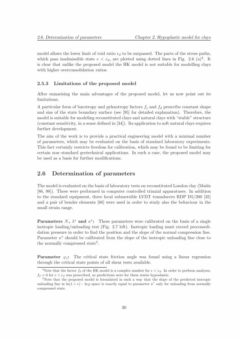
2.8 Calibration of parameter mR using linear regression on results from benderelement tests. . . . . . . . . . . . . . . . . . . . . . . . . . . . . . . . . . . 32
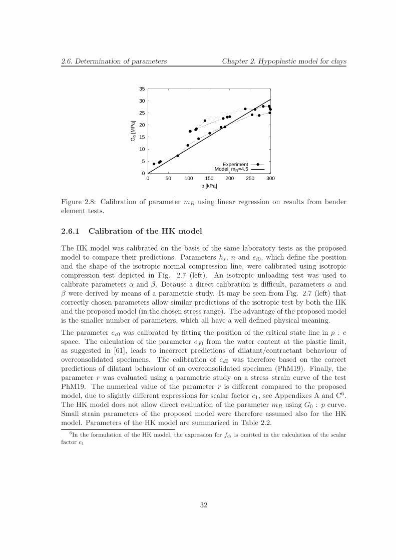
2.9 Stress–strain curves of three different compression tests. Experimental (left)and simulated (right). Simulation by the basic versions of the HK andproposed model. . . . . . . . . . . . . . . . . . . . . . . . . . . . . . . . . . 33
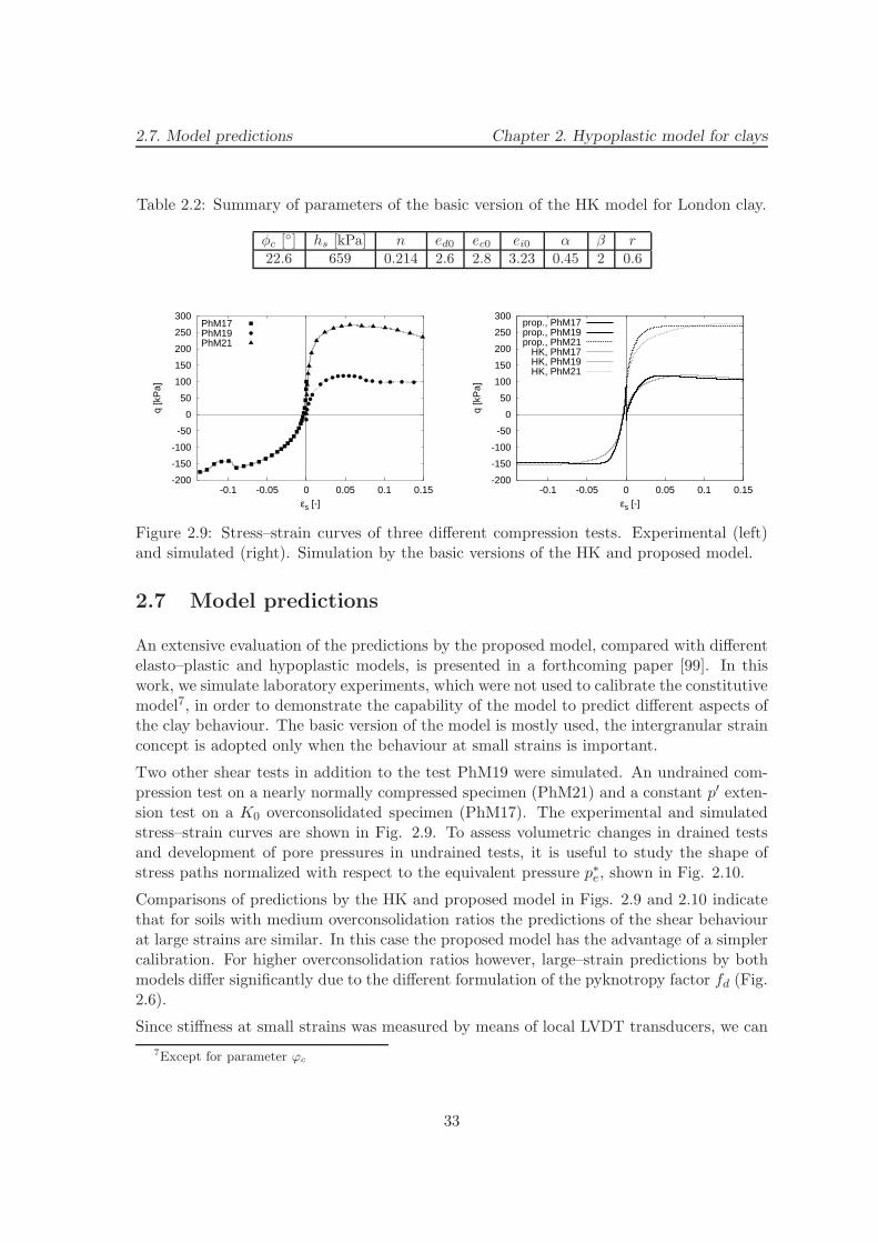
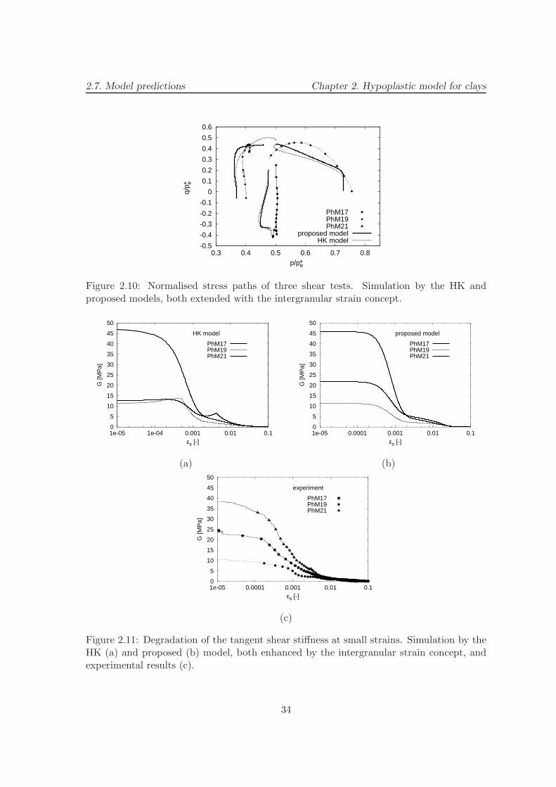
2.10 Normalised stress paths of three shear tests. Simulation by the HK andproposed models, both extended with the intergranular strain concept. . . 34
5

LIST OF FIGURES LIST OF FIGURES
2.11 Degradation of the tangent shear stiffness at small strains. Simulation bythe HK (a) and proposed (b) model, both enhanced by the intergranularstrain concept, and experimental results (c). . . . . . . . . . . . . . . . . . 34
2.12 Variation of bulk modulus in the isotropic unloading test with different de-grees of strain path rotation. Experiment and simulation by the proposedmodel with intergranular strains. . . . . . . . . . . . . . . . . . . . . . . . 35
3.1 On the definition of the incremental stress response envelope for the specialcase of axisymmetric conditions . . . . . . . . . . . . . . . . . . . . . . . . . 42
3.2 SOM-behaviour: proportional stress paths for proportional strain paths . . 42
3.3 Extended SOM-behaviour including void ratio . . . . . . . . . . . . . . . . . 43
3.4 Stress rate response envelopes for the initial stress located on the limit surface 46
3.5 On the definition of Hvorslev’s equivalent pressure p∗e. . . . . . . . . . . . . 47
3.6 Swept-out-memory surface in the normalised triaxial stress space for thehypoplastic model [87] using London clay parameters (Tab. 3.1) . . . . . . 49
3.7 NIREs for the initial K0NC conditions. (b) provides detail of (a). NIREs areplotted for R∆ǫ = 0.001, 0.0025, 0.005, 0.01, 0.02 (a) and R∆ǫ = 0.001 (b).Points at NIREs denote compression and extension for D00 = D11 = D22
and trD = 0) . . . . . . . . . . . . . . . . . . . . . . . . . . . . . . . . . . . 51
3.8 NIREs for the initial conditions with p/p∗e < 0.5, plotted for R∆ǫ = 0.001,0.005, 0.01, 0.02, 0.035. . . . . . . . . . . . . . . . . . . . . . . . . . . . . . 52
3.9 NIREs for the initial state outside the SOM surface. The initial state hasbeen imposed and does not follow from a model prediction. NIREs areplotted for R∆ǫ = 0.001, 0.0025, 0.005, 0.01, 0.02. . . . . . . . . . . . . . . . . 52
3.10 The influence of (a) the parameter ϕc and (b) of the ratio (λ∗−κ∗)/(λ∗+κ∗)on the shape of the SOM surface . . . . . . . . . . . . . . . . . . . . . . . . 54
3.11 K0NC conditions predicted by the considered model, compared to Jaky’s[66] formula and predictions by the Modified Cam clay model [117]. . . . . 55
4.1 Response envelope concept: a) input stress probes; b) output strain envelope. 61
4.2 Experimental stress-probes performed from state B . . . . . . . . . . . . . . 62
4.3 Sketch of the characteristic surfaces of the 3–SKH model . . . . . . . . . . . 63
4.4 Calibration of the Modified Cam-Clay model: a) determination of parame-ters N , λ and κ from isotropic compression and extension probes; b) deter-mination of critical state friction angle ϕc, from probes leading to failure; c)determination of elastic shear modulus, G, from the p = const. compressionprobe. . . . . . . . . . . . . . . . . . . . . . . . . . . . . . . . . . . . . . . . 67
6
LIST OF FIGURES LIST OF FIGURES
4.5 Calibration of the 3–SKH model: a) determination of parameter A fromdeviatoric probes; b) determination of parameter ψ from the p = const.compression probe. . . . . . . . . . . . . . . . . . . . . . . . . . . . . . . . . 69
4.6 Effect of initial position of kinematic hardening surfaces on the directionalresponse of 3–SKH model. a) Initial positions of kinematic surfaces assumedfor Cases (1) and (3); Strain response envelopes for axisymmetric probesfrom initial state A, and Rσ = 50 kPa. . . . . . . . . . . . . . . . . . . . . . 70
4.7 Initial configuration assumed for the kinematic surfaces of 3–SKH model: a)initial state A; b) initial state B. Stress probe directions are also shown inthe figures. . . . . . . . . . . . . . . . . . . . . . . . . . . . . . . . . . . . . 71
4.8 Calibration of the CLoE model: comparison of predicted and observed re-sponse for: a) conventional triaxial compression and extension tests, in theσa/σr:ǫa plane; b) conventional triaxial compression and extension tests, inthe ǫv:ǫa plane; c) isotropic compression and extension probes, in the ln(1+e):ln p plane; d) pseudo-isotropic compression test, in the ∆ǫa/∆ǫr : q/p plane. 73
4.9 Calibration of the K-hypoplastic model for clays: comparison of predictedand observed response for: a) isotropic compression and extension tests, inthe ln(1 + e):ln p plane; b) constant p triaxial compression, in the q:ǫs plane. 74
4.10 Experimental vs. simulated strain response envelopes for Rσ = 20, 30, 40and 50 kPa . . . . . . . . . . . . . . . . . . . . . . . . . . . . . . . . . . . . 77
4.11 Experimental vs. simulated strain response envelopes for Rσ = 50, and 90kPa . . . . . . . . . . . . . . . . . . . . . . . . . . . . . . . . . . . . . . . . 78
4.12 Experimental vs. simulated stress paths in the normalized plane q/p∗e:p/p∗e. 80
4.13 Scalar error measures with respect to the stress-path direction αpqσ in the p:qplane at state B, Rσ = 0 − 30 kPa . . . . . . . . . . . . . . . . . . . . . . . 82
4.14 Scalar error measures with respect to the stress-path direction αpqσ in the p:qplane at state B, Rσ = 0 − 90 kPa . . . . . . . . . . . . . . . . . . . . . . . 82
4.15 Experimental and predicted responses in the q:ǫs plane. . . . . . . . . . . . 87
4.16 Experimental and predicted responses in the p:ǫv plane. . . . . . . . . . . . 88
5.1 Characteristic surfaces of the 3-SKH model, from Masın et al., 2006. . . . . 94
5.2 Numerical values of err for experiments and simulations that differ only inincremental stiffnesses (left) and strain path directions (right). . . . . . . . 96
5.3 Approximation of experimental data for OCR = 10 by a polynomial function. 96
5.4 Calibration of parameters N , λ∗ and κ∗ of the CC model. . . . . . . . . . . 97
5.5 Calibration of ψ by means of minimalisation of err for experiment at OCR =10. . . . . . . . . . . . . . . . . . . . . . . . . . . . . . . . . . . . . . . . . . 98
7

LIST OF FIGURES LIST OF FIGURES
5.6 Predictions of the test OCR=10 by the 3SKH model with err-optimised(ψ = 2.53) and two different values of ψ. . . . . . . . . . . . . . . . . . . . . 99
5.7 err for parameters optimised for OCR = 1 (top) and OCR = 10 (bottom). 100
5.8 Peak friction angles ϕp predicted by the models with parameters optimisedfor OCR = 10. . . . . . . . . . . . . . . . . . . . . . . . . . . . . . . . . . . 101
5.9 Stress paths normalised by p∗e (a) and q vs. ǫs graphs (b) for OCR = 10optimised parameters. . . . . . . . . . . . . . . . . . . . . . . . . . . . . . . 102
5.10 ǫv vs. ǫs graphs for OCR = 10 optimised parameters. . . . . . . . . . . . . 103
6.1 Framework for structured fine-grained materials (Cotecchia and Chandler2000) . . . . . . . . . . . . . . . . . . . . . . . . . . . . . . . . . . . . . . . . 106
6.2 On definitions of the sensitivity s, Hvorslev equivalent pressure p∗e and ma-terial parameters N , λ∗ and κ∗. . . . . . . . . . . . . . . . . . . . . . . . . . 108
6.3 SOM surface of the hypoplastic model for clays for five different sets ofmaterial parameters (London clay – Masın 2005; Beaucaire marl – Masın etal. 2006; Kaolin – Hajek and Masın 2006; Bothkennar and Pisa clay – thisstudy.). . . . . . . . . . . . . . . . . . . . . . . . . . . . . . . . . . . . . . . 109
6.4 Response envelopes of the model with constant sensitivity (Si = 1), modelmodified only by multiplication of the factor fs by Si (case A) and modelwhere the physical meaning of parameters r and κ∗ is retained (case B). . . 110
6.5 Demonstration of the normalised incremental stress response envelopes foraxisymmetric conditions. . . . . . . . . . . . . . . . . . . . . . . . . . . . . . 111
6.6 Normalised incremental stress response envelopes of the proposed hypoplas-tic model plotted for medium (a) and large (b) strain range (R∆ǫ is in-dicated). The envelopes for the reconstituted material obtained with thereference hypoplastic model (Masın 2005) are also included. . . . . . . . . . 112
6.7 The influence of the parameter k (a) and A (b). . . . . . . . . . . . . . . . . 112
6.8 Calibration of the parameters N , λ∗ and κ∗ on the basis of an isotropiccompression test on reconstituted Pisa clay (a), parametric study for thecalibration of the parameter r (b). . . . . . . . . . . . . . . . . . . . . . . . 113
6.9 Calibration of parameters k (a) and A (b) using the structure degradationlaw of the hypoplastic model. . . . . . . . . . . . . . . . . . . . . . . . . . 115
6.10 Normalised stress paths of the natural and reconstituted Pisa clay (a) andpredictions by the hypoplastic model (b). . . . . . . . . . . . . . . . . . . . 116
6.11 Experiments on natural Pisa clay plotted in the ln(p/pr) vs. ln(1 + e) space(a) and predictions by the proposed hypoplastic model (b). . . . . . . . . . 116
6.12 ǫs vs. q diagrams of experiments on natural Pisa clay (a) and predictionsby the proposed hypoplastic model (b). . . . . . . . . . . . . . . . . . . . . 117
8

LIST OF FIGURES LIST OF FIGURES
6.13 Incremental strain response envelopes for R∆σ = ‖∆σ‖=10, 20, 30 (brokenline), 50 and 100 kPa, plotted together with strain paths in the
√2ǫr vs. ǫa
space. Experimental data on natural Pisa clay (a) and predictions by thehypoplastic model (b). . . . . . . . . . . . . . . . . . . . . . . . . . . . . . . 117
6.14 Normalised stress paths (a) and ǫs vs. q diagrams (b) of undrained com-pression (AUC) and extension (AUE) experiments on Pisa clay. . . . . . . . 118
6.15 Normalised stress paths of the natural and reconstituted Bothkennar clay(a) and predictions by the proposed hypoplastic model (b). . . . . . . . . . 119
6.16 Experiments on natural Bothkennar clay plotted in the ln(p/pr) vs. ln(1+e)space (a) and predictions by the proposed hypoplastic model (b). . . . . . . 119
6.17 ǫs vs. q diagrams of experiments on natural Bothkennar clay (a) and pre-dictions by the proposed hypoplastic model (b). . . . . . . . . . . . . . . . . 120
6.18 K0 tests on natural Bothkennar clay simulated with the hypoplastic modelusing two sets of material parameters. ”initial param.”: parameters opti-mized for predictions of LCD tests, ”adjust. param.”: modified value of theparameter k (k = 0.6) and lower initial sensitivity (s0 = 4). . . . . . . . . . 120
7.1 (a) Definitions of sensitivities sep and sh, quantities p∗c and p∗e and materialparameters N , λ∗ and κ∗. (b) Demonstration of similarity of the two struc-ture degradation laws on the basis of an isotropic compression test. pr is areference stress 1 kPa. . . . . . . . . . . . . . . . . . . . . . . . . . . . . . . 124
7.2 (a) Calibration of the parameters N , λ∗ and κ∗ of hypoplastic and SMCCmodels (isotropic compression test on reconstituted Pisa clay from Callisto1996); (b) Calibration of the parameter r of the hypoplastic model and Gof the SMCC model (data from Callisto and Calabresi 1998). . . . . . . . . 126
7.3 (a) normalised stress paths of the natural and reconstituted Pisa clay and(b) experiments on natural Pisa clay plotted in the ln(p/pr) vs. ln(1 + e)space. Experimental data and predictions by the hypoplastic and SMCCmodels. . . . . . . . . . . . . . . . . . . . . . . . . . . . . . . . . . . . . . . 127
7.4 (a) normalised stress paths and (b) ǫs vs. q curves from experiments on nat-ural Bothkennar clay. Experimental data and predictions by the hypoplasticand SMCC models. . . . . . . . . . . . . . . . . . . . . . . . . . . . . . . . . 128
9

Acknowledgements
The thesis would not have been written in this form without Prof. Ivo Herle and Dr.Jan Bohac. Ivo introduced me into numerical modelling in geomechanics and throughour numerous discussions guided my research activities, Jan originated my interest in soilmechanics and, particularly, managed to create perfect conditions for research at CharlesUniversity.
Although the research presented in the thesis was basically done in the period 2003 – 2006,it was initiated during my stay at City University. I would like to express my gratitude tothe staff of the Geotechnical engineering research centre, especially to Dr. S. E. Stallebrassand Prof. J. H. Atkinson.
I was lucky to work with many wise people who all left their traces in my research presentedin the thesis. Particularly I would like to thank to Prof. D. Kolymbas from the Universityof Innsbruck, Prof. C. Viggiani, Prof. C. Tamagnini, Prof. J. Desrues and Prof. R.Chambon, whom I met during my stay in Grenoble and Prof. G. Gudehus from theUniversity of Karlsruhe.
I thank to Dr. Luigi Callisto who provided data on Pisa clay, and to Prof. Mahdia Hattabfor making available the experimental results on Kaolin clay.
Finally, many thanks are due to all my other colleagues who contributed to my work, andto all my friends.
10
Abstract
Hypoplasticity has been shown to be a promising approach to constitutive modelling ofgeomaterials. An extensive research at universities in Karlsruhe and Grenoble led to thedevelopment of comprehensive constitutive models for granular materials. Much less effort,however, was put into the research on hypoplastic models for fine-grained soils. A newhypoplastic model suitable for description of clay behaviour is proposed in this dissertation.
The primary task was to develop a model suitable for practical applications – it shouldrequire minimum number of parameters, which can be evaluated using standard laboratoryprocedures. The proposed model requires only five parameters, equivalent to the parame-ters of the well-established Modified Cam clay model. In principle, only two experimentsare required for their evaluation – an isotropic loading and unloading test and a triaxialshear test. Void ratio is considered as a state variable and therefore, at least theoretically,a single set of material parameters may be used to predict the behaviour of soils withdifferent degrees of overconsolidation.
Tensorial analysis of the proposed model reveals that it predicts the state boundary surface,which is a natural ingredient of elasto-plastic models, but only a consequence of the mathe-matical formulation of hypoplastic models. A possibility to derive an analytical expressionof the state boundary surface is important for further developments of the model.
The thesis further brings an extensive evaluation of the proposed model. Two main as-pects are studied – predictions of the response to experiments with stress paths pointingin different directions in the stress space and predictions of the behaviour of soils withdifferent degrees of overconsolidation. The proposed model was in both cases comparedwith different advanced constitutive models, both elasto-plastic and hypoplastic. Althoughquantitative comparison of the quality of different models is a relatively complex task, pre-dictions by the proposed model were always at least comparable to predictions by the otheradvanced models tested.
Finally, a possibility for further development of the model is demonstrated by means ofincorporating the effects of structure in natural clays. An additional state variable – sensi-tivity – is a measure of the ratio of sizes of the state boundary surfaces of the reconstitutedand natural soil. A suitable evolution equation of it allows us to predict progressive changesin structure caused by degradation of cementation bonds.
11

Chapter 1
Introduction
Theory of hypoplasticity is a relatively recent approach to constitutive modelling of geoma-terials, developed independently during the last two decades at universities in Karlsruhe(e.g., [77]) and Grenoble [26, 29]. Initially, the research of both the schools focused onthe development of constitutive models for granular materials, the progress of hypoplasticmodels suitable for description of fine-grained soils has been delayed until recent years.
The hypoplastic models for fine-grained soils available when the present research started[105, 106, 61, 54] suffered from several shortcomings outlined in Chapter 2. The first aim ofthe present work was to develop a hypoplastic constitutive model for fine-grained soils thatwould be applicable in geotechnical practice, i.e. it should predict the behaviour of fine-grained soils with reasonable accuracy while requiring only minimum number of materialparameters. A further task was a study of some mathematical properties of the proposedmodel and its thorough evaluation with respect to experimental data. Finally, a possibilityto extend the basic formulation to describe the behaviour of materials with more complexstructure was studied.
The thesis consists of six main chapters, which are formed by research articles that appearedin different international journals and in conference proceedings.
The development of the new constitutive model is described step-by-step in Chapter 2. Thereference constitutive model by Herle and Kolymbas [61] is modified taking into accountprinciples set by Niemunis [106]. An evaluation of the proposed constitutive model withrespect to experimental data on London clay [86, 98, 126] is also presented (more detailedevaluation is given in Chapters 4 and 5). Chapter 2 was published as a research article inthe International Journal for Numerical and Analytical Methods in Geomechanics [87].
Some consequences of the mathematical structure of the new model are studied in Chap-ter 3. Tensorial analysis reveals that the model predicts existence of the so-called stateboundary surface, defined as a boundary of all admissible states in the stress-void ratiospace. Conclusions from Chapter 3 are important not only from the theoretical point ofview, but also for further development of the model (as demonstrated, e.g., in Chapter 6).Chapter 3, written by D. Masın and I. Herle, was published in Computers and Geotechnics
12

Chapter 1. Introduction
[97], a similar topic (together with the analysis of the hypoplastic model by von Wolffers-dorff [141]) was discussed by the same authors in Reference [96].
Chapter 4 presents an evaluation of predictive capabilities of the proposed model in com-parison with different advanced constitutive models, both elasto-plastic and hypoplastic.D. Masın, C. Tamagnini, G. Viggiani and D. Costanzo studied directional response of themodels (response to probes in different directions in the stress space from a common initialstate) and compared them with experimental results by Costanzo et al. [31]. Chapter 4 waspublished in the International Journal for Numerical and Analytical Methods in Geome-chanics [99], some selected results, together with description of the experimental evidence,can be found in Reference [130].
Further evaluation of the proposed model and comparison of its predictions with differentmodels is presented in Chapter 5 (V. Hajek and D. Masın, proceedings of the 6th EuropeanConference on Numerical Methods in Geomechanics [56]). Laboratory experiments (Hattaband Hicher [58]) were in this case characterised by identical stress paths directions (p’ con-stant tests), but started at different overconsolidation ratios. A range of overconsolidationratios for which a single set of material parameters can be used was studied.
Chapter 6 presents further development of the proposed model. Conclusions from Chapter 3and an existing framework for the mechanical behaviour of structured clays [34] are usedto enhance the basic hypoplastic model by additional state variable, sensitivity. A suitableevolution equation for sensitivity then allows us to predict the behaviour of clays with meta-stable structure. Chapter 6 has been accepted for publication in Canadian GeotechnicalJournal [88].
Predictions by the enhanced hypoplastic model are compared with its elasto-plastic ’equiv-alent’ (from the point of view of required material parameters) in Chapter 7. Advantageof the non-linear hypoplastic formulation is revealed. Chapter 7 is about to be publishedin proceedings of the International Workshop on Constitutive Modelling - Development,Implementation, Evaluation, and Application [90].
The last two chapters present a summary of the research and an outlook, where the pos-sibilities for further developments within hypoplastic framework are discussed.
13

Chapter 2
A hypoplastic constitutive modelfor clays
2.1 Introduction
In the past years many constitutive models based on the theory of hypoplasticity [77] havebeen developed for granular materials. This research, traced in Sec. 2.2.1, has led toconstitutive equations that can take into account the nonlinearity of the soil behaviour,the influence of barotropy and pyknotropy and also the behaviour at small to very smallstrains with the influence of the recent history of deformation [108].
The research into hypoplasticity, based at the University of Karlsruhe, was mainly focusedon the development of constitutive models for granular materials, such as sands or gravels.An important example is the model by von Wolffersdorff [141] (referred to in the followingtext “VW model”), which can be considered as a synthesis of the research work carriedout in Karlsruhe1 on this subject. Only a few attempts however have been made to applyhypoplastic principles to fine grained soils. A notable example are the visco–hypoplasticmodels by Niemunis [105, 109, 106]. These models assume logarithmic compression law [18]and, in line with the critical state soil mechanics [122], the lower limit for the void ratio eis equal to 0. Their formulation however concentrates on prediction of viscous effects and,since they arise from the model by von Wolffersdorff [141], it is not possible to specify theshear stiffness independently of the bulk stiffness and, as discussed by Herle and Kolymbas[61], the shear stiffness is significantly underpredicted.
A modification of the VW model, which allows for an independent calibration of the shearand bulk stiffnesses, was proposed by Herle and Kolymbas [61] (referred to in the followingas the “HK model”). In the HK model, Herle and Kolymbas modified the hypoelastictensor L (Sec. 2.2.1), which was responsible for the too low shear stiffness predicted by theVW model for soils with low friction angles, and introduced an additional model parameter
1There is also the second school of thought in the research on incrementally nonlinear models, Grenoble(e.g., [29]). This article however focuses on the developments of the German school.
14

2.2. Hypoplasticity Chapter 2. Hypoplastic model for clays
r controlling the ratio of shear and bulk moduli. This model however assumes the influenceof the barotropy and pyknotropy identical to the VW model, which is not suitable for clays.Moreover, the modification of the tensor L must vanish as the stress approaches the limitstate, which leads to incorrect predictions of the shear stiffness for anisotropic stress states(for further discussion see Sec. 2.3). The lack of a suitable hypoplastic formulation for finegrained soils led to the development of the model proposed in this paper.
In the following, the usual sign convention of solid mechanics (compression negative) isadopted throughout, except Roscoe’s variables p, q, ǫv and ǫs (e.g. [104]), which aredefined positive in compression. In line with the Terzaghi principle of effective stress, allstresses are effective stresses. Second–order tensors are denoted with bold letters (e.g.,T, m) and fourth–order tensors with calligraphic bold letters (e.g., L). Different types oftensorial multiplication are used: T ⊗ D = TijDkl, T : D = TijDij , L : D = LijklDkl,T · D = TijDjk. The quantity ‖X‖ =
√X : X denotes the Euclidean norm of X, the
operator arrow is defined as ~X = X/‖X‖ and trace by trX = X : 1. 1 is a second–orderunity tensor and I is a fourth order unity tensor with components Iijkl = 1
2 (1ik1jl + 1il1jk).
2.2 Hypoplasticity
2.2.1 General aspects
The hypoplastic constitutive equations are usually described by a simple non–linear tenso-rial equation that relates the objective (Jaumann) stress rate T with the Euler’s stretchingtensor D.
The early hypoplastic models were developed by trial and error, by choosing suitablecandidate functions (Kolymbas [75]) from the most general form of isotropic tensor–valuedfunctions of two tensorial arguments (representation theorem due to Wang [142]). Thesuitable candidate functions were combined automatically using a computer program thattested the capability of the constitutive model to predict the most important aspects of thesoil behaviour [76]. The research led to a practically useful equation with four parametersproposed by Wu [149] and Wu and Bauer [151].
As proven in [80], the hypoplastic equation may be written in its general form as
T = L : D + N‖D‖, (2.1)
where L and N are fourth and second–order constitutive tensors respectively that arefunctions of the Cauchy stress T only in the case of early hypoplastic models.
An important step forward in developing the hypoplastic model was the implementationof the critical state concept. Gudehus [53] proposed a modification of Eq. (2.1) to includethe influence of the stress level (barotropy) and the influence of density (pyknotropy). Themodified equation reads
T = fsL : D + fsfdN‖D‖. (2.2)
15

2.2. Hypoplasticity Chapter 2. Hypoplastic model for clays
Here fs and fd are scalar factors expressing the influence of barotropy and pyknotropy.The model [53] was later refined by von Wolffersdorff [141] to incorporate Matsuoka–Nakaicritical state stress condition.
A successful modification of the VW model is not straightforward due to the fact that theconstitutive tensors L and N are interrelated – they act together as a hypoplastic flowrule and limit stress condition. To overcome this problem, it is convenient to introduce thetensorial function
B = L−1 : N, (2.3)
which has been already used in the development of both Karlsruhe hypoplastic models [76]and CLoE hypoplastic models [29]. The Eq. (2.2) may be re–written,
T = fsL : (D + fdB‖D‖) . (2.4)
The critical state condition can be found by substituting T = 0 and fd = 1 into (2.4). Itfollows that T = 0 is satisfied trivially by D = 0 and for D 6= 0 by
~D = −B. (2.5)
Eq. (2.5) imposes a condition on stress, which can be revealed by elimination of ~D from(2.5). Taking the norm of both sides of (2.5) we obtain for the critical state
f = ‖B‖ − 1 = 0. (2.6)
The stress function f may be seen as a counterpart of the critical state stress criterion inelasto–plasticity [75]. A hypoplastic flow rule is then given by Eq. (2.5).
Using these transformations, Niemunis [106] proposed a simple rearrangement of the basichypoplastic equation (2.2), which allows definition of the flow rule, critical state stress con-dition and tensor L independently. Such a rearrangement is useful for model developmentand will also be used in this work.
The second–order tensor N is now calculated by
N = L :
(
−Y m
‖m‖
)
. (2.7)
Here the scalar quantity Y = f + 1 (named the degree of nonlinearity [106]) stands for alimit stress condition, m is a second–order tensor denoted hypoplastic flow rule and L isa fourth–order hypoelastic tensor from Eq. (2.2).
Eqs. (2.2) and (2.7) can be combined to get
T = fsL :
(
D− fdYm
‖m‖‖D‖)
. (2.8)
Eqs. (2.2) and (2.7), or Eq. (2.8), define the general stress–strain relationship of the modelproposed. Following [106], this formulation is named “generalised hypoplasticity”.
16

2.2. Hypoplasticity Chapter 2. Hypoplastic model for clays
2.2.2 Reference constitutive model
The HK model, introduced in Sec. 2.1, is taken as a reference model for the present researchand its mathematical formulation is summarised in Appendix A. The tensor L of the VWmodel is modified by introducing two scalar factors c1 and c2,
L =1
T : T
(
c1F2I + c2a
2T ⊗ T)
, (2.9)
where quantities T, F and a are defined in Appendix A. The expression for the factor c1 isderived in order to ensure that the additional model parameter r specifies the ratio of thebulk and shear moduli at isotropic stress state (details are given in Sec. 2.4.6) and factorc2 follows from the requirement that the isotropic formulations of both the HK and VWmodels merge,
c1 =
(
1 + 13a
2 − 1√3a
1.5r
)ξ
, c2 = 1 + (1 − c1)3
a2. (2.10)
Because the HK model does not make use of the generalised hypoplasticity formulation (Sec.2.2.1), the influence of fators c1 and c2 must vanish as the stress approaches Matsuoka–Nakai critical state stress criterion. For this reason, a scalar factor ξ is introduced in theformulation of the factor c1 (Eq. (2.10)), which reads
ξ =
⟨
sinϕc − sinϕmobsinϕc
⟩
, where sinϕmob =T1 − T3
T1 + T3. (2.11)
T1 and T3 are the maximal and minimal principal stresses, ϕmob is a mobilized frictionangle and 〈〉 are Macauley brackets: 〈x〉 = (x+ |x|)/2.
2.2.3 Intergranular strain concept
The hypoplastic models discussed in previous sections are capable of predicting the soilbehavior upon monotonic loading at medium to large strain levels. In order to preventexcessive ratcheting upon cyclic loading and to improve model performance in the small–strain range, the mathematical formulation has been enhanced by the intergranular strainconcept [108].
The rate formulation of the enhanced model is given by
T = M : D, (2.12)
where M is the fourth–order tangent stiffness tensor of the material. The formulationintroduces the additional state variable δ, which is a symmetric second order tensor calledintergranular strain.
In the formulation described above, the total strain can be thought of as the sum of acomponent related to the deformation of interface layers at integranular contacts, quantified
17

2.3. Limitations Chapter 2. Hypoplastic model for clays
by δ, and a component related to the rearrangement of the soil skeleton. For reverseloading conditions (δ : D < 0, where δ is defined in Appendix B) and neutral loadingconditions (δ : D = 0), the observed overall strain is related only to the deformation of theintergranular interface layer and the soil behaviour is hypoelastic, whereas in continuousloading conditions (δ : D > 0) the observed overall response is also affected by particlerearrangement in the soil skeleton. From the mathematical standpoint, the response of themodel is determined by interpolating between the following three special cases:
T = mRfsL : D, for δ : D = −1 and δ = 0;
T = mT fsL : D, for δ : D = 0;
T = fsL : D + fsfdN‖D‖, for δ : D = 1.
(2.13)
Full details of the mathematical structure of the model are provided in Appendix B. Themodel, which incorporates the intergranular strain concept is in the paper denoted as“enhanced”, the model without this modification as “basic”.
2.3 Limitations of the reference model
As pointed out in the introduction, although the HK model improved predictions of the claybehaviour significantly, several shortcomings may still be identified. The most importantare:
• Measurements of the shear stiffness at very small strains (G0), by means of prop-agation of shear waves, allows investigation of the dependence of G0 on the stresslevel. For clays such studies were performed for example in [139, 69, 135, 22]. It wasshown that for stresses inside the limit state surface G0 depends on the mean stressp but the influence of the deviatoric stress q is not significant (both for triaxial com-pression and extension). The HK model with intergranular strains however predictssignificant decrease of the hypoelastic shear modulus G0 with the ratio η = q/p, asdiscussed in Sec. 2.5 (Figs. 2.3 and 2.4).
• The HK model assumes a non–zero, pressure–dependent lower limit of void ratio,ed. While this approach is suitable for granular materials, for clays it is reasonableto consider the lower limit of void ratio of e = 0, according to the critical statesoil mechanics [122], supported by experimental studies on the shape of the stateboundary surface of fine–grained soils (e.g., [32, 33, 34]). Taking the pyknotropyfactor fd a function of relative density re calculated by
re =e− edec − ed
, (2.14)
with ec being void ratio at the critical state line at current mean stress, leads toincorrect predictions of the stress–dilatancy behaviour by the HK model (for detailssee Sec. 2.5, Fig. 2.6), also for the case when lower limit of void ratio e = 0 isprescribed (ed0 = 0).
18

2.4. Proposed model Chapter 2. Hypoplastic model for clays
• The HK model adopts exponential expressions for the isotropic normal compressionand critical state lines [10]. Compared to the logarithmic expression, the exponentialexpression has the advantage of having limits for p → 0 and p → ∞. For clayshowever the logarithmic expression is more accurate in the stress range applicablein geotechnical engineering [18], with the further advantage of having one materialparameter less.
• Taking into account the desired simplicity of the calibration of the proposed model,the parameter defining the position of the critical state line in the e : p plane (ec0)may be regarded as superfluous. For clays the position of the critical state linecalculated using the state boundary surface of the Modified Cam clay model [117] issufficiently accurate, as shown recently for different clays in [32, 33, 34].
• The HK model does not allow specifying directly the swelling index, κ∗. The slope ofthe isotropic unloading line is governed by two parameters, α and β. Direct evaluationof these parameters from isotropic unloading test is complicated and the calibrationis usually performed by means of a parametric study.
The proposed hypoplastic model for clays aims at overcoming the outlined shortcomingsof the HK model and achieving maximal simplicity of the calibration of the new model,which is desired in practical applications.
2.4 Proposed constitutive model
2.4.1 Tensor L
The tensor L (Eq. (2.9)) determines, in the model enhanced by the intergranular strainconcept (Sec. 2.2.3), the initial hypoelastic stiffness and causes the HK model to predict adecrease of the initial shear modulus G0 with the stress ratio η, which is not in agreementwith experiment (see Sec. 2.3). The influence of η on G0 is caused by the factor 1/(T : T)(where T = T/trT), the decrease of the scalar quantity ξ as the stress approaches limitstate and the factor F , which increases the compressibility for Lode angles different thanπ/6.
The influence of the first two factors is studied using the concept of incremental responseenvelopes [134]. This concept follows directly from the concept of rate response envelope[50], with rates replaced by finite–size increments with constant direction of stretching ~D(for brevity, incremental response envelopes are referred to as response envelopes in thiswork). Response envelopes are plotted for ∆t‖D‖ = 0.0015, where t is pseudo–time usedfor time integration of the model response. The HK model enhanced by the intergranularstrain concept is used in the simulations, modified by either keeping 1/(T : T) = const. = 3or η = const. = 1 (Fig. 2.1). The initial value of the intergranular strain tensor δ is equalto 0.
19

2.4. Proposed model Chapter 2. Hypoplastic model for clays
0
50
100
150
200
250
300
350
400
0 50 100 150 200 250 300 350 400
-√2T
33 [k
Pa]
-T11 [kPa]
stress factor=3with stress factor
0
50
100
150
200
250
300
350
400
0 50 100 150 200 250 300 350 400
-√2T
33 [k
Pa]
-T11 [kPa]
ξ=1ξ dec. with ϕmob
Figure 2.1: The influence of the stress factor 1/(T : T) (left) and the scalar quantity ξ(right) in the expression for L on the size and shape of response envelopes.
It may be seen From Fig. 2.1 (left) that the influence of the stress quantity 1/(T : T) is notsignificant. In the VW model this quantity was introduced in order to emphasize that theoverall compressibility of sand is larger at higher stress ratios. For clays it is well knownthat the normal compression lines are approximately parallel for different radial stresspaths (as isotropic and K0 normal compression lines and critical state line). FollowingNiemunis [106], the factor 1/(T : T) may be disregarded and in the present model it isreplaced by its isotropic value equal to 3.
Fig. 2.1 (right) shows that the influence of the factor ξ, which in the HK model mustdecrease with ϕmob in order to ensure that the model predicts correctly the critical state(Sec. 2.2.2), is very significant. The response envelopes become narrower as the stressapproaches the critical state and the initial shear modulus G0 decreases significantly. Theproposed model therefore does not make use of the quantity ξ and so constant values ofscalar factors c1 and c2 (Sec. 2.2.2) are assumed. This modification is enabled by adoptingthe generalised hypoplastic formulation (Sec. 2.2.1).
In the VW model the factor F had to enter the expression for L to ensure that the functionB conforms with the Matsuoka–Nakai failure criterion. As quoted in Sec. 2.3, accordingto experiments on fine–grained soils, G0 is independent of η in both triaxial compressionand extension [139]. Therefore, the factor F should be in the expression for L omitted.
We assume the following formulation of the hypoelastic tensor L:
L = 3(
c1I + c2a2T ⊗ T
)
. (2.15)
The calculation of scalar factors c1 and c2, which follows [61], is described in Sec. 2.4.6.The scalar factor a is a function of material parameter ϕc and follows from VW model,
a =
√3 (3 − sinϕc)
2√
2 sinϕc. (2.16)
20

2.4. Proposed model Chapter 2. Hypoplastic model for clays
2.4.2 Limit stress condition Y
As shown, for example, in [73, 20, 114] the Drucker–Prager critical state stress criterion,which is assumed also by the Modified Cam clay model, is not suitable for clays. The actualcritical state stress criterion circumscribes the Mohr–Coulomb criterion with approximatelyequal friction angles in triaxial compression and extension.
Therefore, the Matsuoka–Nakai [85] criterion assumed by the VW hypoplastic model isapplicable also for clays. It is described by the equation
f = − I1I2I3
− 9 − sin2 ϕc
1 − sin2 ϕc≤ 0, (2.17)
with the stress invariants
I1 = trT, I2 =1
2
[
T : T − (I1)2]
, I3 = detT. (2.18)
As pointed out by Niemunis [106], the quantity Y should have a minimum value at theisotropic axis (maximum Y = 1 at the critical state stress criterion). Direct linear inter-polation between the isotropic value Y = Yi and limit state value Y = 1 is assumed in theproposed model, following [106].
Using the fact that I1I2/I3 = −9 at the hydrostatic stress state, the linear interpolationreads
Y = (1 − Yi)
− I1I2I3
− 9
9 − sin2 ϕc
1 − sin2 ϕc− 9
+ Yi, (2.19)
with Yi being equal to the isotropic value of the function ‖B‖ of the VW (HK) model,
Yi =
√3a
3 + a2. (2.20)
2.4.3 Hypoplastic flow rule (tensorial quantity m)
~m = m/‖m‖ is a tensorial function that should have purely volumetric direction atisotropic stress state and purely deviatoric direction (tr m = 0) at Matsuoka–Nakai states,
{
~m = −T∗/‖T∗‖, for Y = 1;
~m = − 1√31, for Y = Yi,
(2.21)
where the stress quantity T∗
is defined as T∗
= T − 1/3. A suitable candidate is thefunction −B of the VW hypoplastic model [141],
m = − a
F
[
T + T∗ − T
3
(
6 T : T − 1
(F/a)2 + T : T
)]
, (2.22)
21

2.4. Proposed model Chapter 2. Hypoplastic model for clays
with factor F defined by
F =
√
1
8tan2 ψ +
2 − tan2 ψ
2 +√
2 tanψ cos 3θ− 1
2√
2tanψ, (2.23)
where
tanψ =√
3‖T∗‖, cos 3θ = −√
6tr(
T∗ · T∗ · T∗)
[
T∗
: T∗]3/2
. (2.24)
Note that the adopted formulation of the function m implies radial strain increments inoctahedral plane at the critical state. For fine–grained soils this choice is supported by theexperimental evidence given by Kirkgard and Lade [73].
2.4.4 Barotropy factor fs
The aim of the barotropy factor fs is to incorporate the influence of the mean stressp = −trT/3. The calculation of the factor fs is based on the formulation of the pre–defined isotropic normal compression line.
The proposed model assumes isotropic normal compression line linear in the ln(1+e) : ln pspace, which is suitable for clays [18]. Its position is governed by the parameter N and itsslope by the parameter λ∗,
ln(1 + e) = N − λ∗ ln p. (2.25)
Time differentiation of (2.25) results in
e
1 + e= − λ∗
pp. (2.26)
The already defined quantities L, m and Y , together with the yet unknown values ofpyknotropy factor fd at the isotropic normally compressed state (fdi) and the factors c1and c2, may be used to derive the form of the Eq. (2.7) for isotropic stress state. With theuse of
p = − 1
3trT, D =
e
3 (1 + e)1, and ‖D‖ =
|e|3 (1 + e)
√3, (2.27)
we find
p = − fs3 (1 + e)
(
3c1 + a2c2)
[
e+ fdia√
3
3 + a2|e|]
. (2.28)
As discussed in Sec. 2.2.2, calculation of the scalar factor c2, introduced in [61], ensuresthat the modification of the tensor L does not influence the isotropic formulation of themodel. Therefore it follows from (2.28) that
3c1 + a2c2 = 3 + a2. (2.29)
22

2.4. Proposed model Chapter 2. Hypoplastic model for clays
Eq. (2.28) may be therefore simplified to
p = − 1
3 (1 + e)fs
[
(
3 + a2)
e+ fdia√
3|e|]
, (2.30)
and for isotropic compression with e < 0
p = −[
1
3 (1 + e)fs
(
3 + a2 − fdia√
3)
]
e. (2.31)
Comparing (2.26) with (2.31) we derive the expression for the barotropy factor fs,
fs = − trT
λ∗
(
3 + a2 − fdia√
3)−1
. (2.32)
2.4.5 Pyknotropy factor fd
The pyknotropy factor fd was introduced in [53] in order to incorporate the influence ofdensity (overconsolidation ratio) on the soil behaviour. If we assume, following discussionin Sec. 2.3, that the lower limit of void ratio is e = 0 for clays, the pyknotropy factor fdhas the following properties:
• fd = 0 for p = 0;
• fd = 1 at the critical state;
• fd = const. > 1 at isotropic normally compressed states.
Moreover, the pyknotropy factor fd should have constant value along any other normalcompression line (reasons for this choice are demonstrated in [95]). Taking into accountthe outlined properties of the factor fd, we propose a simple expression
fd =
(
p
pcr
)α
, (2.33)
where pcr is the mean stress at the critical state line at the current void ratio (Fig. 2.2).
As discussed in Section 2.3, the position of the critical state line in ln(1 + e) : ln p spacedoes not need to be controlled by an additional parameter, since for clays this positionis sufficiently accurately defined by the state boundary surface of the Modified Cam claymodel. The expression for the critical state line reads
ln(1 + e) = N − λ∗ ln 2pcrpr, (2.34)
where pr is the reference stress 1 kPa. Therefore,
fd =
[
− 2trT
3prexp
(
ln (1 + e) −N
λ∗
)]α
. (2.35)
23

2.4. Proposed model Chapter 2. Hypoplastic model for clays
The scalar quantity α is calculated to allow for a direct calibration of the swelling indexκ∗, defined as the slope of the isotropic unloading line in the ln(1 + e) : ln p space. Thisline has the expression
ln(1 + e) = const. − κ∗ ln p, (2.36)
which leads after time differentiation to
e
1 + e= − κ∗
pp. (2.37)
For isotropic unloading from the isotropic normally compressed state the proposed modelhas the form (from Eq. (2.30))
p = −[
1
3 (1 + e)fs
(
3 + a2 + fdia√
3)
]
e. (2.38)
Having defined the barotropy factor fs (2.32) and the pyknotropy factor for the isotropicnormally compressed state fdi (from Eqs. (2.35) and (2.25)),
fdi = 2α, (2.39)
we may rewrite Eq. (2.38) to get
p = −[
p
λ∗ (1 + e)
(
3 + a2 + 2αa√
3
3 + a2 − 2αa√
3
)]
e. (2.40)
Comparing (2.40) with (2.37) we derive the expression for the scalar quantity α,
α =1
ln 2ln
[
λ∗ − κ∗
λ∗ + κ∗
(
3 + a2
a√
3
)]
. (2.41)
The meaning of the model parameters N , λ∗ and κ∗ is demonstrated in Fig. 2.2.
2.4.6 Scalar factors c1 and c2
Calculation of the factor c2 is based on Eq. (2.29) and follows [61],
c2 = 1 + (1 − c1)3
a2. (2.42)
For the calculation of the factor c1, we define the constitutive parameter r as the ratio ofthe bulk modulus in isotropic compression (Ki) and the shear modulus in undrained shear(Gi) for tests starting from the isotropic normally compressed state. Manipulation withthe proposed model leads to expressions for Ki and Gi,
Ki =fs3
(
3 + a2 − 2αa√
3)
, (2.43)
Gi =3
2fsc1. (2.44)
24

2.5. Inspection Chapter 2. Hypoplastic model for clays
pe*crp
*λ
*κ
Critical state line
ln p
ln (1+e)
Isotr. normal compression line
N
current stateIsotr. unloading line
1
1
Figure 2.2: Definition of parameters N , λ∗ and κ∗ and quantities pcr and p∗e (from Sec.2.5).
Because r = Ki/Gi, we find
c1 =2(
3 + a2 − 2αa√
3)
9r. (2.45)
Having obtained factors c1 and c2, the mathematical formulation of the proposed model iscomplete. It is summarized in Appendix C. The model requires five constitutive parame-ters: ϕc, λ
∗, κ∗, N and r.
2.5 Inspection into properties of the model
2.5.1 Shear moduli
A significant shortcoming of the HK model is the underprediction of the initial shear stiff-ness G0 for tests starting from anisotropic stress states. This deficiency is very importantfor practical applications, since the stress state in the field is often anisotropic.
Using the intergranular strain concept (Sec. 2.2.3), the quasi–elastic behaviour is controlledby the equation
T = mRfsL : D. (2.46)
In the following, we restrict our attention only to axisymmetric conditions, as we want toexamine possibility of calibration of model parameters, not to provide a full analysis ofmodel performance. We may define the shear modulus G∗ using Roscoe’s variables p, q, ǫvand ǫs (e.g., [104]) as follows [47]:
[
pq
]
=
[
K∗ JJ 3G∗
] [
ǫvǫs
]
. (2.47)
25

2.5. Inspection Chapter 2. Hypoplastic model for clays
0
5
10
15
20
25
30
35
40
0 50 100 150 200 250 300 350 400
G* 0
[MP
a]
p [kPa]
η=0η=0.5
0
5
10
15
20
25
30
35
40
45
0 50 100 150 200 250 300 350 400
G* 0
[MP
a]
p [kPa]
η=0η=0.5
Figure 2.3: Influence of the stress ratio η on the hypoelastic shear modulus G∗0 calculated
by the HK (left) and proposed (right) models with intergranular strains.
0
5
10
15
20
1e-05 1e-04 0.001 0.01 0.1
G [M
Pa]
-εs [kPa]
0
5
10
15
20
1e-05 1e-04 0.001 0.01 0.1
G [M
Pa]
-εs [kPa]
-150-100-50
0 50
100 150
0 100 200 300
q [k
Pa]
p [kPa]
Figure 2.4: Erroneous increase of the shear stiffness calculated by the HK model enhancedby the intergranular strain concept for the stress path passing isotropic stress state (left)and corresponding predictions by the proposed model with intergranular strains (right).
26

2.5. Inspection Chapter 2. Hypoplastic model for clays
Because the hypoelastic stiffness tensor L is not isotropic, G∗ is equal to the equivalentshear modulus defined by G = q/(3ǫs) only for undrained conditions.
Combining (2.46) and (2.47) we find that
G∗0 =
mRfs3
[
L1111 − 2L2211 +1
2(L2222 + L2233)
]
. (2.48)
Substituting expressions for L (2.15) and fs (2.32) we get
G∗0 =
mRp
3λ∗(
3 + a2 − 2αa√
3)
[
27
2c1 +
c2a2
p2
(
T 211 − 2T22T11 +
1
2T 2
22 +1
2T22T33
)]
, (2.49)
and therefore
G∗0 =
mRp
3λ∗(
3 + a2 − 2αa√
3)
(
27
2c1 + c2a
2η2
)
. (2.50)
Eq. (2.50) shows that the modulus G∗0 predicted by the proposed model depends both on
the mean stress p and stress ratio η. The second term in parenthesis in (2.50) is howeversignificantly smaller, than the first term (for parameters derived in Sec. 2.6 and η = 0.5the first term is 13.2 times larger). Therefore, contrary to the HK model, the influence ofη on G∗
0 is not significant. This observation is shown in Fig. 2.3 (right), with predictionsby the HK model in Fig. 2.3 (left) for comparison. This drawback of the formulation ofHK model is also demonstrated in Fig. 2.4 (left). The initial stiffness for the stress path,which starts at anisotropic stress state and passes isotropic stress state, is underpredictedand the model predicts unrealistic increase of the tangent stiffness at isotropic conditions.The improved prediction by the proposed model is in Fig. 2.4 (right).
As follows from Fig. 2.3 (right), for stress states with lower stress ratios η we can neglectthe second term in (2.50) and write
G∗0 ≃ 9mRc1
2λ∗(
3 + a2 − 2αa√
3)p, (2.51)
and after substituting the expression for c1 (2.45) we get the final simple form
G∗0 ≃ mR
rλ∗p. (2.52)
The shear modulus G∗0 may be measured by means of an undrained shear test2 in a triaxial
apparatus equipped with high–accuracy local strain transducers (e.g., LVDT transducers[35]). However, because accurate quasi–static measurements of the shear stiffness areproblematic, it is useful to derive an expression for the out–of–axis shear modulus Gvh0[133, 78, 27, 80] (upper index v stands for vertical and h for horizontal direction), which canbe measured by dynamic stiffness measurements (e.g., bender element tests [68]). Because
Gvh0 =mRfs
2L1212, (2.53)
2In the context of this paper, the term “shear tests” is used for various types of axisymmetric loadingtests performed in a triaxial cell, not in simple or torsional shear apparatuses.
27

2.5. Inspection Chapter 2. Hypoplastic model for clays
0
50
100
150
200
250
300
350
400
450
0 50 100 150 200 250 300 350 400
-√2T
33 [k
Pa]
-T11 [kPa]
basic modelintergr. strain
0
50
100
150
200
250
300
350
400
450
0 50 100 150 200 250 300 350 400
-√2T
33 [k
Pa]
-T11 [kPa]
basic modelintergr. strain
Figure 2.5: Response envelopes of the proposed model (left) and HK model (right) withand without intergranular strains for isotropic stress states and for ϕmob = 18◦ (withϕc = 22.6◦) in triaxial compression and extension.
we find, after substituting expressions for L (2.15), fs (2.32) and c1 (2.45), that
Gvh0 =mR
rλ∗p. (2.54)
Therefore, at axisymmetric conditions the proposed model predicts a linear dependency ofthe initial shear modulus Gvh0 on the mean stress p, which is approximately correct (e.g.[148, 139]). Eq. (2.54) is valuable for the calibration of the parameter mR, as discussed inSec. 2.6.
In the previous paragraph we demonstrated that the initial shear stiffness in the “quasi–elastic” range of the proposed model is practically independent of the stress ratio η. Never-theless, the shear stiffness for intergranular swept–out–memory states [108] (and the shearstiffness of the basic model without intergranular strain concept) must vanish as the stressapproaches Matsuoka–Nakai states. This property of the proposed model can be studiedusing response envelopes (Fig. 2.5 (left)). It is evident that the response envelopes of themodel with intergranular strain are centered about the reference stress point. On the otherhand, for larger ϕmob the response envelopes of the basic model are significantly translated(ultimately, at Matsuoka–Nakai limit state they touch the reference stress point). It isalso worth noting that the response envelopes do not change their shape substantially asthe stress approaches the critical state. This is not the case for the HK model (Fig. 2.5(right)), where the response envelopes for larger ϕmob become narrower. Note that also theVW hypoplastic model for granular materials retains similar shapes3 of response envelopesfor different ϕmob.
3Only the size of response envelopes decreases slightly, due to the factor 1/(T : T) in the expression forL (Sec. 2.4.1).
28

2.5. Inspection Chapter 2. Hypoplastic model for clays
-0.6
-0.4
-0.2
0
0.2
0.4
0.6
0 0.2 0.4 0.6 0.8 1
q/p* e
p/p*e
e<ed
(a)
-0.5
-0.4
-0.3
-0.2
-0.1
0
0.1
0.2
0.3
0.4
0.5
0 0.2 0.4 0.6 0.8 1
q/p* e
p/p*e
(b)
p/pe*
q/p e*
0.0 0.2 0.4 0.6 0.8 1.00.0
0.2
0.4
0.6
(c)
Figure 2.6: Normalized stress paths of drained shear tests calculated by the HK (a) andproposed (b) models, with critical states indicated by points. Experimental results byRampello and Callisto [114] on natural Pisa clay for qualitative comparison (c). Simulationswere performed with e = const., q = 0 kPa and varying p.
2.5.2 Stress–dilatancy behaviour
In this section we will study the influence of the novel expression for the pyknotropy factorfd. Since a detailed study on the shape of the state boundary surface of the proposedconstitutive model, defined as a boundary of all admissible states in the stress–porosityspace, is presented in a forthcoming paper [95], we will restrict our attention to the shapeof stress paths normalized by the equivalent pressure at the isotropic normal compressionline p∗e [64] (Fig. 2.2), defined by
p∗e = exp
{
N − ln(1 + e)
λ∗
}
. (2.55)
They are shown for drained triaxial tests in Fig. 2.6 (b), experimental results on naturalPisa clay [114] are given in Fig. 2.6 (c) for qualitative comparison. The proposed modelpredicts correctly dilatant/contractant behaviour for a wide range of overconsolidationratios, down to p = 0. The increase in the peak friction angle for states dry of critical(defined by p < pcr or p/p∗e < 0.5) is also evident.
Predictions by the HK model are shown for comparison in Fig. 2.6 (a). This figure revealsanother shortcoming of the HK (VW) model, discussed by Niemunis et al. [110]. This
29
2.6. Determination of parameters Chapter 2. Hypoplastic model for clays
model allows the lower limit of void ratio ed to be surpassed. The parts of the stress paths,which pass inadmissible state e < ed, are plotted using dotted lines in Fig. 2.6 (a)4. Itis clear that unlike the proposed model the HK model is not suitable for modelling clayswith higher overconsolidation ratios.
2.5.3 Limitations of the proposed model
After sumarising the main advantages of the proposed model, let us now point out itslimitations.
A particular form of barotropy and pyknotropy factors fs and fd prescribe constant shapeand size of the state boundary surface (see [95] for detailed explanation). Therefore, themodel is suitable for modeling reconstituted clays and natural clays with “stable” structure(constant sensitivity, in a sense defined in [34]). Its application to soft natural clays requiresfurther development.
The aim of the work is to provide a practical engineering model with a minimal numberof parameters, which may be evaluated on the basis of standard laboratory experiments.This fact certainly restricts freedom for calibration, which may be found to be limiting forcertain non–standard geotechnical applications. In such a case, the proposed model maybe used as a basis for further modifications.
2.6 Determination of parameters
The model is evaluated on the basis of laboratory tests on reconstituted London clay (Masın[86, 98]). These were performed in computer controlled triaxial apparatuses. In additionto the standard equipment, three local submersible LVDT transducers RDP D5/200 [35]and a pair of bender elements [68] were used in order to study also the behaviour in thesmall strain range.
Parameters N , λ∗ and κ∗: These parameters were calibrated on the basis of a singleisotropic loading/unloading test (Fig. 2.7 left). Isotropic loading must exceed preconsoli-dation pressure in order to find the position and the slope of the normal compression line.Parameter κ∗ should be calibrated from the slope of the isotropic unloading line close tothe normally compressed state5.
Parameter ϕc: The critical state friction angle was found using a linear regressionthrough the critical state points of all shear tests available.
4Note that the factor fd of the HK model is a complex number for e < ed. In order to perform analyses,fd = 0 for e < ed was prescribed, so predictions were for these states hypoelastic.
5Note that the proposed model is formulated in such a way that the slope of the predicted isotropicunloading line in ln(1 + e) : ln p space is exactly equal to parameter κ∗ only for unloading from normallycompressed state.
30

2.6. Determination of parameters Chapter 2. Hypoplastic model for clays
0.76
0.78
0.8
0.82
0.84
0.86
0.88
0.9
0.92
0.94
3.5 4 4.5 5 5.5
ln (
e+1)
ln p
experimentproposed model
ref. model
-0.2
0
0.2
0.4
0.6
0.8
1
1.2
0 0.02 0.04 0.06 0.08 0.1 0.12 0.14 0.16 0.18
q/p
[-]
εs [-]
PhM19r=0.2r=0.4r=0.6
Figure 2.7: Calibration of parameters N , λ∗ and κ∗ on the basis of isotropic loading andunloading test. Unlike the experiment, simulation started from normally compressed state(left). Calibration of parameter r using a parametric study (right).
Table 2.1: Summary of parameters of the basic version of the proposed model (left) and ofthe intergranular strain extension (right) for London clay. Standard values may be assumedfor parameters in parenthesis
ϕc [◦] λ∗ κ∗ N r22.6 0.11 0.016 1.375 0.4
mR (mT ) (R) (βr) (χ)4.5 (4.5) (10−4) (0.2) (6)
Parameter r: Parameter r may be evaluated directly, using the definition (Sec. 2.4.6), asa ratio of the bulk and shear moduli for tests starting from isotropic normally compressedstress state. However, since the model predicts gradual degradation of the shear stiffness,it is advisable to find an appropriate value of the parameter r by a parametric study.This approach is acceptable because there is no interrelation with other model parameters,which would require parametric study for calibration.
The parameter r was calibrated on the basis of the stress–strain curve of the shear testwith constant mean pressure on K0 overconsolidated specimen (PhM19), Fig. 2.7 (right).
Parameters for the small strain range (intergranular strain concept): Inter-granular strain concept (Sec. 2.2.3) requires five additional model parameters. Theircalibration is described in the original paper [108]. Experience however shows that threeof these parameters have similar values for a broad range of different soils and withoutsuitable laboratory experiments we can assume “standard” values: R = 10−4, βr = 0.2and χ = 6. Due to the lack of suitable laboratory experiments we also assume mT = mR.
The parameter mR may be conveniently calibrated on the basis of the shear stiffnessmeasurements with bender elements using Eq. (2.54). Knowing the values of parametersλ∗ and r we use a linear regression in Gvh0 : p space and from the slope calculate the valueof parameter mR, as shown in Figure 2.8.
Derived parameters of the proposed model for London clay are given in Table 2.1.
31
2.6. Determination of parameters Chapter 2. Hypoplastic model for clays
0
5
10
15
20
25
30
35
0 50 100 150 200 250 300
G0
[MP
a]
p [kPa]
ExperimentModel: mR=4.5
Figure 2.8: Calibration of parameter mR using linear regression on results from benderelement tests.
2.6.1 Calibration of the HK model
The HK model was calibrated on the basis of the same laboratory tests as the proposedmodel to compare their predictions. Parameters hs, n and ei0, which define the positionand the shape of the isotropic normal compression line, were calibrated using isotropiccompression test depicted in Fig. 2.7 (left). An isotropic unloading test was used tocalibrate parameters α and β. Because a direct calibration is difficult, parameters α andβ were derived by means of a parametric study. It may be seen from Fig. 2.7 (left) thatcorrectly chosen parameters allow similar predictions of the isotropic test by both the HKand the proposed model (in the chosen stress range). The advantage of the proposed modelis the smaller number of parameters, which all have a well defined physical meaning.
The parameter ec0 was calibrated by fitting the position of the critical state line in p : espace. The calculation of the parameter ed0 from the water content at the plastic limit,as suggested in [61], leads to incorrect predictions of dilatant/contractant behaviour ofoverconsolidated specimens. The calibration of ed0 was therefore based on the correctpredictions of dilatant behaviour of an overconsolidated specimen (PhM19). Finally, theparameter r was evaluated using a parametric study on a stress–strain curve of the testPhM19. The numerical value of the parameter r is different compared to the proposedmodel, due to slightly different expressions for scalar factor c1, see Appendixes A and C6.The HK model does not allow direct evaluation of the parameter mR using G0 : p curve.Small strain parameters of the proposed model were therefore assumed also for the HKmodel. Parameters of the HK model are summarized in Table 2.2.
6In the formulation of the HK model, the expression for fdi is omitted in the calculation of the scalarfactor c1
32
2.7. Model predictions Chapter 2. Hypoplastic model for clays
Table 2.2: Summary of parameters of the basic version of the HK model for London clay.
φc [◦] hs [kPa] n ed0 ec0 ei0 α β r22.6 659 0.214 2.6 2.8 3.23 0.45 2 0.6
-200
-150
-100
-50
0
50
100
150
200
250
300
-0.1 -0.05 0 0.05 0.1 0.15
q [k
Pa]
εs [-]
PhM17PhM19PhM21
-200
-150
-100
-50
0
50
100
150
200
250
300
-0.1 -0.05 0 0.05 0.1 0.15q
[kP
a]
εs [-]
prop., PhM17prop., PhM19prop., PhM21
HK, PhM17HK, PhM19HK, PhM21
Figure 2.9: Stress–strain curves of three different compression tests. Experimental (left)and simulated (right). Simulation by the basic versions of the HK and proposed model.
2.7 Model predictions
An extensive evaluation of the predictions by the proposed model, compared with differentelasto–plastic and hypoplastic models, is presented in a forthcoming paper [99]. In thiswork, we simulate laboratory experiments, which were not used to calibrate the constitutivemodel7, in order to demonstrate the capability of the model to predict different aspects ofthe clay behaviour. The basic version of the model is mostly used, the intergranular strainconcept is adopted only when the behaviour at small strains is important.
Two other shear tests in addition to the test PhM19 were simulated. An undrained com-pression test on a nearly normally compressed specimen (PhM21) and a constant p′ exten-sion test on a K0 overconsolidated specimen (PhM17). The experimental and simulatedstress–strain curves are shown in Fig. 2.9. To assess volumetric changes in drained testsand development of pore pressures in undrained tests, it is useful to study the shape ofstress paths normalized with respect to the equivalent pressure p∗e, shown in Fig. 2.10.
Comparisons of predictions by the HK and proposed model in Figs. 2.9 and 2.10 indicatethat for soils with medium overconsolidation ratios the predictions of the shear behaviourat large strains are similar. In this case the proposed model has the advantage of a simplercalibration. For higher overconsolidation ratios however, large–strain predictions by bothmodels differ significantly due to the different formulation of the pyknotropy factor fd (Fig.2.6).
Since stiffness at small strains was measured by means of local LVDT transducers, we can
7Except for parameter ϕc
33
2.7. Model predictions Chapter 2. Hypoplastic model for clays
-0.5
-0.4
-0.3
-0.2
-0.1
0
0.1
0.2
0.3
0.4
0.5
0.6
0.3 0.4 0.5 0.6 0.7 0.8
q/p* e
p/p*e
PhM17PhM19PhM21
proposed modelHK model
Figure 2.10: Normalised stress paths of three shear tests. Simulation by the HK andproposed models, both extended with the intergranular strain concept.
0
5
10
15
20
25
30
35
40
45
50
1e-05 1e-04 0.001 0.01 0.1
G [M
Pa]
εs [-]
HK model
PhM17PhM19PhM21
(a)
0
5
10
15
20
25
30
35
40
45
50
1e-05 0.0001 0.001 0.01 0.1
G [M
Pa]
εs [-]
proposed model
PhM17PhM19PhM21
(b)
0
5
10
15
20
25
30
35
40
45
50
1e-05 0.0001 0.001 0.01 0.1
G [M
Pa]
εs [-]
experiment
PhM17PhM19PhM21
(c)
Figure 2.11: Degradation of the tangent shear stiffness at small strains. Simulation by theHK (a) and proposed (b) model, both enhanced by the intergranular strain concept, andexperimental results (c).
34

2.8. Conclusions Chapter 2. Hypoplastic model for clays
0
5
10
15
20
25
30
-100 -80 -60 -40 -20 0
K [M
Pa]
∆p [kPa]
0 ° experiment180 ° experiment
0 ° simulation180 ° simulation
Figure 2.12: Variation of bulk modulus in the isotropic unloading test with different de-grees of strain path rotation. Experiment and simulation by the proposed model withintergranular strains.
study also the capability of the models to predict degradation of the shear stiffness in thesmall strain range, Fig. 2.11. The proposed model (Fig. 2.11 (b)) predicts correctly initialshear modulus and degradation of stiffness for tests PhM17 and PhM19, although the testPhM17 started from an anisotropic stress state (Fig. 2.10). The initial stiffness of thetest PhM21 is slightly overpredicted. This comes from the fact that the test PhM21 wasperformed at a larger mean stress (450 kPa) than the stress range used for calibration ofthe parameter mR (Fig. 2.8). Predictions by the HK model (Fig. 2.11 (a)) are comparablewith predictions by the proposed model only for the test PhM21, which started from thenearly isotropic stress state. The initial stiffness of the test PhM17, with the anisotropicinitial stress state, is significantly underpredicted and the HK model simulates an incorrectincrease of the shear stiffness at larger shear strains.
One isotropic loading/unloading test was performed with two different degrees of strainpath rotation (0◦ and 180◦) starting from the same mean stress and overconsolidation ratio.Experimental variation of the bulk moduli and simulations by the proposed model areshown in Fig. 2.12. The experimental data show a marked scatter and the model predictscorrectly the trend. Satisfactory predictions were achieved although the parameter mR
was calibrated only on the basis of dynamic measurements of the shear stiffness.
2.8 Conclusions
This paper has presented a new hypoplastic constitutive model for clays. The model usesa formulation of the generalised hypoplasticity [106], which allows independent treatmentof different aspects of soil behaviour. In this way it was possible to develop a modelparticularly suitable for fine–grained soils.
The proposed model combines hypoplasticity principles with the traditional critical statesoil mechanics. Parameters required by the model correspond to the parameters of the
35

2.8. Conclusions Chapter 2. Hypoplastic model for clays
Modified Cam clay model and are simple to calibrate on the basis of standard laboratorytests, which makes the model particularly suitable for practical applications.
The model has been developed to predict soil behaviour at larger strains. However, it maybe enhanced simply by the intergranular strain concept [108] to allow predictions to alsobe made at small to very small strains. The calibration of additional parameters, whichare related to the parameters of the basic model, have also been discussed briefly in thepaper.
The model is evaluated on the basis of high quality laboratory measurements on recon-stituted specimens of London clay. It is demonstrated that with a minimal number ofparameters the model is capable of predicting a wide range of aspects of fine grained soilsbehaviour. Apart from the advantage of simpler calibration, the proposed model signifi-cantly improves predictions of the HK model [61] for clays with higher overconsolidationratios and predictions of the behaviour in the small–strain range at anisotropic stress states.
Appendix A
This appendix summarizes mathematical formulation of a hypoplastic model for soils withlow friction angles by Herle and Kolymbas [61].
The model assumes the following stress–strain relation:
T = fsL : D + fsfdN‖D‖, (2.56)
with
L =1
T : T
(
c1F2I + c2a
2T ⊗ T)
, (2.57)
N =Fa
T : T
(
T + T∗), (2.58)
where 1 is a second–order unity tensor, Iijkl = 12 (1ik1jl + 1il1jk) is a fourth-order unity
tensor and
trT = T : 1, T = T/trT, T∗
= T − 1/3, (2.59)
a =
√3 (3 − sinϕc)
2√
2 sinϕc, F =
√
1
8tan2 ψ +
2 − tan2 ψ
2 +√
2 tanψ cos 3θ− 1
2√
2tanψ, (2.60)
with
tanψ =√
3‖T∗‖, cos 3θ = −√
6,tr(
T∗ · T∗ · T∗)
[
T∗
: T∗]3/2
. (2.61)
36

2.8. Conclusions Chapter 2. Hypoplastic model for clays
The scalar factors fs and fd take into account the influence of mean pressure and density,
fs =hsn
(eie
)β 1 + eie
(−trT
hs
)1−n [
3c1 + a2c2 − a√
3
(
ei0 − ed0ec0 − ed0
)α]−1
, (2.62)
fd =
(
e− edec − ed
)α
. (2.63)
The characteristic void ratios – ei, ec and ed decrease with the mean pressure according tothe relation
eiei0
=ecec0
=eded0
= exp
[
−(−trT
hs
)n]
. (2.64)
The scalar factors c1 and c2 are calculated using
c1 =
(
1 + 13a
2 − 1√3a
1.5r
)ξ
, (2.65)
c2 = 1 + (1 − c1)3
a2, (2.66)
ξ =
⟨
sinϕc − sinϕmobsinϕc
⟩
, where sinϕmob =T1 − T3
T1 + T3. (2.67)
T1 and T3 are the maximal and minimal principal stresses, ϕmob is a mobilized frictionangle and 〈〉 are Macauley brackets: 〈x〉 = (x+ |x|)/2.The model requires 9 parameters: φc, hs, n, ed0, ec0, ei0, α, β and r.
Appendix B
To capture correctly behaviour in the small to very small strain range the hypoplasticmodel must be enhanced by the intergranular strain concept [108].
In the extended hypoplastic model the strain is considered as a result of deformationof the intergranular interface layer and of rearrangement of the skeleton. The interfacedeformation is called intergranular strain δ and is considered as a new tensorial statevariable (δ is a symmetric second–order tensor). It is convenient to denote the normalizedmagnitude of δ as
ρ =‖δ‖R, (2.68)
and the direction δ of the intergranular strain as
δ =
{
δ/‖δ‖, for δ 6= 0;0, for δ = 0.
(2.69)
37

2.8. Conclusions Chapter 2. Hypoplastic model for clays
The general stress–strain relation is now written as
T = M : D. (2.70)
The fourth-order tensor M represents stiffness and is calculated from the hypoplastictensors L and N and a function of the intergranular strain using the following interpolation:
M = [ρχmT + (1 − ρχ)mR] fsL+
{
ρχ (1 −mT ) fsL : δ ⊗ δ + ρχfsfdNδ, for δ : D > 0;
ρχ (mR −mT ) fsL : δ ⊗ δ, for δ : D ≤ 0.(2.71)
The evolution equation for the intergranular strain tensor δ is governed by
δ =
{(
I − δ ⊗ δρβr
)
: D, for δ : D > 0;
D, for δ : D ≤ 0.(2.72)
where δ is the objective rate of intergranular strain. The hypoplastic model with inter-granular strains requires five additional model parameters: R, mR, mT , βr and χ.
Appendix C
Mathematical formulation of the proposed hypoplastic constitutive model for clays:
The general stress–strain relation reads
T = fsL : D + fsfdN‖D‖, (2.73)
with
N = L :
(
−Y m
‖m‖
)
. (2.74)
The hypoelastic tensor L is
L = 3(
c1I + c2a2T ⊗ T
)
, (2.75)
where 1 is a second–order unity tensor, Iijkl = 12 (1ik1jl + 1il1jk) is a fourth-order unity
tensor and
trT = T : 1, T = T/trT, T∗
= T − 1/3, (2.76)
a =
√3 (3 − sinϕc)
2√
2 sinϕc. (2.77)
The degree of nonlinearity Y , with the limit value Y = 1 at Matsuoka–Nakai failure surface,is calculated by
Y =
( √3a
3 + a2− 1
)
(I1I2 + 9I3)(
1 − sin2 ϕc)
8I3 sin2 ϕc+
√3a
3 + a2, (2.78)
38
2.8. Conclusions Chapter 2. Hypoplastic model for clays
with stress invariants I1, I2 and I3,
I1 = trT, I2 =1
2
[
T : T − (I1)2]
, I3 = detT. (2.79)
The tensorial quantity m defining the hypoplastic flow rule has the following formulation:
m = − a
F
[
T + T∗ − T
3
(
6 T : T − 1
(F/a)2 + T : T
)]
, (2.80)
with factor F given by
F =
√
1
8tan2 ψ +
2 − tan2 ψ
2 +√
2 tanψ cos 3θ− 1
2√
2tanψ, (2.81)
where
tanψ =√
3‖T∗‖, cos 3θ = −√
6tr(
T∗ · T∗ · T∗)
[
T∗
: T∗]3/2
. (2.82)
Barotropy and pyknotropy factors fs and fd read
fs = − trT
λ∗
(
3 + a2 − 2αa√
3)−1
, fd =
[
− 2trT
3prexp
(
ln (1 + e) −N
λ∗
)]α
, (2.83)
where pr is the reference stress 1 kPa and the scalar quantity α is calculated by
α =1
ln 2ln
[
λ∗ − κ∗
λ∗ + κ∗
(
3 + a2
a√
3
)]
. (2.84)
Finally, factors c1 and c2 are calculated as follows:
c1 =2(
3 + a2 − 2αa√
3)
9r, c2 = 1 + (1 − c1)
3
a2. (2.85)
The model requires five constitutive parameters: ϕc, λ∗, κ∗, N and r.
39

Chapter 3
State boundary surface of ahypoplastic model for clays
3.1 Introduction
Hypoplastic constitutive models have been developed since 1980’s and since then they haveestablished a solid base for an alternative description of the soil behaviour, without anexplicit definition of yield and potential surfaces – see for example the review [133]. Recenthypoplastic models [53, 141] include the concept of critical states and have been successfullyused in many computations of boundary value problems within coarse-grained soils, e.g.[136, 112, 70, 100, 36]. The progress of hypoplastic models suitable for the description offine-grained soils has been delayed. Rate-dependent [105, 54] and rate-independent [61, 87]hypoplastic models for clays promise to follow the success of the development for sand.Nevertheless, a thorough testing of various constitutive aspects is required in order toensure a correct performance in general conditions of boundary value problems.
One of the key characteristics of the behaviour of fine-grained soils, incorporated in differentways in most of the currently available elasto-plastic constitutive models for fine-grainedsoils, is a surface in the stress-void ratio space which bounds all admissible states (stateboundary surface, SBS). As hypoplastic models do not incorporate the state boundary sur-face explicitly, the primary aim of this paper is to investigate if these models (in particulara hypoplastic model for clays [87]) predict the state boundary surface as a by-product ofthe constitutive formulation.
In this paper hypoplastic models will be distinguished according to the terminology laidout by Kolymbas [77]. Models without internal structure (i.e. with Cauchy stress tensorT being the only state variable) will be referred to as amorphous, whereas models withinternal structure (incorporated by means of additional state variables) endomorphous. Inthis work we restrict our attention to endomorphous models with a single additional statevariable (void ratio e). Solid mechanics sign convention (compression negative) will beadopted throughout, all stresses are considered as effective in the sense of Terzaghi. The
40

3.2. Response envelopes and SOM states Chapter 3. State boundary surface
operator arrow is defined as ~X = X/‖X‖, trace by trX = X : 1, with 1 being the second-order unit tensor. T is the normalised stress defined by T = T/ tr T, ‖D‖ =
√D : D is
the Euclidian norm of D, which stands for the Euler’s stretching tensor.
The paper starts by introducing proportional response envelopes and definition of asymp-totic (swept-out-memory) states. Thereafter, pointing to the analogy with the limit andbounding surfaces of amorphous hypoplastic models, a mathematical formulation of thesurface in the stress-void ratio space which covers all asymptotic states (named swept-out-memory surface) is developed. Further, using the concept of so-called normalised incremen-tal stress response envelopes, it is demonstrated that swept-out-memory surface is a closeapproximation of the state boundary surface. Finally, the influence of model parameterson the shape of the swept-out-memory surface is discussed.
3.2 Response envelopes and swept-out-memory states
Response envelopes in axisymmetric stress space [50] were proposed as a graphical repre-sentation of resulting stress rates imposed by different unit strain rates
√
D2a + 2D2
r = 1at one particular initial state (Da and Dr being axial and radial strain rates, respectively).This concept proved to be useful in studying properties of rate-type constitutive equations,however due to the infinitesimal nature of stress and strain rates they can not be studiedexperimentally. Hypoplastic models yield elliptic (smooth) response envelopes, whereaselasto-plastic models are characterised by non-smooth envelopes.
A modification of the stress-rate envelopes towards incremental stress response envelopes,as defined in Reference [134], may be applied for finite values of stress and strain increments.Linear strain paths with a fixed direction of stretching ~D and with a fixed length R∆ǫ (Eq.(3.2)) yield the stress response ∆T in the stress space T (see Fig. 3.1 for axisymmetricconditions). The stress increment ∆T may be calculated by the time integration of therate form of the constitutive equation:
∆T =
∫ t1
t0
Tdt (3.1)
where T stands for a co-rotated (Jaumann) stress rate. The shape and size of the incre-mental stress response envelopes depends on the value of
R∆ǫ = ‖∫ t1
t0
D dt‖ (3.2)
An inverse procedure with constant~T and fixed length stress increments R∆σ, constitut-
ing in the strain space incremental strain response envelopes, was applied experimentallyby Royis and Doanh [120] for sand and Costanzo et al. [31] for clays. These resultswere followed by numerical investigations using DEM with rigid spheres [24] and used forevaluation of predictive capabilities of different constitutive models [99, 131].
41
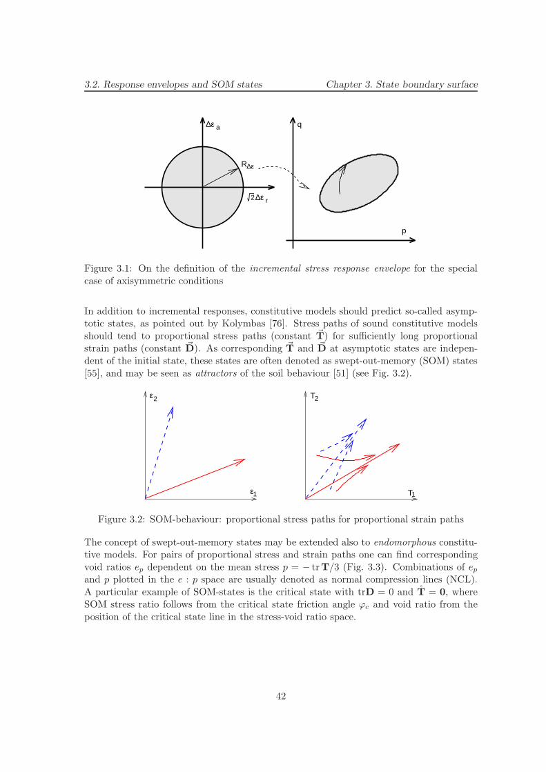
3.2. Response envelopes and SOM states Chapter 3. State boundary surface
∆ε r2
∆ε a q
p
R∆ε
Figure 3.1: On the definition of the incremental stress response envelope for the specialcase of axisymmetric conditions
In addition to incremental responses, constitutive models should predict so-called asymp-totic states, as pointed out by Kolymbas [76]. Stress paths of sound constitutive modelsshould tend to proportional stress paths (constant ~T) for sufficiently long proportionalstrain paths (constant ~D). As corresponding ~T and ~D at asymptotic states are indepen-dent of the initial state, these states are often denoted as swept-out-memory (SOM) states[55], and may be seen as attractors of the soil behaviour [51] (see Fig. 3.2).
ε
ε T
T
2
1 1
2
Figure 3.2: SOM-behaviour: proportional stress paths for proportional strain paths
The concept of swept-out-memory states may be extended also to endomorphous constitu-tive models. For pairs of proportional stress and strain paths one can find correspondingvoid ratios ep dependent on the mean stress p = − trT/3 (Fig. 3.3). Combinations of epand p plotted in the e : p space are usually denoted as normal compression lines (NCL).A particular example of SOM-states is the critical state with trD = 0 and T = 0, whereSOM stress ratio follows from the critical state friction angle ϕc and void ratio from theposition of the critical state line in the stress-void ratio space.
42
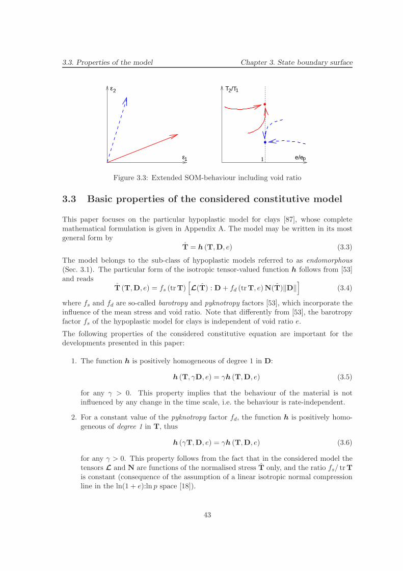
3.3. Properties of the model Chapter 3. State boundary surface
pe/eε
ε T2
1
2/T1
1
Figure 3.3: Extended SOM-behaviour including void ratio
3.3 Basic properties of the considered constitutive model
This paper focuses on the particular hypoplastic model for clays [87], whose completemathematical formulation is given in Appendix A. The model may be written in its mostgeneral form by
T = h (T,D, e) (3.3)
The model belongs to the sub-class of hypoplastic models referred to as endomorphous(Sec. 3.1). The particular form of the isotropic tensor-valued function h follows from [53]and reads
T (T,D, e) = fs (trT)[
L(T) : D + fd (trT, e)N(T)‖D‖]
(3.4)
where fs and fd are so-called barotropy and pyknotropy factors [53], which incorporate theinfluence of the mean stress and void ratio. Note that differently from [53], the barotropyfactor fs of the hypoplastic model for clays is independent of void ratio e.
The following properties of the considered constitutive equation are important for thedevelopments presented in this paper:
1. The function h is positively homogeneous of degree 1 in D:
h (T, γD, e) = γh (T,D, e) (3.5)
for any γ > 0. This property implies that the behaviour of the material is notinfluenced by any change in the time scale, i.e. the behaviour is rate-independent.
2. For a constant value of the pyknotropy factor fd, the function h is positively homo-geneous of degree 1 in T, thus
h (γT,D, e) = γh (T,D, e) (3.6)
for any γ > 0. This property follows from the fact that in the considered model thetensors L and N are functions of the normalised stress T only, and the ratio fs/ trTis constant (consequence of the assumption of a linear isotropic normal compressionline in the ln(1 + e):ln p space [18]).
43

3.4. Limit surface and Bounding surface Chapter 3. State boundary surface
For cases described by Eq. (3.6), the behaviour may be normalised by the currentmean stress p, or in a general case, by Hvorslev’s equivalent pressure on the isotropicnormal compression line p∗e. This procedure will be applied in Sec. 3.5.
3. The model predicts swept-out-memory states, introduced in Sec. 3.2. For a discussionon the prediction of SOM behaviour by hypoplastic models the reader is referred to[106].
Before proceeding to the derivation of the state boundary surface of the considered con-stitutive model, we recall some basic properties of more simple amorphous hypoplasticmodels.
3.4 Limit surface and Bounding surface
Amorphous hypoplastic constitutive models (e.g. model from [149]) may still be writtenusing Eq. (3.4) [80], considering fd = const. Eq. (3.3) therefore reduces to
T = h (T,D) (3.7)
For brevity, we will consider the factor fs in Eq. (3.4) embedded in the constitutive tensorsL and N. Therefore, we may write
T (T,D) = L(T) : D + N(T)‖D‖ (3.8)
Based on the fundamental experimental evidence, all reasonable constitutive models forsoils must consider the domain of admissible states in the stress space, bounded by a surface,formally defined through an isotropic tensor function. In the sequel, we will distinguishbetween two different notions: limit surface and bounding surface:
1. Limit surface [29] f(T), sometimes referred to as invertibility surface [133], failuresurface [154] or yield surface [77], is defined in the stress space as a boundary of allstates where Eq. (3.7) is invertible.
2. Bounding surface [106] b(T) (or bound surface [154]) is defined in the stress space asa boundary of all admissible states.1
Limit surface has been embedded even in very early versions of hypoplastic models (see,e.g., [76]) as a by-product of a particular choice of tensorial constitutive functions. It hasbeen however soon recognised that the mathematical structure of Eq. (3.8) allows us todefine the limit surface explicitly (e.g., [26, 9, 141]).
1Note that this definition is different compared to the one usually adopted for bounding surface plasticitymodels [38] and kinematic hardening elasto-plastic models (e.g., [127]), where the term bounding surface isused for the intersection of the state boundary surface and an elastic wall.
44
3.4. Limit surface and Bounding surface Chapter 3. State boundary surface
Following [133], Eq. (3.8) may be written as
γS = L : D + N‖D‖ (3.9)
with γ being the norm of the stress increment γ = ‖T‖ and S its direction S =~T. Due to
the Property 1. of Sec. 3.3 we may, without loss of generality, assume ‖D‖ = 1. Eq. (3.9)then reads
γS = L : ~D + N = L : (~D + B) (3.10)
withB = L
−1 : N (3.11)
Expressing (3.11) obviously requires invertibility of the tensor L of the particular amor-phous hypoplastic model.
From Eq. (3.10) we get~D = γL−1 : S− B (3.12)
Because ‖~D‖ = 1, we have1 = ‖γL−1 : S − B‖ (3.13)
and thereforeγ2‖L−1 : S‖2 − 2γ(L−1 : S) : B + ‖B‖2 − 1 = 0 (3.14)
For states inside the limit surface we require that Eq. (3.14) has a single real positivesolution for the norm of the stress increment γ. It may be shown from the requirement
(L−1 : S) : B <
√
[(L−1 : S) : B]2 − ‖L−1 : S‖2(‖B‖2 − 1) (3.15)
that this condition is satisfied for‖B‖2 − 1 < 0 (3.16)
Equation‖B‖2 − 1 = 0 (3.17)
therefore describes the limit of invertibility of Eq. (3.8) and, according to its definition,the limit surface2. The fact that one solution corresponds to γ = 0 may be representedgraphically using the concept of response envelopes (Sec. 3.2). As may be seen fromFig. 3.4, the reference stress point is then located on the response envelope. For statesoutside the limit surface the solution of Eq. (3.14) is not unique and the reference stresspoint is located outside the response envelope.
An investigation of Fig. 3.4 reveals that the limit surface f(T) does not coincide with thebounding surface b(T): for some directions of stretching the corresponding stress ratessurpass f(T). This fact, which was already described for example in [154], is a commonfeature of hypoplastic models developed at the University of Karlsruhe (see [133]) and is
2Eqs. (3.10)–(3.17) are useful for the subsequent comparison of the limit and bounding surfaces. Limitsurface may be also found directly from T = 0 following, e.g., [154]. In that case 0 = L : (D + B‖D‖),thus ~D = −B and ‖B‖ − 1 = 0 at the limit surface, which corresponds to (3.17).
45
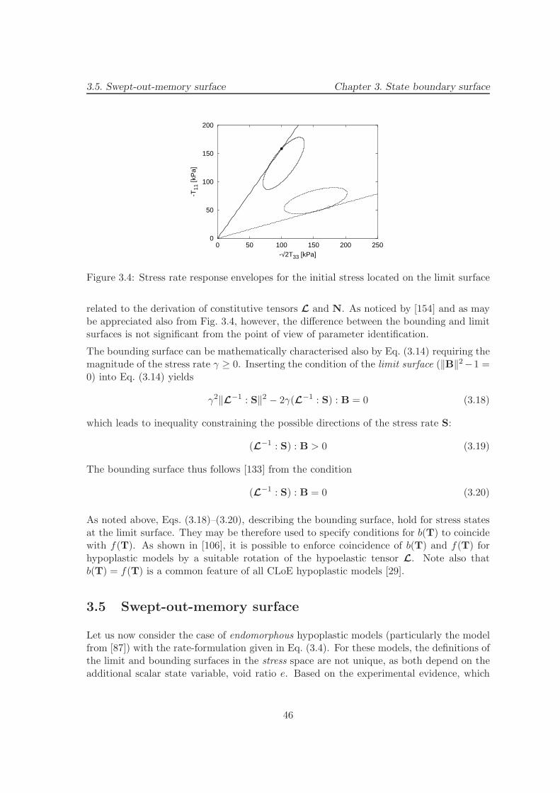
3.5. Swept-out-memory surface Chapter 3. State boundary surface
0
50
100
150
200
0 50 100 150 200 250
-T11
[kP
a]
-√2T33 [kPa]
Figure 3.4: Stress rate response envelopes for the initial stress located on the limit surface
related to the derivation of constitutive tensors L and N. As noticed by [154] and as maybe appreciated also from Fig. 3.4, however, the difference between the bounding and limitsurfaces is not significant from the point of view of parameter identification.
The bounding surface can be mathematically characterised also by Eq. (3.14) requiring themagnitude of the stress rate γ ≥ 0. Inserting the condition of the limit surface (‖B‖2−1 =0) into Eq. (3.14) yields
γ2‖L−1 : S‖2 − 2γ(L−1 : S) : B = 0 (3.18)
which leads to inequality constraining the possible directions of the stress rate S:
(L−1 : S) : B > 0 (3.19)
The bounding surface thus follows [133] from the condition
(L−1 : S) : B = 0 (3.20)
As noted above, Eqs. (3.18)–(3.20), describing the bounding surface, hold for stress statesat the limit surface. They may be therefore used to specify conditions for b(T) to coincidewith f(T). As shown in [106], it is possible to enforce coincidence of b(T) and f(T) forhypoplastic models by a suitable rotation of the hypoelastic tensor L. Note also thatb(T) = f(T) is a common feature of all CLoE hypoplastic models [29].
3.5 Swept-out-memory surface
Let us now consider the case of endomorphous hypoplastic models (particularly the modelfrom [87]) with the rate-formulation given in Eq. (3.4). For these models, the definitions ofthe limit and bounding surfaces in the stress space are not unique, as both depend on theadditional scalar state variable, void ratio e. Based on the experimental evidence, which
46

3.5. Swept-out-memory surface Chapter 3. State boundary surface
led in 1960’s to the development of the critical state soil mechanics in Cambridge [117, 122],the constitutive model should describe a single surface in the stress-void ratio space, whichbounds all admissible states. This surface is traditionally called state boundary surface(SBS). It is, in general, a surface in the four-dimensional space of the three principalcomponents of the stress tensor T and void ratio e.
The property 2. from Sec. 3.3 allows us to simplify the following developments by intro-ducing a normalisation factor taking into account both changes of void ratio and of meanpressure. A suitable quantity is Hvorslev’s equivalent pressure p∗e at the isotropic normalcompression line (see Fig. 3.5), following from the formulation of the isotropic NCL:
ln(1 + e) = N − λ∗ ln
(
p∗epr
)
(3.21)
with pr being the reference stress of 1 kPa. Using this normalisation the state boundary
pe*crp
*λ
*κ
Critical state line
ln p
ln (1+e)
Isotr. normal compression line
N
current stateIsotr. unloading line
1
1
Figure 3.5: On the definition of Hvorslev’s equivalent pressure p∗e.
surface may be, in general, fully characterised in the three-dimensional space defined bythe principal components of the normalised stress tensor Tn, where
Tn =T
p∗e(3.22)
The normalised stress rate Tn follows from (3.22)
Tn =T
p∗e− T
(p∗e)2 p
∗e (3.23)
The stress rate T is, under the assumption of small strains, given by (3.4) and the rate ofp∗e is found by the time-differentiation of the isotropic NCL given by Eq. (3.21):
e
1 + e= −λ
∗
p∗ep∗e (3.24)
47
3.5. Swept-out-memory surface Chapter 3. State boundary surface
From the assumption of grain incompressibility we have
e = (1 + e) tr D (3.25)
and thus
p∗e = − p∗e
λ∗trD (3.26)
Substituting (3.4) and (3.26) into (3.23) we get
Tn =1
p∗e(LD + fdN‖D‖) +
T trD
p∗eλ∗ (3.27)
For brevity, barotropy factor fs has been embedded in the constitutive tensors L and N.
We first try to find an expression equivalent to the limit surface in the stress-void ratiospace. As the limit surface in the stress space was defined by T = 0 for one direction ofstretching ~D (Eq. 3.17), we define its equivalent in the stress-void ratio space by Tn = 0.By applying this definition on (3.27) we get
−T
λ∗trD = L : D + fdN‖D‖ (3.28)
To solve Eq. (3.28) for a given T with unknowns ~D and fd, we introduce a fourth ordertensor A
A = L +1
λ∗T ⊗ 1 (3.29)
such that
A : ~D = L : ~D +T
λ∗tr ~D (3.30)
Eq. (3.28) may be divided by ‖D‖ 6= 0 and rewritten
A : ~D + fdN = 0 (3.31)
Since ‖~D‖ = 1, we getfd = ‖A−1 : N‖−1 (3.32)
(for invertibility condition of the tensor A see Appendix B) and
~D = − A−1 : N
‖A−1 : N‖(3.33)
As may be seen from the definitions of tensors A and N, the quantity A−1 : N, andtherefore also ~D and fd for Tn = 0, are constant for a given ~T. As the condition Tn = 0indeed implies ~T = const., Eq. (3.28) describes asymptotic (swept-out-memory) states asdefined in Sec. 3.2, provided that the evolution equation for fd is consistent with (3.28).Therefore, we name the equivalent of the limit surface for the stress-void ratio space aswept-out-memory (SOM) surface. From (3.28) it is also obvious that condition trD = 0directly implies T = 0, so the critical state is predicted as a particular SOM state.
48

3.6. State boundary surface Chapter 3. State boundary surface
The corresponding response in the p : e space may be found by taking the trace of Eq. (3.28)and considering L : D + fdN‖D‖ = T. We get
p = − p
λ∗tr D (3.34)
which is the rate formulation of the normal compression line with the slope λ∗ in theln(1 + e) : ln p space. Positions of different NCLs in this space (and therefore the shapeof the SOM surface) are controlled by the pyknotropy factor fd, which in the consideredmodel reads
fd =
(
2p
p∗e
)α
(3.35)
with α being a constant calculated from the model parameters (see Appendix A) and p∗ecomes from (3.21). Factor fd is constant along any line characterised by (3.34), whichensures consistency between evolution equation for fd and (3.28) and thus implies that Eq.(3.28) describes SOM states.
Combining Eqs. (3.32) and (3.35) allows us to calculate the value of p∗e at the SOM sur-face at any stress level T and consequently to find the shape of the SOM surface in thenormalised Tn space:
p∗e = − 2
3trT‖A−1 : N‖1/α (3.36)
The shape of the SOM surface in the normalised triaxial stress space, plotted for triaxialstress invariants q = −(Ta −Tr) and p, is shown in Fig. 3.6 for material parameters givenin Tab. 3.1.
-0.4
-0.2
0
0.2
0.4
0 0.2 0.4 0.6 0.8 1
q/p* e
p/p*e
critical stateK0NC conditions
Figure 3.6: Swept-out-memory surface in the normalised triaxial stress space for the hy-poplastic model [87] using London clay parameters (Tab. 3.1)
3.6 State boundary surface
In this section we discuss the difference between the swept-out-memory surface, definedin Sec. 3.5, and the state boundary surface. Without loss of generality we again study
49

3.6. State boundary surface Chapter 3. State boundary surface
response of the considered model in the normalised space Tn. The state boundary surfaceis defined as an envelope of all admissible states of a soil element. In other words, no outerresponse in the normalised space Tn can be generated. Using the concept of responseenvelopes (Sec. 3.2), stress rate response envelope plotted in the normalised Tn space(normalised response envelope, NRE) for the states at the state boundary surface mustnot cross-sect the surface (i.e., must have a common tangent with the state boundarysurface).
We first presume that the state boundary surface is equal to the swept-out-memory surface.A tangent to the normalised response envelope may then be found using a similar procedureto that applied in Sec. 3.4 for evaluation of bounding surface of amorphous hypoplasticmodels. Let γn be the norm of the normalised stress rate Tn (γn = ‖Tn‖) and Sn itsdirection (Sn = Tn/‖Tn‖). Using the definition of the tensor A (Eq. 3.29) and assuming,without loss of generality, ‖D‖ = 1, Eq. (3.27) reads
p∗eγnSn = A : ~D + fdN (3.37)
orp∗eγnSn = A : (~D + fdBn) (3.38)
withBn = A
−1 : N (3.39)
Thus (from (3.38))~D = p∗eγnA
−1 : Sn − fdBn (3.40)
taking the norm of (3.40) we get
(p∗e)2γ2n‖A−1 : Sn‖2 − 2p∗eγnfd
(
A−1 : Sn
)
: Bn + f2d‖Bn‖2 − 1 = 0 (3.41)
For the states at the SOM surface we have fd = ‖Bn‖−1 (3.32). Introducing this conditioninto (3.41) leads to
p∗eγ2n‖A−1 : Sn‖2 − 2γn
(
A−1 : Sn
)
: ~DSOM = 0 (3.42)
where ~DSOM is the direction of the proportional stretching corresponding to the swept-out-memory conditions for a given state Tn (from 3.33):
~DSOM = − Bn
‖Bn‖(3.43)
As γn represents the norm of Tn, it must be positive or null. Therefore, possible directionsSn must be confined in the half-space defined by
(
A−1 : Sn
)
: ~DSOM > 0 (3.44)
where the plane(
A−1 : Sn
)
: ~DSOM = 0 (3.45)
50

3.6. State boundary surface Chapter 3. State boundary surface
-0.4
-0.2
0
0.2
0.4
0 0.2 0.4 0.6 0.8 1
q/p* e
p/p*e
SOM surfaceNIREs
tangent to NRE
(a)
0.33
0.332
0.334
0.336
0.338
0.34
0.342
0.344
0.346
0.348
0.35
0.87 0.875 0.88 0.885 0.89
q/p* e
p/p*e
SOM surfaceNIRE, R∆ε=0.001
tangent to NRE
(b)
Figure 3.7: NIREs for the initial K0NC conditions. (b) provides detail of (a). NIREs areplotted for R∆ǫ = 0.001, 0.0025, 0.005, 0.01, 0.02 (a) and R∆ǫ = 0.001 (b). Points atNIREs denote compression and extension for D00 = D11 = D22 and trD = 0)
represents a tangent to the normalised response envelope.
Fig. 3.7a depicts the SOM surface, tangent to the normalised response envelope calculatedaccording to Eq. (3.45) and incremental stress response envelopes (as defined in Sec. 3.2)plotted in the normalised space Tn (normalised incremental response envelope, NIRE) fordifferent values of R∆ǫ. Apparently, the tangent to the normalised response envelope isnearly coincident with the tangent to the SOM surface. A detailed inspection in Fig. 3.7b,however, reveals that the tangent to the NRE is slightly inclined with respect to the tangentto the SOM surface and therefore proves that the state boundary surface, in general, doesnot coincide with the swept-out-memory surface. The difference between tangents to NREand SOM surface is even more pronounced for initial states dry of critical (defined byp/p∗e < 0.5 in the model considered) as shown in Fig. 3.83.
Therefore, similarly to the limit and bounding surfaces of amorphous hypoplastic modelsin the stress space, the state boundary surface is located slightly outside the swept-out-memory surface. Nevertheless, taking into account uncertainties in the experimental de-termination of the state boundary surface, we may consider the swept-out-memory surfaceas a sufficient approximation of the state boundary surface. For this reason we restrict ourinvestigations in the next sections to the SOM surface.
Figures 3.7 and 3.8 also demonstrate the asymptotic property of the considered hypoplasticmodel, as for large R∆ǫ the normalised incremental response envelopes converge towardsthe SOM surface. The model keeps this property also for the initial states outside theSOM surface (see Fig. 3.9). Therefore, we see that the fact that the model allows tosurpass slightly the SOM surface (SBS is located slightly outside the SOM surface) does
3In Fig. 3.8 normalised incremental response envelopes are cross-sected by the tangent to normalisedresponse envelopes calculated according to (3.45). This fact is to be expected, as, in general, a tangent tothe NRE represents a tangent to the NIRE only for R∆ǫ → 0.
51
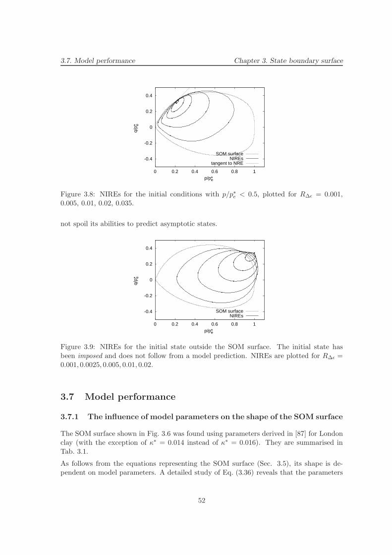
3.7. Model performance Chapter 3. State boundary surface
-0.4
-0.2
0
0.2
0.4
0 0.2 0.4 0.6 0.8 1
q/p* e
p/p*e
SOM surfaceNIREs
tangent to NRE
Figure 3.8: NIREs for the initial conditions with p/p∗e < 0.5, plotted for R∆ǫ = 0.001,0.005, 0.01, 0.02, 0.035.
not spoil its abilities to predict asymptotic states.
-0.4
-0.2
0
0.2
0.4
0 0.2 0.4 0.6 0.8 1
q/p* e
p/p*e
SOM surfaceNIREs
Figure 3.9: NIREs for the initial state outside the SOM surface. The initial state hasbeen imposed and does not follow from a model prediction. NIREs are plotted for R∆ǫ =0.001, 0.0025, 0.005, 0.01, 0.02.
3.7 Model performance
3.7.1 The influence of model parameters on the shape of the SOM surface
The SOM surface shown in Fig. 3.6 was found using parameters derived in [87] for Londonclay (with the exception of κ∗ = 0.014 instead of κ∗ = 0.016). They are summarised inTab. 3.1.
As follows from the equations representing the SOM surface (Sec. 3.5), its shape is de-pendent on model parameters. A detailed study of Eq. (3.36) reveals that the parameters
52
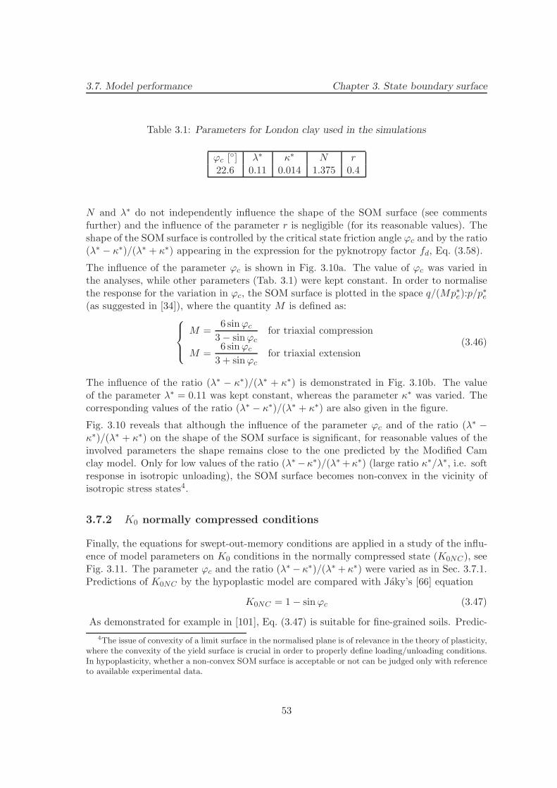
3.7. Model performance Chapter 3. State boundary surface
Table 3.1: Parameters for London clay used in the simulations
ϕc [◦] λ∗ κ∗ N r22.6 0.11 0.014 1.375 0.4
N and λ∗ do not independently influence the shape of the SOM surface (see commentsfurther) and the influence of the parameter r is negligible (for its reasonable values). Theshape of the SOM surface is controlled by the critical state friction angle ϕc and by the ratio(λ∗ − κ∗)/(λ∗ + κ∗) appearing in the expression for the pyknotropy factor fd, Eq. (3.58).
The influence of the parameter ϕc is shown in Fig. 3.10a. The value of ϕc was varied inthe analyses, while other parameters (Tab. 3.1) were kept constant. In order to normalisethe response for the variation in ϕc, the SOM surface is plotted in the space q/(Mp∗e):p/p
∗e
(as suggested in [34]), where the quantity M is defined as:
M =6 sinϕc
3 − sinϕcfor triaxial compression
M =6 sinϕc
3 + sinϕcfor triaxial extension
(3.46)
The influence of the ratio (λ∗ − κ∗)/(λ∗ + κ∗) is demonstrated in Fig. 3.10b. The valueof the parameter λ∗ = 0.11 was kept constant, whereas the parameter κ∗ was varied. Thecorresponding values of the ratio (λ∗ − κ∗)/(λ∗ + κ∗) are also given in the figure.
Fig. 3.10 reveals that although the influence of the parameter ϕc and of the ratio (λ∗ −κ∗)/(λ∗ + κ∗) on the shape of the SOM surface is significant, for reasonable values of theinvolved parameters the shape remains close to the one predicted by the Modified Camclay model. Only for low values of the ratio (λ∗−κ∗)/(λ∗ +κ∗) (large ratio κ∗/λ∗, i.e. softresponse in isotropic unloading), the SOM surface becomes non-convex in the vicinity ofisotropic stress states4.
3.7.2 K0 normally compressed conditions
Finally, the equations for swept-out-memory conditions are applied in a study of the influ-ence of model parameters on K0 conditions in the normally compressed state (K0NC), seeFig. 3.11. The parameter ϕc and the ratio (λ∗ − κ∗)/(λ∗ + κ∗) were varied as in Sec. 3.7.1.Predictions of K0NC by the hypoplastic model are compared with Jaky’s [66] equation
K0NC = 1 − sinϕc (3.47)
As demonstrated for example in [101], Eq. (3.47) is suitable for fine-grained soils. Predic-
4The issue of convexity of a limit surface in the normalised plane is of relevance in the theory of plasticity,where the convexity of the yield surface is crucial in order to properly define loading/unloading conditions.In hypoplasticity, whether a non-convex SOM surface is acceptable or not can be judged only with referenceto available experimental data.
53

3.8. Concluding remarks Chapter 3. State boundary surface
-0.6
-0.4
-0.2
0
0.2
0.4
0.6
0 0.2 0.4 0.6 0.8 1
q/(M
p* e)
p/p*e
ϕc=15°ϕc=20°
ϕc=22.6°ϕc=25°ϕc=30°
(a)
-0.4
-0.2
0
0.2
0.4
0 0.2 0.4 0.6 0.8 1
q/p* e
p/p*e
κ*=0.002, rat.=0.964κ*=0.006, rat.=0.897κ*=0.010, rat.=0.833κ*=0.014, rat.=0.774κ*=0.018, rat.=0.719κ*=0.022, rat.=0.667
(b)
Figure 3.10: The influence of (a) the parameter ϕc and (b) of the ratio (λ∗ −κ∗)/(λ∗ +κ∗)on the shape of the SOM surface
tions by the Modified Cam clay model [117] are also included in Fig. 3.11. In the calculationwith the Modified Cam clay model, the influence of elastic strain increments, which are atthe yield surface negligible compared to the plastic strain increments, is omitted. Conse-quently,
K0NC =3 − η
3 + 2η(3.48)
for the Modified Cam clay model, with
η =
√9 + 4M2 − 3
2and M =
6 sinϕc3 − sinϕc
(3.49)
It can be seen in Fig. 3.11 that the considered hypoplastic model predicts correctly thetrend of decreasing K0NC with increasing ϕc. Although the hypoplastic model overpredictsK0NC as compared to Eq. (3.47), its predictions are still significantly closer to Eq. (3.47)than the predictions by the Modified Cam clay model.
Further discussion on the direction of stretching ~D at SOM conditions with respect to thecorresponding ~T, as well as on the SOM conditions predicted by different endomorphoushypoplastic models, may be found in [96].
3.8 Concluding remarks
The present paper studied if the hypoplastic model for clays [87] predicts, as a by–productof the constitutive formulation, the existence of the state boundary surface, which may beseen as a key characteristics of the behaviour of fine–grained soils.
It has been shown that for the given model it is possible to derive an explicit formulation forthe so-called swept-out-memory surface, which may be defined as an envelope of asymptotic
54

3.8. Concluding remarks Chapter 3. State boundary surface
0.5
0.55
0.6
0.65
0.7
0.75
0.8
0.85
0.9
0.95
14 16 18 20 22 24 26 28 30
K0N
C
ϕc°
clay hypoplas., rat.=0.774Mod. Cam clay
1-sinϕc
(a)
0.5
0.55
0.6
0.65
0.7
0.75
0.8
0.85
0.65 0.7 0.75 0.8 0.85 0.9 0.95 1
K0N
C
ratio (λ*-κ*)/(λ*+κ*)
clay hypoplas., ϕc=22.6°Mod. Cam clay, ϕc=22.6°
1-sinϕc
(b)
Figure 3.11: K0NC conditions predicted by the considered model, compared to Jaky’s [66]formula and predictions by the Modified Cam clay model [117].
(swept-out-memory) states in the stress-void ratio space. The concept of the normalisedincremental stress response envelopes and the derivation of the tangent to the normalisedrate response envelopes was subsequently used to demonstrate that the swept-out-memorysurface is a close approximation of the state boundary surface, although, in general, theydo not coincide. It has been shown that there is a direct parallel between the swept-out-memory and the state boundary surfaces defined in the stress-void ratio space forendomorphous hypoplastic models, and limit and bounding surfaces defined in the stressspace for amorphous hypoplastic models.
Finally the influence of the constitutive parameters on the shape of the swept-out-memorysurface has been studied by means of a parametric study. For parameters suitable forfine-grained soils, the considered hypoplastic model predicts a swept-out-memory surfaceof a similar shape to the state boundary surface of the Modified Cam clay model. However,the K0 values at normally compressed states are better predicted by the hypoplastic modelthan by the Modified Cam clay model.
A study of the shape of the SOM surface (Sec. 3.7) and invertibility condition of A (Ap-pendix B) reveal limitation of the hypoplastic model for clays, which does not perform cor-rectly for soils very soft in isotropic unloading. As a very rough guide, condition κ∗ < λ∗/4should be satisfied when using model [87]. More precise investigation requires to plot theSOM surface and to ensure that the condition (3.66) is not satisfied.
Appendix A
The mathematical structure of the hypoplastic model for clays is discussed in detail in [87].The constitutive equation in rate form reads:
T = fsL : D + fsfdN‖D‖ (3.50)
55

3.8. Concluding remarks Chapter 3. State boundary surface
where:
L = 3(
c1I + c2a2T ⊗ T
)
N = L :
(
−Y m
‖m‖
)
T :=T
trT(3.51)
1 is the second–order identity tensor and I is the fourth–order identity tensor, with com-ponents:
(I)ijkl :=1
2(1ik1jl + 1il1jk) (3.52)
In eq. (3.50), the functions fs(tr T) (barotropy factor) and fd(trT, e) (pyknotropy factor)are given by:
fs = − trT
λ∗
(
3 + a2 − 2αa√
3)−1
fd =
[
− 2trT
3prexp
(
ln (1 + e) −N
λ∗
)]α
(3.53)
where pr is the reference stress 1 kPa. The scalar function Y and the second–order tensorm appearing in Eq. (3.51) are given, respectively, by:
Y =
( √3a
3 + a2− 1
)
(I1I2 + 9I3)(
1 − sin2 ϕc)
8I3 sin2 ϕc+
√3a
3 + a2(3.54)
in which:
I1 := trT I2 :=1
2
[
T : T− (I1)2]
I3 := detT
and
m = − a
F
[
T + T∗ − T
3
(
6 T : T − 1
(F/a)2 + T : T
)]
(3.55)
in which:
T∗
= T − 1
3F =
√
1
8tan2 ψ +
2 − tan2 ψ
2 +√
2 tanψ cos 3θ− 1
2√
2tanψ (3.56)
tanψ =√
3‖T∗‖ cos 3θ = −√
6tr(
T∗ · T∗ · T∗)
(
T∗
: T∗)3/2
(3.57)
Finally, the scalars a, α, c1 and c2 appearing in eqs. (3.51)–(3.55), are given as functionsof the material parameters ϕc, λ
∗, κ∗ and r by the following relations:
a =
√3 (3 − sinϕc)
2√
2 sinϕcα =
1
ln 2ln
[
λ∗ − κ∗
λ∗ + κ∗
(
3 + a2
a√
3
)]
(3.58)
c1 =2(
3 + a2 − 2αa√
3)
9rc2 = 1 + (1 − c1)
3
a2(3.59)
The model requires five constitutive parameters, namely ϕc, λ∗, κ∗, N and r, state is
characterised by the Cauchy stress T and void ratio e.
56
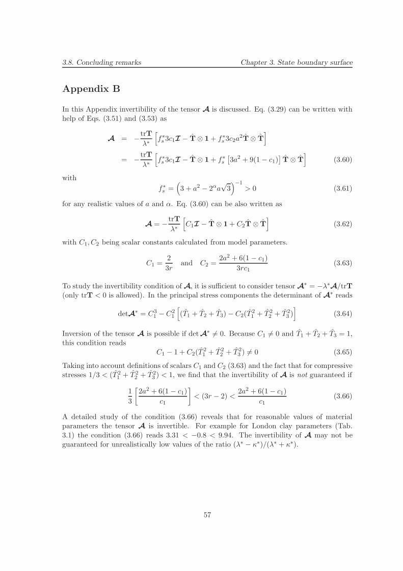
3.8. Concluding remarks Chapter 3. State boundary surface
Appendix B
In this Appendix invertibility of the tensor A is discussed. Eq. (3.29) can be written withhelp of Eqs. (3.51) and (3.53) as
A = −trT
λ∗
[
f∗s 3c1I − T ⊗ 1 + f∗s 3c2a2T⊗ T
]
= −trT
λ∗
[
f∗s 3c1I − T ⊗ 1 + f∗s[
3a2 + 9(1 − c1)]
T ⊗ T]
(3.60)
with
f∗s =(
3 + a2 − 2αa√
3)−1
> 0 (3.61)
for any realistic values of a and α. Eq. (3.60) can be also written as
A = −trT
λ∗
[
C1I − T ⊗ 1 + C2T ⊗ T]
(3.62)
with C1, C2 being scalar constants calculated from model parameters.
C1 =2
3rand C2 =
2a2 + 6(1 − c1)
3rc1(3.63)
To study the invertibility condition of A, it is sufficient to consider tensor A∗ = −λ∗A/trT
(only trT < 0 is allowed). In the principal stress components the determinant of A∗ reads
detA∗ = C31 − C2
1
[
(T1 + T2 + T3) − C2(T21 + T 2
2 + T 23 )]
(3.64)
Inversion of the tensor A is possible if det A∗ 6= 0. Because C1 6= 0 and T1 + T2 + T3 = 1,this condition reads
C1 − 1 + C2(T21 + T 2
2 + T 23 ) 6= 0 (3.65)
Taking into account definitions of scalars C1 and C2 (3.63) and the fact that for compressivestresses 1/3 < (T 2
1 + T 22 + T 2
3 ) < 1, we find that the invertibility of A is not guaranteed if
1
3
[
2a2 + 6(1 − c1)
c1
]
< (3r − 2) <2a2 + 6(1 − c1)
c1(3.66)
A detailed study of the condition (3.66) reveals that for reasonable values of materialparameters the tensor A is invertible. For example for London clay parameters (Tab.3.1) the condition (3.66) reads 3.31 < −0.8 < 9.94. The invertibility of A may not beguaranteed for unrealistically low values of the ratio (λ∗ − κ∗)/(λ∗ + κ∗).
57

Chapter 4
Directional response of areconstituted fine-grained soil:Performance of differentconstitutive models
4.1 Introduction
The directional character of the mechanical response of fine-grained soils, i.e., its depen-dence on the loading direction, has been the subject of several studies throughout the lastdecades, including both experimental and theoretical investigations. On the experimentalside, some pioneering contributions were provided in the early seventies, see e.g., Refer-ences [81, 147]. Notable examples of more recent contributions can be found in the worksof Graham et al. [48], Atkinson et al. [6], Smith et al. [123] and Callisto and Calabresi[20]. On the theoretical side, a major improvement of classical plasticity as applied to clayshas been provided by the introduction of the so-called nested-surface kinematic hardeningtheories of plasticity, originating from the works of Prevost [113], Mroz et al. [102] andHashiguchi [57]. These latter studies were essentially motivated by the need of improvingavailable design approaches for those practical applications where soil is subject to cyclicloading conditions, e.g., earthquakes, offshore engineering, etc.
Later studies on shear banding in soils as a bifurcation problem [121, 115] showed the needto take into account the incrementally non-linear character of the material response – i.e.,a dependence of soil tangent stiffness on the strain rate direction, see, e.g., References[39, 132] – and motivated the development of a class of constitutive theories which departfrom the framework of plasticity and rather can be seen as a generalization of Truesdelltheory of hypoelasticity [137]. A distinctive feature of this approach is the absence of anykinematic decomposition of strain rates into reversible and irreversible parts. An importantexample in this respect is provided by the theory of hypoplasticity, as defined by Kolymbas
58

4.1. Introduction Chapter 4. Directional response
[77], see also Reference [80].
More generally, it turns out that a proper description of soil behavior as a function ofloading direction not only is useful for modelling the response of geotechnical structuresto cyclic loading or for analyzing localization phenomena, but it is also a key ingredient inthe analysis of any geotechnical structure where different zones of soil experience widelydifferent stress-paths, both in size and direction, e.g., deep excavations and tunnels. Thishas been demonstrated in a number of practical applications, see, e.g. References [124, 146,45, 140].
The objective of this work is to assess, both qualitatively and quantitatively, the perfor-mance of some advanced constitutive models in reproducing the stress-strain behavior ofa soft, normally consolidated reconstituted clay as observed in laboratory tests performedalong a number of different stress-paths originating from a common initial state. Two par-ticular classes of inelastic models have been selected for the comparison. On the one hand,the three-surface kinematic hardening model proposed by Stallebrass [125]; Stallebrassand Taylor [127] has been chosen as the representative candidate of modern soil plasticityapproaches. On the other hand, three different versions of hypoplasticity have been con-sidered, which differ from each other in terms of history-related state variables, namely theCLoE model [29], the clay K-hypoplastic model recently proposed by Masın [87], and amodified version of this last model, embedding the concept of intergranular strain [108] asadditional internal state variable. Finally, the classical critical-state Modified Cam-Claymodel with associative flow rule [117] has been also considered as a reference.
The companion paper by Costanzo et al. [31] presents the results of a large program ofstress-probing tests on normally consolidated, reconstituted Beaucaire Marl. These resultsare used herein both for the calibration of the different models, and as a benchmark forthe evaluation of the models performance. The results obtained from standard isotropic ortriaxial compression and extension tests, starting from an isotropic state, were used for thecalibration of the different models. The assessment of models’ performance was carried outwith reference to a different set of data, obtained from axisymmetric stress-probing testsstarting from an anisotropic initial stress state.
The outline of the paper is as follows. The details of the experimental program are shortlyrecalled in Sect. 4.2. A summary of the main features of the constitutive models consideredis provided in Sect. 4.3. The procedures adopted for the calibration of the different modelsare thoroughly discussed in Sect. 4.4, before presenting the comparison between predictedand observed directional response, in Sect. 4.5, where a quantitative assessment of theperformance of the models is attempted by introducing suitable scalar measures of theprediction error. Finally, some concluding remarks are drawn and perspectives for furtherresearch are provided in Sect. 4.6.
In the following, the usual sign convention of soil mechanics (compression positive) isadopted throughout. In line with Terzaghi’s principle of effective stress, all stresses areeffective stresses, unless otherwise stated. Both direct and index notation will be used torepresent tensor quantities, according to convenience. Calligraphic letters are used to rep-resent fourth-order tensors and their components (e.g., L and Lijkl). In the representation
59

4.2. Experimental data Chapter 4. Directional response
of stress and strain states, use is sometimes made of the following invariant quantities:p := (1/3) tr σ (mean stress); q :=
√
(3/2) ‖dev(σ)‖ (deviatoric stress); ǫv := tr ǫ (volu-metric strain); and ǫs :=
√
(2/3) ‖dev(ǫ)‖ (deviatoric stress).
4.2 Experimental data from stress-probing tests
The material tested is a low plasticity silty clay, with a liquid limit of 38%, and a plas-ticity index of 17%. The stress-probing tests were performed on reconstituted material,consolidated in a large consolidometer up to a nominal vertical effective stress of 75 kPa.Full details of the experimental procedures employed in the testing program are given byCostanzo et al. [31]. Overall, the measurement system is capable of resolving strains ofapproximately 0.0005.
The testing program consisted of a large number of drained stress probes, starting from acommon initial stress state and pointing in different directions in the triaxial plane. Twodifferent initial stress states were considered: the first one (state A) is located on theisotropic axis at p = 150 kPa; the second one (state B) is characterized by the same meanstress as state A and a deviator stress q = 60 kPa. Both states A and B were reached uponstress-controlled consolidation along a constant q/p path (q/p = 0 for state A, q/p = 0.4for state B). Each stress probe from an initial state (σa0, σr0) is described by the followingparametric equations:
∆σa := σa − σa0 = Rσ sinασ (4.1)√
2 ∆σr :=√
2σr − σr0 = Rσ cosασ (4.2)
where Rσ = ‖∆σ‖ denotes the norm of the stress increment, and ασ represents its directionin the Rendulic plane of stress increments (∆σa :
√2∆σr, see Fig. 4.1a). Each stress probe
was continued up to a Rσ value corresponding either to a ”failure” state, or to a prescribedmaximum value of the cell pressure. The loading directions ασ prescribed for each probeare listed in Tab. 4.1. Note that for each initial state the testing program included asparticular cases conventional triaxial, constant p and isotropic, compression and extensionpaths. The stress probe direction in the q : p plane, αpqσ , calculated from the stress invariantincrements ∆ p and ∆ q as:
∆ p =1
3(∆σa + 2∆σr) ∆ q = ∆σa − ∆σr (4.3)
sinαpqσ =∆ q
√
(∆ p)2 + (∆ q)2cosαpqσ =
∆ p√
(∆ p)2 + (∆ q)2(4.4)
is also reported in the same table. A picture of the stress paths originating from initialstate B in the q : p plane is shown in Fig. 4.2.
60

4.2. Experimental data Chapter 4. Directional response
Dsa
Dsr2
Rs
Dea
Der2a
s
Re
ae
(a) (b)
Figure 4.1: Response envelope concept: a) input stress probes; b) output strain envelope.
Test Initial ασ αpqσ Test Initial ασ αpqσ# state (deg.) (deg.) # state (deg.) (deg.)
Tx124 A 0 303.69 Tx118 B 0 303.69Tx128 A 35 0.00 Tx115 B 35 0.00
— — — — Tx130 B 46 21.91Tx121 A 90 71.57 Tx132 B 90 71.57Tx126 A 126 90.00 Tx119 B 126 90.00
— — — — Tx116 B 154 104.49Tx123 A 180 123.69 — — — —Tx127 A 215 180.00 Tx134 B 215 180.00
— — — — Tx129 B 226 201.91Tx122 A 270 251.57 Tx117 B 270 251.57Tx125 A 305 270.00 Tx113 B 305 270.00
Table 4.1: Details of the experimental stress-probing program, after Costanzo et al. [31].
61
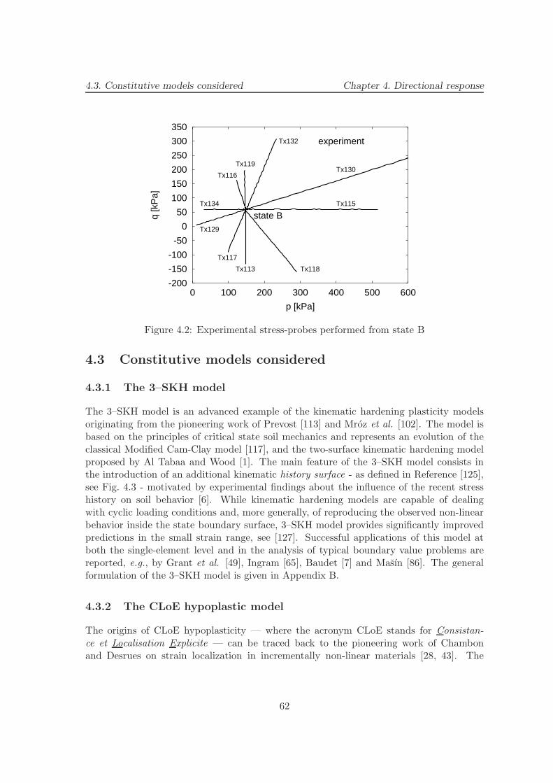
4.3. Constitutive models considered Chapter 4. Directional response
-200
-150
-100
-50
0
50
100
150
200
250
300
350
0 100 200 300 400 500 600
q [k
Pa]
p [kPa]
experiment
state BTx115
Tx130
Tx132
Tx119
Tx113 Tx118
Tx117
Tx116
Tx129
Tx134
Figure 4.2: Experimental stress-probes performed from state B
4.3 Constitutive models considered
4.3.1 The 3–SKH model
The 3–SKH model is an advanced example of the kinematic hardening plasticity modelsoriginating from the pioneering work of Prevost [113] and Mroz et al. [102]. The model isbased on the principles of critical state soil mechanics and represents an evolution of theclassical Modified Cam-Clay model [117], and the two-surface kinematic hardening modelproposed by Al Tabaa and Wood [1]. The main feature of the 3–SKH model consists inthe introduction of an additional kinematic history surface - as defined in Reference [125],see Fig. 4.3 - motivated by experimental findings about the influence of the recent stresshistory on soil behavior [6]. While kinematic hardening models are capable of dealingwith cyclic loading conditions and, more generally, of reproducing the observed non-linearbehavior inside the state boundary surface, 3–SKH model provides significantly improvedpredictions in the small strain range, see [127]. Successful applications of this model atboth the single-element level and in the analysis of typical boundary value problems arereported, e.g., by Grant et al. [49], Ingram [65], Baudet [7] and Masın [86]. The generalformulation of the 3–SKH model is given in Appendix B.
4.3.2 The CLoE hypoplastic model
The origins of CLoE hypoplasticity — where the acronym CLoE stands for Consistan-ce et Localisation Explicite — can be traced back to the pioneering work of Chambonand Desrues on strain localization in incrementally non-linear materials [28, 43]. The
62
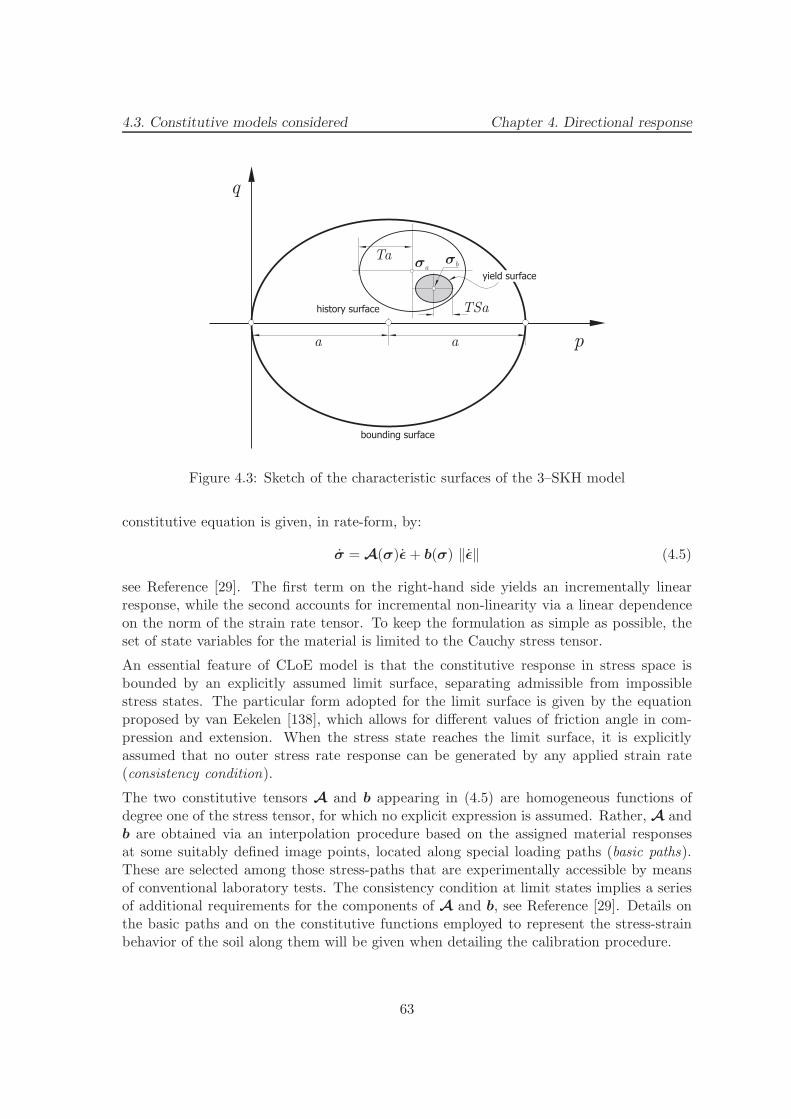
4.3. Constitutive models considered Chapter 4. Directional response
sasb
aa p
q
Ta
TSa
bounding surface
history surface
yield surface
Figure 4.3: Sketch of the characteristic surfaces of the 3–SKH model
constitutive equation is given, in rate-form, by:
σ = A(σ)ǫ + b(σ) ‖ǫ‖ (4.5)
see Reference [29]. The first term on the right-hand side yields an incrementally linearresponse, while the second accounts for incremental non-linearity via a linear dependenceon the norm of the strain rate tensor. To keep the formulation as simple as possible, theset of state variables for the material is limited to the Cauchy stress tensor.
An essential feature of CLoE model is that the constitutive response in stress space isbounded by an explicitly assumed limit surface, separating admissible from impossiblestress states. The particular form adopted for the limit surface is given by the equationproposed by van Eekelen [138], which allows for different values of friction angle in com-pression and extension. When the stress state reaches the limit surface, it is explicitlyassumed that no outer stress rate response can be generated by any applied strain rate(consistency condition).
The two constitutive tensors A and b appearing in (4.5) are homogeneous functions ofdegree one of the stress tensor, for which no explicit expression is assumed. Rather, A andb are obtained via an interpolation procedure based on the assigned material responsesat some suitably defined image points, located along special loading paths (basic paths).These are selected among those stress-paths that are experimentally accessible by meansof conventional laboratory tests. The consistency condition at limit states implies a seriesof additional requirements for the components of A and b, see Reference [29]. Details onthe basic paths and on the constitutive functions employed to represent the stress-strainbehavior of the soil along them will be given when detailing the calibration procedure.
63

4.3. Constitutive models considered Chapter 4. Directional response
4.3.3 The K-hypoplastic model for clays
The K-hypoplastic model considered in the present study has been recently developed byMasın [87] with the specific aim of describing the behavior of fine-grained soils. The modelcombines the mathematical structure of K-hypoplastic models – see e.g., Reference [153]and references therein – with key concepts of critical state soil mechanics [122] through thenotion of generalised hypoplasticity, as defined by Niemunis [106]. In fact, the model canbe considered an evolution of both von Wolffersdorff [141] model for sands, and the morerecent Herle and Kolymbas [61] model for soils with low friction angles
The constitutive equation is given, in rate-form, by:
σ = fsL : ǫ + fsfdN ‖ǫ‖ (4.6)
Explicit, closed form expressions for the two tensors L(σ) and N (σ) and for the scalarfunctions fs(p) and fd(p, e) are provided in Appendix B. It must be noted that, althoughEq. (4.6) and (4.5) appear quite similar, a major difference of K-hypoplasticity as comparedto CLoE stems from including void ratio in the set of state variables for the materialthrough the so-called pyknotropy factor fd [53]. It is precisely this ingredient which allowsthe critical state concept to be incorporated in the constitutive equation. A more generalcomparison between the two frameworks of CLoE- and K-hypoplasticity can be found inReference [133].
4.3.4 The K-hypoplastic model for clays with intergranular strain
The K-hypoplastic model discussed in the previous section is capable of predicting thebehavior of fine-grained soils upon monotonic loading at medium to large strain levels. Inorder to prevent excessive ratcheting upon cyclic loading and to improve model perfor-mance in the small-strain range, its mathematical formulation has been enhanced by theintergranular strain concept [108].
The mathematical formulation of this enhanced version of the K-hypoplastic model forclays is given by:
σ = M (σ, e, δ,η) : ǫ (4.7)
where M is the fourth-order tangent stiffness tensor of the material, η := ǫ/ ‖ǫ‖ denotesthe strain rate direction, and the additional state variable δ is a symmetric second ordertensor called intergranular strain. Full details of the mathematical structure of the modelare provided in appendix B.
In this formulation, the total strain can be thought of as the sum of a component relatedto the deformation of interface layers at integranular contacts, quantified by δ, and acomponent related to the rearrangement of the soil skeleton. For reverse loading conditions(η : δ < 0, where δ is defined in Appendix B) and neutral loading conditions (η : δ = 0), theobserved overall strain is related only to the deformation of the intergranular interface layerand the soil behaviour is hypoelastic, whereas in continued loading conditions (η : δ > 0)the observed overall response is also affected by particle rearrangement in the soil skeleton.
64

4.4. Model calibration Chapter 4. Directional response
From a mathematical standpoint, the response of the model is determined by interpolatingbetween the following three special cases:
σ = mRfsL : ǫ (η : δ = −1 ∧ δ = 0) (4.8)
σ = mT fsL : ǫ (η : δ = 0) (4.9)
σ = fsL : ǫ + fsfdN ‖ǫ‖ (η : δ = 1) (4.10)
the last case corresponding to the so-called swept-out-memory conditions [55]. The quan-tities mR and mT appearing in Eqs. 4.8 and 4.9 are material constants. The particularstructure adopted for the constitutive tensor L [87] should allow, in principle, to get agood performance in both the very small and large strain ranges.
4.4 Model calibration
When comparing the performance of different constitutive models in predicting the ob-served directional response of the material, particular care must be taken in the properselection of the procedure adopted for their calibration. In the present case, this task issomewhat made easier by the fact that all the constitutive models discussed in the previ-ous section, with the only exception of the CLoE hypoplastic model, incorporate the basicprinciples of Critical State Soil Mechanics, and thus some of the material constants sharethe same physical meaning.
In order to separate the data used for the calibration of the five models considered and thedata used for the evaluation of their performance, the material constants of each modelhave been determined from the results of the stress probes starting from the isotropic initialstate A. This is also consistent with the procedure typically used in practical applications,where most of the experimental data provided by the site investigation refer to isotropicallyconsolidated, drained or undrained triaxial tests.
For some of the constitutive models considered, the available data from stress probes atpoint A do not provide enough information to calibrate all the relevant constants. This isthe case, for example, of the material parameters controlling the response of the 3–SKH orK-hypoplastic models upon load reversal in the very small strain range. In such cases, thechoice has been made to evaluate such material constants based on the experience gatheredin previous experimental investigations on similar soils. Although such a choice necessarilyintroduces a certain degree of subjectivity in the comparative evaluation of the modelresponses, it can still be considered acceptable for our purposes, considering that the typicalrange of variation of such parameters for different soils is relatively limited, and the modelresponse is not very sensitive to their variation, see e.g., References [108, 125, 65, 30, 86].
It is important to note that, although the initial conditions of all the specimen belongingto a single stress probing “rosette” were nominally identical, some small differences in theirinitial effective stress and void ratio have been observed for both initial states A and B. Inall the simulations discussed in this and in the next section, the average values reported inTab. 4.2 have been assumed.
65

4.4. Model calibration Chapter 4. Directional response
p0 q0 e0(kPa) (kPa) (–)
State A 147.3 0.0 0.746State B 148.4 60.0 0.752
Table 4.2: Initial conditions assumed for the two sets of stress-probing tests
4.4.1 Modified Cam-Clay model
In the Modified Cam-Clay model, the parameters N , and λ provide the position and theslope of the isotropic virgin compression line in the (1 + e):ln p plane, while the constantκ represents the slope of isotropic unloading/reloading lines in the same plane. Thoseconstants have been determined using the results of the isotropic compression and extensionprobes, Tx128 and Tx127, as shown in Fig. 4.4a.
The value of the friction angle at critical state, ϕc, has been determined from the resultsof all the stress probes leading the material to failure (Tx121–Tx126). In Fig. 4.4b, theseresults are plotted in terms of mobilized friction angle
ϕmob := sin−1
{
σ1 − σ3
σ1 + σ3
}
as a function of the deviatoric strain norm |ǫs|. From the figure it is apparent that criticalstate conditions are attained at approximately the same friction angle in all the probesconsidered. From the results shown in the figure, a value of ϕc = 33◦ has been selected.The critical state stress ratio in triaxial compression, M , can be easily determined from ϕcby considering that
M =6 sinϕc
3 − sinϕc
The elastic shear modulus G was evaluated by trial and error, starting from the results ofthe p = const. compression probe (Tx126), as shown in Fig. 4.4c. From the results shownin the figure, a value of G = 5 MPa was adopted. The complete set of parameters for theModified Cam-Clay model is summarized in Tab. 4.3.
N λ κ M G(–) (–) (–) (–) (MPa)
2.245 0.097 0.017 1.33 5.0
Table 4.3: Parameters of the Modified Cam-Clay model.
As for the initial conditions, it is worth noting that, due to the creep strains accumulatedbefore the stress probing, the average e0 value assumed for the specimens (reported inTab. 4.2) is slightly lower than the void ratio on the virgin compression line calculated
66
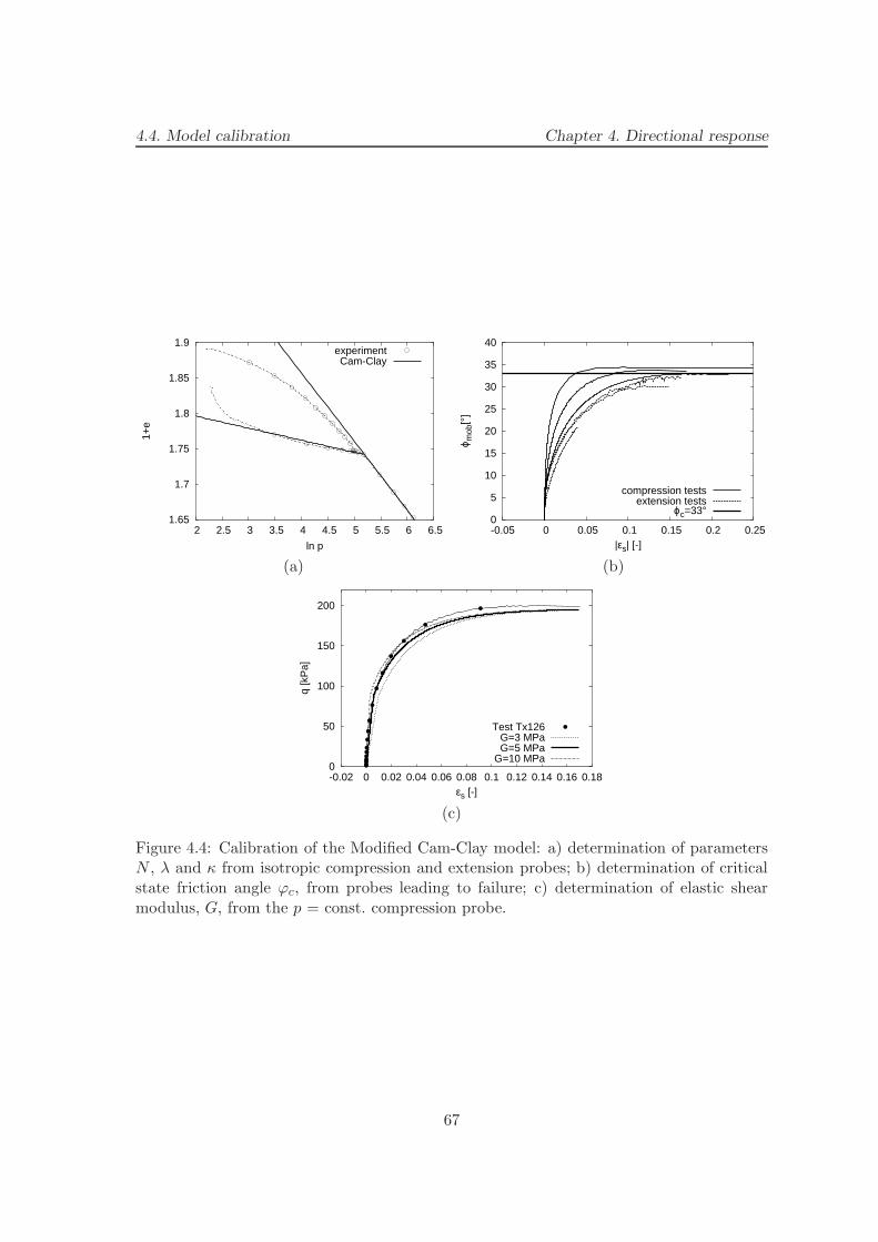
4.4. Model calibration Chapter 4. Directional response
1.65
1.7
1.75
1.8
1.85
1.9
2 2.5 3 3.5 4 4.5 5 5.5 6 6.5
1+e
ln p
experimentCam-Clay
(a)
0
5
10
15
20
25
30
35
40
-0.05 0 0.05 0.1 0.15 0.2 0.25
ϕ mob
[°]
|εs| [-]
compression testsextension tests
ϕc=33°
(b)
0
50
100
150
200
-0.02 0 0.02 0.04 0.06 0.08 0.1 0.12 0.14 0.16 0.18
q [k
Pa]
εs [-]
Test Tx126G=3 MPaG=5 MPa
G=10 MPa
(c)
Figure 4.4: Calibration of the Modified Cam-Clay model: a) determination of parametersN , λ and κ from isotropic compression and extension probes; b) determination of criticalstate friction angle ϕc, from probes leading to failure; c) determination of elastic shearmodulus, G, from the p = const. compression probe.
67

4.4. Model calibration Chapter 4. Directional response
for p = p0 with the N and λ values given in Tab. 4.3. Therefore, the initial value of thepreconsolidation pressure pc0 (i.e., the size of the elliptical yield locus along the isotropicaxis) is slightly larger than p0 and the soil appears as slightly overconsolidated (“quasi-preconsolidation” effect). The value of pc0 consistent with the assumed position of thevirgin compression line and initial void ratio can be computed by the following equation:
1 + e0 = N − λ ln pc0 + κ lnpc0p0
(4.11)
with p0 and e0 provided by Tab. 4.2 and N , λ and κ as in Tab. 4.3.
4.4.2 3–SKH model
In the 3–SKH model, the material constants λ∗ and N∗ define the slope and position ofthe virgin compression line in the ln(1 + e):ln p plane. Their numerical values have beendetermined by interpolating the experimental data from the isotropic compression probe,Tx128, shown in Fig. 4.4a.
According to eq. (4.34)2 of Appendix B, the constants A, m and n quantify the dependenceof the elastic shear modulus G on mean effective stress p and preconsolidation pressure2a (size of the Bounding Surface along the isotropic axis). Due to the lack of reliableinformation on the influence of such state variables on G, the values for the constants mand n have been set equal to those provided by Masın [86] for London Clay. The constantA was determined by comparing the shear stiffness value predicted by eq. (4.34)2 with thetangent shear moduli measured in a number of deviatoric probes (Tx121–Tx123, Tx125
and Tx126) at very small strain levels. These tangent shear moduli are plotted in Fig. 4.5aas a function of the deviatoric strain. From the figure, it is apparent how the experimentaldata in the very small strain range (ǫs < 1.0 · 10−4) are quite scattered, due to the lackof accurate strain measurements. For the purpose of model calibration, the average valueA = 653 was selected, which is well inside the range of values reported for similar soils.
The constant κ∗ controls the value of the bulk modulus of the material in the elastic range,see eq. (4.34)3. In principle, it could be determined from the isotropic extension probe,Tx127, as the slope of the tangent to the unloading curve in the ln(1+e):ln p plane at verysmall volumetric strains. However, due to the lack of accurate volume change measurementsin the very small strain range, κ∗ was determined from the elastic shear stiffness, as:
κ∗ =p
K=
3(1 − 2ν)
2(1 + ν)
p
G
by assuming a value of the Poissons ratio ν = 0.25, at p = 150 kPa.
The parameter M , controlling the slope of the Critical State Line for axisymmetric com-pression in the q:p plane can be assumed equal to 1.33, as for the Modified Cam-Claymodel. No ad-hoc experimental tests were performed to calibrate the parameters T and S.Therefore, in lack of sufficient information and since the values reported in the literaturefor these two constants lie in a very narrow range – see References [125, 7, 65, 86] – thevalues determined by Masın [86] for London Clay were adopted.
68

4.4. Model calibration Chapter 4. Directional response
0
5
10
15
20
25
30
35
1e-05 0.0001 0.001 0.01 0.1
G [M
Pa]
εs [-]
test Tx121test Tx126test Tx123test Tx125test Tx122
A=653
(a)
0
50
100
150
200
-0.02 0 0.02 0.04 0.06 0.08 0.1 0.12 0.14 0.16 0.18
q [k
Pa]
εs [-]
Test Tx126ψ=0.5
ψ=1ψ=1.5
(b)
Figure 4.5: Calibration of the 3–SKH model: a) determination of parameter A from devi-atoric probes; b) determination of parameter ψ from the p = const. compression probe.
The last material constant of the model – namely the exponent ψ appearing in the expres-sion of the hardening moduli H1 and H2, eq. (4.51) – was determined by trial and error,by comparing the model response with the experimental results obtained in the p = const.compression probe Tx126. From the results shown in Fig. 4.5b, a value of ψ = 1.0 hasbeen considered appropriate.
The complete set of parameters for the 3–SKH model is summarized in Tab. 4.4.
N∗ λ∗ A n m κ∗ M T S ψ
0.85 0.057 653 0.71 † 0.27 † 0.004 1.33 0.24 † 0.16 † 1.0
Table 4.4: Parameters of the 3–SKH model. Quantities indicated with the symbol † havebeen assumed from data reported by Masın [86] for London Clay.
The definition of the initial conditions requires the determination of the initial values ofthe internal variable a – controlling the size of the elliptic Bounding Surface, see eq. (4.38)– and of the two back-stresses, σa and σb, defining the centers of the yield surface andhistory surface, respectively (see Fig. 4.3).
As previously discussed in sect. 4.4.1, the initial state of the material appears to be slightlyoverconsolidated due to the quasi-preconsolidation effect induced by creep strains. Indefining the initial value of the parameter a, this effect can be easily taken into accountby fixing the position of the virgin compression line of the material. From the expressionsof the virgin compression and unloading/reloading curves in the ln(1 + e):ln p plane, thefollowing relation between a and the initial void ratio e0 and mean stress p0 can be derived:
ln (1 + e0) = N − λ∗ ln 2a+ κ∗ ln2a
p0(4.12)
Eq. (4.12) can be solved for a, with p0 and e0 provided by Tab. 4.2 and N∗, λ∗ and κ∗ as
69
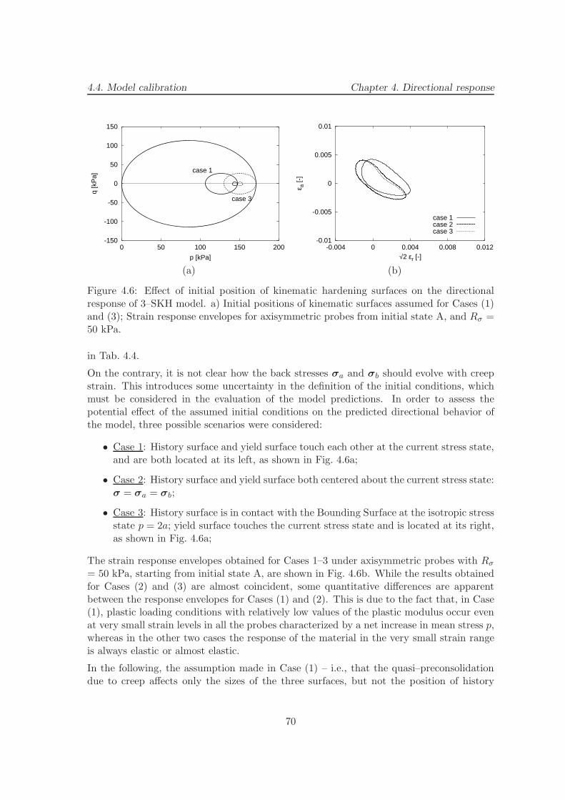
4.4. Model calibration Chapter 4. Directional response
-150
-100
-50
0
50
100
150
0 50 100 150 200
q [k
Pa]
p [kPa]
case 1
case 3
(a)
-0.01
-0.005
0
0.005
0.01
-0.004 0 0.004 0.008 0.012
ε a [-
]
√2 εr [-]
case 1case 2case 3
(b)
Figure 4.6: Effect of initial position of kinematic hardening surfaces on the directionalresponse of 3–SKH model. a) Initial positions of kinematic surfaces assumed for Cases (1)and (3); Strain response envelopes for axisymmetric probes from initial state A, and Rσ =50 kPa.
in Tab. 4.4.
On the contrary, it is not clear how the back stresses σa and σb should evolve with creepstrain. This introduces some uncertainty in the definition of the initial conditions, whichmust be considered in the evaluation of the model predictions. In order to assess thepotential effect of the assumed initial conditions on the predicted directional behavior ofthe model, three possible scenarios were considered:
• Case 1: History surface and yield surface touch each other at the current stress state,and are both located at its left, as shown in Fig. 4.6a;
• Case 2: History surface and yield surface both centered about the current stress state:σ = σa = σb;
• Case 3: History surface is in contact with the Bounding Surface at the isotropic stressstate p = 2a; yield surface touches the current stress state and is located at its right,as shown in Fig. 4.6a;
The strain response envelopes obtained for Cases 1–3 under axisymmetric probes with Rσ= 50 kPa, starting from initial state A, are shown in Fig. 4.6b. While the results obtainedfor Cases (2) and (3) are almost coincident, some quantitative differences are apparentbetween the response envelopes for Cases (1) and (2). This is due to the fact that, in Case(1), plastic loading conditions with relatively low values of the plastic modulus occur evenat very small strain levels in all the probes characterized by a net increase in mean stress p,whereas in the other two cases the response of the material in the very small strain rangeis always elastic or almost elastic.
In the following, the assumption made in Case (1) – i.e., that the quasi–preconsolidationdue to creep affects only the sizes of the three surfaces, but not the position of history
70

4.4. Model calibration Chapter 4. Directional response
-150
-100
-50
0
50
100
150
0 20 40 60 80 100 120 140 160 180 200
q [k
Pa]
p [kPa]
state A
(a)
-150
-100
-50
0
50
100
150
0 20 40 60 80 100 120 140 160 180 200
q [k
Pa]
p [kPa]
state B
(b)
Figure 4.7: Initial configuration assumed for the kinematic surfaces of 3–SKH model: a)initial state A; b) initial state B. Stress probe directions are also shown in the figures.
and yield surfaces with respect to the current stress state – has been assumed both for thecalibration of the 3–SKH model and for the simulation of the stress probing experimentsfrom state B, discussed in Sect. 4.5. The initial configuration assumed for the kinematicsurfaces for states A ad B is shown in Fig. 4.7. Note that, while the state A appears asslightly overconsolidated, according to the value of the average initial void ratio reportedin Tab. 4.2, the state B lies on the Bounding Surface. The initial configuration of thekinematic hardening surfaces at state B, shown in Fig. 4.7b, is the only possible underthe assumption of Case (1), due to the non-intersection condition. However, it is worthrecalling that Clayton and Heymann [30] report experimental evidence showing an initiallystiff, “elastic” behavior after some period of rest.
4.4.3 CLoE hypoplastic model
As discussed by Chambon et al. [29], the calibration of the CLoE model requires experi-mental data from some prescribed “basic paths”, including:
i) conventional drained triaxial compression and extension;
ii) isotropic compression or extension;
iii) “pseudo-isotropic” (i.e., isotropic loading from an anisotropic stress state) compres-sion and extension.
Four of these basic paths are included among the stress probes originating from the isotropicinitial state A (Tx121, Tx122 and Tx127 or Tx128). As for the pseudo-isotropic tests,use was made of the results of the stress probe Tx115, originating from the initial stateB. This is the only case in which some information from the stress-probing experimentsconducted from the anisotropic state B was used in the calibration process.
71

4.4. Model calibration Chapter 4. Directional response
The various constants of the CLoE model cannot be evaluated directly from the experi-mental results, since care must be taken in preserving the consistency of the constitutivetensors at isotropic states and on the limit surface, which bounds the region of admissiblestress states in stress space. Rather, a complex calibration procedure must be followedin order to obtain a consistent set of parameters, see Reference [29] for details. In thiscase, the calibration procedure was carried out using a specifically designed software tool,kindly provided by Desrues [42]. The results of the calibration process are summarizedin Tab. 4.5, providing the complete set of parameters adopted in the simulations with theCLoE model.
ϕc c χca yca yrc pfc pref ǫv,ref λc ϕe(deg) (kPa) (–) (–) (–) (–) (kPa) (–) (–) (deg)
34.0 0 0.17 0.055 3.1 0 147.26 0.0 183.34 33
χd χc χm2 ye pfe mc me† n † ω †
(–) (–) (–) (–) (–) (–) (–) (–) (–)
-1.0 -0.1 -0.05 0.011 0.02 -0.2 0.0 -0.2 0.36
Table 4.5: Parameters of the CLoE model. Quantities indicated with the symbol † havebeen estimated according to Desrues [42].
The comparison between model predictions and material response observed on the calibra-tion paths is shown in Fig. 4.8. The model provides a fairly good match with experimentalresults for all calibration paths, with the only exception of the isotropic compression path(Fig. 4.8c), for which the model significantly underestimates the compressibility of the soil.This clear limitation is due to the fact that, in its current version, the model does not allowto prescribe independently the bulk and shear tangent moduli (in both compression andextension) at isotropic states, see Reference [92]. A change in the bulk stiffness in isotropiccompression is reflected in the deviatoric response, so that any attempt to improve themodel response in isotropic compression would unavoidably deteriorate the performanceof the model along the other paths. The set of parameters shown in Tab. 4.5 was takenas the best possible compromise in terms of predictive capability of the model along theentire set of basic paths.
4.4.4 K-hypoplastic models for clays
A detailed discussion of the procedures required for the calibration of the K-hypoplasticmodel for clays can be found in Reference [87]. The standard version of the model is fullycharacterized by five constitutive constants, namely N∗, λ∗, κ∗, ϕc and r.
The constants N∗ and λ∗ control the position and slope of the isotropic normal compressionline in the ln(1 + e):ln p plane. As such, they have the same physical meaning as thecorresponding constants of the 3–SKH model (Sect. 4.3.1), and can be determined asdiscussed in Sect. 4.4.2. For the determination of the constant κ∗ – which controls the
72
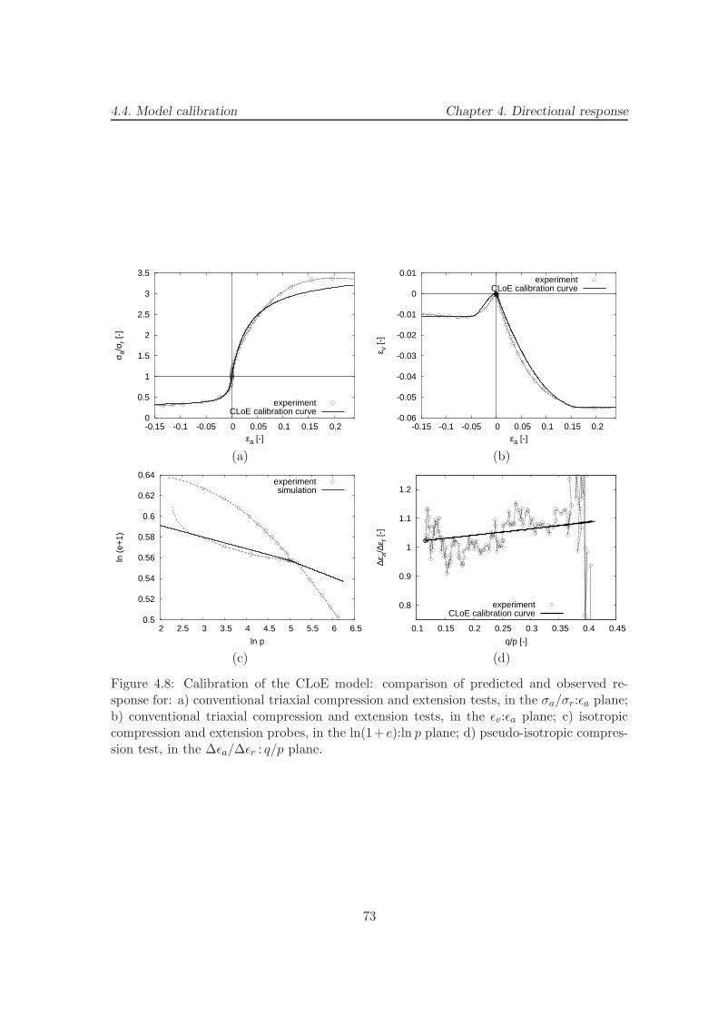
4.4. Model calibration Chapter 4. Directional response
0
0.5
1
1.5
2
2.5
3
3.5
-0.15 -0.1 -0.05 0 0.05 0.1 0.15 0.2
σ a/σ
r [-]
εa [-]
experiment CLoE calibration curve
(a)
-0.06
-0.05
-0.04
-0.03
-0.02
-0.01
0
0.01
-0.15 -0.1 -0.05 0 0.05 0.1 0.15 0.2
ε v [-
]
εa [-]
experiment CLoE calibration curve
(b)
0.5
0.52
0.54
0.56
0.58
0.6
0.62
0.64
2 2.5 3 3.5 4 4.5 5 5.5 6 6.5
ln (
e+1)
ln p
experimentsimulation
(c)
0.8
0.9
1
1.1
1.2
0.1 0.15 0.2 0.25 0.3 0.35 0.4 0.45
∆εa/
∆εr [
-]
q/p [-]
experimentCLoE calibration curve
(d)
Figure 4.8: Calibration of the CLoE model: comparison of predicted and observed re-sponse for: a) conventional triaxial compression and extension tests, in the σa/σr:ǫa plane;b) conventional triaxial compression and extension tests, in the ǫv:ǫa plane; c) isotropiccompression and extension probes, in the ln(1+ e):ln p plane; d) pseudo-isotropic compres-sion test, in the ∆ǫa/∆ǫr : q/p plane.
73

4.4. Model calibration Chapter 4. Directional response
0.5
0.52
0.54
0.56
0.58
0.6
0.62
0.64
0.66
2 2.5 3 3.5 4 4.5 5 5.5 6 6.5
ln (
e+1)
ln p
experimentclay K-hypoplas., basic
(a)
0
50
100
150
200
-0.02 0 0.02 0.04 0.06 0.08 0.1 0.12 0.14 0.16 0.18
q [k
Pa]
εs [-]
Test Tx126r=0.2r=0.4r=0.6
(b)
Figure 4.9: Calibration of the K-hypoplastic model for clays: comparison of predicted andobserved response for: a) isotropic compression and extension tests, in the ln(1 + e):ln pplane; b) constant p triaxial compression, in the q:ǫs plane.
compressibility of the soil in isotropic unloading – the choice has been made to use theresults of the stress probe Tx127 in the medium strain range. A reasonably good fit tothe available experimental data was obtained with κ∗ = 0.007, as shown in Fig. 4.9a.
The constant ϕc defines the friction angle of the material in critical state conditions. Itsdetermination has been already discussed in Sect. 4.4.1. The last constant, r, controls theratio between shear and bulk stiffness in isotropic virgin states. It was calibrated by trialand error, by comparing the model response with the experimental data from the stressprobe Tx126, i.e., a constant p compression test from the isotropic virgin state A. Thebest fit between predictions and measurements was obtained with r = 0.4, see Fig. 4.9b.
The extension of the K-hypoplastic model to include the effects of previous loading historyby means of the intergranular strain concept requires five additional constants to be iden-tified, namely mR, mT , R, βr and χ (see Reference [108]). In principle, their calibrationrequires experimental data from non-conventional laboratory experiments involving com-plex loading paths – such as those considered by Atkinson et al. [6] in the experimentalevaluation of the effects of recent stress history – and small-strain stiffness measurementsusing dynamic testing techniques. Such experiments are not included in the experimentalprogram considered in this study. However, as suggested by Masın [87], the constants R,βr and χ, which provide the extent of the quasi-elastic range for the material and thestiffness degradation rate with increasing strain, typically show a relatively limited rangeof variation for different soils, and therefore have been estimated with reference to theexperimental data available for London Clay [86].
The constant mR, which controls the hypo-elastic stiffness upon stress path reversal in thevery small strain range, was estimated by means of the following relation between mR and
74
4.5. Comparison of predictions Chapter 4. Directional response
the small-strain shear modulus G0 in isotropic conditions [87]:
G0 ≃ mRp
rλ∗⇔ mR ≃ G0rλ
∗
p(4.13)
with G0 = 23.0 MPa at p = 150 kPa, see Fig. 4.5a. This guarantees that the enhancedK-hypoplastic model and the 3–SKH model are characterized by identical shear stiffnessesin the very small strain range. Finally, in the absence of any other experimental indication,mT was assumed equal to mR. The results of the calibration process are summarized inTab. 4.6.
N∗ λ∗ κ∗ ϕc r mR mT R βr χ(–) (–) (–) (deg) (–) (–) (–) (–) (–) (–)
0.85 0.057 0.007 33.0 0.4 3.5 3.5 10−4 † 0.2 † 6.0 †
Table 4.6: Parameters of the K-hypoplastic models for clays. Quantities indicated withthe symbol † were assumed from data reported by Masın [86] for London Clay.
The definition of the initial conditions requires the determination of the initial values ofthe void ratio and of the intergranular strain tensor δ. As for the void ratio, the valuesprovided in Tab. 4.2 were adopted. Note that, with the values of N∗ and λ∗ given inTab. 4.6, the void ratio assumed for the isotropic state A is slightly lower than the voidratio on the virgin compression line at the same mean stress. This implies that the materialappears slightly overconsolidated, as already noted in Sect. 4.4.2. The initial values of theintergranular strain for the two states A and B were determined by numerically simulatingthe two constant q/p compression paths imposed to the material before the start of thestress-probing. This guarantees that the initial values of δ are consistent with the initialconfiguration of the kinematic surfaces in the 3–SKH model.
4.5 Comparison of observed and predicted response
4.5.1 Strain response envelopes
In the following, the response of reconstituted Beaucaire Marl to the stress probing programdetailed in Tab. 4.1, as well as the predictions of the different models described above, isdepicted by using the so-called incremental strain response envelope, as defined in Reference[133]. Such a representation directly follows from the concept of stress response envelope,first proposed by Gudehus [50] as a convenient tool for visualizing the properties of rate-typeconstitutive equations. According to Gudehus, a stress (strain) response envelope is definedas the image in the stress (strain) rate space of the unit sphere in the strain (stress) ratespace, under the map defined by the constitutive equation. By simply replacing rates withfinite-size increments, the same definitions apply to the incremental response envelopes.In the general case, an incremental strain response envelope (RE, hereafter) is a surface
75

4.5. Comparison of predictions Chapter 4. Directional response
in a six-dimensional space. However, for the particular loading conditions considered, themost natural choice is to represent the section of the REs in the plane of work-conjugatedstrain increment quantities, (∆ǫa,
√2 ∆ǫr), see Fig. 4.1b. The size of each strain increment
vector defining the RE can be directly interpreted as a directional secant compliance of thematerial, for the associated loading direction and stress increment magnitude.
Figures 4.10 and 4.11 show the computed REs for all the models considered at small tomedium stress increment levels (Rσ = 20, 30, 40 and 50 kPa), and at medium to large stressincrement levels (Rσ = 50 and 90 kPa), respectively. The corresponding experimentallyobtained REs are also shown in both figures on the top left corner.
For small to medium stress increment levels, the experimental REs indicate that the softestresponse is associated with those paths which are characterized by a large deviatoric com-ponent (e.g., tests Tx119 and Tx113). As Rσ increases, the envelopes progressively shiftupward to the left, due to the fact that the initial state is closer to the critical state linefor axisymmetric compression than to the corresponding line for axisymmetric extension.For η = 0.4 loading paths (Tx130 and Tx129), the material response is softer when theprobe points in the direction of continued loading, and stiffer upon unloading (i.e., uponfull stress path reversal with respect to the consolidation history). In fact, this last pathcorresponds to the stiffest response of the material. A direct consequence of the aboveobservations is that the experimental REs are markedly non-symmetric about the originof the strain increment space.
The predictions of the different models considered appear, from a qualitative standpoint,all in fair agreement with the salient features of the experimental response discussed above.The only notable exception is represented by the predictions of CLoE model upon η = 0.4loading paths, where – contrary to experimental evidence – no significant difference betweensecant stiffness in compression and extension is observed. From a quantitative standpoint,however, all models appear to significantly underpredict the secant stiffness of the material.The REs predicted with the two elastoplastic models show a convex shape, except for theexpected, yet minor irregularity of the Modified Cam-Clay envelopes, close to neutralloading in extension. The REs of the two K-hypoplastic models, and (to a much lesserextent) those of CLoE show some degree of non-convexity in a region located around theη = 0.4 loading direction. This feature is also shown by the two largest experimental REs,although such an observation is based on the results of one single stress-probe.
At large stress increment level (Rσ = 90 kPa, Fig. 4.11), both the elastoplastic and theK-hypoplastic models provide response envelopes which appear in fairly good agreementwith the experimental results, from both a qualitative and a quantitative point of view.On the contrary, CLoE significantly overestimates soil stiffness for loading paths close todeviatoric compression (Tx116 and Tx119).
4.5.2 Normalized stress-paths
In addition to response envelopes, the performance of the five models can be also assessedby representing the prescribed stress paths in the normalized plane q/p∗e : p/p∗e, where p∗e
76
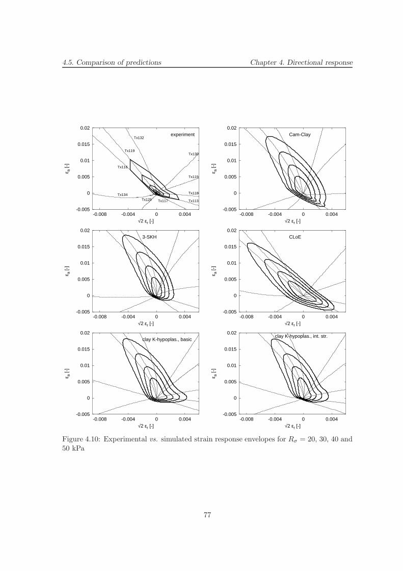
4.5. Comparison of predictions Chapter 4. Directional response
-0.005
0
0.005
0.01
0.015
0.02
-0.008 -0.004 0 0.004
ε a [-
]
√2 εr [-]
experimentTx132
Tx119
Tx116
Tx134Tx129 Tx117 Tx113
Tx118
Tx115
Tx130
-0.005
0
0.005
0.01
0.015
0.02
-0.008 -0.004 0 0.004ε a
[-]
√2 εr [-]
Cam-Clay
-0.005
0
0.005
0.01
0.015
0.02
-0.008 -0.004 0 0.004
ε a [-
]
√2 εr [-]
3-SKH
-0.005
0
0.005
0.01
0.015
0.02
-0.008 -0.004 0 0.004
ε a [-
]
√2 εr [-]
CLoE
-0.005
0
0.005
0.01
0.015
0.02
-0.008 -0.004 0 0.004
ε a [-
]
√2 εr [-]
clay K-hypoplas., basic
-0.005
0
0.005
0.01
0.015
0.02
-0.008 -0.004 0 0.004
ε a [-
]
√2 εr [-]
clay K-hypoplas., int. str.
Figure 4.10: Experimental vs. simulated strain response envelopes for Rσ = 20, 30, 40 and50 kPa
77
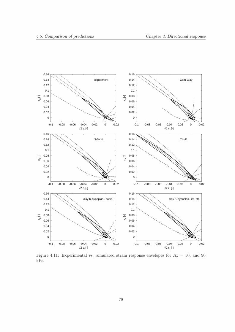
4.5. Comparison of predictions Chapter 4. Directional response
0
0.02
0.04
0.06
0.08
0.1
0.12
0.14
0.16
-0.1 -0.08 -0.06 -0.04 -0.02 0 0.02
ε a [-
]
√2 εr [-]
experiment
0
0.02
0.04
0.06
0.08
0.1
0.12
0.14
0.16
-0.1 -0.08 -0.06 -0.04 -0.02 0 0.02ε a
[-]
√2 εr [-]
Cam-Clay
0
0.02
0.04
0.06
0.08
0.1
0.12
0.14
0.16
-0.1 -0.08 -0.06 -0.04 -0.02 0 0.02
ε a [-
]
√2 εr [-]
3-SKH
0
0.02
0.04
0.06
0.08
0.1
0.12
0.14
0.16
-0.1 -0.08 -0.06 -0.04 -0.02 0 0.02
ε a [-
]
√2 εr [-]
CLoE
0
0.02
0.04
0.06
0.08
0.1
0.12
0.14
0.16
-0.1 -0.08 -0.06 -0.04 -0.02 0 0.02
ε a [-
]
√2 εr [-]
clay K-hypoplas., basic
0
0.02
0.04
0.06
0.08
0.1
0.12
0.14
0.16
-0.1 -0.08 -0.06 -0.04 -0.02 0 0.02
ε a [-
]
√2 εr [-]
clay K-hypoplas., int. str.
Figure 4.11: Experimental vs. simulated strain response envelopes for Rσ = 50, and 90kPa
78
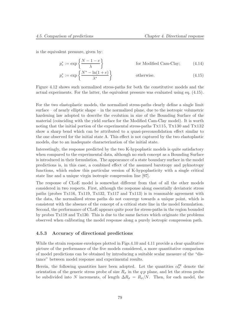
4.5. Comparison of predictions Chapter 4. Directional response
is the equivalent pressure, given by:
p∗e := exp
{
N − 1 − e
λ
}
for Modified Cam-Clay; (4.14)
p∗e := exp
{
N∗ − ln(1 + e)
λ∗
}
otherwise. (4.15)
Figure 4.12 shows such normalized stress-paths for both the constitutive models and theactual experiments. For the latter, the equivalent pressure was evaluated using eq. (4.15).
For the two elastoplastic models, the normalized stress-paths clearly define a single limitsurface – of nearly elliptic shape – in the normalized plane, due to the isotropic volumetrichardening law adopted to describe the evolution in size of the Bounding Surface of thematerial (coinciding with the yield surface for the Modified Cam-Clay model). It is worthnoting that the initial portion of the experimental stress-paths Tx115, Tx130 and Tx132
show a sharp bend which can be attributed to a quasi-preconsolidation effect similar tothe one observed for the initial state A. This effect is not captured by the two elastoplasticmodels, due to an inadequate characterization of the initial state.
Interestingly, the response predicted by the two K-hypoplastic models is quite satisfactorywhen compared to the experimental data, although no such concept as a Bounding Surfaceis introduced in their formulation. The appearance of a state boundary surface in the modelpredictions is, in this case, a combined effect of the assumed barotropy and pyknotropyfunctions, which endow this particular version of K-hypoplasticity with a single criticalstate line and a unique virgin isotropic compression line [97].
The response of CLoE model is somewhat different from that of all the other modelsconsidered in two respects. First, although the response along essentially deviatoric stresspaths (probes Tx116, Tx119, Tx132, Tx117 and Tx113) is in reasonable agreement withthe data, the normalized stress paths do not converge towards a unique point, which isconsistent with the absence of the concept of a critical state line in the model formulation.Second, the performance of CLoE appears quite poor for stress-paths in the region boundedby probes Tx118 and Tx130. This is due to the same factors which originate the problemsobserved when calibrating the model response along a purely isotropic compression path.
4.5.3 Accuracy of directional predictions
While the strain response envelopes plotted in Figs.4.10 and 4.11 provide a clear qualitativepicture of the performance of the five models considered, a more quantitative comparisonof model predictions can be obtained by introducing a suitable scalar measure of the “dis-tance” between model response and experimental results.
Herein, the following quantities have been adopted. Let the quantities αpqσ denote theorientation of the generic stress probe of size Rσ in the q:p plane, and let the stress probebe subdivided into N increments, of length ∆Rσ = Rσ/N . Then, for each model, the
79
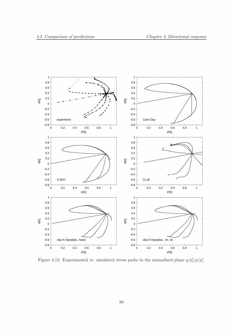
4.5. Comparison of predictions Chapter 4. Directional response
-0.8
-0.6
-0.4
-0.2
0
0.2
0.4
0.6
0.8
1
0 0.2 0.4 0.6 0.8 1
q/p* e
p/p*e
experiment
-0.8
-0.6
-0.4
-0.2
0
0.2
0.4
0.6
0.8
1
0 0.2 0.4 0.6 0.8 1q/
p* e
p/p*e
Cam-Clay
-0.8
-0.6
-0.4
-0.2
0
0.2
0.4
0.6
0.8
1
0 0.2 0.4 0.6 0.8 1
q/p* e
p/p*e
3-SKH
-0.8
-0.6
-0.4
-0.2
0
0.2
0.4
0.6
0.8
1
0 0.2 0.4 0.6 0.8 1
q/p* e
p/p*e
CLoE
-0.8
-0.6
-0.4
-0.2
0
0.2
0.4
0.6
0.8
1
0 0.2 0.4 0.6 0.8 1
q/p* e
p/p*e
clay K-hypoplas., basic
-0.8
-0.6
-0.4
-0.2
0
0.2
0.4
0.6
0.8
1
0 0.2 0.4 0.6 0.8 1
q/p* e
p/p*e
clay K-hypoplas., int. str.
Figure 4.12: Experimental vs. simulated stress paths in the normalized plane q/p∗e:p/p∗e.
80

4.5. Comparison of predictions Chapter 4. Directional response
simulation error err(αpqσ , Rσ) can be defined as:
err(αpqσ , Rσ) =N∑
k=1
∥
∥
∥∆ǫ
(k)sim − ∆ǫ(k)
exp
∥
∥
∥(4.16)
where ∆ǫ(k)exp and ∆ǫ
(k)sim are the measured and predicted strain increment tensors, respec-
tively, corresponding to the k-th stress increment of size ∆Rσ.
To assess the relative size of the prediction error, as compared to the strain-path length, asecond, normalized error measure is introduced as follows:
errnorm(αpqσ , Rσ) =err(αpqσ , Rσ)∑N
k=1
∥
∥
∥∆ǫ
(k)exp
∥
∥
∥
(4.17)
Figures 4.13 and 4.14 show computed values of err and errnorm as a function of the probedirection αpqσ . Two stress increment ranges have been considered, namely Rσ = 30 kPa(Fig. 4.13) and Rσ = 90 kPa (Fig. 4.14). In both cases, the evaluation of the two errormeasures has been carried out with ∆Rσ = 5 kPa, which was considered to be the smalleststress increment for which experimental results are not significantly affected by scatter inthe measurements.
For Rσ = 30 kPa, the performance of the two elastoplastic models is compared in Fig. 4.13a.The largest prediction error, err ≃ 0.006, corresponds to probe directions with αpqσ around72◦ (conventional triaxial compression). This is a consequence of the fact that, whilethe initial state for the two models lies on the Bounding Surface, the experimental dataclearly indicate that the soil possesses some degree of overconsolidation (see Fig. 4.12),probably induced by creep strains accumulated during the rest period before probing.The best predictions, in absolute terms, are obtained in the range 200◦ < αpqσ < 300◦.This is not surprising, since in this region the response of the two models is quite stiff,hence the strain increment magnitudes are quite small. The effect of loading directionis less important when considering the relative error, errnorm, as this quantity accountsfor the dependence of soil stiffness on loading direction. The two models provide almostidentical predictions for the entire range of probing directions, except for the zone in whichModified Cam-Clay undergoes elastic unloading (200◦ < αpqσ < 300◦). Again, this is tobe expected, since when the initial state is on the Bounding Surface, the 3–SKH modelbehaves as a standard Modified Cam-Clay for all probes which are directed outwards. Onthe contrary, when the stress-probes are directed inwards, then the more evoluted nestedsurface kinematic hardening structure of the 3–SKH model is capable of reproducing muchbetter the experimental response, in both absolute and relative terms.
For the same stress increment range, the performance of the hypoplastic models is shownin Fig. 4.13b. The computed absolute error distributions with probe direction are quitesimilar, both in shape and magnitude, to those of the two elastoplastic models. Thesame is also true, to a certain extent, for the normalized error. The response of the twoK-hypoplastic models is almost coincident for those probes corresponding to continued
81

4.5. Comparison of predictions Chapter 4. Directional response
0
1
2
3
4
5
6
0 45 90 135 180 225 270 315 360
0
0.002
0.004
0.006
0.008
0.01
err n
orm
[-]
err
[-]
ασpq [°]
3-SKHCam-Clay
(a)
0
1
2
3
4
5
6
0 45 90 135 180 225 270 315 360
0
0.002
0.004
0.006
0.008
0.01
err n
orm
[-]
err
[-]
ασpq [°]
clay K-hypoplas., int. str.clay K-hypoplas., basic
CLoE
(b)
Figure 4.13: Scalar error measures with respect to the stress-path direction αpqσ in the p:qplane at state B, Rσ = 0 − 30 kPa
0
1
2
3
4
5
6
0 45 90 135 180 225 270 315 360
0
0.01
0.02
0.03
0.04
err n
orm
[-]
err
[-]
ασpq [°]
3-SKHCam-Clay
(a)
0
1
2
3
4
5
6
0 45 90 135 180 225 270 315 360
0
0.01
0.02
0.03
0.04
err n
orm
[-]
err
[-]
ασpq [°]
clay K-hypoplas., int. str.clay K-hypoplas., basic
CLoE
(b)
Figure 4.14: Scalar error measures with respect to the stress-path direction αpqσ in the p:qplane at state B, Rσ = 0 − 90 kPa
82

4.6. Concluding remarks Chapter 4. Directional response
loading conditions, as in this case the material reaches quite rapidly the swept-out-memoryconditions. Under reverse loading conditions, the two responses diverge and, as expected,the K-hypoplastic model with intergranular strains performs significantly better. This iseven more apparent when considering the normalized error plots. For the same range ofprobe directions, CLoE performance appears to be substantially poorer, both in absoluteand relative terms. On the contrary, for continued loading conditions (340◦ < αpqσ <90◦) CLoE provides the best results among all the models considered. In fact, this is aconsequence of a fortuitous combination of two different factors. On the one hand, CLoEcalibration has clearly shown that the model is not capable of correctly reproducing thelarge decrease in stiffness associated with virgin loading upon isotropic or η = const. loadingconditions. On the other hand, the actual response of the material for the same range ofprobing directions appears to be much stiffer than expected for a material in a virgin state,due to the quasi-preconsolidation effect already mentioned.
Overall, data reported in Fig. 4.13 indicate that the best performance is provided by the 3–SKH model and the K-hypoplastic model with intergranular strains, which appear to yieldquite similar results in terms of prediction error measures. A somehow different pictureemerges by looking at the results for the larger stress increment range (Fig. 4.14). In thiscase, not only the relative error levels are generally lower, but also the differences betweenthe models are less important. In fact, Modified Cam-Clay performs almost as well as themore refined 3–SKH model, and the same applies to all the hypoplastic models, except forloading directions close to αpqσ = 180◦. In this case, roughly corresponding to a reductionof mean stress at q = const., CLoE performance is quite poor, while K-hypoplasticity withintergranular strain provides the best prediction among the models of this class, althoughnot as good as those of the two elastoplastic models.
4.6 Concluding remarks
The comparative evaluation of the performance of different constitutive models in theirapplication to the quantitative solution of practical engineering problems is a very complextask, which – in general – requires a careful consideration of several key factors, amongwhich we recall:
1. Qualitative and quantitative agreement between experimentally observed responseand model predictions at the element level (i.e., in the simulation of laboratorytests), in view of the main objectives of the analysis and the type of problem to besolved;
2. Relative complexity of the procedures required to determine the material constantsappearing in the model formulation;
3. Type and nature of the internal state variables entering the model to describe theeffects of previous loading history, and the relative complexity in the characterizationof their initial values;
83

4.6. Concluding remarks Chapter 4. Directional response
4. Availability of robust and accurate algorithms for the numerical implementation inFE codes, in view of the solution of the engineering problems at hand.
The comparison between model predictions and experimental results is typically done, inpractice, with reference to a limited number of more or less conventional stress paths,whereas the response of the material for different loading conditions is extrapolated in amore or less reasonable way. This can be quite sufficient to assess the model performancein those problems where most of the soil affected by the imposed loading conditions under-goes very similar stress paths, and one of such paths is included in the laboratory testingprogram. Unfortunately, this is only seldom the case in many important applications wherean accurate prediction of soil-structure interaction processes and of the displacement fieldaround the structure is required. Notable examples in this respect are provided by deepexcavations and shallow tunnels to be realized in urban environments, as in such cases,different zones of soil experience widely different stress-paths, both in size and direction,and the quality of numerical predictions crucially relies on the ability of the constitutivemodel adopted for the soil to accurately reproduce the material response along all suchloading paths.
In this paper, an attempt has been made to evaluate the response of different advancedconstitutive models for fine-grained soils in more general terms, considering their predic-tive capabilities over a quite wide range of loading conditions. In trying to compare theperformances of the different models, the experimental data of Costanzo et al. [31] havebeen considered as portraying the actual mechanical response of the soil. However, twomain points should be stressed in this respect. First, due to the time required to performeach test, only a few probes were duplicated, and thus most of the data on which theexperimental REs are constructed refer to a single specimen only. Therefore, the observedshape of the experimental REs might be affected to some extent by the unavoidable scatteralways present in experimental measurements. Second, the occurrence of small amounts ofviscous strains may affect both size and shape of the measured response envelopes, evenif to a limited extent, see Reference [31]. Interpreting the observed response in light ofrate-independent constitutive theories might therefore lead to an underestimation of soilstiffness for some probe directions and to an overestimation of soil stiffness for other probedirections, as thoroughly discussed in the companion paper [31].
Based on the normalized stress paths reported in Sect. 4.5.2 and the scalar error measuresintroduced in Sect. 4.5.3, the best performance overall appears to be provided by theintergranular strain-enhanced K-hypoplastic model for clays and the 3–SKH model, atboth small and large strain levels.
It is interesting to note that, since the soil considered in this study was in a (almost)normally consolidated state, the predictions of the classical Cam-Clay model for continuedloading conditions (i.e., those paths pointing outside the yield surface) are equivalent tothose obtained with the much more sophisticated 3–SKH model. In unloading, however,the data clearly show the substantial improvement of predictions which can be achievedwith the kinematic hardening approach.
84
4.6. Concluding remarks Chapter 4. Directional response
As compared to its enhanced version, the performance of the standard K-hypoplastic modelis still reasonably good, mainly because the loading programmes considered involve onlya very limited number of stress reversals. For the application to monotonic (or quasi-monotonic) loading conditions, the standard K-hypoplastic model may represents a validalternative to more complex formulations.
On the contrary, the performance of the CLoE model is definitely poor, when comparedwith the other elastoplastic or hypoplastic models, particularly for those loading pathsinvolving a significant increase in mean stress. This is not surprising, considering that CLoEis a first-generation hypoplastic model, in which the stress tensor is assumed as the onlystate variable for the material. For this reason, the mathematical structure of CLoE modeldoes not allow to properly distinguish normally consolidated and overconsolidated states,and to correctly describe critical state failure conditions. While CLoE has demonstratedits capability of accurately modelling the response of coarse-grained soils along mainlydeviatoric loading paths (see, e.g., Reference [29]), these limitations obviously make itunfit to model the behavior of natural clay deposits. An attempt to modify the currentversion of CLoE in order to improve its performance for normally consolidated clays hasbeen recently presented by Masın et al. [92].
Although the enhanced K-hypoplastic model and the 3–SKH model provide a great flex-ibility in describing the effects of recent stress history on the mechanical response of thesoil, they are both characterized by a relatively limited number of constants, most of whichare linked to standard features of clay behavior. All the constants appearing in these twomodels can be determined by means of standard laboratory tests, with the only exceptionof those controlling the stiffness of the material at very low strain levels. As discussed byMasın [87], these latter quantities can be easily determined from the results of dynamictests, such as bender element or resonant column tests.
On the contrary, the CLoE model requires a much wider pool of experimental data to cali-brate the large number of constants (19) appearing in the functions adopted to describe thematerial response along the selected basic paths. Moreover, as those parameters typicallycontrol more than one specific feature of the material response, they cannot be determinedindependently. Rather, they have to be found by means of a complex calibration procedurewhich has to be implemented numerically in a suitable calibration code. This represents asecond, major drawback of the CLoE model as compared to the more recent K-hypoplasticmodels for clays.
The characterization of the initial state of the material is relatively easy for Modified Cam-Clay, CLoE and standard K-hypoplastic models, for which only the initial values of thestress tensor and (possibly) one additional scalar state variable (preconsolidation pressureor void ratio) are required. Defining the initial state is more complex for the enhancedK-hypoplastic model and the 3–SKH model, since it requires the determination of one ortwo tensorial internal variables (the back-stresses or the intergranular strain). Even inthe simple case considered in this study, this has not been a trivial task. The difficultiesexperienced in the definition of the initial state have had an impact both on the results ofthe calibration procedures and on the prediction of the material response. It is reasonable
85

4.6. Concluding remarks Chapter 4. Directional response
to expect that such difficulties would increase in the application of those models to naturalclay deposits, with a more complicated – and possibly unknown – previous loading history.In such a case – based on some experimental observations of Jardine et al. [67] and Claytonand Heymann [30], who report an increase in soil stiffness for all loading directions after arelatively short resting period – Niemunis and Herle [108] suggest to assume δ = 0. Thisis equivalent to setting σa = σb = σ for the 3–SKH model.
Finally, as far as computational issues are concerned, it can be noted that robust andaccurate implicit or explicit integration algorithms are now available for both complexplasticity models (see, e.g., [16, 119, 84]) and advanced hypoplastic models (see, e.g.,[44, 40]). However, as the mathematical structure of the K-hypoplastic models appearssimpler than that of the 3–SKH model, or of any other kinematic hardening multisurfaceplasticity model, the former may have some advantage with respect to the latter as far astheir numerical implementation into existing FE codes is concerned.
Appendix A
The results of all the stress-probing tests from the anisotropic initial state B, along withthe corresponding predictions for the five models considered, are summarized in Figs. 4.15(q : ǫs plane) and 4.16 (p : ǫv plane). Note that all strain measures are evaluated as naturalstrains.
Appendix B: Mathematical formulation of the constitutivemodels
In the description of the relevant constitutive equations, the following invariant quantitiesfor the stress tensor are used:
p :=1
3σ : 1 q :=
√
3
2s : s cos(3θ) := −
√6
tr(
s3)
(s : s)3/2(4.18)
where s = σ − p1 is the deviatoric part of the stress tensor and 1 is the second-orderidentity tensor. Use is made of the fourth-order identity tensor I , with components:
(I)ijkl :=1
2(δikδjl + δilδjk) (4.19)
K-hypoplastic model for clays
The mathematical structure of the K-hypoplastic model for clays is discussed in detail inReference [87]. The constitutive equation in rate form reads:
σ = fsL : ǫ + fsfdN ‖ǫ‖ (4.20)
86

4.6. Concluding remarks Chapter 4. Directional response
-200
-100
0
100
200
300
-0.2 -0.15 -0.1 -0.05 0 0.05 0.1 0.15 0.2 0.25
q [k
Pa]
εs [-]
experiment
-200
-100
0
100
200
300
-0.2 -0.15 -0.1 -0.05 0 0.05 0.1 0.15 0.2 0.25
q [k
Pa]
εs [-]
Cam-Clay
-200
-100
0
100
200
300
-0.2 -0.15 -0.1 -0.05 0 0.05 0.1 0.15 0.2 0.25
q [k
Pa]
εs [-]
3-SKH
-200
-100
0
100
200
300
-0.2 -0.15 -0.1 -0.05 0 0.05 0.1 0.15 0.2 0.25
q [k
Pa]
εs [-]
CLoE
-200
-100
0
100
200
300
-0.2 -0.15 -0.1 -0.05 0 0.05 0.1 0.15 0.2 0.25
q [k
Pa]
εs [-]
clay K-hypoplas., basic
-200
-100
0
100
200
300
-0.2 -0.15 -0.1 -0.05 0 0.05 0.1 0.15 0.2 0.25
q [k
Pa]
εs [-]
clay K-hypoplas., int. str.
Figure 4.15: Experimental and predicted responses in the q:ǫs plane.
where:
L := 3(
c1I + c2a2σ ⊗ σ
)
N = L :
(
Ym
‖m‖
)
σ :=1
3pσ (4.21)
87

4.6. Concluding remarks Chapter 4. Directional response
0
50
100
150
200
250
300
350
400
450
500
-0.04 -0.02 0 0.02 0.04 0.06
p [k
Pa]
εv [-]
experiment
0
50
100
150
200
250
300
350
400
450
500
-0.04 -0.02 0 0.02 0.04 0.06p
[kP
a]
εv [-]
Cam-Clay
0
50
100
150
200
250
300
350
400
450
500
-0.04 -0.02 0 0.02 0.04 0.06
p [k
Pa]
εv [-]
3-SKH
0
50
100
150
200
250
300
350
400
450
500
-0.04 -0.02 0 0.02 0.04 0.06
p [k
Pa]
εv [-]
CLoE
0
50
100
150
200
250
300
350
400
450
500
-0.04 -0.02 0 0.02 0.04 0.06
p [k
Pa]
εv [-]
clay K-hypoplas., basic
0
50
100
150
200
250
300
350
400
450
500
-0.04 -0.02 0 0.02 0.04 0.06
p [k
Pa]
εv [-]
clay K-hypoplas., int. str.
Figure 4.16: Experimental and predicted responses in the p:ǫv plane.
88
4.6. Concluding remarks Chapter 4. Directional response
In eq. (4.20), the functions fs(p, e) (barotropy factor) and fd(e) (pyknotropy factor) aregiven by:
fs =3p
λ∗
(
3 + a2 − 2αa√
3)−1
fd =
{
2p exp
[
ln (1 + e) −N
λ∗
]}α
(4.22)
The scalar function Y and second-order tensor m appearing in eq. (4.21) are given, respec-tively, by:
Y =
( √3a
3 + a2− 1
)
(I1I2 + 9I3)(
1 − sin2 ϕc)
8I3 sin2 ϕc+
√3a
3 + a2(4.23)
in which:
I1 := tr(σ) I2 :=1
2
[
σ : σ − (I1)2]
I3 = detσ
and:
m = − a
F
[
σ + dev σ − σ
3
(
6σ : σ − 1
(F/a)2 + σ : σ
)]
(4.24)
in which:
F =
√
1
8tan2 ψ +
2 − tan2 ψ
2 +√
2 tanψ cos 3θ− 1
2√
2tanψ tanψ :=
√3 ‖dev σ‖ (4.25)
Finally, the scalars a, α, c1 and c2 appearing in eqs. (4.21)–(4.24), are given as functionsof the material parameters ϕc, λ
∗, κ∗ and r by the following relations:
a =
√3 (3 − sinϕc)
2√
2 sinϕcα =
1
ln 2ln
[
λ∗ − κ∗
λ∗ + κ∗
(
3 + a2
a√
3
)]
(4.26)
c1 =2(
3 + a2 − 2αa√
3)
9rc2 = 1 + (1 − c1)
3
a2(4.27)
The model requires five constitutive parameters, namely ϕc, λ∗, κ∗, N and r.
Integranular strain enhancement of K-hypoplasticity
As proposed by Niemunis and Herle [108], the enhanced K-hypoplastic model is endowedwith an additional state variable, δ, a second-order tensor defined as intergranular strain,which can be interpreted as a macroscopic manifestation of intergranular slips at graincontacts.
Let ρ := ‖δ‖ /R be a suitable normalized magnitude of δ, R being a scalar model parameter.Also, let
δ =
{
δ/‖δ‖ for δ 6= 00 for δ = 0
(4.28)
denote intergranular strain direction. The constitutive equations for enhanced K-hypoplasticityfor clays can be written as:
σ = M : ǫ (4.29)
89

4.6. Concluding remarks Chapter 4. Directional response
where the fourth-order tangent stiffness tensor M is calculated from the constitutive ten-sors tensors L and N defined in eq. (4.21), the barotropy and pyknotropy factors given ineq. (4.22), and the intergranular strain tensor via the following interpolation:
M = [ρχmT + (1 − ρχ)mR] fsL + B (4.30)
where:
B :=
{
ρχ (1 −mT ) fsL : δ ⊗ δ + ρχfsfdN ⊗ δ (δ : ǫ > 0)
ρχ (mR −mT ) fsL : δ ⊗ δ (δ : ǫ ≤ 0)(4.31)
and χ, mT and mR are material constants.
The evolution equation for the intergranular strain tensor δ is given by
δ =
{(
I − δ ⊗ δρβr
)
: ǫ (δ : ǫ > 0)
ǫ (δ : ǫ ≤ 0)(4.32)
As compared to the basic K-hypoplastic model for clay, the enhanced model requires fiveadditional parameters, namely R, mR, mT , βr and χ.
3-SKH model
The 3–SKH model is a nested-surface kinematic hardening plasticity model developed as anextension of classical Modified Cam-Clay. The original formulation is detailed in Reference[125]. Herein, the version proposed by Stallebrass and Taylor [127] is considered. Theevolution equation for the effective stress tensor is given by:
σ = De : (ǫ − ǫp) (4.33)
where ǫ is the plastic strain rate tensor and De is the elastic tangent stiffness tensor,defined by:
De :=
(
K − 2
3G
)
1 ⊗ 1 + 2GIG
pr= A
(
p
pr
)n( p
2a
)mK =
p
κ∗, (4.34)
In the above equations, the scalar quantity a is an internal variable to be defined later, pris a reference stress (set equal to 1.0 kPa), and A, n and m are model parameters.
Nonlinearity and irreversibility are introduced by requiring the stress state to belong tothe convex set (known as elastic domain):
Eσ :={
(σ, a,σb)∣
∣
∣f (σ, a,σb) ≤ 0
}
(4.35)
where f(σ, a,σb) is the yield function of the material, given by:
f(σ, a,σb) =1
2
[
( qbM
)2
+ p2b − T 2S2a2
]
(4.36)
90

4.6. Concluding remarks Chapter 4. Directional response
In eq. (4.36), the scalar functions pb and qb are the first and second invariants of the tensor(σ−σb), defined as in eq. (4.18); σb and a are internal variables, providing the coordinatesof the centers of the yield surface and of the Bounding Surface (see eq. (4.38)), respectively,and M, T and S are model parameters.
Inside the yield surface, ǫp = 0. For stress states on the yield surface, the plastic strainrate is given by the following associative flow rule:
ǫp =〈P : De : ǫ〉
H + P : De : PP P :=
∂f
∂σ(4.37)
where H is the plastic modulus and the operator 〈x〉 := (x + |x|)/2 denotes the positivepart of any scalar function x.
A key characteristic of the 3–SKH model is the definition of two additional surfaces instress space. The first one, known as Bounding Surface, is given by:
F (σ, a) =1
2
[
( q
M
)2+ p2 − 2pa
]
(4.38)
and limits the kinematic hardening of the yield surface. The second surface, called historysurface, is given by:
fh(σ, a,σa) =1
2
[
( qaM
)2
+ p2a − T 2a2
]
(4.39)
where σa is an additional tensorial internal variable, and the scalar functions pa and qa arethe first and second invariants of the tensor (σ − σa).
The evolution equation for the scalar internal variable a is given by:
a =a
λ∗ − κ∗ǫp : 1 (4.40)
where κ∗ and λ∗ are material constants. The kinematic hardening rules for the two back-stress tensors are given as follows:
1. Plastic loading conditions with fh < 0 and F < 0
In this case, we have:
σa =a
aσa σb =
a
aσb + Zsγ (4.41)
where:
γ =σ − σb
S+ σa − σ (4.42)
Zs =1
P : γ
{
P :
(
σ − a
aσb
)
− T 2S2aa
}
(4.43)
91

4.6. Concluding remarks Chapter 4. Directional response
2. Plastic loading conditions with fh = 0 and F < 0
In this case, we have:
σa =a
aσa + Wsβ (4.44)
where:
β =σ − σb
TS+ a1− σ − σb
S− σa (4.45)
Ws =1
P : β
{
P :
(
σ − a
aσa
)
− T 2S3aa
}
(4.46)
The center of the yield surface, σb is now calculated explicitly from the non-intersectioncondition, as:
σb = σ − S(σ − σa) (4.47)
3. Plastic loading conditions with fh = 0 and F = 0
In this case, both back-stresses σa and σb can be obtained in closed form from thenon-intersection condition, as:
σa = σ − T (σ − a1) σb = σ − TS(σ − a1) (4.48)
The plastic modulus H is given by
H = h0 +H1 +H2 (4.49)
where:
h0 = −P :
[
1
λ∗ − κ∗(
−T 2S2a2 − P : σb)
]
(4.50)
H1 = S2
(
b1b1max
)ψ a3
λ∗ − κ∗; H2 =
(
Tb2b2max
)ψ a3
λ∗ − κ∗(4.51)
b1 =β : P
TSa; b2 =
γ : P
TSa(4.52)
b1max = 2a (1 − T ) ; b2max = 2Ta (1 − S) (4.53)
The 3-SKH model requires 10 model parameters – namely λ∗, N∗, A, n, m, κ∗, M , T , S andψ – and the definition of the initial conditions for 13 state variables, i.e., the componentsof the tensors σa and σb and the scalar quantity a.
92
Chapter 5
An evaluation of constitutivemodels to predict the behaviour offine-grained soils with differentdegrees of overconsolidation
5.1 Introduction
It has been recognised since the development of critical state soil mechanics in 1960’s thatrealistic constitutive models should consider void ratio e as a state variable. This approach,in theory, allows to use a single set of material parameters to predict the behaviour of soilswith a broad range of overconsolidation ratios and thus simplifies practical applicationof constitutive models. As a matter of fact, however, qualitatively correct predictionsof behaviour of soils with different OCRs based on a single set of material parametersdo not necessarily imply satisfactory performance from the quantitative point of view.An engineer aiming to apply the constitutive model for solution of practical geotechnicalproblems should be aware of the range ofOCRs for which a single set of material parametersmay be used and design an experimental program accordingly.
In the present paper, performance of three constitutive models of different complexity isevaluated on the basis of triaxial tests by Hattab and Hicher [58]. Reconstituted kaolinclay was isotropically consolidated up to pmax = 1000 kPa and swelled to a mean effectivestress p = pmax/OCR, with overconsolidation ratios ranging from 1 to 50. From this statea shear phase with constant mean stress p followed up to failure.
93

5.2. Constitutive models Chapter 5. The influence of OCR
5.2 Constitutive models
Modified Cam clay model (CC) has been chosen as a reference for comparison with twoadvanced constitutive models based on different mathematical backgrounds, namely thethree surface kinematic hardening model (3SKH), and a hypoplastic model for clays (HC).
Modified Cam clay model [117] is a basic critical state soil mechanics model. In this worka version which complies with Butterfield’s [18] compression law is used, thus the isotropicvirgin compression line reads
ln(1 + e) = N − λ∗ ln(p/pr) (5.1)
with parameters N and λ∗ and a reference stress pr = 1 kPa. Slope of the isotropicunloading line is controlled by the parameter κ∗, constant shear modulus G is assumedinside the yield surface and the critical state stress ratio is characterised by parameter M .
The 3SKH model [127] is an advanced example of the kinematic hardening plasticity modelsfor soils. The model, which may be seen as an evolution of the CC model, is characterisedby two kinematic surfaces in the stress space (see Fig. 5.1), which determine the extent ofthe elastic behaviour (yield surface) and the influence of the recent stress history (historysurface).
sasb
aa p
q
Ta
TSa
bounding surface
history surface
yield surface
Figure 5.1: Characteristic surfaces of the 3-SKH model, from Masın et al., 2006.
Parameters N , λ∗, κ∗ andM have the same meaning as in the CC model, the shear modulusinside the elastic range G is calculated from
G
pr= A
(
p
pr
)n
OCRm (5.2)
94

5.3. Scalar error measure Chapter 5. The influence of OCR
with parameters A, n and m. Parameters T and S characterise relative sizes of kinematicsurfaces (Fig. 5.1). The last parameter ψ controls the rate of decay of both bulk and shearmoduli for states at the yield surface, inside bounding surface (Fig. 5.1).
A hypoplastic constitutive model for clays was proposed by Masın [87] and investigatedfurther by Masın and Herle [97]. It combines the mathematical formulation of hypoplasticmodels (e.g., Reference [77]) with the basic principles of the CC model. The rate formula-tion is governed by a single non-linear equation
σ = fsL : ǫ + fsfdN ‖ǫ‖ (5.3)
with constitutive tensors L and N and scalar factors fs and fd, no switch function isintroduced to distinguish between loading and unloading and strains are not sub-dividedinto elastic and plastic parts as in elasto-plasticity.
The model requires five parameters with a similar physical interpretation as parameters ofthe CC model. N and λ∗ are coefficients in the Butterfield’s [18] compression law (5.1), κ∗
controls the slope of the isotropic unloading line in the ln(1 + e) vs. ln(p/pr) space, ϕc isthe critical state friction angle. The last parameter r determines the shear modulus. Dueto non-linear character of Eq. (5.3), the parameter r is usually calibrated by means of aparametric study, similarly to the parameter ψ of the 3SKH model.
5.3 Scalar error measure
A scalar error measure has been introduced in order to asses model performance in the pre-failure regime and in order to eliminate a high amount of subjectivity of model calibration.
The suitable error measure should reflect differences in both predicted and observed stiff-nesses and strain path directions. As experiments and simulations are characterised byidentical stress paths, simulation error is measured in the strain space. Let the pre-failurepart of the stress path be subdivided into L increments, of length ∆q = qmax/L. Then,following Masın et al. [99], the simulation error can be defined as
err(OCR, qmax) =
L∑
k=1
∥
∥
∥∆ǫ
(k)sim − ∆ǫ(k)
exp
∥
∥
∥
∑Lk=1
∥
∥
∥∆ǫ
(k)exp
∥
∥
∥
(5.4)
where ∆ǫ(k)exp and ∆ǫ
(k)sim are the measured and predicted strain increment tensors, respec-
tively, corresponding to the k–th stress increment of size ∆q.
In order to demonstrate the meaning of the numerical value of err, it is plotted for twospecial cases in Fig. 5.2. First, experiment and simulation with identical strain path direc-
tions and different incremental stiffnesses (measured by their ratio α = ‖∆ǫ(k)exp‖/‖∆ǫ
(k)sim‖
from (5.4), i.e. α = Gsim/Gexp = Ksim/Kexp, where G and K are shear and bulk modulirespectively) are considered. In the second case experiment and simulation are charac-terised by identical incremental stiffnesses (α = 1), but different directions of the strain
95

5.3. Scalar error measure Chapter 5. The influence of OCR
paths measured by the angle ψǫ in the Rendulic plane of ǫ (ǫa vs.√
2ǫr, where ǫa and ǫrare axial and radial strains respectively). Investigation of (5.4) reveals that err = |1−1/α|for the first case and err = |2 sin(∆ψǫ/2)| for the second one (with ∆ψǫ = ψǫ sim−ψǫ exp).
0
0.2
0.4
0.6
0.8
1
1.510.5
err
α70450-45
∆ψε [°]
Figure 5.2: Numerical values of err for experiments and simulations that differ only inincremental stiffnesses (left) and strain path directions (right).
Calculation of err is complicated by the scatter in experimental data, in particular for lowp (high OCR). For calculating of err the data were approximated by polynomial functionsof the form
ǫs = asqbs + csq
ds + esqfs . . . (5.5)
andǫv = avq
bv + cvqdv + evq
fv . . . (5.6)
with coefficients as, bs, cs, ds, es, fs . . . and av, bv, cv, dv, ev, fv . . . . In this way a goodfit of experimental data was achieved, as demonstrated in Fig. 5.3 for an experiment withOCR = 10.
0
0.4
0.8
1.2
1.6
-0.02 -0.01 0
q/p
[-]
εv [-]0 0.02 0.04 0.06
εs [-]
experimentpolynomial
Figure 5.3: Approximation of experimental data for OCR = 10 by a polynomial function.
96

5.4. Calibration Chapter 5. The influence of OCR
In the present work, for all simulations qmax from (5.4) is chosen such that qmax = 0.7qpeak,where qpeak is the peak deviator stress achieved in the particular experiment. L in (5.4) ishigh enough so it does not influence calculated err (typically L = 100 was used).
5.4 Calibration
The parameters of the studied constitutive models can be roughly split into two groups.In one group are parameters with a clear physical meaning, which are calibrated by stan-dardized calibration procedures. On the other hand, parameters from the second group areless clearly defined and their calibration is more subjective. These parameters are usuallyfound by means of parametric studies.
5.4.1 The first group of parameters
In the present work, parameters from the first group were calibrated only once and theirvalues were kept constant for all simulations.
To this group belong parameters N , λ∗ and κ∗, which were found by evaluation of anisotropic loading and unloading test, as demonstrated for the CC model in Fig. 5.4. Notethat the numerical values of the parameter κ∗ (Tab. 5.1) differ for the three constitutivemodels. In the 3SKH model κ∗ specifies a bulk stiffness in the small strain range and it wascalculated from an assumed Poisson ratio (accurate volumetric measurements in the smallstrain range were not available). In the HC model the slope of the isotropic unloading lineis for higher OCRs influenced also by the non-linear character of the hypoplastic equation.For this reason κ∗ of the HC model could be considered to belong to the second group ofparameters. However, as it has only minor effect on predictions of constant p experiments(which are in scope of this study), its value was kept constant for all simulations. An
0.45
0.5
0.55
0.6
0.65
2 3 4 5 6 7
ln (
1+e)
ln p/pr [-]
κ*
λ*
1
1
N=0.918, λ*=0.065κ*=0.0175
experiment
Figure 5.4: Calibration of parameters N , λ∗ and κ∗ of the CC model.
97
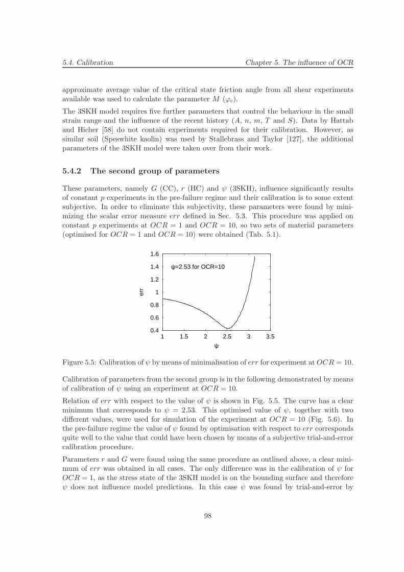
5.4. Calibration Chapter 5. The influence of OCR
approximate average value of the critical state friction angle from all shear experimentsavailable was used to calculate the parameter M (ϕc).
The 3SKH model requires five further parameters that control the behaviour in the smallstrain range and the influence of the recent history (A, n, m, T and S). Data by Hattaband Hicher [58] do not contain experiments required for their calibration. However, assimilar soil (Speswhite kaolin) was used by Stallebrass and Taylor [127], the additionalparameters of the 3SKH model were taken over from their work.
5.4.2 The second group of parameters
These parameters, namely G (CC), r (HC) and ψ (3SKH), influence significantly resultsof constant p experiments in the pre-failure regime and their calibration is to some extentsubjective. In order to eliminate this subjectivity, these parameters were found by mini-mizing the scalar error measure err defined in Sec. 5.3. This procedure was applied onconstant p experiments at OCR = 1 and OCR = 10, so two sets of material parameters(optimised for OCR = 1 and OCR = 10) were obtained (Tab. 5.1).
0.4
0.6
0.8
1
1.2
1.4
1.6
1 1.5 2 2.5 3 3.5
err
ψ
ψ=2.53 for OCR=10
Figure 5.5: Calibration of ψ by means of minimalisation of err for experiment atOCR = 10.
Calibration of parameters from the second group is in the following demonstrated by meansof calibration of ψ using an experiment at OCR = 10.
Relation of err with respect to the value of ψ is shown in Fig. 5.5. The curve has a clearminimum that corresponds to ψ = 2.53. This optimised value of ψ, together with twodifferent values, were used for simulation of the experiment at OCR = 10 (Fig. 5.6). Inthe pre-failure regime the value of ψ found by optimisation with respect to err correspondsquite well to the value that could have been chosen by means of a subjective trial-and-errorcalibration procedure.
Parameters r and G were found using the same procedure as outlined above, a clear mini-mum of err was obtained in all cases. The only difference was in the calibration of ψ forOCR = 1, as the stress state of the 3SKH model is on the bounding surface and thereforeψ does not influence model predictions. In this case ψ was found by trial-and-error by
98

5.5. Performance of the models Chapter 5. The influence of OCR
0
40
80
120
160
-0.06 -0.04 -0.02 0
q [k
Pa]
εv [-]0 0.02 0.04 0.06 0.08 0.1
εs [-]
experimentψ=2
ψ=2.53ψ=3
Figure 5.6: Predictions of the test OCR=10 by the 3SKH model with err-optimised (ψ =2.53) and two different values of ψ.
simulation of the isotropic unloading test from Fig. 5.4.
Table 5.1: Material parameters
M , ϕc λ∗ κ∗ N
CC 1.1 0.065 0.0175 0.918HC 27.5◦ 0.065 0.01 0.9183SKH 1.1 0.065 0.0034 0.918
A n m T S
3SKH 1964 0.65 0.2 0.25 0.08
G, r, ψ (OCR1) G, r, ψ (OCR10)
CC 7330 kPa 2210 kPaHC 1.43 0.673SKH 2.3 2.53
5.5 Performance of the models
The two sets of parameters found in Sec. 5.4 were used in simulating experiments atthe whole range of OCRs. The initial states of p′, q and e measured in the experimentswere used in the simulations. In addition, the 3SKH model requires to specify the initialpositions of kinematic surfaces. These were aligned to reflect the stress history followed inthe experiments (Sec. 5.1).
The obtained scalar error measure err is plotted with respect to OCR in Fig. 5.7. From
99

5.5. Performance of the models Chapter 5. The influence of OCR
0.25
0.5
0.75
1
1.25
1.5
1.75
50 20 10 5 2 1
err
OCR
Parameters for OCR 10
0.5
0.75
1
1.25
1.5
1.75
2
err
Parameters for OCR 1
CCHC
3SKH
Figure 5.7: err for parameters optimised for OCR = 1 (top) and OCR = 10 (bottom).
this figure it appears that studied elasto-plastic and hypoplastic models have differentranges of validity of different sets of material parameters:
1. Hypoplastic (HC) model performs for higher OCRs less correctly than other twomodels when calibrated using data for OCR = 1. However, when calibrated athigher OCR, it produces the best predictions out of all tested models for the entirerange of OCRs, with more-or-less constant value of err.
2. Elasto-plastic (CC and 3SKH) models calibrated at OCR = 10 perform relativelycorrectly up to OCR ≈ 4. For lower OCRs parameters for normally consolidatedstate lead to better predictions, but in the case of 3SKH still worst than predictionsby hypoplasticity.
By definition, the value of err characterises model predictions in the pre-failure regime only.In order to evaluate predictions at failure, observed and predicted peak friction angles ϕpwere plotted with respect to OCR. The results were similar for both sets of parameters, Fig.5.8 shows them for parameters optimised for OCR = 10. HC and 3SKH models predict
100

5.5. Performance of the models Chapter 5. The influence of OCR
20
25
30
35
40
45
50
55
60
50 20 10 5 2 1
ϕ p [°
]
OCR
experimentCCHC
3SKH
Figure 5.8: Peak friction angles ϕp predicted by the models with parameters optimised forOCR = 10.
peak friction angles relatively accurately (HC is more accurate for OCR ≤ 10, 3SKH forOCR ≥ 20). CC model overestimates significantly ϕp for all states with OCR > 2. Thisis a well-known shortcoming of the CC model, caused by the elliptical shape of the yieldsurface.
While err gives a convenient quantitative measure of the model performance, it does notspecify the source of the prediction error. For qualitative comparison, the stress pathsnormalised by the Hvorslev equivalent pressure p∗e are plotted for OCR = 10 optimisedparameters in Fig. 5.9a. Overprediction of ϕp by the CC model is clear, the shape of thenormalised stress paths is predicted relatively correctly by both HC and 3SKH models.All models, however, overestimate dilation. Normalised stress paths of all models headtowards a unique critical state point, which has not been reached in the experiments athigher OCRs (Fig. 5.9a top). A possible reason may be in localisation of deformation inshear bands at higher OCRs.
q vs. ǫs graphs for OCR = 10 optimised parameters are shown in Fig. 5.9b. It is clear thathigher errors for low OCRs of elasto-plastic models, reflected in Fig. 5.7, are caused bythe underestimation of the shear stiffness in the case of CC and overestimation of the shearstiffness in the case of 3SKH (with the exception of OCR = 1). Low prediction errors bythe HC model (Fig. 5.7) are reflected also in qualitatively correct performance shown inFig. 5.9b. Volumetric changes shown in Fig. 5.10 reveal a general trend of overestimationof dilation for higher OCRs, as already discussed in the previous paragraph. The shapeof ǫv vs. ǫs curves is best predicted by the HC model. For high OCRs the 3SKH modelpredicts dilatant behaviour immediately after the start of the shear phase, which has notbeen observed in the experiments. On the other hand, hypoplasticity overestimates theinitial contraction for medium OCRs.
101

5.6. Concluding remarks Chapter 5. The influence of OCR
0
0.2
0.4
0.6
0 0.2 0.4 0.6 0.8 1
q/p e*
p/pe*
3SKH
0.2
0.4
0.6
q/p e*
HC
0.2
0.4
0.6
q/p e*
CC
0.7
0.6
0.4
0.2
q/p e*
experiment
(a)
0
200
400
600
800
1000
0 0.02 0.04 0.06 0.08 0.1 0.12 0.14
q [k
Pa]
εs [-]
3SKH
200
400
600
800
1000
q [k
Pa]
HC
200
400
600
800
1000
q [k
Pa]
CC
200
400
600
800
1000
1200
q [k
Pa]
experiment
(b)
Figure 5.9: Stress paths normalised by p∗e (a) and q vs. ǫs graphs (b) for OCR = 10optimised parameters.
5.6 Concluding remarks
Results of this study must be seen as preliminary, as only one set of experimental data onone particular soil was investigated. Presented results however show that at least two sets ofmaterial parameters should be considered for both hypoplastic and elasto-plastic models.It appears that the HC model requires a different set of material parameters only fornormally consolidated soil, a single set of parameters, which leads to accurate predictionsfor a broad range of OCRs, is sufficient for OCR > 1. Two sets of parameters should also
102

5.6. Concluding remarks Chapter 5. The influence of OCR
-0.08
-0.06
-0.04
-0.02
0
0.02
0.04
0 0.02 0.04 0.06 0.08 0.1 0.12 0.14
ε v [-
]
εs [-]
3SKH
-0.08
-0.06
-0.04
-0.02
0
0.02
0.04
ε v [-
]
HC
-0.08
-0.06
-0.04
-0.02
0
0.02
0.04
ε v [-
]
CC
-0.1
-0.08
-0.06
-0.04
-0.02
0
0.02
0.04
ε v [-
]
experiment
Figure 5.10: ǫv vs. ǫs graphs for OCR = 10 optimised parameters.
be used for studied elasto-plastic models, with the approximate limiting OCR ≈ 4.
It is perhaps not surprising that the two advanced models performed significantly betterthan the CC model in predicting the non-linear behaviour in the pre-failure regime andcorrectly estimating the peak friction angles for high OCRs. For higher OCRs the HCmodel leads to better predictions than the 3SKH, both from the point of view of the scalarerror measure err and a qualitative performance expressed by the stress - strain diagrams.Also, the 3SKH model can not be effectively calibrated to predict correctly the behaviourof soils in normally consolidated state.
103

Chapter 6
A hypoplastic constitutive modelfor clays with meta-stablestructure
6.1 Introduction
Constitutive modelling of natural structured clays has observed a notable development inpast years. The research is driven by need for suitable design procedures, which would allowa practising engineer to perform analyses which are reliable and safe, but still sufficientlycheap. Apart from the accuracy in reproducing the soil behaviour, the model used for thispurpose should be easy to calibrate on the basis of laboratory experiments performed in astandard experimental equipment available in practice. The main objective of the researchpresented in this paper is to provide an advanced constitutive model for structured claysthat fulfills these requirements.
Most of the currently available constitutive models, which describe the destructuration pro-cesses in natural clays are developed within the framework of elasto-plasticity and visco-plasticity and may be seen as different extensions of the classical critical state model,developed at Cambridge University in 1960’s [117]. This model is usually modified byincorporating the second hardening law, which describes the progressive changes of struc-ture of natural clay. The most simple models (such as the model by Liu and Carter [82])do not assume any other alteration of the original model, Wheeler et al. [145] includeanisotropic effects by modifying the shape of the state boundary surface. These models,however, are not capable of predicting non-linearity of behaviour of overconsolidated soils.This shortcoming is overcome by more advanced models that make use of the kinematichardening plasticity [103], such as models from References [8, 118, 71, 46]. Different ap-proaches to treat the behaviour of structured soils include the multilaminate framework[37], visco-plasticity [116], and super/subloading yield surface approach [5]. A commonfeature of these models is that the improvement in accuracy of predictions is often paid
104
6.2. Reference model Chapter 6. Modelling meta-stable structure
by an increase of complexity of calibration procedures and mathematical formulation, thusreducing their suitability for application in a routine design.
In the text, the usual sign convention of soil mechanics (compression positive) is adoptedthroughout. In line with the Terzaghi principle of effective stress, all stresses are effectivestresses. Common tensor notation (see, e.g., Reference [97]) is used.
6.2 Reference constitutive model
The theory of hypoplasticity [75, 77], developed independently at Universities of Karlsruheand Grenoble (see [133]), was in the past applied successfully in the development of con-stitutive relations for granular materials [53, 141, 29]. More recently, the research focusedon the development of hypoplastic constitutive models for fine-grained soils [105, 54, 61]).Masın [87] proposed a new hypoplastic constitutive model for clays, which combines math-ematical structure of hypoplastic models with the basic principles of the critical state soilmechanics and the Modified Cam clay model. Predictive capabilities of this model, com-pared with other advanced constitutive models, have been demonstrated, e.g., in References[99, 56]. The hypoplastic model for clays will be used as a reference model for the proposedmodification.
The rate formulation of hypoplastic models is, in general [80], characterised by a singleequation [53]1
σ = fsL : ǫ + fsfdN ‖ǫ‖ (6.1)
where L and N are fourth- and second-order constitutive tensors respectively, fs is barotropyfactor that incorporates the influence of the mean stress and fd is a pyknotropy factor, whichcontrols the influence of the relative density (overconsolidation ratio). Cauchy stress σ andvoid ratio e are considered as state variables. Complete mathematical formulation of thereference model is given in Appendix.
The model requires five material parameters, namely ϕc, N , λ∗, κ∗ and r. ϕc is the criticalstate friction angle. Parameters N and λ∗ define the position and shape of the isotropicvirgin compression line with the formulation according to Butterfield [18]:
ln(1 + e) = N − λ∗ ln
(
p
pr
)
(6.2)
where pr is the reference stress 1kPa. The parameter κ∗ determines bulk modulus atoverconsolidated states and the parameter r controls shear modulus. Although directcalibration of parameters κ∗ and r is possible [87], it is suggested to determine their valuesby means of parametric studies.
1To be more precise, the rate formulation of hypoplastic models reads σ = fsL : D+ fsfdN ‖D‖, whereσ is the objective stress rate and D the Euler’s stretching tensor. See, e.g., References [78, 14] for details.
105

6.3. Conceptual approach Chapter 6. Modelling meta-stable structure
6.3 Conceptual approach for incorporation of structure ef-fects into constitutive models
A conceptual framework for the behaviour of structured fine-grained soils was presentedby Cotecchia and Chandler [34]. They demonstrated that the influence of structure infine-grained soils can be quantified by the different sizes of the state boundary surfaces2 ofthe structured and reference materials (Fig. 6.1), where as the reference material is usuallyconsidered soil reconstituted under standard conditions [17]. Cotecchia and Chandler [34]show that assuming a geometric similarity between the state boundary surfaces of natu-ral and reference materials appears to be a reasonable approximation, although stronglyanisotropic natural soils may exhibit SBS which is not symmetric about the isotropic axis.
Figure 6.1: Framework for structured fine-grained materials (Cotecchia and Chandler 2000)
These observations are, in principle, applied in most of the currently available constitutivemodels for structured soils. In general, at least one additional state variable describing theeffects of structure is needed, namely the ratio of sizes of SBSs of natural and referencematerials, referred to as ’sensitivity’ (s). s represents natural fabric and degree of bondingbetween soil particles. The limit value usually characterise the reference soil (s = 1),although higher values may be reasonable for soils with ’stable’ elements of structure causedby natural fabric [8]. s is usually considered as a function of accumulated plastic strain.
2State boundary surface (SBS) is defined as a boundary of all possible states of a soil element in thestress-void ratio space.
106

6.4. Structure effects in hypoplasticity Chapter 6. Modelling meta-stable structure
6.4 Incorporation of structure effects into hypoplasticity
As opposed to the most elasto-plastic models, the mathematical formulation of hypoplasticmodels does not include explicitly the state boundary surface. However, Masın and Herle[97] demonstrated that the model formulation allows us to derive an expression for theso-called swept-out-memory (SOM) surface, which is a close approximation of the stateboundary surface.
They have shown that for any permitted stress state it is possible to calculate explicitlythe value of the pyknotropy factor fd on the swept-out-memory surface:
fd = ‖fsA−1 : N‖−1 (6.3)
where the fourth-order tensor A is expressed as
A = fsL − 1
λ∗σ ⊗ 1 (6.4)
Equations (6.3) and (6.31) can be combined to find the expression for the Hvorslev equiv-alent pressure p∗e for a given stress state σ on the swept-out-memory surface and thus todetermine the shape of the SOM surface in the normalised space σ/p∗e:
p∗e = 2p‖fsA−1 : N‖1/α (6.5)
where the Hvorslev equivalent pressure p∗e on the isotropic normal compression line isdefined as (from (6.2), Fig. 6.2)
p∗e = pr exp
[
N − ln(1 + e)
λ∗
]
(6.6)
Since the swept-out-memory surface is not given a priori, its shape is dependent on themodel parameters, namely ϕc and the ratio κ∗/λ∗. For parameters typical to fine-grainedsoils its shape is similar to the state boundary surface of the Modified Cam clay model (seeFig. 6.3 for different parameter sets).
As summarised in the Introduction, constitutive modelling of structured soils using theframework of elasto-plasticity has recently undergone a notable development. Only few at-tempts, however, have been made to incorporate structure effects into hypoplastic models.Bauer and Wu [12, 13] enhanced the early version of the hypoplastic model for granularmaterials [149], which considers Cauchy stress σ the only state variable, by the so-calledstructure tensor S. The Cauchy stress σ is in the model replaced by the ”transformedstress tensor” σt, defined as
σt = σ + S (6.7)
This transformation shifts the limit state locus in the stress space, thus enabling mod-elling the cohesive behaviour of cemented materials. A suitable evolution equation for thestructure tensor S then allows us to simulate degradation of cementation bonds.
107

6.4. Structure effects in hypoplasticity Chapter 6. Modelling meta-stable structure
*λ
*κ
s=1SBS for
ln s1
*λ
ln ppe* pe
*s
N
current state
Isot. unl.
eln (1+ )
Current SBS, nat.1
ln s
Figure 6.2: On definitions of the sensitivity s, Hvorslev equivalent pressure p∗e and materialparameters N , λ∗ and κ∗.
A different approach for incorporating the structure effects into hypoplastic model is pro-posed in the present work. Soil with stable structure (constant sensitivity) is consideredfirst, following Ingram [65]. As in the present work sensitivity s is measured along constantvolume sections through the state boundary surfaces (Fig. 6.2), the Hvorslev equivalentpressure of the structured material is calculated by sp∗e (Fig. 6.2). It follows from theexpression of the SOM surface (Eqs. (6.3)-(6.6)) that the reference hypoplastic model maybe modified for clays with stable structure by a simple replacement of p∗e in the expressionfor fd (see Eq. (6.31) in Appendix) by sp∗e:
fd =
(
2p
sp∗e
)α
(6.8)
Eq. (6.8) causes that the SBS of a natural soil is s times larger than the SBS of a cor-responding reference material. It also follows from Fig. 6.2 that the normal compressionline of a natural soil is shifted along ln(1 + e) axis in the ln(1 + e) vs. ln p space by λ∗ ln s.Additional enhancement by the transformed stress tensor σt (6.7) would shift the SBSalong the isotropic axis and thus would allow us to model true cohesive behaviour due tocementation bonds [89]. For simplicity, the latter modification is omitted in this Note.
Second, the model is modified to predict the structure degradation. The proposed evolutionequation for sensitivity s reads (similarly to Baudet and Stallebrass [8])
s = − k
λ∗(s− sf )ǫ
d (6.9)
where k is a constitutive parameter that controls the rate of the structure degradation andsf is the final sensitivity. The damage strain ǫd is defined by
ǫd =
√
(ǫv)2 +
A
1 −A(ǫs)
2 (6.10)
108

6.4. Structure effects in hypoplasticity Chapter 6. Modelling meta-stable structure
-0.4
-0.2
0
0.2
0.4
0.6
0 0.2 0.4 0.6 0.8 1
q/p* e
p/p*e
London clayBeaucaire marl
Pisa clayBotkennar clay
Kaolin clay
Figure 6.3: SOM surface of the hypoplastic model for clays for five different sets of materialparameters (London clay – Masın 2005; Beaucaire marl – Masın et al. 2006; Kaolin – Hajekand Masın 2006; Bothkennar and Pisa clay – this study.).
with the parameter A, which controls the relative importance of the volumetric and shearcomponents (similarly to Rouiania and Wood [118]). Obviously, Eq. (6.10) does not allowmodelling purely deviatoric structure degradation process (A → 1). Nevertheless, theresearch in References [118, 46, 23] indicate that the value of the parameter A may be formost clays expected in the range (0 < A < 0.5).
In order to incorporate the variable sensitivity into the hypoplastic model, the barotropyfactor fs needs to be modified to ensure consistency between the model predictions and thestructure degradation law (6.9). Formulation of the model for the isotropic compressionfrom the isotropic normally compressed state is given by
p = −[
1
3 (1 + e)fs
(
3 + a2 − 2αa√
3)
]
e (6.11)
The isotropic normal compression line of the model incorporating structure reads (see Fig.6.2)
ln(1 + e) = N + λ∗ ln s− λ∗ ln
(
p
pr
)
(6.12)
Time differentiation of (6.12) results in
e
1 + e= λ∗
(
s
s− p
p
)
(6.13)
The isotropic formulation of the structure degradation law (6.9-6.10) is
s =k
λ∗(s − sf )
e
1 + e(6.14)
Combination of (6.13) and (6.14) yields
p
p= −
[
s− k(s− sf )
λ∗s
]
e
1 + e(6.15)
109

6.4. Structure effects in hypoplasticity Chapter 6. Modelling meta-stable structure
which may be compared with (6.11) to find an expression for the barotropy factor fs of thenew hypoplastic model:
fs = Si3p
λ∗
(
3 + a2 − 2αa√
3)−1
(6.16)
with the factor
Si =s− k(s− sf )
s(6.17)
Thus the factor fs of the modified model reads fs = Sifsr, where fsr is the barotropy factorof the reference model (see Eq. (6.30) in Appendix).
It follows from (6.1) that the factor fs controls the directional tangential stiffness of material(in terms of response envelopes [50] it controls their size). Therefore, the decrease of thestiffness in isotropic compression to ensure consistency with the structure degradationlaw (Eqs. (6.11)-(6.17)) has an undesired effect that also shear stiffness (controlled byparameter r) and stiffness in isotropic unloading (controlled by parameter κ∗) is decreased,see Fig. 6.4 (case A). Manipulation with the model reveals that the physical meaning ofthe parameters r and κ∗ is retained if they are both scaled by the factor Si (Fig. 6.4, caseB). Therefore, modification of scalar factors c1 (6.23) and α (6.24) is required. They nowread
c1 =2(
3 + a2 − 2αa√
3)
9rSiα =
1
ln 2ln
[
λ∗ − κ∗Siλ∗ + κ∗Si
(
3 + a2
a√
3
)]
(6.18)
50
60
70
80
90
100
110
70 80 90 100 110 120 130 140 150
σ 1 [k
Pa]
σ2 √2 [kPa]
Si=1case Acase B
Figure 6.4: Response envelopes of the model with constant sensitivity (Si = 1), modelmodified only by multiplication of the factor fs by Si (case A) and model where thephysical meaning of parameters r and κ∗ is retained (case B).
Equations (6.8–6.10), (6.16–6.17) and (6.18) are the only modifications of the referencehypoplastic model. The new model assumes one additional state variable s and threeadditional parameters: k, A, and sf . Their calibration procedure is detailed in the followingtext.
110

6.5. Model performance and calibration Chapter 6. Modelling meta-stable structure
6.5 Model performance and calibration
The performance of the proposed hypoplastic model will be evaluated using the conceptof the normalised incremental stress response envelopes (NIREs, see Fig. 6.5). They havebeen introduced by Masın and Herle [97] and follow directly from the concept of incrementalresponse envelopes [134] and rate response envelopes [50].
∆ε r2
∆ε a
p/p*e
q/p*e
R∆ε
Figure 6.5: Demonstration of the normalised incremental stress response envelopes foraxisymmetric conditions.
Figures 6.6a and 6.6b show the NIREs for different R∆ǫ = ‖∆ǫ‖ for natural and reconsti-tuted specimens of Pisa clay (see the next section), with symbols for isotropic and constantvolume loading and unloading. For small R∆ǫ (states well inside the swept-out-memorysurface, Fig. 6.6a) the NIREs of the natural and reconstituted clays are similar in shape,the sizes of the NIREs of the natural clay are s0 times larger than corresponding NIREsof the reconstituted clay (where s0 is the initial sensitivity of the natural clay). We seethat although the damage strain (6.10) is defined in terms of total strain rates (insteadof plastic strain rates as usual in elasto-plastic models), the model predicts only minorstructure degradation for states inside the SBS. Minor structure degradation also insidethe SBS is supported by Takahashi et al. [128].
For larger R∆ǫ (Fig. 6.6b) the NIREs of the reconstituted clay coincide with its swept-out-memory surface. The progressive structure degradation of the natural clay, however,causes the NIREs of the natural clay to shrink towards the swept-out-memory surfaceof the reconstituted material. The heart-like shape of the NIREs of the natural clay forR∆ǫ > 8% is caused by the low value of the parameter A (Tab. 6.1), which causes moresignificant influence of the volumetric strain component on the structure degradation.
The influence of the parameter k on model predictions is demonstrated in Fig. 6.7a. Thevalue of the parameter k was varied, while other model parameters (Tab. 6.1) were keptunchanged. The figure demonstrates the faster structure degradation for larger values ofthe parameter k. The influence of the parameter A is shown in Fig. 6.7b. Larger value ofthe parameter A increases the influence of shear strains on the structure degradation andthus flattens the NIREs. The common point of all NIREs is at the isotropic stress state.
111

6.5. Model performance and calibration Chapter 6. Modelling meta-stable structure
-1.5
-1
-0.5
0
0.5
1
1.5
2
0 0.5 1 1.5 2 2.5 3 3.5
q/p* e
p/p*e
2%1%0.5%
0.25%
SOMS rec.
SOMS nat.
init. nat.
init. rec.
reconst.natural
(a)
-1.5
-1
-0.5
0
0.5
1
1.5
2
0 0.5 1 1.5 2 2.5 3 3.5
q/p* e
p/p*e
4%8%16%32%
SOMS rec.
SOMS nat.
init. nat.
init. rec.
reconst.natural
(b)
Figure 6.6: Normalised incremental stress response envelopes of the proposed hypoplasticmodel plotted for medium (a) and large (b) strain range (R∆ǫ is indicated). The envelopesfor the reconstituted material obtained with the reference hypoplastic model (Masın 2005)are also included.
Therefore, the parameter k may be calibrated independently of the parameter A on thebasis of an isotropic compression test on natural soil. The parameter A is calibrated withthe already known value of k using an experiment where significant shear strains develop.
-1.5
-1
-0.5
0
0.5
1
1.5
2
0 0.5 1 1.5 2 2.5 3 3.5
q/p* e
p/p*e
SOMS rec.
SOMS nat.
init. nat.
init. rec.k=0.1
k=0.4
k=0.7
k=1
||∆ε||=8%
(a)
-1.5
-1
-0.5
0
0.5
1
1.5
2
0 0.5 1 1.5 2 2.5 3 3.5
q/p* e
p/p*e
SOMS rec.
SOMS nat.
init. nat.
init. rec.
||∆ε||=8%
A=0.1A=0.3A=0.5A=0.7A=0.9
(b)
Figure 6.7: The influence of the parameter k (a) and A (b).
The initial value of sensitivity may be determined from an assumption of a geometricsimilarity between SBSs of natural and reconstituted soil [34] as a ratio of undrainedshear strengths of natural and reconstituted soil, or as a ratio of stresses at gross yield incompression tests (e.g., K0 or isotropic) on natural specimens and equivalent stresses atcorresponding normal compression lines of a reconstituted soil. The final value of sensitivitysf may be derived from compression tests on natural and reference materials performed to
112

6.6. Evaluation of model predictions Chapter 6. Modelling meta-stable structure
very large strains [7].
6.6 Evaluation of model predictions
The proposed model will be evaluated on the basis of laboratory experiments on two naturalclays with meta-stable structure.
Callisto and Calabresi [20] reported laboratory experiments on natural Pisa clay. Drainedprobing tests were performed, with rectilinear stress paths having different orientations inthe stress space. In addition to the tests on natural Pisa clay, experiments with the samestress paths were performed on reconstituted clay. Tests are labelled by prefix ’A’ and ’R’for natural and reconstituted clay respectively, followed by the angle of stress paths in theq : p space (measured in degrees anti-clockwise from the isotropic loading direction).
All the parameters of the proposed hypoplastic model, with the exception of parametersrelated to the effects of structure (k, A and sf ), were be calibrated solely using laboratoryexperiments on the reconstituted Pisa clay. The parameters N , λ∗ and κ∗ were calibratedon the basis of an isotropic compression test on reconstituted Pisa clay ([19], Fig. 6.8a).Critical state friction angle ϕc has been found by evaluating the data from shear tests,parameter r has been calibrated on the basis of a parametric study using a single sheartest (R60, Fig. 6.8b).
0.6
0.65
0.7
0.75
0.8
0.85
0.9
3.5 4 4.5 5 5.5 6 6.5
ln (
1+e)
[-]
ln (p/pr) [-]
Isotr. NCLexperiment
κ*=0.005κ*=0.0075
κ*=0.010κ*=0.015
(a)
0.4
0.45
0.5
0.55
0.6
0.65
0.7
0.75
0.8
0 0.05 0.1 0.15 0.2
q/p
[-]
εs [-]
R60r=0.1r=0.3r=0.5
(b)
Figure 6.8: Calibration of the parameters N , λ∗ and κ∗ on the basis of an isotropic com-pression test on reconstituted Pisa clay (a), parametric study for the calibration of theparameter r (b).
For the calibration of the structure-related parameters k, A and sf , it has been assumed,following Callisto and Rampello [23], that the experimental procedures adopted for prepa-ration of reconstituted specimens reproduced correctly the stress history of the Pisa claydeposit. Therefore, the stress paths of the equivalent experiments on natural and reconsti-tuted clays should coincide, when plotted in the space normalised with respect to volume
113

6.6. Evaluation of model predictions Chapter 6. Modelling meta-stable structure
and structure σ/(p∗es) [34]. The current value of sensitivity s may be found by the time-integration of the structure degradation law (6.9-6.10):
s = sf + (s0 − sf ) exp
[
− k
λ∗ǫd]
(6.19)
where ǫd is the accumulated damage strain
ǫd =
∫ t1
t0
ǫddt (6.20)
In this way, parameters k and A (and the initial value of sensitivity s) could be calibrateddirectly by evaluation of the experimental data, without reference to single element mod-elling of tests on natural clay. Calibration of the parameter k is demonstrated in Fig. 6.9a.The shear strains in the test A0 are negligible, thus the parameter A does not influencepredictions of the structure degradation process (Fig. 6.7b, Eq. (6.10)). The value of theparameter A was calibrated with the already known value of the parameter k using resultsfrom shear tests R90 and A90 (Fig. 6.9b). The final value of sensitivity sf is assumed to beequal to one. This appears to be a reasonable approximation [7], although no compressionor shear experiment on natural clay which would lead to a full destructuration is available.Parameters of the hypoplastic model for natural Pisa clay are summarised in Table 6.1 andthe initial values of state variables in Table 6.2.
Table 6.1: Parameters of the proposed hypoplastic model for Pisa clay and Bothkennar
clay.
ϕc λ∗ κ∗ N r k A sfPisa 21.9◦ 0.14 0.0075 1.56 0.3 0.4 0.1 1
Bothkennar 35◦ 0.119 0.003 1.344 0.07 0.35 0.5 1
Table 6.2: The initial values of the state variables for natural and reconstituted Pisa clay
and natural Bothkennar clay.
p [kPa] q [kPa] e reconst. e nat. s
88.2 38 1.302 1.738 3.4534 18 – 1.88 6
The evaluated parameters were used for simulation of laboratory experiments on Pisaclay. Experimental data compared with predictions by the proposed hypoplastic modelare shown in Figs. 6.10, 6.11 and 6.12. The figures show that the hypoplastic model,due to its non-linear nature, predicts correctly the gradual change of stiffness as the statemoves towards the state boundary surface. Consequently, the model predicts in agreement
114
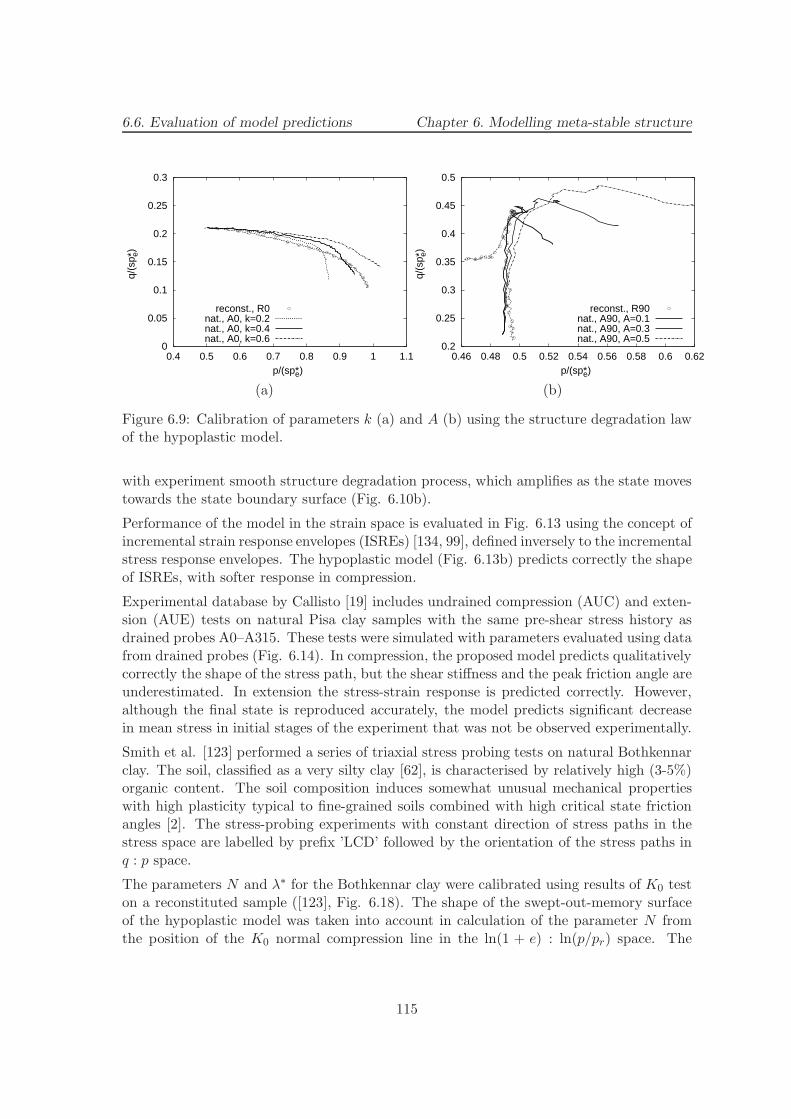
6.6. Evaluation of model predictions Chapter 6. Modelling meta-stable structure
0
0.05
0.1
0.15
0.2
0.25
0.3
0.4 0.5 0.6 0.7 0.8 0.9 1 1.1
q/(s
p* e)
p/(sp*e)
reconst., R0nat., A0, k=0.2nat., A0, k=0.4nat., A0, k=0.6
(a)
0.2
0.25
0.3
0.35
0.4
0.45
0.5
0.46 0.48 0.5 0.52 0.54 0.56 0.58 0.6 0.62
q/(s
p* e)
p/(sp*e)
reconst., R90nat., A90, A=0.1nat., A90, A=0.3nat., A90, A=0.5
(b)
Figure 6.9: Calibration of parameters k (a) and A (b) using the structure degradation lawof the hypoplastic model.
with experiment smooth structure degradation process, which amplifies as the state movestowards the state boundary surface (Fig. 6.10b).
Performance of the model in the strain space is evaluated in Fig. 6.13 using the concept ofincremental strain response envelopes (ISREs) [134, 99], defined inversely to the incrementalstress response envelopes. The hypoplastic model (Fig. 6.13b) predicts correctly the shapeof ISREs, with softer response in compression.
Experimental database by Callisto [19] includes undrained compression (AUC) and exten-sion (AUE) tests on natural Pisa clay samples with the same pre-shear stress history asdrained probes A0–A315. These tests were simulated with parameters evaluated using datafrom drained probes (Fig. 6.14). In compression, the proposed model predicts qualitativelycorrectly the shape of the stress path, but the shear stiffness and the peak friction angle areunderestimated. In extension the stress-strain response is predicted correctly. However,although the final state is reproduced accurately, the model predicts significant decreasein mean stress in initial stages of the experiment that was not be observed experimentally.
Smith et al. [123] performed a series of triaxial stress probing tests on natural Bothkennarclay. The soil, classified as a very silty clay [62], is characterised by relatively high (3-5%)organic content. The soil composition induces somewhat unusual mechanical propertieswith high plasticity typical to fine-grained soils combined with high critical state frictionangles [2]. The stress-probing experiments with constant direction of stress paths in thestress space are labelled by prefix ’LCD’ followed by the orientation of the stress paths inq : p space.
The parameters N and λ∗ for the Bothkennar clay were calibrated using results of K0 teston a reconstituted sample ([123], Fig. 6.18). The shape of the swept-out-memory surfaceof the hypoplastic model was taken into account in calculation of the parameter N fromthe position of the K0 normal compression line in the ln(1 + e) : ln(p/pr) space. The
115

6.6. Evaluation of model predictions Chapter 6. Modelling meta-stable structure
-1.5
-1
-0.5
0
0.5
1
1.5
2
0 0.5 1 1.5 2 2.5 3 3.5
q/p* e
p/p*e
A0
A30
A60A90A135
A180
A280 A315
R0
R315
R30R60R90
experiment, reconst.experiment, nat.
(a)
-1.5
-1
-0.5
0
0.5
1
1.5
2
0 0.5 1 1.5 2 2.5 3 3.5q/
p* ep/p*e
A0
A30A60
A90A135
A180
A280 A315
R0
R315
R30R60R90
SOMS rec.
SOMS nat.
hypo., reconst.hypo., nat.
(b)
Figure 6.10: Normalised stress paths of the natural and reconstituted Pisa clay (a) andpredictions by the hypoplastic model (b).
0.88
0.9
0.92
0.94
0.96
0.98
1
1.02
1.04
1.06
2.5 3 3.5 4 4.5 5 5.5 6
ln(1
+e)
[-]
ln(p/pr) [-]
A0
A30
A60
A90
A135A180
A280
A315
Isot. NCL rec.experiment, nat.
(a)
0.88
0.9
0.92
0.94
0.96
0.98
1
1.02
1.04
1.06
2.5 3 3.5 4 4.5 5 5.5 6
ln(1
+e)
[-]
ln(p/pr) [-]
A0A30
A60
A90
A135A180
A280
A315Isot. NCL rec.hypo., nat.
(b)
Figure 6.11: Experiments on natural Pisa clay plotted in the ln(p/pr) vs. ln(1 + e) space(a) and predictions by the proposed hypoplastic model (b).
116

6.6. Evaluation of model predictions Chapter 6. Modelling meta-stable structure
-50
0
50
100
150
-0.05 0 0.05 0.1 0.15
q [k
Pa]
εs [-]
A0
A30 A60
A90A135
A180
A280
A315
experiment, nat.
(a)
-50
0
50
100
150
-0.05 0 0.05 0.1 0.15q
[kP
a]εs [-]
A0
A30
A60
A90A135
A180
A280
A315 hypo., nat.
(b)
Figure 6.12: ǫs vs. q diagrams of experiments on natural Pisa clay (a) and predictions bythe proposed hypoplastic model (b).
-0.005
0
0.005
0.01
0.015
0.02
-0.015 -0.01 -0.005 0 0.005 0.01
ε a [-
]
√2 εr [-]
experiment, nat.
A0
A30A60A90
A135
A180 A280 A315
(a)
-0.005
0
0.005
0.01
0.015
0.02
-0.015 -0.01 -0.005 0 0.005 0.01
ε a [-
]
√2 εr [-]
hypoplas., nat.
A0
A30A60
A90
A135
A180
A280
A315
(b)
Figure 6.13: Incremental strain response envelopes for R∆σ = ‖∆σ‖=10, 20, 30 (bro-ken line), 50 and 100 kPa, plotted together with strain paths in the
√2ǫr vs. ǫa space.
Experimental data on natural Pisa clay (a) and predictions by the hypoplastic model (b).
117
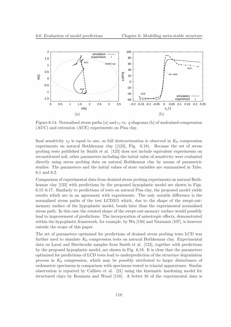
6.6. Evaluation of model predictions Chapter 6. Modelling meta-stable structure
-1.5
-1
-0.5
0
0.5
1
1.5
2
0 0.5 1 1.5 2 2.5 3 3.5
q/p* e
p/p*e
AUC
AUE
SOMS nat.
simulationexperiment
(a)
-60
-40
-20
0
20
40
60
80
100
-0.2 -0.15 -0.1 -0.05 0 0.05 0.1 0.15 0.2 0.25
q [k
Pa]
εs [-]
AUC
AUE
init. state
simulationexperiment
(b)
Figure 6.14: Normalised stress paths (a) and ǫs vs. q diagrams (b) of undrained compression(AUC) and extension (AUE) experiments on Pisa clay.
final sensitivity sf is equal to one, as full destructuration is observed in K0 compressionexperiments on natural Bothkennar clay ([123], Fig. 6.18). Because the set of stressprobing tests published by Smith et al. [123] does not include equivalent experiments onreconstituted soil, other parameters including the initial value of sensitivity were evaluateddirectly using stress probing data on natural Bothkennar clay by means of parametricstudies. The parameters and the initial values of state variables are summarised in Tabs.6.1 and 6.2.
Comparison of experimental data from drained stress probing experiments on natural Both-kennar clay [123] with predictions by the proposed hypoplastic model are shown in Figs.6.15–6.17. Similarly to predictions of tests on natural Pisa clay, the proposed model yieldsresults which are in an agreement with experiments. The only notable difference is thenormalised stress paths of the test LCD315 which, due to the shape of the swept-out-memory surface of the hypoplastic model, bends later than the experimental normalisedstress path. In this case the rotated shape of the swept-out-memory surface would possiblylead to improvement of predictions. The incorporation of anisotropic effects, demonstratedwithin the hypoplastic framework, for example, by Wu [150] and Niemunis [107], is howeveroutside the scope of this paper.
The set of parameters optimized for predictions of drained stress probing tests LCD wasfurther used to simulate K0 compression tests on natural Bothkennar clay. Experimentaldata on Laval and Sherbrooke samples from Smith et al. [123], together with predictionsby the proposed hypoplastic model, are shown in Fig. 6.18. It is clear that the parametersoptimized for predictions of LCD tests lead to underprediction of the structure degradationprocess in K0 compression, which may be possibly attributed to larger disturbance ofoedometric specimens in comparison with specimens tested in triaxial apparatuses. Similarobservation is reported by Callisto et al. [21] using the kinematic hardening model forstructured clays by Rouiania and Wood [118]. A better fit of the experimental data is
118

6.6. Evaluation of model predictions Chapter 6. Modelling meta-stable structure
-4
-3
-2
-1
0
1
2
3
4
5
0 1 2 3 4 5 6
q/p* e
p/p*e
SOMS hypo.
LCD0
LCD30
LCD55
LCD70LCD110
LCD180
LCD315
experiment
(a)
-4
-3
-2
-1
0
1
2
3
4
5
0 1 2 3 4 5 6q/
p* ep/p*e
SOMS
LCD0
LCD30
LCD55
LCD70LCD110
LCD180
LCD315
hypoplasticity
(b)
Figure 6.15: Normalised stress paths of the natural and reconstituted Bothkennar clay (a)and predictions by the proposed hypoplastic model (b).
0.9
0.95
1
1.05
1.1
2 2.5 3 3.5 4 4.5 5
ln(1
+e)
[-]
ln(p/pr) [-]
LCD0
LCD
30
LCD
55
LCD70
LCD110LCD180
LCD315
Isot. NCL rec.experiment
(a)
0.9
0.95
1
1.05
1.1
2 2.5 3 3.5 4 4.5 5
ln(1
+e)
[-]
ln(p/pr) [-]
LCD0LCD
30
LCD
55
LCD70
LCD110
LCD180
LCD315
Isot. NCL rec.hypoplasticity
(b)
Figure 6.16: Experiments on natural Bothkennar clay plotted in the ln(p/pr) vs. ln(1 + e)space (a) and predictions by the proposed hypoplastic model (b).
119
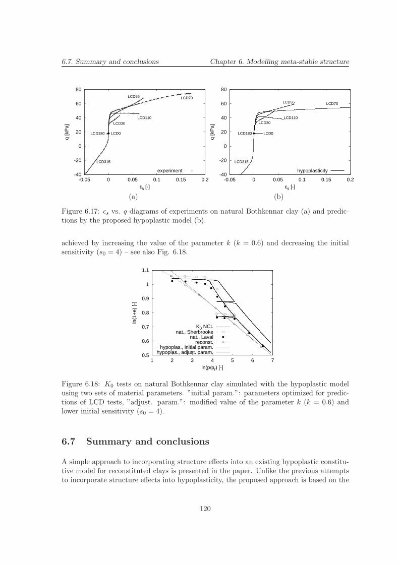
6.7. Summary and conclusions Chapter 6. Modelling meta-stable structure
-40
-20
0
20
40
60
80
-0.05 0 0.05 0.1 0.15 0.2
q [k
Pa]
εs [-]
LCD0
LCD30
LCD55 LCD70
LCD110
LCD180
LCD315
experiment
(a)
-40
-20
0
20
40
60
80
-0.05 0 0.05 0.1 0.15 0.2
q [k
Pa]
εs [-]
LCD0
LCD30
LCD55 LCD70
LCD110
LCD180
LCD315
hypoplasticity
(b)
Figure 6.17: ǫs vs. q diagrams of experiments on natural Bothkennar clay (a) and predic-tions by the proposed hypoplastic model (b).
achieved by increasing the value of the parameter k (k = 0.6) and decreasing the initialsensitivity (s0 = 4) – see also Fig. 6.18.
0.5
0.6
0.7
0.8
0.9
1
1.1
1 2 3 4 5 6 7
ln(1
+e)
[-]
ln(p/pr) [-]
K0 NCLnat., Sherbrooke
nat., Lavalreconst.
hypoplas., initial param.hypoplas., adjust. param.
Figure 6.18: K0 tests on natural Bothkennar clay simulated with the hypoplastic modelusing two sets of material parameters. ”initial param.”: parameters optimized for predic-tions of LCD tests, ”adjust. param.”: modified value of the parameter k (k = 0.6) andlower initial sensitivity (s0 = 4).
6.7 Summary and conclusions
A simple approach to incorporating structure effects into an existing hypoplastic constitu-tive model for reconstituted clays is presented in the paper. Unlike the previous attemptsto incorporate structure effects into hypoplasticity, the proposed approach is based on the
120

6.7. Summary and conclusions Chapter 6. Modelling meta-stable structure
modification of the barotropy and pyknotropy factors that leads to an increase of the sizeof the state boundary surface predicted by the model and ensures consistency between themodel predictions and the pre-defined structure degradation law. Model predictions com-pare well with experimental data on two natural clays. In fact, predictions of laboratoryexperiments on natural Pisa and Bothkennar clays presented in the paper are compara-ble with predictions by kinematic hardening elasto-plastic models, see [7, 21] for drainedprobing tests on natural Pisa clay and [8, 7, 46] for LCD tests on natural Bothkennar clay.
The proposed method for incorporating the structure effects into hypoplasticity also opensa way to model other structural effects using hypoplasticity theory, such as mechanical [79]and chemical [111] debonding in cemented granular materials, simulating grain crushing[25], or modelling unsaturated [3] and double-porosity materials [93].
Appendix
The mathematical formulation of a reference hypoplastic model for clays model is sum-marised briefly in the following. The rate formulation of the hypoplastic model reads
σ = fsL : ǫ + fsfdN ‖ǫ‖ (6.21)
The fourth-order tensor L is a hypoelastic tensor given by
L = 3(
c1I + c2a2σ ⊗ σ
)
(6.22)
with the two scalar factors c1 and c2 introduced by [61] and modified by [87]:
c1 =2(
3 + a2 − 2αa√
3)
9rc2 = 1 + (1 − c1)
3
a2(6.23)
where the scalars a and α are functions of the material parameters ϕc, λ∗ and κ∗
a =
√3 (3 − sinϕc)
2√
2 sinϕcα =
1
ln 2ln
[
λ∗ − κ∗
λ∗ + κ∗
(
3 + a2
a√
3
)]
(6.24)
The second-order tensor N is given by Niemunis [106]
N = L :
(
Ym
‖m‖
)
(6.25)
where the quantity Y determines the shape of the critical state locus in the stress spacesuch that for Y = 1 it coincides with the Matsuoka and Nakai [85] limit stress condition.
Y =
( √3a
3 + a2− 1
)
(I1I2 + 9I3)(
1 − sin2 ϕc)
8I3 sin2 ϕc+
√3a
3 + a2(6.26)
121

6.7. Summary and conclusions Chapter 6. Modelling meta-stable structure
with the stress invariants
I1 = tr(σ) I2 =1
2
[
σ : σ − (I1)2]
I3 = det(σ)
det(σ) is the determinant of σ. The second-order tensor m has parallel in the flow rule inelasto-plasticity. It is calculated by
m = − a
F
[
σ + dev σ − σ
3
(
6σ : σ − 1
(F/a)2 + σ : σ
)]
(6.27)
with the factor F
F =
√
1
8tan2 ψ +
2 − tan2 ψ
2 +√
2 tanψ cos 3θ− 1
2√
2tanψ (6.28)
where
tanψ =√
3 ‖dev σ‖ cos 3θ = −√
6tr (dev σ · dev σ · dev σ)
[dev σ : dev σ]3/2(6.29)
The barotropy factor fs introduces the influence of the mean stress level. The way of itsderivation ensures that the hypoplastic model predicts correctly the isotropic normallycompressed states.
fs =3p
λ∗
(
3 + a2 − 2αa√
3)−1
(6.30)
The pyknotropy factor fd incorporates the influence of the overconsolidation ratio. Thecritical state is characterised by fd = 1 and the isotropic normally compressed state byfd = 2α.
fd =
(
2p
p∗e
)α
p∗e = pr exp
[
N − ln(1 + e)
λ∗
]
(6.31)
with the reference stress pr = 1 kPa. Finally, evolution of the state variable e (void ratio)is governed by
e = − (1 + e) ǫv (6.32)
122

Chapter 7
Comparison of elasto-plastic andhypoplastic modelling ofstructured clays
7.1 Introduction
The recently developed constitutive models for structured clays are based on fundamentallydifferent mathematical backgrounds. The conceptual approach utilised for their develop-ment is, however, often very similar. These models are usually based on existing models forreconstituted soils with modified size (and in some cases also shape) of the state boundarysurface (SBS).
The aim of the paper is a further evaluation of a hypoplastic model for structured claysby Masın [88]. Predictions by this model are compared with its elasto-plastic alterna-tive developed in the paper. The Structured modified Cam clay (SMCC) model has asimilar structure degradation law and the same number of parameters with an equivalentphysical meaning as the hypoplastic model. Thus both models are characterised by thesame calibration procedure and the same complexity from the standpoint of a practisingengineer.
All simulations with the hypoplastic model are taken over from Reference [88]. The aim ofthe present work is to supplement these simulations by predictions of a simple elasto-plasticmodel and thus to reveal merits of the non-linear character of the hypoplastic formulation.
123
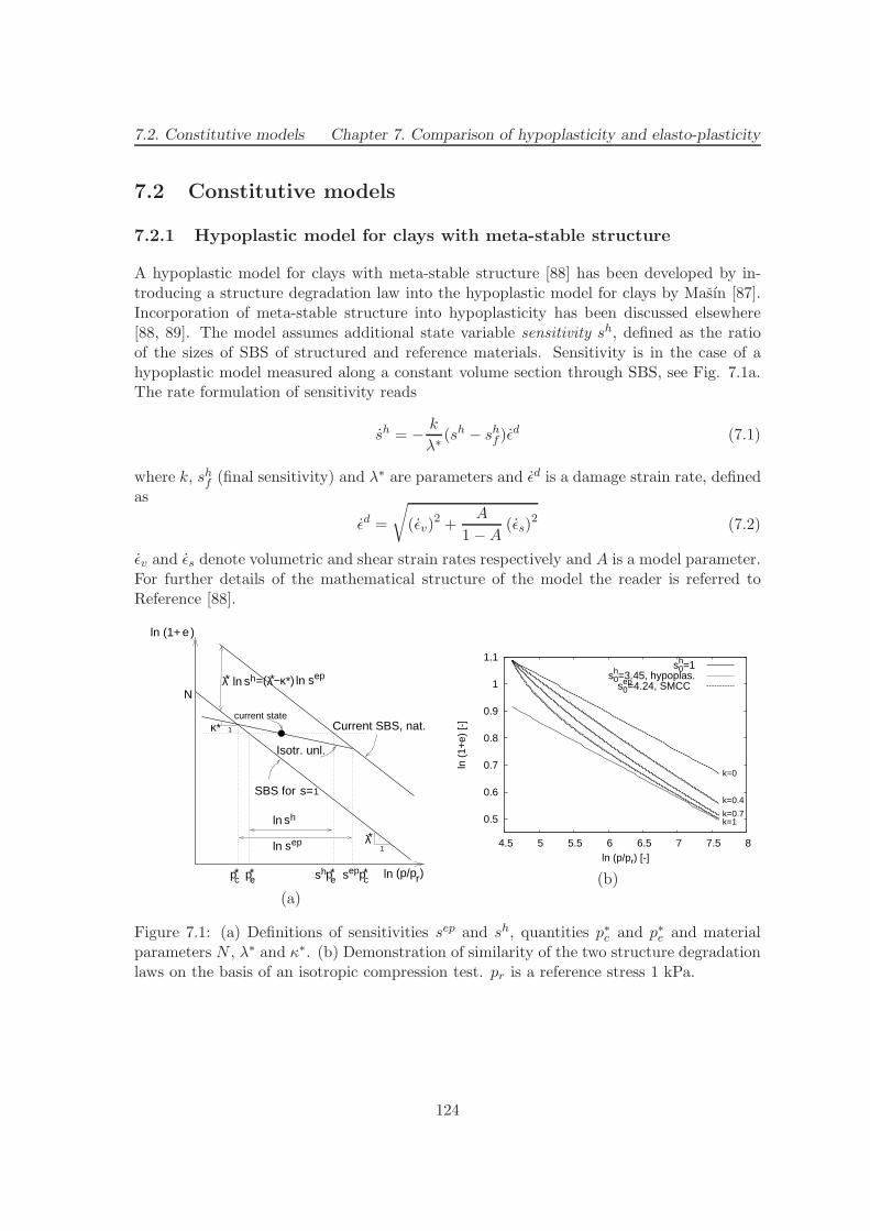
7.2. Constitutive models Chapter 7. Comparison of hypoplasticity and elasto-plasticity
7.2 Constitutive models
7.2.1 Hypoplastic model for clays with meta-stable structure
A hypoplastic model for clays with meta-stable structure [88] has been developed by in-troducing a structure degradation law into the hypoplastic model for clays by Masın [87].Incorporation of meta-stable structure into hypoplasticity has been discussed elsewhere[88, 89]. The model assumes additional state variable sensitivity sh, defined as the ratioof the sizes of SBS of structured and reference materials. Sensitivity is in the case of ahypoplastic model measured along a constant volume section through SBS, see Fig. 7.1a.The rate formulation of sensitivity reads
sh = − k
λ∗(sh − shf )ǫ
d (7.1)
where k, shf (final sensitivity) and λ∗ are parameters and ǫd is a damage strain rate, definedas
ǫd =
√
(ǫv)2 +
A
1 −A(ǫs)
2 (7.2)
ǫv and ǫs denote volumetric and shear strain rates respectively and A is a model parameter.For further details of the mathematical structure of the model the reader is referred toReference [88].
*λ
*λ
*κ
*κ*λ ln
s=1SBS for
c* pe
* pe* pc
*p s sh ep
ln
ln
s
sh
ep
ln (p/p )r
N
1
current state
eln (1+ )
Current SBS, nat.1
=( − ) sepln sh
Isotr. unl.
(a)
0.5
0.6
0.7
0.8
0.9
1
1.1
4.5 5 5.5 6 6.5 7 7.5 8
ln (
1+e)
[-]
ln (p/pr) [-]
k=0
k=0.4
k=0.7k=1
sh0=1
sh0=3.45, hypoplas.sep
0=4.24, SMCC
(b)
Figure 7.1: (a) Definitions of sensitivities sep and sh, quantities p∗c and p∗e and materialparameters N , λ∗ and κ∗. (b) Demonstration of similarity of the two structure degradationlaws on the basis of an isotropic compression test. pr is a reference stress 1 kPa.
124
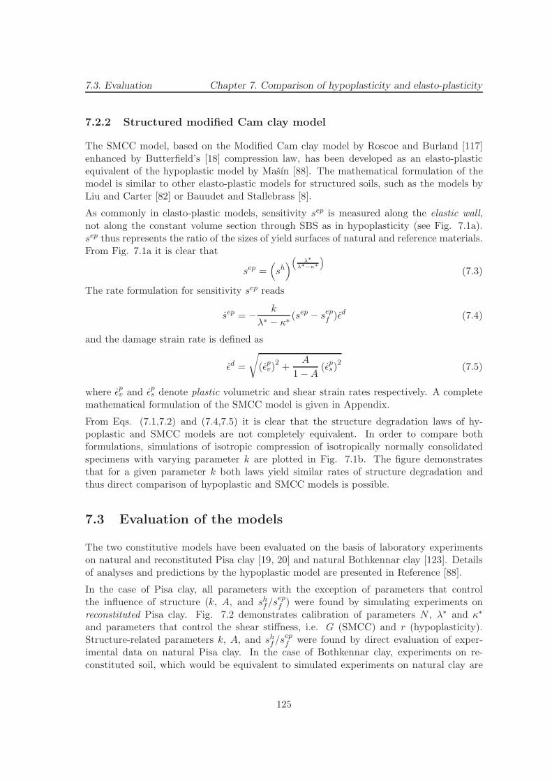
7.3. Evaluation Chapter 7. Comparison of hypoplasticity and elasto-plasticity
7.2.2 Structured modified Cam clay model
The SMCC model, based on the Modified Cam clay model by Roscoe and Burland [117]enhanced by Butterfield’s [18] compression law, has been developed as an elasto-plasticequivalent of the hypoplastic model by Masın [88]. The mathematical formulation of themodel is similar to other elasto-plastic models for structured soils, such as the models byLiu and Carter [82] or Bauudet and Stallebrass [8].
As commonly in elasto-plastic models, sensitivity sep is measured along the elastic wall,not along the constant volume section through SBS as in hypoplasticity (see Fig. 7.1a).sep thus represents the ratio of the sizes of yield surfaces of natural and reference materials.From Fig. 7.1a it is clear that
sep =(
sh)
“
λ∗
λ∗−κ∗
”
(7.3)
The rate formulation for sensitivity sep reads
sep = − k
λ∗ − κ∗(sep − sepf )ǫd (7.4)
and the damage strain rate is defined as
ǫd =
√
(ǫpv)2+
A
1 −A(ǫps)
2(7.5)
where ǫpv and ǫps denote plastic volumetric and shear strain rates respectively. A completemathematical formulation of the SMCC model is given in Appendix.
From Eqs. (7.1,7.2) and (7.4,7.5) it is clear that the structure degradation laws of hy-poplastic and SMCC models are not completely equivalent. In order to compare bothformulations, simulations of isotropic compression of isotropically normally consolidatedspecimens with varying parameter k are plotted in Fig. 7.1b. The figure demonstratesthat for a given parameter k both laws yield similar rates of structure degradation andthus direct comparison of hypoplastic and SMCC models is possible.
7.3 Evaluation of the models
The two constitutive models have been evaluated on the basis of laboratory experimentson natural and reconstituted Pisa clay [19, 20] and natural Bothkennar clay [123]. Detailsof analyses and predictions by the hypoplastic model are presented in Reference [88].
In the case of Pisa clay, all parameters with the exception of parameters that controlthe influence of structure (k, A, and shf/s
epf ) were found by simulating experiments on
reconstituted Pisa clay. Fig. 7.2 demonstrates calibration of parameters N , λ∗ and κ∗
and parameters that control the shear stiffness, i.e. G (SMCC) and r (hypoplasticity).Structure-related parameters k, A, and shf/s
epf were found by direct evaluation of exper-
imental data on natural Pisa clay. In the case of Bothkennar clay, experiments on re-constituted soil, which would be equivalent to simulated experiments on natural clay are
125

7.3. Evaluation Chapter 7. Comparison of hypoplasticity and elasto-plasticity
0.6
0.65
0.7
0.75
0.8
0.85
0.9
3.5 4 4.5 5 5.5 6 6.5
ln (
1+e)
[-]
ln (p/pr) [-]
Isotr. NCLexperiment
hypoplas., κ*=0.0075SMCC, κ*=0.020
(a)
0.4
0.45
0.5
0.55
0.6
0.65
0.7
0.75
0.8
0 0.05 0.1 0.15 0.2
q/p
[-]
εs [-]
R60hypoplas., r=0.3
SMCC, G=1 MPa
(b)
Figure 7.2: (a) Calibration of the parameters N , λ∗ and κ∗ of hypoplastic and SMCCmodels (isotropic compression test on reconstituted Pisa clay from Callisto 1996); (b)Calibration of the parameter r of the hypoplastic model and G of the SMCC model (datafrom Callisto and Calabresi 1998).
not available, thus all parameters were found by simulation of experiments on naturalBothkennar clay. Parameters of both models are summarised in Tab. 7.1.
Table 7.1: Parameters of the hypoplastic and SMCC models for Pisa and Bothkennar clays.
hypoplasticity ϕc λ∗ κ∗ N r k A shfPisa 21.9◦ 0.14 0.0075 1.56 0.3 0.4 0.1 1
Bothkennar 35◦ 0.119 0.003 1.344 0.07 0.35 0.5 1
SMCC M λ∗ κ∗ N G k A sepfPisa 0.85 0.14 0.02 1.56 1 MPa 0.4 0.1 1
Bothkennar 1.42 0.119 0.01 1.344 2 MPa 0.35 0.5 1
Fig. 7.3 shows results of simulations of experiments on Pisa clay, namely stress pathsnormalised by the Hvorslev equivalent pressure p∗e (a) and response in ln(p/pr) vs. ln(1+e)space (b). Normalised stress paths of natural Bothkennar clay are in Fig. 7.4a, ǫs vs. qcurves in Fig. 7.4b. Figures 7.3 and 7.4 demonstrate some common features and somedifferences in predictions by the hypoplastic and SMCC models. Both models predictapparently similar shape of the SBS and, in general, a similar stress-strain behaviour atlarger strains. The main difference stems from the non-linear character of the hypoplasticequation that facilitates the non-linear response also inside the SBS, with a gradual decreaseof shear and bulk moduli and a smooth structure-degradation process.
126
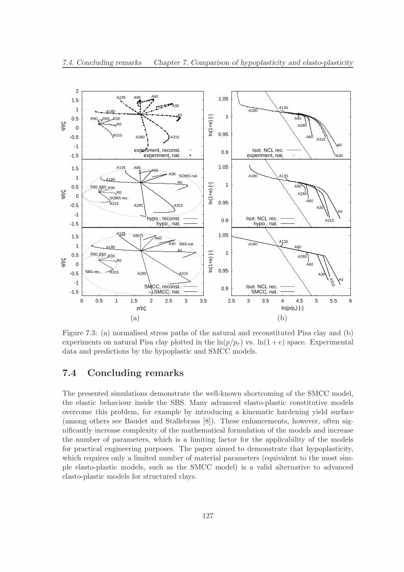
7.4. Concluding remarks Chapter 7. Comparison of hypoplasticity and elasto-plasticity
-1.5
-1
-0.5
0
0.5
1
1.5
0 0.5 1 1.5 2 2.5 3 3.5
q/p e*
p/pe*
A0
A30A60
A90A135
A180
A280 A315
R0
R315
R30R60R90
SBS rec.
SBS nat.
SMCC, reconst.SMCC, nat.
-1.5
-1
-0.5
0
0.5
1
1.5
q/p e*
A0
A30A60
A90A135
A180
A280 A315
R0
R315
R30R60R90
SOMS rec.
SOMS nat.
hypo., reconst.hypo., nat.
-1.5
-1
-0.5
0
0.5
1
1.5
2
q/p e*
A0
A30
A60A90A135
A180
A280 A315
R0
R315
R30R60R90
experiment, reconst.experiment, nat.
(a)
0.9
0.95
1
1.05
2.5 3 3.5 4 4.5 5 5.5 6
ln(1
+e)
[-]
ln(p/pr) [-]
A0A30
A60
A90A135
A180
A280
A315
Isot. NCL rec.SMCC, nat.
0.9
0.95
1
1.05
ln(1
+e)
[-]
A0A30
A60
A90
A135A180
A280
A315Isot. NCL rec.hypo., nat.
0.9
0.95
1
1.05
ln(1
+e)
[-]
A0
A30
A60
A90
A135A180
A280
A315
Isot. NCL rec.experiment, nat.
(b)
Figure 7.3: (a) normalised stress paths of the natural and reconstituted Pisa clay and (b)experiments on natural Pisa clay plotted in the ln(p/pr) vs. ln(1 + e) space. Experimentaldata and predictions by the hypoplastic and SMCC models.
7.4 Concluding remarks
The presented simulations demonstrate the well-known shortcoming of the SMCC model,the elastic behaviour inside the SBS. Many advanced elasto-plastic constitutive modelsovercome this problem, for example by introducing a kinematic hardening yield surface(among others see Baudet and Stallebrass [8]). These enhancements, however, often sig-nificantly increase complexity of the mathematical formulation of the models and increasethe number of parameters, which is a limiting factor for the applicability of the modelsfor practical engineering purposes. The paper aimed to demonstrate that hypoplasticity,which requires only a limited number of material parameters (equivalent to the most sim-ple elasto-plastic models, such as the SMCC model) is a valid alternative to advancedelasto-plastic models for structured clays.
127
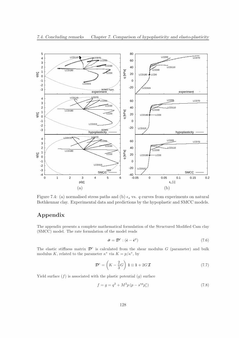
7.4. Concluding remarks Chapter 7. Comparison of hypoplasticity and elasto-plasticity
-4
-3
-2
-1
0
1
2
3
4
0 1 2 3 4 5 6
q/p e*
p/pe*
SBS
LCD0
LCD30
LCD55
LCD70LCD110
LCD180
LCD315
SMCC
-3
-2
-1
0
1
2
3
4
q/p e*
SOMS
LCD0
LCD30
LCD55
LCD70LCD110
LCD180
LCD315
hypoplasticity
-3
-2
-1
0
1
2
3
4
5
q/p e*
SOMS hypo.
LCD0
LCD30
LCD55LCD70LCD110
LCD180
LCD315
experiment
(a)
-40
-20
0
20
40
60
-0.05 0 0.05 0.1 0.15 0.2
q [k
Pa]
εs [-]
LCD0
LCD30
LCD55LCD70
LCD110
LCD180
LCD315
SMCC
-20
0
20
40
60
q [k
Pa]
LCD0
LCD30
LCD55 LCD70
LCD110
LCD180
LCD315
hypoplasticity
-20
0
20
40
60
80
q [k
Pa]
LCD0
LCD30
LCD55 LCD70
LCD110
LCD180
LCD315
experiment
(b)
Figure 7.4: (a) normalised stress paths and (b) ǫs vs. q curves from experiments on naturalBothkennar clay. Experimental data and predictions by the hypoplastic and SMCC models.
Appendix
The appendix presents a complete mathematical formulation of the Structured Modified Cam clay(SMCC) model. The rate formulation of the model reads
σ = De : (ǫ − ǫp) (7.6)
The elastic stiffness matrix De is calculated from the shear modulus G (parameter) and bulk
modulus K, related to the parameter κ∗ via K = p/κ∗, by
De =
(
K − 2
3G
)
1⊗ 1 + 2GI (7.7)
Yield surface (f) is associated with the plastic potential (g) surface
f = g = q2 +M2p (p− sepp∗c) (7.8)
128
7.4. Concluding remarks Chapter 7. Comparison of hypoplasticity and elasto-plasticity
M is the model parameter, sep (sensitivity) is the state variable and the quantity p∗c is related tothe state variable e (void ratio) through the equation
p∗c = pr exp
(
N − κ∗ ln (p/pr) − ln (1 + e)
λ∗ − κ∗
)
(7.9)
where pr is the reference stress 1 kPa and N and λ∗ are model parameters. Inside the yield surface(f < 0), ǫp = 0. For stress states on the yield surface, the plastic strain rate is given by:
ǫp =〈m : D
e : ǫ〉H + m : D
e : mm (7.10)
where the operator 〈x〉 := (x + |x|)/2 denotes the positive part of any scalar function x, H is theplastic modulus calculated from the consistency condition
H =M2pp∗cλ∗ − κ∗
[
sep tr(m) − k(
sep − sepf
)
√
tr2(m) +
(
A
1 −A
)
2
3dev(m) : dev(m)
]
(7.11)
and the tensor m is calculated by:
m =∂f
∂σ=M2(2p− sepp∗c)
31 + 3 dev(σ) (7.12)
sepf and k are model parameters. Evolution of state variables is governed by equations:
e = − (1 + e) ǫv sep = − k
λ∗ − κ∗(sep − sep
f )
√
(ǫpv)2
+A
1 −A(ǫps)
2(7.13)
ǫpv and ǫps are rates of plastic volumetric and shear strains respectively and A is model parameter.
129

Chapter 8
Summary and conclusions
The thesis traces the research into the constitutive modelling of fine-grained soils usingtheory of hypoplasticity. The developed constitutive model is from the practical point ofview equivalent to the Modified Cam clay model, since it requires the same number ofmaterial parameters with an equivalent physical meaning. However, due to the non-linearcharacter of the hypoplastic formulation, the quality of predictions by the proposed modelis at least comparable to more complex advanced elasto-plastic models.
From the mathematical standpoint, the model is positively homogeneous of degree 1 inD and for a given value of fd in T. Therefore, the behaviour of the fine-grained soil isassumed to be rate-independent. This is clearly a strong assumption that limits the validityof the material parameters only to certain range of loading rates. Positive homogeneityof degree 1 in T for given fd implies parallel normal compression lines of the slope λ∗ inthe ln(1 + e) vs. ln p space. Also, the behaviour is for a given degree of overconsolidationassumed to be scalable by the mean stress, which is according to experimental evidence areasonable approximation of the behaviour of clays.
The model requires four other material parameters in addition to λ∗. N determines theposition of the isotropic normal compression line, κ∗ the slope of the isotropic unloadingline in the ln(1 + e) vs. ln p space. Unlike in the Cam clay-type models, the slope ofthe unloading branch is exactly equal to the parameter κ∗ only for unloading from theisotropic normally consolidated state, at overconsolidated states the slope is higher, dueto the non-linear character of the model formulation. The next parameter, ϕc, defines thecritical state friction angle at triaxial compression and extension. The model makes use ofthe Matsuoka-Nakai shape of the critical state locus in the stress space, so for other Lodeangles the critical state friction angle is slightly higher than ϕc. This is well in agreementwith experimental data. The last parameter, r, controls the shear stiffness, which decreaseswith increasing r. This parameter is usually calibrated by means of a parametric study.
A shortcoming of hypoplastic models in general is an inevitable ”rachetting”, i.e. theextensive accumulation of strains during cyclic loading caused by the too soft response uponsharp reversals of the stress/strain paths directions. Niemunis and Herle [108] proposed
130

Chapter 8. Summary and conclusions
a modification of the hypoplastic equation by introducing so-called intergranular strainconcept that eliminates this shortcoming. The proposed model has been designed to beused with the intergranular strain enhancement by letting the tensor L to have the formappropriate to predict both the behaviour in the small strain range and upon sharp pathreversal (in this case the nonlinear part N‖D‖ of the hypoplastic equation is ruled out)and for continuing deformation (in limit the model response tends to the basic hypoplasticformulation).
It has been shown that the proposed form of the constitutive tensors L and N and thebarotropy and pyknotropy factors fd and fs allow us to derive a closed-form solution forswept-out-memory states, which compose a hypersurface in the stress – void ratio spacecalled swept-out-memory surface1. This surface is a close approximation of the state bound-ary surface, defined as boundary of all possible states in the stress – void ratio space. Pre-diction of the state boundary surface is an important property of the proposed model thatmakes it possible not only to compare the model response with relevant experimental data,but mainly it opens the way for further extensions of the model. The study in Chapter 3revealed an important shortcoming of the model – the swept-out-memory surface does nothave a reasonable shape for too high values of the ratio κ∗/λ∗. However, if κ∗/λ∗ is smallerthan approx. 1/4, the shape of the state boundary surface compares well with the shapeobserved experimentally.
Predictions by the proposed model were compared with a number of existing elasto-plasticand hypoplastic models, namely Modified Cam clay model, three surface kinematic hard-ening (3-SKH) model and a Grenoble-type hypoplastic model (CLoE). With regard to thedirectional response, the proposed model, together with the 3-SKH model, performed best.As expected, a simple Modified Cam clay model has shown a poor performance for loadingpaths directed inside the elastic region, while the non-linear character of the hypoplasticmodel led to at least qualitatively correct predictions for all loading directions. Predictionsof stress probes that followed after sharp stress-path reversal were further improved byapplying the intergranular strain concept. The 3-SKH model performed similarly to theproposed hypoplastic model. This is a consequence of the fact that although both modelsare developed using different mathematical concepts, they are both based on the similarphysical interpretation of the behaviour of fine-grained soils.
A study of the validity of a single set of material parameters for prediction of behaviour ofsoils at different overconsolidation ratios (OCR) revealed that if the proposed hypoplasticmodel is calibrated at higher OCR, it performs well for a broad range of OCRs, bothqualitatively and quantitatively. The Modified Cam clay model and the 3-SKH modelperformed in this case worst than the proposed hypoplastic model.
The last part of the thesis demonstrated a possibility for further extension of the model. Inparticular, the basic model was modified to predict the behaviour of clays with meta-stablestructure. The framework for the mechanical behaviour of natural clays by Cotecchia andChandler [34], according to which it is possible to relate the behaviour of natural and
1This closed-form solution is not available for other hypoplastic models, such as the model by vonWolffersdorff [141]
131

Chapter 8. Summary and conclusions
reconstituted clay through the state variable sensitivity, was applied. The sensitivity wasincorporated in such a way that the size of the state boundary surface was increased,other material properties were however kept unchanged. A suitable evolution equation forsensitivity then enabled us to predict the behaviour of clays with meta-stable structure.Predictions of the enhanced hypoplastic model were compared with predictions by itselasto-plastic ’equivalent’, structured Modified Cam clay model, developed in Chapter 7.It was again clearly demonstrated that with the same number of parameters of equivalentphysical interpretation the non-linear hypoplastic model leads to better predictions.
132
Chapter 9
Outlook
The proposed model is conceptually very simple, and the small number of material pa-rameters obviously does not allow us to tune the model predictions into great detail. Anyfurther modification of the model would, however, require extensive evaluation that wouldpinpoint systematic differences between model predictions and experiment. In this respectan independent evaluation by different researchers working in the field of constitutive mod-elling is particularly valuable.
Weifner [143] compared predictions by the proposed model with different hypoplastic mod-els for fine-grained soils [105, 54, 61], based on experimental data on Weald clay byHenkel [59, 60]. The data consist of isotropic loading and unloading tests and drainedand undrained triaxial tests starting from isotropic normally consolidated and overcon-solidated (OCR = 24) states. Weifner observed shortcoming of the model discussed inChapter 3 – the model does not perform realistically for too high values of the ratio κ∗/λ∗.If κ∗ was changed to sufficiently low value the model performed reasonably at normallyconsolidated states, but the response at isotropic unloading was too stiff. Because theinitial state of shear experiments was found by simulating the consolidation stress history,too stiff response in isotropic unloading led to apparently higher overconsolidation andtherefore the peak stiffness and dilatancy in tests at OCR = 24 was exaggerated.
Huang et al. [63] point out a different shortcoming of the proposed model – the model doesnot perform correctly under undrained conditions at normally consolidated states. Thisis an inevitable consequence of a hypoplastic formulation, which is characterised by thetranslated elliptical response envelope. In order to calibrate the model parameters λ∗ andκ∗ at isotropic loading and unloading conditions, the response envelope must be shifted insuch a way that under constant volume conditions an excessive decrease of the mean stressis predicted. Huang et al. proposed an approach to overcome this shortcoming. Startingfrom the hypoplastic formulation by Gudehus [53], they produced a hybrid elasto-plastic-hypoplastic model. At isotropic stress states the non-linear part vanishes, the model isincrementally bi-linear, i.e. equivalent to an elasto-plastic model. The predicted initial partof the undrained stress paths is then perpendicular to the p-axis. With higher deviatoricstresses the non-linear part is activated and hybrid elasto-plastic-hypoplastic predictions
133
Chapter 9. Outlook
are obtained. The formulation by Gudehus [53] is modified in such a way that the modelrequires parameters equivalent to the model from Chapter 2. The model by Huang et al.does not include pyknotropy, i.e. it can be only used for normally consolidated states anddoes not predict a unique critical state line in the stress vs. void ratio space. The model isnot positively homogeneous of degree 1 in T, so normal compression lines that correspondto higher ratio η = q/p do not have a slope of λ∗. However, the directional homogeneitywith respect to T (defined by Niemunis [106]) is satisfied so the model predicts asymptoticstates (in the stress space).
A conceptually similar approach to that by Huang et al. [63] to improve response ofhypoplastic models to undrained shearing, which is directly applicable to the model fromChapter 2, has been proposed by Niemunis [106]. In this case the linear part L of the modelis kept unchanged, at isotropic state the term ~m‖D‖ is replaced by ~r|~r : D|, where the unittensor ~r is (for any stress state) parallel to T. For ~D = ±~r we have |~r : D| = ‖D‖ and since~r = ~m the original hypoplastic response is recovered. For D ⊥ ~r, however, |~r : D| = 0 andresponse is hypoelastic and is controlled by the linear term L : D only. The hypoelasticresponse envelope is therefore squeezed in the direction of loading and elongated in thedirection of unloading, its shape is equivalent to that proposed by Huang et al. [63] andthe model also predicts initial portion of the undrained stress path perpendicular to thep-axis. For anisotropic stress states Niemunis [106] suggests interpolation between ~m‖D‖and ~r|~r : D| such that at the critical state surface (in the stress space) the response ispurely hypoplastic.
The next step in the evaluation of predictive capabilities of the model is the comparisonof its predictions with measurements on the boundary-value problem scale. The proposedmodel has been implemented into finite element code via a user-defined subroutine umat.fby Tamagnini [129] (direct perturbation method) and Arnold [4] (Fellin and Ostermannalgorithm [44]), both with and without intergranular strain concept. Masın and Herle[94] presented finite element simulations of the Heathrow Express trial tunnel [41] by theproposed model, Mohr-Coulomb model and a Modified Cam clay model. Although theproposed model predicts wider settlement trough than measured in the field, its predictionsare significantly more realistic than predictions by the simpler models. Further evaluationof the model with respect to boundary-value problems is needed.
The behaviour of fine-grained soils is markedly rate-dependent, and the assumption of rate-independence is reasonable only for a relatively narrow ranges of loading rates. This factnecessarily complicates any experimental program as in looking for parameters relevant tothe given boundary value problem the soil should be tested at the loading rates similarto the field. These rates can only be estimated, often very roughly. Rate effects could berelatively easily incorporated into the proposed model by adopting an approach proposed byNiemunis [106] and further discussed by Gudehus [54]. The stretching rate D is decomposedinto the viscous (Dv) and non-viscous (D − Dv) part. The viscous part Dv has the sametensorial direction as the non-linear part of the reference model ( ~m), its magnitude isdependent on overconsolidation ratio via two new material parameters. The referencestress pr is dependent on the stretching rate ‖D‖. It has been shown [106, 54] that ahypoplastic model modified in this way can qualitatively correctly predict creep, relaxation
134
Chapter 9. Outlook
and response to strain rate jumps. A thorough evaluation of this concept when used withthe proposed model would, however, be needed.
During the geological history natural soils undergo compression underK0 conditions, whichoften leads to one-dimensionally oriented fabric. This fabric implies a textural anisotropy,which may be observed even when the soil is tested from isotropic stress state. The modelof Chapter 2 is orthotropic with the planes of symmetry given by eigenvectors of T, atisotropic stress state, however, the response is isotropic [107]. Incorporation of anisotropyinto hypoplasticity has been first proposed by Wu [150, 152]. He replaced the non-linearpart N of his early version of hypoplastic model [151] by Aa : N, where Aa is a fourth-ordertransversally isotropic tensor. As discussed by Niemunis [107], shortcoming of this rathersimple approach is that the modification of the non-linear part N only does not provide thedesirable independent control over dilatancy, strength and stiffness, as in hypoplasticitythese features are implied by a combined effect of L and N. Niemunis [107] thereforesuggested a different modification, which is applied to the formulation from Eq. (2.8)and keeps the critical state locus (incorporated via Y ) and a hypoplastic flow rule (~m)unchanged. Modification of the linear term L and a pyknotropy factor fd only enabledhim to improve the dilatancy curve and the shape of the undrained stress path producedby the model. Further development would be needed to incorporate most effects of texturalanisotropy, such as anisotropic shape of the state boundary surface, stiffness, dilatancy andshape of the undrained stress path.
With regard to the model for structured soils (Chapter 6), more research would be requiredto incorporate true cohesion caused by interparticle bonding. A simple idea of the replace-ment of stress tensor T by a transformed stress tensor Tt according to equation (6.7) hasundesired effects. Namely, the normal compression lines are shifted in the ln(1+ e) vs. ln pspace, they are in this space no-more linear and undefined for p→ 0, so the parameter λ∗
loses its physical meaning. Also other material properties (e.g. shear and bulk stiffnesses),which are measured with respect to the true stress T, now relate to the transformed stressTt. The model loses its positive homogeneity of degree one in T so it does not predict anylonger asymptotic (swept-out-memory) states in the true stress space T.
The model for structured clays of Chapter 6 can be straightforwardly applied to doubleporosity materials. A typical example of these materials are double-porosity clayfills fromopen-cast coal mines in north Bohemia, which consist of clay lumps up to half meter in size,dumped without any compaction. In addition to the intragranular porosity (porosity ofclay lumps) the overall void ratio is increased by the intergranular porosity (voids betweenclay lumps). Mechanical behaviour of such a composite material is relatively complex. Aframework for its description has been put forward by Masın et al. [93], a similar approachhas been suggested by Koliji et al. [74]. The reference constitutive model now describesthe behaviour of the material of clay lumps, whereas sensitivity s is a measure of addi-tional structure caused by intergranular porosity. The evolution of sensitivity representsdegradation of the intergranular porosity, i.e. closing the voids between individual claylumps. The evolution equation for sensitivity may be calibrated by means of compressionexperiments on the material of clay lumps and corresponding granulated material. Due tothe dimensions of experimental apparatuses the material with reduced granulometry must
135

Chapter 9. Outlook
often be used.
As the last point, a modification of the proposed model to predict the behaviour of un-saturated soils will be discussed. An attempt to incorporate partial saturation into anexisting hypoplastic equation has been proposed by Gudehus [52]. In his work the effec-tive stress principle is applied, i.e. the existing hypoplastic equation is without furthermodification written in terms of the effective stress in partially saturated soils, startingwith the definition by Bishop [15] and continuing with a more complex one. Qualitativelycorrect predictions for some loading paths are claimed. The model was, primarily from themathematical point of view, further investigated by Niemunis [106]. However, as discussedby Wheeler and Karube [144], the model does not enable us to represent some of the mostfundamental features of unsaturated soil behaviour, most notably the correct pattern ofswelling and collapse on wetting. To overcome this problem, a scalar state variable thatrepresents normal forces on grain contacts produced by the menisci of the pore fluid isneeded, in addition to the tensorial stress variable that represents the action of externalforces. An extensive research in unsaturated soil behaviour did not lead to a unique choiceof the two state variables that would be ideal. In general, simple state variables (used,e.g., by Alonso et al. [3]) lead to more complex constitutive models. More complex statevariables (advocated, e.g., by Loret and Khalili [83]) simplify the definition of the consti-tutive models, but complicate description of the stress state in such a way that it may bedifficult to devise simple experimental tests to measure relevant soil parameters.
An attempt to develop a hypoplastic model for granular materials considering a scalarstate variable that represents the action of capillary mensici has been presented by Baueret al. [11]. Their model is, however, oversimplified – the only modification of the originalequation is that the granulate hardness hs (an equivalent of a reference pressure pr ofthe model of Chapter 2) is made dependent on degree of saturation. In this way differentcompressibilities of soils with different moisture contents are predicted. However, the modeldoes not predict the behaviour of soils when subjected to changes in degree of saturation.
A more comprehensive modification of the model of Chapter 2 is being developed byMasın [91]. The approach by Alonso et al. [3] is used, the stress state is characterisedby net stress σ = σt − 1ua and suction s = ua − uw, where σt is total stress, ua anduw are the pressures of the pore air and water respectively. The influence of suction istreated similarly to the model by Alonso et al. [3]. Equivalent suction s∗e is introducedas the additional state variable that characterises the previous suction-loading history, thestraining due to suction changes at overconsolidated states is controlled by the non-linearhypoplastic equation resembling the basic form of hypoplastic models for saturated soils.A consistency condition for the swept-out-memory surface from Chapter 3 is introduced inorder to model wetting induced collapse. The model therefore shares some features withthe bounding surface plasticity models [38].
The next step in the development of the hypoplastic model for unsaturated soils will be theapplication of more complex state variables (such as those discussed by Khalili et al. [72])and a comparison of the merits and disadvantages of both formulations. Subsequently, thehysteretic soil-water characteristic curve should be incorporated.
136

References
[1] A. Al Tabbaa and D. M. Wood. An experimentally based ”bubble” model for clay.In Proc. 3th Int. Conf. on Numerical Models in Geomechanics. Niagara Falls, 1989.
[2] M. A. Allman and J. H. Atkinson. Mechanical properties of reconstituted Bothkennarsoil. Geotechnique, 42(2):289–301, 1992.
[3] E. Alonso, A. Gens, and A. Josa. A constitutive model for partially saturated soils.Geotechnique, 40(3):405–430, 1990.
[4] M. Arnold. Private communication. University of Dresden, 2006.
[5] A. Asaoka. Compaction of sand and consolidation of clay: a super/subloading yieldsurface approach. In Proc. 11th Int. Conference IACMAG, volume 4, pages 121–140.Turin, Italy, 2005.
[6] J. H. Atkinson, D. Richardson, and S. E. Stallebrass. Effects of recent stress historyon the stiffness of over–consolidated soil. Geotechnique, 40(4):531–540, 1990.
[7] B. A. Baudet. Modelling effects of structure in soft natural clays. PhD thesis, CityUniversity, London, 2001.
[8] B. A. Baudet and S. E. Stallebrass. A constitutive model for structured clays.Geotechnique, 54(4):269–278, 2004.
[9] E. Bauer. Modelling of critical stress in hypoplasticity. In NUMOG V, pages 15–20,Davos, 1995. Balkema.
[10] E. Bauer. Calibration of a comprehensive constitutive equation for granular materials.Soils and Foundations, 36(1):13–26, 1996.
[11] E. Bauer, W. Cen, Y. Zhu, K. Kast, and S. F. Tantono. Modelling of partly saturatedweathered broken rock. In H. F. Schweiger, editor, Proc. 6th European Conferenceon Numerical Methods in Geomechanics (NUMGE06), Graz, Austria, pages 87–92.Taylor & Francis Group, London, 2006.
[12] E. Bauer and W. Wu. A hypoplastic model for granular soils under cyclic loading.In D. Kolymbas, editor, Modern Approaches to Plasticity, pages 247–258. ElsevierScience Publishers B.V., 1993.
137

REFERENCES REFERENCES
[13] E. Bauer and W. Wu. Extension of hypoplastic constitutive model with respectto cohesive powders. In Siriwardane and Zeman, editors, Computer methods andadvances in geomechnics, pages 531–536. A.A.Balkema, Rotterdam, 1994.
[14] A. Beghini and P. Bazant. Discussion of paper ”Shear and objective stress ratesin hypoplasticity”. International Journal for Numerical and Analytical Methods inGeomechanics, 28:365–372, 2004.
[15] A. W. Bishop. The principle of effective stress. Teknisk Ukeblad, 106(39):859–863,1959.
[16] R. I. Borja, C.-H. Lin, and F. J. Montans. Cam–clay plasticity, Part IV: Implicitintegration of anisotropic bounding surface model with nonlinear hyperelasticity andellipsoidal loading function. Comp. Meth. Appl. Mech. Engng., 190:3293–3323, 2001.
[17] J. B. Burland. On the compressibility and shear strength of natural clays.Geotechnique, 40(3):329–378, 1990.
[18] R. Butterfield. A natural compression law for soils. Geotechnique, 29(4):469–480,1979.
[19] L. Callisto. Studio sperimentale su un’argilla naturale: il comportamento meccanicodell’argilla di Pisa. PhD thesis, Universita La Sapienza, Roma, 1996.
[20] L. Callisto and G. Calabresi. Mechanical behaviour of a natural soft clay.Geotechnique, 48(4):495–513, 1998.
[21] L. Callisto, A. Gajo, and D. Muir Wood. Simulation of true triaxial tests on naturaland reconstituted pisa clay. Geotechnique, 52(9):649–666, 2002.
[22] L. Callisto and S. Rampello. Shear strength and small–strain stiffness of a naturalclay under general stress conditions. Geotechnique, 52(8):547–560, 2002.
[23] L. Callisto and S. Rampello. An interpretation of structural degradation for threenatural clays. Canadian Geotechnical Journal, 41:392–407, 2004.
[24] F. Calvetti, C. Tamagnini, and G. Viggiani. On the incremental behaviour of granularsoils. In NUMOG VIII, pages 3–9. Swets & Zeitlinger, 2002.
[25] M. Cecconi, A. DeSimone, C. Tamagnini, and G. M. B. Viggiani. A constitutivemodel for granular materials with grain crushing and its application to a pyroclasticsoil. International Journal for Numerical and Analytical Methods in Geomechanics,26:1531–1560, 2002.
[26] R. Chambon. Une classe de lois de comportement incrementalement nonlinaires pourles sols non visqueux, resolution de quelques problemes de coherence. C. R. Acad.Sci., 308(II):1571–1576, 1989.
138

REFERENCES REFERENCES
[27] R. Chambon. Discussion of paper “shear and objective stress rates in hypoplasticity”by d. kolymbas and i. herle. International Journal for Numerical and AnalyticalMethods in Geomechanics, 28:365–372, 2004.
[28] R. Chambon and J. Desrues. Bifurcation par localisation et non lineariteincrementale: un example heuristique d’analyse complete. In Plastic Instability,pages 101–113, Paris, France, 1985. Presses ENPC.
[29] R. Chambon, J. Desrues, W. Hammad, and R. Charlier. CLoE, a new rate–type con-stitutive model for geomaterials. theoretical basis and implementation. InternationalJournal for Numerical and Analytical Methods in Geomechanics, 18:253–278, 1994.
[30] C. R. I. Clayton and G. Heymann. Stiffness of geomaterials at very small strains.Geotechnique, 51(3):245–255, 2001.
[31] D. Costanzo, G. Viggiani, and C. Tamagnini. Directional response of a reconsti-tuted fine grained soil. Part I: Experimental investigation. International Journal forNumerical and Analytical Methods in Geomechanics, 30(13):1283–1301, 2006.
[32] F. Cotecchia. The effects of structure on the properties of an Italian Pleistocene clay.PhD thesis, University of London, 1996.
[33] F. Cotecchia and J. Chandler. The influence of structure on the pre–failure behaviourof a natural clay. Geotechnique, 47(3):523–544, 1997.
[34] F. Cotecchia and J. Chandler. A general framework for the mechanical behaviour ofclays. Geotechnique, 50(4):431–447, 2000.
[35] T. Cuccovillo and M. R. Coop. The measurement of local axial strains in tiaxial testsusing LVDT’s. Geotechnique, 47(1):167–171, 1997.
[36] R. Cudmani and V. A. Osinov. The cavity expansion problem for the interpretationof cone penetration and pressuremeter tests. Canadian Geotechnical Journal, 38:622–638, 2001.
[37] M. Cudny and P. A. Vermeer. On the modelling of anisotropy and destruction of softclays within the multi-laminate framework. Computers and Geotechnics, 31(1):1–22,2004.
[38] Y. F. Daffalias. Bounding surface plasticity. I: Mathematical foundation and hy-poplasticity. Journal of Engineering Mechanics ASCE, 112(9):966–987, 1986.
[39] F. Darve. The expression of rheological laws in incremental form and the main classesof constitutive equations. In F. Darve, editor, Geomaterials: Constitutive Equationsand Modelling, pages 123–148. Elsevier, 1990.
[40] R. de Borst and O. Heeres. A unified approach to the implicit integration of standard,non-standard and viscous plasticity models. International Journal for Numerical andAnalytical Methods in Geomechanics, 26:1059–1070, 2002.
139

REFERENCES REFERENCES
[41] A. P. Deane and R. H. Basset. The heathrow express trial tunnel. Proc. Instn. CivilEngineers, 113:144–156, 1995.
[42] J. Desrues. Private communication. Grenoble, 2004.
[43] J. Desrues and R. Chambon. Shear band analysis for granular materials: the questionof incremental non–linearity. Ingenieur–Archiv, 59:187–196, 1989.
[44] W. Fellin and A. Ostermann. Consistent tangent operators for constitutive rate equa-tions. International Journal for Numerical and Analytical Methods in Geomechanics,26:1213–1233, 2002.
[45] R. J. Finno, I. S. Harahap, and P. J. Sabatini. Analysis of braced excavations withcoupled finite element formulations. Computers and Geotechnics, 12:91–114, 1989.
[46] A. Gajo and D. Muir Wood. A new approach to anisotropic, bounding surfaceplasticity: general formulation and simulations of natural and reconstituted claybehaviour. International Journal for Numerical and Analytical Methods in Geome-chanics, 25:207–241, 2001.
[47] J. Graham and G. T. Houlsby. Anisotropic elasticity of a natural clay. Geotechnique,33(2):165–180, 1983.
[48] J. Graham, M. L. Noonan, and K. V. Lew. Yield stress and strain relationship in anatural plastic clay. Canadian Geotechnical Journal, 20:502–516, 1983.
[49] R. J. Grant, S. E. Stallebrass, and R. N. Taylor. Prediction of pre-failure groundmovements: Physical and numerical techniques. In Proc. 14th Int. Conf. Soil Me-chanics and Foundation Engineering, pages 663–668. Balkema Rotterdam, 1996.
[50] G. Gudehus. A comparison of some constitutive laws for soils under radially sym-metric loading and unloading. In Proc. 3rd Int. Conf. on Numerical Methods inGeomechanics, pages 1309–1323. Aachen, 1979.
[51] G. Gudehus. Attractors for granular storage and flow. In 3rd European Symposium– Storage and Flow of Particulate Solids, Paper for the conf. ’Partec 95’, pages 333–345, 1995.
[52] G. Gudehus. A comprehensive concept for non-saturated granular bodies. In Alonsoand Delage, editors, 1st Int. Conference on Unsaturated Soils, Paris, France, vol-ume 2, pages 725–737. Balkema, Rotterdam, 1995.
[53] G. Gudehus. A comprehensive constitutive equation for granular materials. Soilsand Foundations, 36(1):1–12, 1996.
[54] G. Gudehus. A visco-hypoplastic constitutive relation for soft soils. Soils and Foun-dations, 44(4):11–25, 2004.
140
REFERENCES REFERENCES
[55] G. Gudehus, M. Goldscheider, and H. Winter. Mechanical properties of sand and clayand numerical intergration methods: some sources of errors and bounds of accuracy.In G. Gudehus, editor, Finite Elements in Geomechanics, pages 121–150. Wiley,1977.
[56] V. Hajek and D. Masın. An evaluation of constitutive models to predict the be-haviour of fine-grained soils with different degrees of overconsolidation. In H. F.Schweiger, editor, Proc. 6th European Conference on Numerical Methods in Geome-chanics (NUMGE06), Graz, Austria, pages 49–55. Taylor & Francis Group, London,2006.
[57] K. Hashiguchi. Two– and three–surface models of plasticity. In V Int. Conf. Num.Meth. in Geomechanics, pages 285–292, Nagoya, Japan, 1985. Balkema, Rotterdam.
[58] M. Hattab and P.-Y. Hicher. Dilating behaviour of overconsolidated clay. Soils andFoundations, 44(4):27–40, 2004.
[59] D. J. Henkel. The effect of overconsolidation on the behaviour of clays during shear.Geotechnique, 6:139–150, 1956.
[60] D. J. Henkel and V. A. Sowa. The influence of stress history on stress paths inundrained triaxial tests on clay. Laboratory Shear Testing of Soils, ASTM SpecialTechnical Publication, 361:280–291, 1963.
[61] I. Herle and D. Kolymbas. Hypoplasticity for soils with low friction angles. Computersand Geotechnics, 31(5):365–373, 2004.
[62] D. W. Hight, A. J. Bond, and J. D. Legge. Characterisation of the Bothkennar clay:an overview. Geotechnique, 42(2):199–217, 1992.
[63] W.-X. Huang, W. Wu, D.-A. Sun, and S. Sloan. A simple hypoplastic model fornormally compressed clay. Acta Geotechnica, 1(1):15–27, 2006.
[64] M. Hvorslev. Physical components of the shear strength of saturated clays. In ShearStrength of Cohesive Soils, proc. ASCE Research Conf. Boulder, Colorado, 1960.
[65] P. J. Ingram. The applicaton of numerical models to natural stiff clays. PhD thesis,City University, London, 2000.
[66] J. Jaky. The coefficient of earth pressure at rest. Journal for Society of HungarianArchitects and Engineers, pages 355–357, 1944.
[67] R. J. Jardine, M. J. Symes, and J. B. Burland. The measurement of soil stiffness inthe triaxial apparatus. Geotechnique, 34(3):323–340, 1984.
[68] V. Jovicic. The measurement and interpretation of small strain stiffness of soil. PhDthesis, City University, London, 1997.
141

REFERENCES REFERENCES
[69] V. Jovicic and M. R. Coop. The measurement of stiffness anisotropy in clays withbender element tests in the triaxial apparatus. Geotechnical Testing Journal, 21(1):3–10, 1998.
[70] C. Karcher. Tagebaubedingte Deformationen im Lockergestein. Veroffentlichungendes Institutes fur Bodenmechanik und Felsmechanik der Universitat Fridericiana inKarlsruhe, 2003. Heft 160.
[71] M. Kavvadas and A. Amorosi. A constitutive models for structured soils.Geotechnique, 50(3):263–273, 2000.
[72] N. Khalili, F. Geiser, and G. E. Blight. Effective stress in unsaturated soils: reviewwith new evidence. International Journal of Geomechanics, 4(2):115–126, 2004.
[73] M. M. Kirkgard and P. V. Lade. Anisotropic three–dimmensional behaviour of anormally consolidated clay. Canadian Geotechnical Journal, 30:848–858, 1993.
[74] A. Koliji, L. Vulliet, L. Laloui, A. Carminati, A. Kaestner, H. Fluhler, P. Lehmann,R. Hassanein, E. Lehmann, and P. Vontobel. Structure degradation of dry aggregatedsoil: experimental evidence and model formulation. In A. Miller, C. E. Zapata, S. L.Houston, and D. G. Fredlund, editors, 4th Int. Conference on Unsaturated Soils,Carefree, Arizona, volume 2, pages 2174–2185. ASCE, USA, 2006.
[75] D. Kolymbas. Eine konstitutive Theorie fur Boden und andere kornige Stoffe. PhDthesis, Karlsruhe University, Germany, 1978.
[76] D. Kolymbas. Computer-aided design of constitutive laws. International Journal forNumerical and Analytical Methods in Geomechanics, 15:593–604, 1991.
[77] D. Kolymbas. An outline of hypoplasticity. Archive of Applied Mechanics, 61:143–151, 1991.
[78] D. Kolymbas and I. Herle. Shear and objective stress rates in hypoplasticity. Interna-tional Journal for Numerical and Analytical Methods in Geomechanics, 27:733–744,2003.
[79] R. Lagioia and R. Nova. An experimental and theoretical study of the behaviour ofa calcarenite in triaxial compression. Geotechnique, 45(4):633–648, 1995.
[80] J. Lanier, D. Caillerie, R. Chambon, G. Viggiani, P. Besuelle, and J. Desrues. Ageneral formulation of hypoplasticity. International Journal for Numerical and An-alytical Methods in Geomechanics, 28:1461–1478, 2004.
[81] P. I. Lewin and J. B. Burland. Stress-probe experiments on saturated normallyconsolidated clay. Geotechnique, 20(1):38–56, 1970.
[82] M. D. Liu and J. P. Carter. A structured Cam Clay model. Canadian GeotechnicalJournal, 39:1313–1332, 2002.
142
REFERENCES REFERENCES
[83] B. Loret and N. Khalili. An effective stress elastic-plastic model for unsaturatedporous media. Mechanics of Materials, 34:97–116, 2002.
[84] L. X. Luccioni, J. M. Pestana, and R. L. Taylor. Finite element implementation ofnon-linear elastoplastic constitutive laws using local and global explicit algorithmswith automatic error control. International Journal for Numerical Methods in Engi-neering, 50:1191–1212, 2001.
[85] H. Matsuoka and T. Nakai. Stress–deformation and strength characteristics of soilunder three different principal stresses. In Proc. Japanese Soc. of Civil Engineers,volume 232, pages 59–70, 1974.
[86] D. Masın. Laboratory and Numerical Modelling of Natural Clays. MPhil Thesis, CityUniversity, London, 2004.
[87] D. Masın. A hypoplastic constitutive model for clays. International Journal forNumerical and Analytical Methods in Geomechanics, 29(4):311–336, 2005.
[88] D. Masın. A hypoplastic constitutive model for clays with meta-stable structure.Canadian Geotechnical Journal (accepted), 2006.
[89] D. Masın. Incorporation of meta-stable structure into hypoplasticity. In Proc. Int.Conference on Numerical Simulation of Construction Processes in Geotechnical En-gineering for Urban Environment, pages 283–290. Bochum, Germany, 2006.
[90] D. Masın. Comparison of elasto-plastic and hypoplastic modelling of structuredclays. In Proc. International Workshop on Constitutive Modelling - Development,Implementation, Evaluation, and Application (in print). Hong Kong, China, 2007.
[91] D. Masın. A hypoplastic model for unsaturated soils based on barcelona basic model.In Proc. Tenth International Symposium on Numerical Models in Geomechanics (inpreparation). Rhodes, Greece, 2007.
[92] D. Masın, R. Chambon, and J. Desrues. CLoE model modified to predict the be-haviour of normally compressed clays. In Proc. 11th Int. Conference IACMAG, vol-ume 2, pages 417–424. Turin, Italy, 2005.
[93] D. Masın, V. Herbstova, and J. Bohac. Properties of double porosity clayfills andsuitable constitutive models. In Proc. 16th Int. Conference ICSMGE, volume 2, pages827–830. Osaka, Japan, 2005.
[94] D. Masın and I. Herle. The influence of a constitutive assumption on the predictionsof deformations around a tunnel in fine-grained soils (in czech). In In Proc. 33rd
Conf. Zakladanı Staveb. Brno, Czech Republic, 2005.
[95] D. Masın and I. Herle. Numerical analyses of a tunnel in london clay using differentconstitutive models. In In Proc. 5th Int. Symposium TC28 Geotechnical Aspects ofUnderground Construction in Soft Ground, pages 595–600. Amsterdam, The Nether-lands, 2005.
143

REFERENCES REFERENCES
[96] D. Masın and I. Herle. State boundary surface in hypoplasticity. In W. Wu and H. S.Yu, editors, Proc. Int. workshop Modern trends in geomechanics, Vienna, Austria,pages 117–128. Springer, Berlin, 2005.
[97] D. Masın and I. Herle. State boundary surface of a hypoplastic model for clays.Computers and Geotechnics, 32(6):400–410, 2005.
[98] D. Masın, S. E. Stallebrass, and J. H. Atkinson. Laboratory modelling of naturalstructured clays. In Wermeer, Schweiger, Karstunen, and Cudny, editors, In Proc.International Workshop on Geotechnics of Soft Soils – Theory and Practice, pages253–263. Noordwijkerhout, Netherlands, 2003.
[99] D. Masın, C. Tamagnini, G. Viggiani, and D. Costanzo. Directional response of areconstituted fine grained soil. Part II: performance of different constitutive mod-els. International Journal for Numerical and Analytical Methods in Geomechanics,30(13):1303–1336, 2006.
[100] P.-M. Mayer. Verformungen und Spannungsanderungen im Boden durch Schlitzwand-herstellung und Baugrubenaushub. Veroffentlichungen des Institutes fur Boden-mechanik und Felsmechanik der Universitat Fridericiana in Karlsruhe, 2000. Heft151.
[101] P. W. Mayne and F. H. Kulhawy. K0–OCR relationships in soil. In Proc. ASCE J.Geotech. Eng. Div., volume 108, pages 851–872, 1982.
[102] Z. Mroz, V. A. Norris, and O. C. Zienkiewicz. An anisotropic hardening model forsoils and its application to cyclic loading. International Journal for Numerical andAnalytical Methods in Geomechanics, 2:203–221, 1978.
[103] Z. Mroz, V. A. Norris, and O. C. Zienkiewicz. Application of an anisotropic hardeningmodel in the analysis of elasto-plastic deformation of soil. Geotechnique, 29(1):1–34,1979.
[104] D. Muir Wood. Soil behaviour and critical state soil mechanics. Cambridge UniversityPress, 1990.
[105] A. Niemunis. A visco-plastic model for clay and its FE implementation. In E. Dem-bicki, W. Cichy, and L. Balachowski, editors, Recent results in mechanics of soils androcks., pages 151–162. TU Gdansk, 1996.
[106] A. Niemunis. Extended hypoplastic models for soils. Habilitation thesis, Ruhr-University, Bochum, 2002.
[107] A. Niemunis. Anisotropic effects in hypoplasticity. In Di Benedetto et al., editor,Deformation Characteristics of Geomaterials, pages 1211–1217, 2003.
[108] A. Niemunis and I. Herle. Hypoplastic model for cohesionless soils with elastic strainrange. Mechanics of Cohesive-Frictional Materials, 2:279–299, 1997.
144

REFERENCES REFERENCES
[109] A. Niemunis and S. Krieg. Viscous behaviour of soil under oedometric conditions.Canadian Geotechnical Journal, 33:159–168, 1996.
[110] A. Niemunis, K. Nubel, and C. Karcher. The consistency conditions for density limitsof hypoplastic constitutive law. Task Quarterly, 4(3):412–420, 2000.
[111] R. Nova, R. Castellanza, and C. Tamagnini. A constitutive model for bonded geo-materials subject to mechanical and/or chemical degradation. International Journalfor Numerical and Analytical Methods in Geomechanics, 27:705–732, 2003.
[112] K. Nubel and R. Cudmani. Examples of finite element calculations with the hy-poplastic law. In D. Kolymbas, editor, Constitutive Modelling of Granular Materials,pages 523–538. Springer, 2000.
[113] J. H. Prevost. Mathematical modelling of monotonic and cyclic undrained clay be-haviour. International Journal for Numerical and Analytical Methods in Geomechan-ics, 1:195–216, 1977.
[114] S. Rampello and L. Callisto. A study on the subsoil of the tower of pisa based onresults from standard and high–quality samples. Canadian Geotechnical Journal,35(6):1074–1092, 1998.
[115] J. R. Rice. The localization of plastic deformations. In Koiter, editor, Theoreticaland Applied Mechanics, pages 207–220. North–Holland, 1976.
[116] G. Rocchi, M. Fontana, and M. Da Prat. Modelling of natural soft clay destructionprocesses using viscoplasticity theory. Geotechnique, 53(8):729–745, 2003.
[117] K. H. Roscoe and J. B. Burland. On the generalised stress-strain behaviour of wetclay. In J. Heyman and F. A. Leckie, editors, Engineering Plasticity, pages 535–609.Cambridge: Cambridge Univesrity Press, 1968.
[118] M. Rouainia and D. Muir Wood. A kinematic hardening constitutive model fornatural clays with loss of structure. Geotechnique, 50(2):153–164, 2000.
[119] M. Rouainia and D. Muir Wood. Implicit numerical integration for a kinematichardening soil plasticity model. International Journal for Numerical and AnalyticalMethods in Geomechanics, 25:1305–1325, 2001.
[120] P. Royis and T. Doanh. Theoretical analysis of strain response envelopes usingincrementally non-linear constitutive equations. International Journal for Numericaland Analytical Methods in Geomechanics, 22(2):97–132, 1998.
[121] J. W. Rudnicki and J. R. Rice. Conditions for the localization of deformation inpressure–sensitive dilatant materials. Journal of the Mechanics and Physics of Solids,23:371–394, 1975.
[122] A. N. Schofield and C. P. Wroth. Critical state soil mechanics. McGraw-Hill BookCo., London, 1968.
145

REFERENCES REFERENCES
[123] P. R. Smith, R. J. Jardine, and D. W. Hight. The yielding of Bothkennar clay.Geotechnique, 42(2):257–274, 1992.
[124] H. D. St. John, D. M. Potts, R. J. Jardine, and K. G. Higgins. Prediction andperformance of ground response due to construction of a deep basement at 60Victoria Embankment. In G. T. Houlsby and A. N. Schofield, editors, PredictiveSoil Mechanics (Wroth Mem. Symp.). Thomas Telford, London, 1993.
[125] S. E. Stallebrass. Modelling the efects of recent stress history on the behaviour ofoverconsolidated soils. PhD thesis, City University, London, 1990.
[126] S. E. Stallebrass, J. H. Atkinson, and D. Masın. Manufacture of samples of overcon-solidated clay by laboratory sedimentation. Geotechnique (accepted), 2007.
[127] S. E. Stallebrass and R. N. Taylor. Prediction of ground movements in overconsoli-dated clay. Geotechnique, 47(2):235–253, 1997.
[128] A. Takahashi, D. W. H. Fung, and R. J. Jardine. Swelling effects on mechanicalbehaviour of natural london clay. In Proc. 16th Int. Conference ICSMGE, volume 2,pages 443–446. Osaka, Japan, 2005.
[129] C. Tamagnini. Private communication. University of Perugia, 2006.
[130] C. Tamagnini, D. Masın, D. Costanzo, and G. Viggiani. An evaluation of differentconstitutive models to predict the directional response of a reconstituted fine-grainedsoils. In W. Wu and H. S. Yu, editors, Proc. Int. workshop Modern trends in geome-chanics, Vienna, Austria, pages 143–157. Springer, Berlin, 2005.
[131] C. Tamagnini, D. Masın, G. Viggiani, and D. Costanzo. An evaluation of differentconstitutive models to predict the directional response of a reconstituted fine-grainedsoils. In Proc. Int. workshop Modern trends in geomechanics (in print). Vienna,Austria, 2005.
[132] C. Tamagnini and G. Viggiani. On the incremental non-linearity of soils. Part I:theoretical aspects. Rivista Italiana di Geotecnica, 36(1):44–61, 2002.
[133] C. Tamagnini, G. Viggiani, and R. Chambon. A review of two different approaches tohypoplasticity. In D. Kolymbas, editor, Constitutive modelling of granular materials,pages 107–144. Springer, 2000, 2000.
[134] C. Tamagnini, G. Viggiani, R. Chambon, and J. Desrues. Evaluation of differentstrategies for the integration of hypoplastic constitutive equations: Application tothe CLoE model. Mechanics of Cohesive-Frictional Materials, 5:263–289, 2000.
[135] S. Teachavorasinskun and T. Amornwithayalax. Elastic shear modulus of bangkokclay during undrained triaxial compression. Geotechnique, 52(7):537–540, 2002.
[136] J. Tejchman and I. Herle. A ”class A” prediction of the bearing capacity of planestrain footings on sand. Soils and Foundations, 39(5):47–60, 1999.
146

REFERENCES REFERENCES
[137] C. A. Truesdell. Hypo–elastic shear. Journal of Applied Physics, 27:441–447, 1956.
[138] H. A. M. van Eekelen. Isotropic yield surface in three dimensions for use in soilmechanics. International Journal for Numerical and Analytical Methods in Geome-chanics, 4:89–101, 1980.
[139] G. Viggiani and J. H. Atkinson. Stiffness of fine–grained soil at very small strains.Geotechnique, 45(2):245–265, 1995.
[140] G. Viggiani and C. Tamagnini. Ground movements around excavations in granularsoils: a few remarks on the influence of the constitutive assumptions on FE predic-tions. Mechanics of Cohesive-Frictional Materials, 5(5):399–423, 2000.
[141] P. A. von Wolffersdorff. A hypoplastic relation for granular materials with a pre-defined limit state surface. Mechanics of Cohesive-Frictional Materials, 1:251–271,1996.
[142] C. C. Wang. A new representation theorem for isotropic tensor functions. Archivefor Rational Mechanics and Analysis, 36:166–223, 1970.
[143] T. Weifner. Review and extension of hypoplastic equations. PhD thesis, Universityof Innsbruck, Austria, 2005.
[144] S. Wheeler and D. Karube. State of the art report - constitutive modelling. In 1st
Int. Conference on Unsaturated Soils, Paris, France, volume 3, pages 1323–1356.Balkema, Rotterdam, 1995.
[145] S. J. Wheeler, A. Naatanen, M. Karstunen, and M. Lojander. An anisotropic elasto-plastic model for soft clays. Canadian Geotechnical Journal, 40:403–418, 2003.
[146] A. J. Whittle, Y. M. A. Hashash, and R. V. Whitman. Analysis of deep excavationin Boston. Journal of Geotechnical Engineering ASCE, 119(1):69–90, 1993.
[147] D. M. Wood. Some aspects of the Mechanical Behaviour of Kaolin under TrulyTriaxial Conditions of Stress and Strain. PhD thesis, University of Cambridge, 1974.
[148] C. Wroth and G. Houlsby. Soil mechanics - property characterisation, and analysisprocedures. In Proc. 11th Conf. Soil. Mech., San Francisco, volume 1, pages 1–55,1985.
[149] W. Wu. Hypoplastizitat als mathematisches Modell zum mechanischen Verhaltengranularer Stoffe. PhD thesis, Karlsruhe University, Germany, 1992.
[150] W. Wu. Rational approach to anisotropy of sand. International Journal for Numericaland Analytical Methods in Geomechanics, 22:921–940, 1998.
[151] W. Wu and E. Bauer. A simple hypoplastic constitutive model for sand. InternationalJournal for Numerical and Analytical Methods in Geomechanics, 18:833–862, 1994.
147

REFERENCES REFERENCES
[152] W. Wu and W. Huang. Rational approach to anisotropy of rocks. In Proc. EUROCKSymposium, pages 623–628. Aachen, Germany, 2000.
[153] W. Wu and D. Kolymbas. Hypoplasticity then and now. In D. Kolymbas, editor,Constitutive Modelling of Granular Materials. Springer, Berlin, 2000.
[154] W. Wu and A. Niemunis. Beyond failure in granular materials. International Journalfor Numerical and Analytical Methods in Geomechanics, 21:153–175, 1997.
148
Related Documents