A Disequilibrium Analysis of the Swedish Mortgage Market

A Disequilibrium Analysis of the Swedish Mortgage Market

Martin Gandal

Martin GandalSpring 2014Master Thesis, 15 ECTSMaster´s Program in Economics, 60/120 ECTSSupervisor: Tomas Sjögren

Abstract

The purpose of this paper is to test the existence of a possible disequilibrium on the Swedishmortgage market based on the assumption of banks credit rationing behavior. We use testsderived from the Error corrected disequilibrium model, which involved hypotheses regardingwhether Swedish mortgage market clears in short and the long run. We apply these tests ondata retrieved from the Swedish mortgage market. The estimation results implies that themarket is located in a disequilibrium.

Contents

1 Introduction 2

2 Housing Bubbles and Financial Fragility 3

3 Previous Studies 6

4 Derivation of the Error Corrected Disequilibrium 9

5 An Empirical Model and Estimation 12

5.1 Results . . . . . . . . . . . . . . . . . . . . . . . . . . . . . . . . . . . . . . . . . . . 17

6 Conclusions 20

7 Ackknowledgement 21

8 References 22

A Appendix 24

B Appendix 25

C Appendix 27

1 Introduction

The motivation for writing this paper is to contribute with some insight to the debate regarding

the possible existence of a housing bubble in the Swedish housing market. One major factor which

contributes to the notion of a housing bubble is that the price of housing is increasing at a faster

rate relative to the disposable income of Swedish households. Several viable explanations could

be the reason for the historical high housing prices, as will be discussed in detail in the next

section. This paper suggest that a possible disequilibrium on the Swedish mortgage market could

be a factor to a proposed housing bubble in Sweden. The disequilibrium stems from a proposed

credit rationing by banks, which implies that banks will keep interest rates at a level which is

below the partial equilibrium interest rate. One reason for the banks to hold the interest rate at

lower rate is due to asymmetric information about the probability to repay the loan for borrowers

(Stieglitz and Weiss (1981)). Therefore, our purpose is to test whether the Swedish mortgage

market is in a disequilibrium. The testing procedure will be carried out by the Error corrected

disequilibrium model, which uses the interest rate as the testing variable. The motivation for

choosing the Mortgage market is that the interest rate has been set at historical low levels in this

market during the twentieth century. A low interest rate has also been seen as an fundamental

component in indicating the existence of possible bubbles (Abraham and Hendershott, (1994), Hort

(1998), Füss and Adams, (2009), Gentier (2012), Byun (2010)). One consequence of the low cost

of borrowing could be that households decides to invest in housing which creates a high demand on

the housing market. Therefore, we believe that the Mortgage market could be a driving agent in a

possible housing bubble.

To shed some light on the disequilibrium framework, we start de�ning the meaning of a disequi-

librium. If one is located in a disequilibrium, the observed price on the market will not be the price

which equates demand and supply. Therefore, in order to determine if there exists a disequilibrium

on the market, test are developed with the price of borrowing as the testing variable to investigate

whether the market clears in the short respective long-run. The de�nitions of clearing markets can

be divided into two parts, the continuously and the long-run clearing markets. The assumption

concerning the continuously clearing hypotheses is that it requires that both the demand and supply

equate at each point in time which in turn would imply fully �exible prices. Continuing with the

long-run clearing markets, it assumes that demand and supply does not have to equate at every

point in time. However, in the long-run the demand and supply must clear. So, in this paper tests

are constructed regarding clearing market with continuously respective long-run de�nitions which

in turn could provide some evidence of a possible disequilibrium. By conducting these tests this

paper hope to provide some insight on possible consequences regarding the alleged housing bubble

in Sweden.

Holmberg (2012) developed a procedure for testing both the continuously and the long run clear-

2

ing hypothesis in his study of small business loans in Sweden. He developed these tests by deriving a

model from the framework of Error Corrected Model (ECM) (Granger and Engle, 1987). Therefore,

possible cointegration and nonstationary in the estimation procedure are model for because of the

structure of ECM, which could otherwise create some estimation problems (Fair and Jafee (1972),

Maddala and Nelson (1972), Hurlin and Kierzenkowski (2003)). Holmberg (2012) called this de-

rived model the Error corrected disequilibrium model which included both test of the continuously

and the long-run clearing markets. An important concept stated by Holmberg (2012) that needs

to be de�ned, in order to test for the clearing markets hypothesis, is the de�nition of equilibrium

in regard to the empirical speci�cation. This de�nition is that a equilibrium is characterized by

a clearing market. However, in empirical testing using the Error corrected disequilibrium model,

an equilibrium could be seen as steady state, this would imply that a equilibrium does have to be

characterized by a clearing market (Holmberg, 2012). Thus, the discussion regarding equilibrium

values in this paper will be based on the steady state de�nition and not clearing markets. These

tests are applied to the Swedish Mortgage market between households and banks, we restrict our

attention to the 3-month mortgage rate and the time period 2005-2012. The motivation for the

chosen time period is due to the availability of data and the our interest in the recent development

in the Swedish mortgage market. The monthly aggregate data regarding the Swedish mortgage

market between households and banks are collected from Datastream and Statistic of Sweden.

The outline of the paper is as follows, the �rst part consists of a summary of both the Spanish

and US housing bubbles in order to determine some similarities and di�erences to the Swedish

"housing bubble". The section will also highlight some possible risk factors in the �nancial market

and some possible e�ects of a collapsing Mortgage market. The next section involves a summary

of previous studies both regarding the estimation in a disequilibrium setting and cointegration

literature. Following this section is the derivation of the model for the test/tests regarding the

continuously and long-run clearing markets hypothesis, thereafter a section which introduce some

empirical models and estimation results. The last section will be a discussion in regard to the

results and what kind of policy implication the results could render.

2 Housing Bubbles and Financial Fragility

In recent years the development of house prices has reach new historical high levels which could

be indication of a possible housing bubble in the Swedish housing market. However, the Swedish

housing market does not have the same speci�cs characteristic as some previous housing bubbles.

Often is the origin of a bubble that the housing market has a high construction rate and low savings

amongst households, however, this is not present in the Swedish housing market (Riksbanken, 2014).

3

In order to shed some light on some possible determinants of a housing bubble, a description if the

Spanish housing bubble and the US sub-prime collapse are presented. Thus, the reason for this is

to show some similarities and di�erences of these determinants to the Swedish housing market.

The Spanish housing bubble was caused by several factors, Gentier (2012) points out that the

lack of competitiveness due to low productivity and a �xed exchange rate as a major e�ect to

the collapse. An e�ect of �xed exchange rate for Spain as a member of a monetary union is the

inability to use monetary policy in order to increase their competitiveness through the relative price

of the tradable goods. Therefore, without this price mechanism, the Spanish businesses preferred

to restrict their production to non-tradable goods like real-estate, construction and tourism. The

consequences of this was a rapid expansion in real-estate and construction sectors which caused an

over expansion in the housing market. Another determining factor of the Spanish housing bubble

were the historical low interest rates which increased both the supply and demand side of the

housing market. This increase was a results of lower �nancial costs for the supply side whilst the

demand side of the housing market had lower borrowing cost.

Additionally, The Spanish household`s had also 98 per cent of the new loans signed with an

agreement of a �oating rate which contributed to the overall fragility in the �nancial market.

The consequence of these factors was a massive increase in household debt which to a large part

contributed to the growth in Spain´s GDP in the 2000-century. Comparing the debt ratio between

2006 and 2009, one can see that the ratio was 34,6 per cent in 2006 and 64,6 per cent in 2009. In

summary, these factors/ine�ciencies caused a massive excess supply of housing which �nally burst

the bubble in the Spanish housing market. The collapse caused a massive excess supply of houses

which in turn decreased house prices. Additionally, the e�ect of decreasing house prices to house

owners is a increased indebtedness which could render severe consequences for the �nancial market

(Gentier, 2012).

The determinants of the US housing bubble di�er somewhat to those just described in the

Spanish housing market. In the US mortgage market, new more a�ordable loans was constructed

in order for low income households to have the ability to buy homes, this created a sort of arti�-

cial demand in the housing market. These loans were granted in an accelerating rate with fewer

requirements of proof regarding creditworthiness, which fueled an already over heated housing mar-

ket. Moreover, these loans were granted with little or no down payment which would introduce

increased uncertainty about the probability of repayment (Stiglitz and Weiss, 1981). In order to

�nance the sub-prime loans, the US banks or Mortgage institutions used asset backed securities

with the asset based on the household´s mortgage loans, the e�ect of this is an increased fragility

to the �nancial market. Additionally, homeowners often took a second mortgage to buy another

home for investment purposes, suggesting an over belief in housing as an investment. The �nal

collapse of the US housing market was in 2005 when the rapid growth of investments in residential

structure stopped, the consequence of this was that the mortgage interest rate increased which

4

caused the a�ordability to decrease for sub-prime loans. So, when the arti�cial e�ect on demand

disappeared and the cost of borrowing increased, people left their homes creating a ripple e�ect

all over the US housing market, causing the housing market to collapse. Additionally, the collapse

also caused major problem for the �nancial sector because of the asset backed securities and the

fragility caused by the sub-prime loans (Byun, 2012).

A comparison of these two bubbles with the Swedish housing market; one can notice major

di�erences in terms of the determinants of a housing bubble but also some similarities. The dif-

ferences can be summarized in a paper from The Riksbank of Sweden. In this paper they argued

that the Swedish housing market is characterized by a low construction rate, high savings amongst

households and no major ine�ciencies in the �nancial markets. There are also some restrictions

regarding lending in the form of a mortgage cap, which is set so the loan cannot exceed 85 per

cent of the total market value of the house. One can argue that these factors could be argument

which suggest the non-existence of a housing bubble. However, the housing prices is still rising;

one factor could be attributed to a low supply of housing. This low supply could be traced back to

fundamental factors seen as a low construction rate, increased urbanization and deregulation of the

credit market (Riksbanken, 2013). Nevertheless, households must �nance their house investment;

therefore, an additional fundamental factor for the increasing house prices could be the price of bor-

rowing. The historical low interest rate shows similarities with both the Spanish and US housing

bubble, in the sense that it induces households to borrow more and invest in housing which causes

demand to increase.

Switching our focus to the behavior of banks, there are some notable factors that could have

contributed to the rapid increase in housing prices. As noted by Finansinspektionen (FI) in their

yearly report "Swedish Mortgage Market", that the decreasing amortization of Swedish households

and the increased proportion of unsecured loans which enables a greater part of household to receive

a loan as potential risks in the �nancial market. Another contributing risk factor which could add

to the high demand of housing is the large disparity in the cost analysis regarding household´s

mortgage loan across the di�erent banks. The increased proportion of unsecured loans and di�erent

cost analysis show some similarities to the US housing bubble in regard to loosening requirements

for household to receive a loan. One can also see that the disparity is evident in the amortization

procedure because of the fact that some banks have a time limit regarding amortization other does

not. Additionally, there is also a large di�erence between the lowest and highest value in regard of

the valuation of cost of capital in the sensitivity analysis in the forecast of interest rate changes,

this di�erence could be up to 2.1 per cent (Finansinspektionen, 2013). As noted by Stiglitz and

Weiss (1981) if the requirements are fewer, there is a increased probability to attract less risk averse

borrowers.

There is also a growing concern that Swedish households are increasing the proportion of loans

with a �oating rate, the concern stems from a fear of a greater sensitivity to interest rate �uctuations.

5

The dangers with a increased indebtedness of households and the possibility of a housing bubble is

that changes in credit worthiness of households could have major e�ects to the �nancial markets.

One reason for this is that a large part of the funding of mortgage loans is done by issuing security

bonds which often based on mortgage loans. Therefore, changes in credit worthiness could have

serious implications. This fragility on the Swedish �nancial market have some similarities to the

US �nancial market before the Credit crunch. Another cause of concern is the high degree of

concentration regarding banks and the interconnection between them which pose a real danger

of a domino e�ect in the �nancial market. The origin of the high degree interconnection and

concentration is due to the fact that the banks hold each other securities and there are only a few

large banks in the Swedish �nancial market (Riksbanken, 2014).

In summary, there are some apparent concerns regarding the Swedish Mortgage market. Ad-

ditionally, the market also shows some similarities with other housing bubbles which could render

severe implication for the �nancial markets.

Because of this fact, we want contribute to debate whether the Swedish housing market could

be characterize by a bubble. This contribution will be in the form of investigating the possible

disequilibrium on the Swedish Mortgage market.

3 Previous Studies

In the disequilibrium model framework there has been an extensive literature concerning non-

clearing market. Evidence of disequilibrium can be found in both the labor market and credit

market (Siebert (1997), Barro and Grossman (1971), Fair and Ja�ee (1972), Holmberg (2012)).

Some important contributions in the disequilibrium estimation literature is the early in�uential pa-

per by Fair and Ja�ee(1972), who created methods of estimating the demand and supply function

in di�erent disequilibrium state. They proposed four di�erent methods of estimating the disequi-

librium which di�ers only in the methods of determining the disequilibrium states.

The �rst method proposed by Fair and Ja�ee is to move away from the conventional economic

theory that the demand and supply has to be estimated when they equate; instead they use a

technique with maximum likelihood in order to �nd the best possible separation between excess

demand and supply. However, the model can only determine values which are located in the supply

regime or demand regime, i.e. it does not account for observations located in both regimes (a

equilibrium). This �rst method is inspired by the early work of Quant (1958) who used switching

regression in order to estimate the functions.

The second method proposed by Fair and Ja�ee (1972) is using the price change as a indicator

to determine whether sample points belong to the supply or demand regimes, in order to estimate

6

them separately. Therefore, the choice of the price change as the natural separator for the excess

demand and supply regimes is based on the assumption that in periods with falling prices one can

observe excess supply on the market and in periods with increasing prices a excess demand regime

can be observed. Assumptions for this model is that takes into account observations which are

located in the supply or demand regimes or in both. However, they also found in the estimation

process, that there can be some matter of inconsistency due to the correlation of the random term

with the price.

Fair and Ja�ee (1972) third proposed model is depending less on the price as a indicator for

separation of the demand and supply functions, this method concentrate on periods when there

are some uncertainty regarding if the observations points are located in excess supply or demand

regime. Thus, the model only uses the price change in order to reduce the number of samples for

the likelihood function to account for i.e. it separates the sample in to di�erent demand and supply

regimes. The main objective for the model is to re�ne the separation measure of excess supply and

demand regimes, this implies that the model only account for observations which are located either

in the supply and demand regimes. The reason for not including points which are located in both

regimes is due to computational di�culties of the likelihood function.

Finally, the last model introduced by Fair and Ja�ee (1972) is that the price change determines

whether we are located in a demand and supply regime as seen before. However, the price change

variable is now introduce into the functions as a indicator for disequilibrium states. Therefore,

estimations can be made over the whole sample period instead of dividing the di�erent excess

supply and demand regimes. The inclusion of the variable is based on if the price change variable are

positive it would indicate an excess demand whilst negative would indicate excess supply. If the price

change variable is zero this would mean that a equilibrium state is observed. The model speci�cation

will therefore produce two equations for both the supply and demand functions, one equation which

describes a disequilibrium state and another describing the equilibrium state. The estimation

technique for this model proposed by Fair and Ja�ee(1972) is the Two least Squares, however, the

problem with endogeneity could arise due to the price variable, which are included in all of equations.

Fair and Ja�ee (1972) applied these model on housing data and found the most promising result

regarding disequilibrium in the second and third model. However, the estimates retrieved from the

disequilibrium models does not much di�ers from the estimates from the equilibrium.

Further application of the estimation methods proposed by Fair and Ja�ee (1972) is made in a

paper by Maddala and Nelson (1974). In their paper they used the disequilibrium models to derive

likelihood functions; they wanted to show that with the right speci�cation of the likelihood function,

the maximum likelihood will be able to assign by itself the right probabilities for an observation to

be located in a supply or a demand regime. However, some estimation problems arose; the main

problem was �nding a global maximum. The problem presented itself in the estimation procedure

while using di�erent starting values for the likelihood functions, the estimations yielded di�erent

7

maximum values which indicates the inability to reach a global maximum.

Inspired by the estimation method of Maddala and Nelson(1974), La�ont and Garcia (1977)

used the estimation technique in order to determine the existence of disequilibrium in the Credit

market for small business loans in Canada. In one of their estimations, they allow for di�erent

adjustment speeds for the price variable (i.e. the interest rate) whilst using Fair and Ja�ee (1972)

fourth model in their estimations with data from the Canadian small business loans market. Results

from estimation of all four models showed that the overall performance of the disequilibrium models

di�ers, the maximum likelihood methods was computationally di�cult and there is some uncertainty

about the existence of a global maximum. However, using starting values from the third model

to the maximum likelihood estimation yielded more stable estimates. In conclusion, La�ont and

Garcia (1977) found that the market of small business loans su�ers from disequilibrium and the

market is primarily demand driven.

The main critique of the estimation methods used initially by Fair and Ja�ee (1972), Maddala

and Nelson (1972) and La�ont and Garcia (1977) is the presences of possible spurious regression

and nonstationary in the supply and demand functions. Evidence of non-stationary in the random

term was found by Hurlin and Kierzenkowski (2003) in their study of the Polish credit market. In

their paper they argued that one cannot use the maximum likelihood for estimating the supply and

demand equation due to the possible of nonstationarity in the error term. They concluded that

if nonstationarity is present there is a possible of the existence of spurious regression when using

the maximum likelihood technique of Maddala and Nelson (1975). The result from estimation with

data from the Polish credit market in the paper of Hurlin and Kierzenkowski (2003) is that they

could �nd evidence of spurious regression.

A important paper in the Credit rationing literature is a article by Stiglietz and Weiss (1981).

In this paper they proved analytically that banks tends to ration credit because of the asymmetric

information between the lenders and borrowers. They argued that if the interest rate is increased

this would attract more less risk averse borrowers because a higher rate would indicate that the

investments is risky and therefore the risk averse borrower would not invest. Therefore, the banks

pro�t would decrease if they were to increase the interest rate because the less risk averse borrowers

has a lower probability of repayment. The analytical result of their paper shows that an equilibrium

does not have to be characterized by a clearing market.

Some early modelings techniques to cope with cointegration and nonstationary is the early

in�uential paper of Granger and Engle (1987), which showed that one can use the Vector Error

Correction Model (VECM) in order to estimate two equations consistently. However, this requires

that the series are nonstationarity and the two functions share the same stoachastic trend (coin-

tegration). In the univariate case the ECM structure depends on short-and long run components

and a cointegration factor (which shows the adjustment to equilibrium). The model allows for the

short-run components to drift away from the equilibrium but the long-run components must tend

8

to move into a equilibrium. Another method for estimating the ECM, is to estimate the model in

two steps, the �rst step is to run a regression on the two variable which is cointegrated and retrieved

the residuals from this estimation. The second step is to regress the �rst di�erence of the variables

and including a parameter for the residuals which represents the equilibrium errors. A �nal note

is that in the ECM, the most fundamental part when modelling is the establish the existence of

cointegration in order to avoid the problem of spurious regression (Granger and Newbold (1978)).

Holmberg (2012) found a relative stringent method of combining the ECM to a disequilibrium

framework by constructing tests for the hypothesis of clearing markets. From the ECM framework,

a model was derived which he called Error corrected disequilibrium model. However, using and

interpreting the ECM estimates are based on the assumption that we reach a long-run equilibrium,

but as stated by Holmberg (2012) the idea of a long-run equilibrium (steady state) thus not neces-

sarily have to imply a clearing market. In the model, he tested the hypothesis of clearing markets

on data from the Swedish credit market regarding small business loans. The results from his estima-

tion indicated that the Swedish credit market for small business loans su�ers from disequilibrium,

he concluded that this could be attributed to credit rationing which would indicate a steady state

with constant excess demand. He also found evidence of a possible supply driven Credit crunch in

Sweden.

4 Derivation of the Error Corrected Disequilibrium

Much of the notation and the derivation of the Error corrected disequilibrium model are retrieved

from the paper "Error Corrected Disequilibrium" by Holmberg (2012). In this section, we start by

deriving the Error corrected disequilibrium model from the ECM framework, thereafter, tests are

developed regarding the continuously and long-run clearing markets.

We start by �rst considering a system where demand (Dt) and supply (St) for some good. The

latent quantities of the demand and supply is denotedQt = (Dt, St). The latent quantity are able

to be located on the supply curve or the demand curve separately implying di�erent disequilibrium

state or in both. An important assumption in the ECM framework is the establishment of the

existence of cointegration, therefore, in this model the assumption is that the demand and supply

function cannot drift far away from each other in the short-run. Another important concept that

has to be formulated in order to arrive at the ECM is that it must exists some linear combination of

Dt − St which is stationary. Finally, if these concept and assumption are being ful�lled, the ECM

can be written for the supply function as follows (Engle and Granger, 1987):

4St = Ψ0 + Ψ1(St−1 −Dt−1) + γ4St−1 + λ4Dt + εt (1)

9

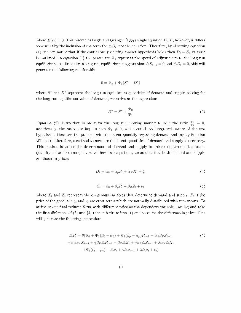
where E(εt) = 0. This resembles Engle and Granger (1987) single equation ECM, however, it di�ers

somewhat by the inclusion of the term the4Dt into the equation. Therefore, by observing equation

(1) one can notice that if the continuously clearing market hypothesis holds then Dt = St,∀t mustbe satis�ed. In equation (1) the parameter Ψ1 represent the speed of adjustments to the long run

equilibrium. Additionally, a long run equilibrium suggests that 4St−1 = 0 and 4Dt = 0, this will

generate the following relationship:

0 = Ψo + Ψ1(S∗ −D∗)

where S∗ and D∗ represent the long run equilibrium quantities of demand and supply, solving for

the long run equilibrium value of demand, we arrive at the expression:

D∗ = S∗ +Ψ0

Ψ1(2)

Equation (2) shows that in order for the long run clearing market to hold the ratio Ψ0

Ψ1= 0,

additionally, the ratio also implies that Ψ1 6= 0, which entails to integrated nature of the two

hypothesis. However, the problem with the latent quantity regarding demand and supply function

still exists; therefore, a method to measure the latent quantities of demand and supply is necessary.

This method is to use the determinants of demand and supply in order to determine the latent

quantity. In order to uniquely solve these two equations, we assume that both demand and supply

are linear in prices:

Dt = α0 + αpPt + αXXt + ζt (3)

St = β0 + βpPt + βZZt + νt (4)

where Xt and Zt represent the exogenous variables that determine demand and supply, Pt is the

price of the good, the ζt and νt are error terms which are normally distributed with zero means. To

arrive at our �nal reduced form with di�erence price as the dependent variable , we lag and take

the �rst di�erence of (3) and (4) then substitute into (1) and solve for the di�erence in price. This

will generate the following expression:

4Pt = θ(Ψ0 + Ψ1(β0 − α0) + Ψ1(βp − αp)Pt−1 + Ψ1βZZt−1 (5)

−Ψ1αXXt−1 + γβP4Pt−1 − βZ4Zt + γβZ4Zt−1 + λαX4Xt

+Ψ1(νt − µt)−4νt + γ4νt−1 + λ4µt + εt)

10

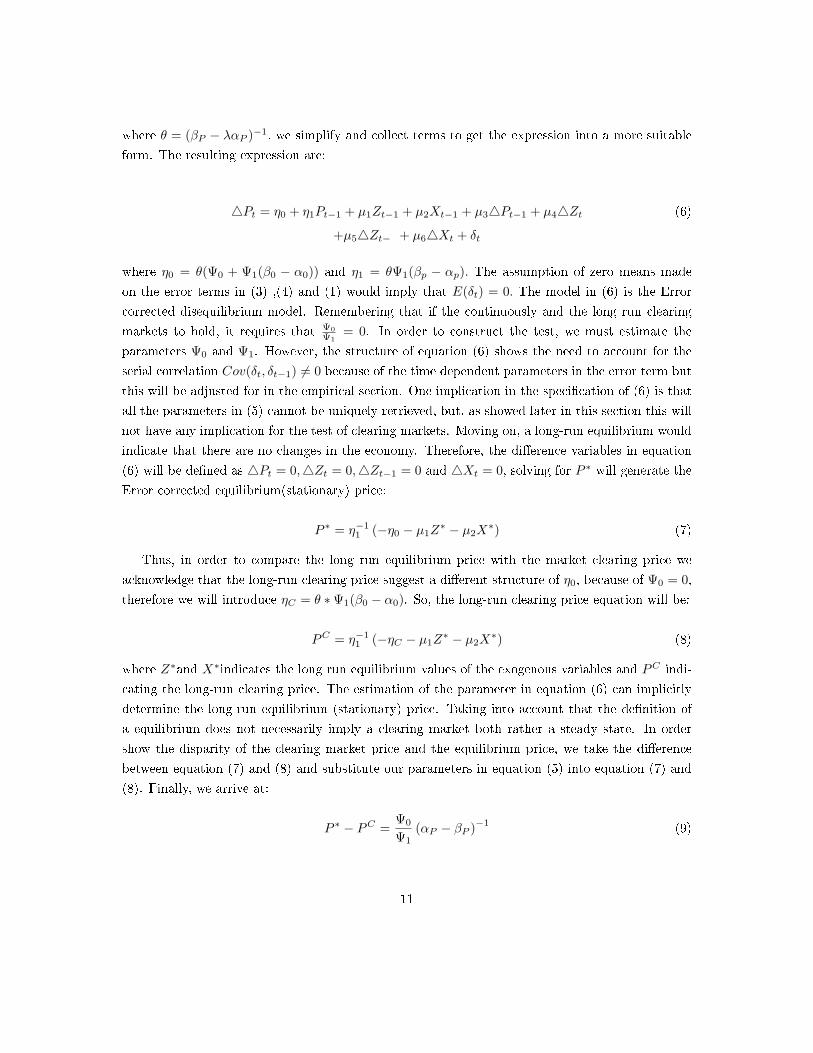
where θ = (βP − λαP )−1, we simplify and collect terms to get the expression into a more suitable

form. The resulting expression are:

4Pt = η0 + η1Pt−1 + µ1Zt−1 + µ2Xt−1 + µ34Pt−1 + µ44Zt (6)

+µ54Zt−1 + µ64Xt + δt

where η0 = θ(Ψ0 + Ψ1(β0 − α0)) and η1 = θΨ1(βp − αp). The assumption of zero means made

on the error terms in (3) ,(4) and (1) would imply that E(δt) = 0. The model in (6) is the Error

corrected disequilibrium model. Remembering that if the continuously and the long run clearing

markets to hold, it requires that Ψ0

Ψ1= 0. In order to construct the test, we must estimate the

parameters Ψ0 and Ψ1. However, the structure of equation (6) shows the need to account for the

serial correlation Cov(δt, δt−1) 6= 0 because of the time dependent parameters in the error term but

this will be adjusted for in the empirical section. One implication in the speci�cation of (6) is that

all the parameters in (5) cannot be uniquely retrieved, but, as showed later in this section this will

not have any implication for the test of clearing markets. Moving on, a long-run equilibrium would

indicate that there are no changes in the economy. Therefore, the di�erence variables in equation

(6) will be de�ned as 4Pt = 0,4Zt = 0,4Zt−1 = 0 and 4Xt = 0, solving for P ∗ will generate the

Error corrected equilibrium(stationary) price:

P ∗ = η−11 (−η0 − µ1Z

∗ − µ2X∗) (7)

Thus, in order to compare the long run equilibrium price with the market clearing price we

acknowledge that the long-run clearing price suggest a di�erent structure of η0, because of Ψ0 = 0,

therefore we will introduce ηC = θ ∗Ψ1(β0 − α0). So, the long-run clearing price equation will be:

PC = η−11 (−ηC − µ1Z

∗ − µ2X∗) (8)

where Z∗and X∗indicates the long run equilibrium values of the exogenous variables and PC indi-

cating the long-run clearing price. The estimation of the parameter in equation (6) can implicitly

determine the long-run equilibrium (stationary) price. Taking into account that the de�nition of

a equilibrium does not necessarily imply a clearing market both rather a steady state. In order

show the disparity of the clearing market price and the equilibrium price, we take the di�erence

between equation (7) and (8) and substitute our parameters in equation (5) into equation (7) and

(8). Finally, we arrive at:

P ∗ − PC =Ψ0

Ψ1(αP − βP )

−1 (9)

11

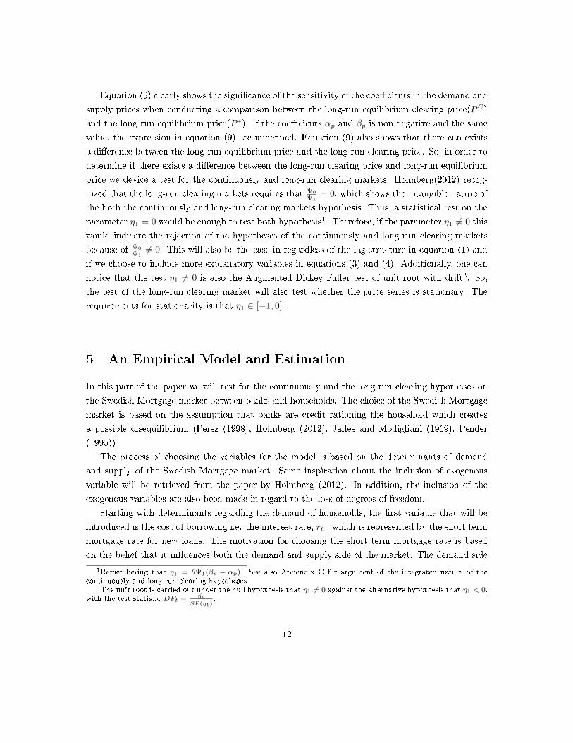
Equation (9) clearly shows the signi�cance of the sensitivity of the coe�cients in the demand and

supply prices when conducting a comparison between the long-run equilibrium clearing price(PC)

and the long-run equilibrium price(P ∗). If the coe�cients αp and βp is non-negative and the same

value, the expression in equation (9) are unde�ned. Equation (9) also shows that there can exists

a di�erence between the long-run equilibrium price and the long-run clearing price. So, in order to

determine if there exists a di�erence between the long-run clearing price and long-run equilibrium

price we device a test for the continuously and long-run clearing markets. Holmberg(2012) recog-

nized that the long-run clearing markets requires that Ψ0

Ψ1= 0, which shows the intangible nature of

the both the continuously and long-run clearing markets hypothesis. Thus, a statistical test on the

parameter η1 = 0 would be enough to test both hypothesis1. Therefore, if the parameter η1 6= 0 this

would indicate the rejection of the hypotheses of the continuously and long-run clearing markets

because of Ψ0

Ψ16= 0. This will also be the case in regardless of the lag structure in equation (1) and

if we choose to include more explanatory variables in equations (3) and (4). Additionally, one can

notice that the test η1 6= 0 is also the Augmented Dickey Fuller test of unit root with drift2. So,

the test of the long-run clearing market will also test whether the price series is stationary. The

requirements for stationarity is that η1 ∈ [−1, 0].

5 An Empirical Model and Estimation

In this part of the paper we will test for the continuously and the long run clearing hypotheses on

the Swedish Mortgage market between banks and households. The choice of the Swedish Mortgage

market is based on the assumption that banks are credit rationing the household which creates

a possible disequilibrium (Perez (1998), Holmberg (2012), Ja�ee and Modigliani (1969), Pender

(1995))

The process of choosing the variables for the model is based on the determinants of demand

and supply of the Swedish Mortgage market. Some inspiration about the inclusion of exogenous

variable will be retrieved from the paper by Holmberg (2012). In addition, the inclusion of the

exogenous variables are also been made in regard to the loss of degrees of freedom.

Starting with determinants regarding the demand of households, the �rst variable that will be

introduced is the cost of borrowing i.e. the interest rate, rt , which is represented by the short term

mortgage rate for new loans. The motivation for choosing the short term mortgage rate is based

on the belief that it in�uences both the demand and supply side of the market. The demand side

1Remembering that η1 = θΨ1(βp − αp). See also Appendix C for argument of the integrated nature of thecontinuously and long-run clearing hypotheses

2The unit root is carried out under the null hypothesis that η1 6= 0 against the alternative hypothesis that η1 < 0,with the test statistic DFt = η̂1

SE( ˆη1).

12

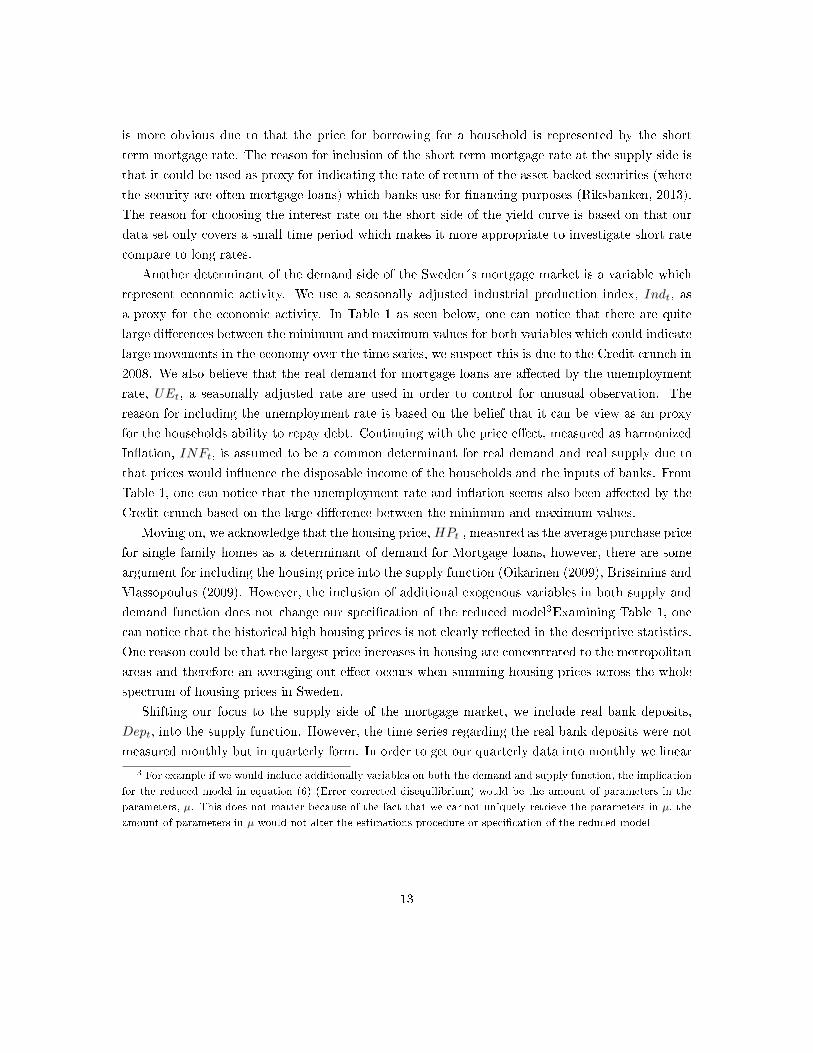
is more obvious due to that the price for borrowing for a household is represented by the short

term mortgage rate. The reason for inclusion of the short term mortgage rate at the supply side is

that it could be used as proxy for indicating the rate of return of the asset backed securities (where

the security are often mortgage loans) which banks use for �nancing purposes (Riksbanken, 2013).

The reason for choosing the interest rate on the short side of the yield curve is based on that our

data set only covers a small time period which makes it more appropriate to investigate short rate

compare to long rates.

Another determinant of the demand side of the Sweden´s mortgage market is a variable which

represent economic activity. We use a seasonally adjusted industrial production index, Indt, as

a proxy for the economic activity. In Table 1 as seen below, one can notice that there are quite

large di�erences between the minimum and maximum values for both variables which could indicate

large movements in the economy over the time series, we suspect this is due to the Credit crunch in

2008. We also believe that the real demand for mortgage loans are a�ected by the unemployment

rate, UEt, a seasonally adjusted rate are used in order to control for unusual observation. The

reason for including the unemployment rate is based on the belief that it can be view as an proxy

for the households ability to repay debt. Continuing with the price e�ect, measured as harmonized

In�ation, INFt, is assumed to be a common determinant for real demand and real supply due to

that prices would in�uence the disposable income of the households and the inputs of banks. From

Table 1, one can notice that the unemployment rate and in�ation seems also been a�ected by the

Credit crunch based on the large di�erence between the minimum and maximum values.

Moving on, we acknowledge that the housing price, HPt , measured as the average purchase price

for single family homes as a determinant of demand for Mortgage loans, however, there are some

argument for including the housing price into the supply function (Oikarinen (2009), Brissimins and

Vlassopoulus (2009). However, the inclusion of additional exogenous variables in both supply and

demand function does not change our speci�cation of the reduced model3Examining Table 1, one

can notice that the historical high housing prices is not clearly re�ected in the descriptive statistics.

One reason could be that the largest price increases in housing are concentrated to the metropolitan

areas and therefore an averaging out e�ect occurs when summing housing prices across the whole

spectrum of housing prices in Sweden.

Shifting our focus to the supply side of the mortgage market, we include real bank deposits,

Dept, into the supply function. However, the time series regarding the real bank deposits were not

measured monthly but in quarterly form. In order to get our quarterly data into monthly we linear

3 For example if we would include additionally variables on both the demand and supply function, the implication

for the reduced model in equation (6) (Error corrected disequilibrium) would be the amount of parameters in the

parameters, µ. This does not matter because of the fact that we cannot uniquely retrieve the parameters in µ, the

amount of parameters in µ would not alter the estimations procedure or speci�cation of the reduced model

13

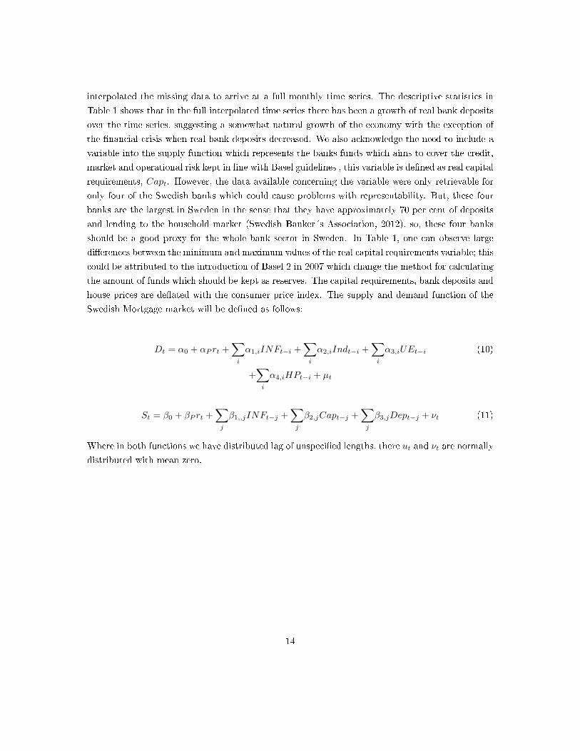
interpolated the missing data to arrive at a full monthly time series. The descriptive statistics in

Table 1 shows that in the full interpolated time series there has been a growth of real bank deposits

over the time series, suggesting a somewhat natural growth of the economy with the exception of

the �nancial crisis when real bank deposits decreased. We also acknowledge the need to include a

variable into the supply function which represents the banks funds which aims to cover the credit,

market and operational risk kept in line with Basel guidelines , this variable is de�ned as real capital

requirements, Capt. However, the data available concerning the variable were only retrievable for

only four of the Swedish banks which could cause problems with representability. But, these four

banks are the largest in Sweden in the sense that they have approximately 70 per cent of deposits

and lending to the household market (Swedish Banker´s Association, 2012), so, these four banks

should be a good proxy for the whole bank sector in Sweden. In Table 1, one can observe large

di�erences between the minimum and maximum values of the real capital requirements variable; this

could be attributed to the introduction of Basel 2 in 2007 which change the method for calculating

the amount of funds which should be kept as reserves. The capital requirements, bank deposits and

house prices are de�ated with the consumer price index. The supply and demand function of the

Swedish Mortgage market will be de�ned as follows:

Dt = α0 + αP rt +∑i

α1,iINFt−i +∑i

α2,iIndt−i +∑i

α3,iUEt−i (10)

+∑i

α4,iHPt−i + µt

St = β0 + βP rt +∑j

β1,,jINFt−j +∑j

β2,jCapt−j +∑j

β3,jDept−j + νt (11)

Where in both functions we have distributed lag of unspeci�ed lengths, there ut and νt are normally

distributed with mean zero.

14

The data regarding the Swedish Mortgage market is aggregate monthly data from October 2005 to

December 2012, retrieved from Statistics of Sweden and Datastream (Database regarding �nancial

data).

Table 1. Descriptive Statistics

Variable Mean Std.Dev Min MaxShort term mortgage rate (rt) 3.442 1.190 1.51 6.1

Industrial production Index (Indt) 104.684 11.798 70.7 127.6Unemployment rate (UEt) 7.408 0.838 5.5 9.5Real housing price (HPt) 1.744 0.120 1.358 2.031

In�ation ( INFt) 1.615 1.407 -1.9 4.4Real deposits ( Dept) 1794410 259437.5 1218659 2216032

Real capital requirements ( Capt) 102.976 27.437 42.951 158.107

Note: rt, UEt and INFt are measured in per cent whilst HPt,Dept and Capt are measured inMillion SEK

So, the Credit crunch has a�ected both the demand and supply sides of the Swedish Mortgage

market. Therefore, the Credit crunch should be accounted for, based on this we use two di�erent

indicator for this event. The �rst indicator recognize the historical lowering of the prime rate

between December 2008 to July 2009, so, we construct the indicator variable, I2009t , for the year

2009. Continuing with the second indicator variable, we acknowledge the origin of the Credit crunch

as the Lehman´s Brothers Crash in 2008, thus, creating a indicator for 2008, I2008t . The use of

two indicators will produce two di�erent models for comparison. We will also split our sample into

two di�erent parts, i.e. pre-and post recession, but keeping the same structure of the models as

the full model with exception of the indicator variable. The split consists of recognizing that the

major impact of the �nancial crisis came into e�ect in 2009, therefore, removing this year for these

reduced models in order to compare estimates before and after recession. Notable, this will only be

applied with our �rst full model with the indicator, I2009t . These full models will be based on the

speci�cation in equation (6).

In order to estimate our parameters e�ciently and consistently, we need to acknowledge the

need to adjust for Cov(δt, δt−i) 6= 0 because of inherent structure of the model and the nature of

the data. To con�rm the presence of autocorrelation we use a Box-Pierce Portmanteau test. The

null hypothesis is that the error term could be seen as white noise. The results showed that we

can reject the hypothesis of white noise, therefore, con�rming our belief of autocorrelation. Based

on the premises of Holmberg (2012), we test the hypothesis of possible conditional heteroskedastic-

ity. Using the Breusch-Pagan / Cook-Weisberg test, we �nd evidence of heteroskedasticity in our

15

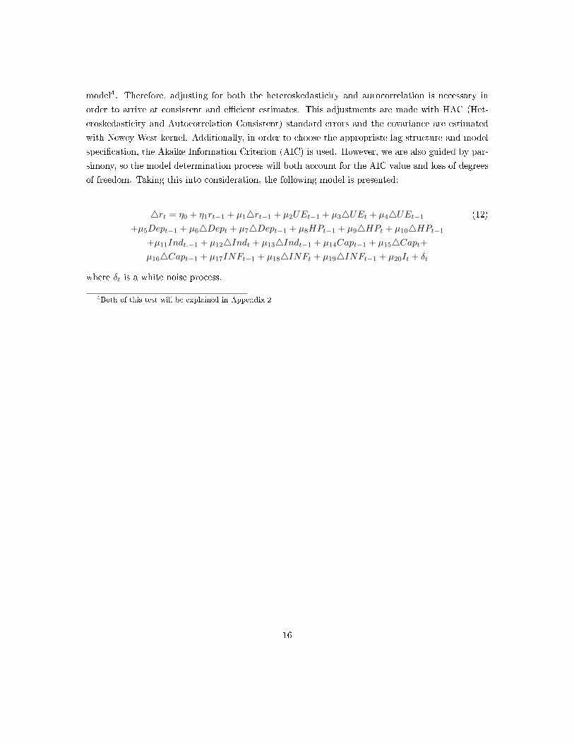
model4. Therefore, adjusting for both the heteroskedasticity and autocorrelation is necessary in

order to arrive at consistent and e�cient estimates. This adjustments are made with HAC (Het-

eroskedasticity and Autocorrelation Consistent) standard errors and the covariance are estimated

with Newey-West kernel. Additionally, in order to choose the appropriate lag structure and model

speci�cation, the Akaike Information Criterion (AIC) is used. However, we are also guided by par-

simony, so the model determination process will both account for the AIC value and loss of degrees

of freedom. Taking this into consideration, the following model is presented:

4rt = η0 + η1rt−1 + µ14rt−1 + µ2UEt−1 + µ34UEt + µ44UEt−1 (12)

+µ5Dept−1 + µ64Dept + µ74Dept−1 + µ8HPt−1 + µ94HPt + µ104HPt−1

+µ11Indt.−1 + µ124Indt + µ134Indt−1 + µ14Capt−1 + µ154Capt+µ164Capt−1 + µ17INFt−1 + µ184INFt + µ194INFt−1 + µ20It + δt

where δt is a white noise process.

4Both of this test will be explained in Appendix 2

16

5.1 Results

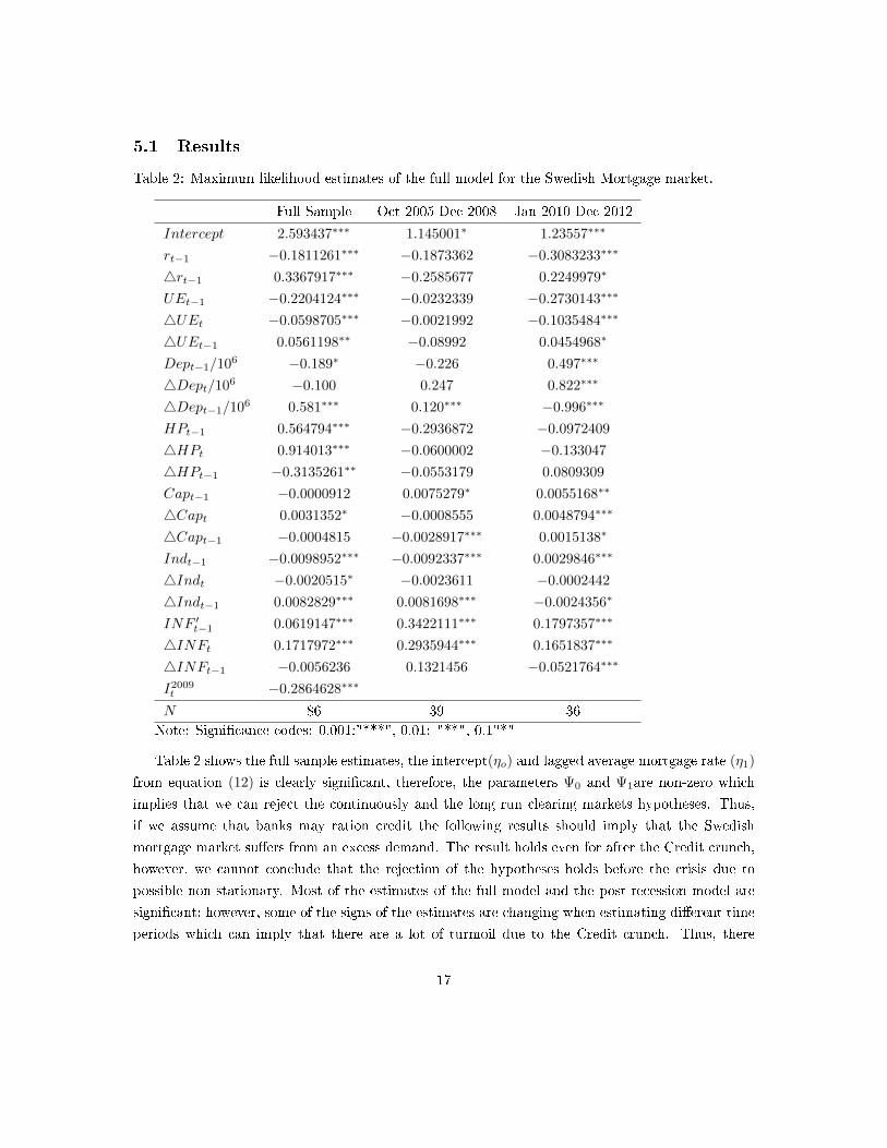
Table 2: Maximum likelihood estimates of the full model for the Swedish Mortgage market.

Full Sample Oct 2005-Dec 2008 Jan 2010-Dec 2012

Intercept 2.593437∗∗∗ 1.145001∗ 1.23557∗∗∗

rt−1 −0.1811261∗∗∗ −0.1873362 −0.3083233∗∗∗

4rt−1 0.3367917∗∗∗ −0.2585677 0.2249979∗

UEt−1 −0.2204124∗∗∗ −0.0232339 −0.2730143∗∗∗

4UEt −0.0598705∗∗∗ −0.0021992 −0.1035484∗∗∗

4UEt−1 0.0561198∗∗ −0.08992 0.0454968∗

Dept−1/106 −0.189∗ −0.226 0.497∗∗∗

4Dept/106 −0.100 0.247 0.822∗∗∗

4Dept−1/106 0.581∗∗∗ 0.120∗∗∗ −0.996∗∗∗

HPt−1 0.564794∗∗∗ −0.2936872 −0.0972409

4HPt 0.914013∗∗∗ −0.0600002 −0.133047

4HPt−1 −0.3135261∗∗ −0.0553179 0.0809309

Capt−1 −0.0000912 0.0075279∗ 0.0055168∗∗

4Capt 0.0031352∗ −0.0008555 0.0048794∗∗∗

4Capt−1 −0.0004815 −0.0028917∗∗∗ 0.0015138∗

Indt−1 −0.0098952∗∗∗ −0.0092337∗∗∗ 0.0029846∗∗∗

4Indt −0.0020515∗ −0.0023611 −0.0002442

4Indt−1 0.0082829∗∗∗ 0.0081698∗∗∗ −0.0024356∗

INF ′t−1 0.0619147∗∗∗ 0.3422111∗∗∗ 0.1797357∗∗∗

4INFt 0.1717972∗∗∗ 0.2935944∗∗∗ 0.1651837∗∗∗

4INFt−1 −0.0056236 0.1321456 −0.0521764∗∗∗

I2009t −0.2864628∗∗∗

N 86 39 36Note: Signi�cance codes: 0.001:"***", 0.01: "**", 0.1"*"

Table 2 shows the full sample estimates, the intercept(ηo) and lagged average mortgage rate (η1)

from equation (12) is clearly signi�cant, therefore, the parameters Ψ0 and Ψ1are non-zero which

implies that we can reject the continuously and the long run clearing markets hypotheses. Thus,

if we assume that banks may ration credit the following results should imply that the Swedish

mortgage market su�ers from an excess demand. The result holds even for after the Credit crunch,

however, we cannot conclude that the rejection of the hypotheses holds before the crisis due to

possible non-stationary. Most of the estimates of the full model and the post-recession model are

signi�cant; however, some of the signs of the estimates are changing when estimating di�erent time

periods which can imply that there are a lot of turmoil due to the Credit crunch. Thus, there

17

are a possible that the turmoil is spilling over to other years than 2009. One can also notice that

η1 ∈ [−1, 0] for the full model, so, this concludes that the price series is also a stationary process.

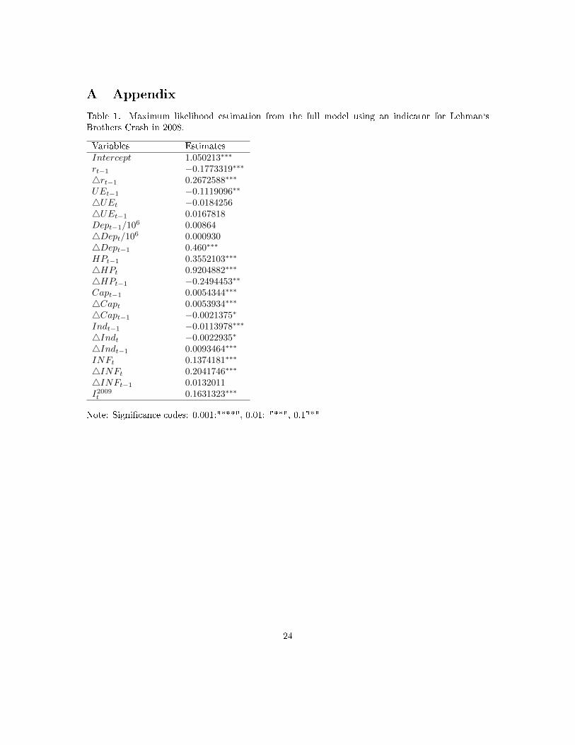
Results from the estimation of the second model with the indicator, I2008t (see appendix 1, Table

1) also indicates that we can reject the hypotheses of continuously and long-run clearing markets.

Therefore, suggesting the possibility of a disequilibrium. As seen in in Appendix A Table 1, the

overall signi�cans of the estimates suggests a good �t, additionally, most all of the estimates have the

expected signs. The AIC value for the second model with the indicator for the Lehman`s Brothers

Crash is higher than the value of the �rst models, therefore, suggesting that the �rst model is

a better �t than the second. Thus, the model with Lehman´s Brothers Crash indicator explain

less than our model with the indicator for the historical lowering of the prime rate. However, this

could seem reasonable due to lagged e�ect of the �nancial collapse on the Swedish mortgage market

regarding the mortgage rate.

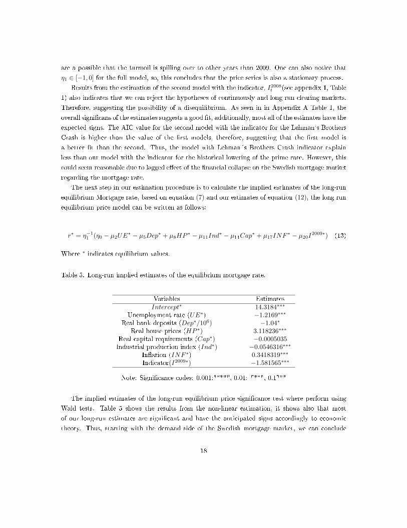
The next step in our estimation procedure is to calculate the implied estimates of the long-run

equilibrium Mortgage rate, based on equation (7) and our estimates of equation (12), the long run

equilibrium price model can be written as follows:

r∗ = η−11 (η0 − µ2UE

∗ − µ5Dep∗ + µ8HP

∗ − µ11Ind∗ − µ14Cap∗ + µ17INF

∗ − µ20I2009∗) (13)

Where ∗ indicates equilibrium values.

Table 5. Long-run implied estimates of the equilibrium mortgage rate.

Variables EstimatesIntercept∗ 14.3184∗∗∗

Unemployment rate (UE∗) −1.2169∗∗∗

Real bank deposits (Dep∗/106) −1.04∗

Real house prices (HP ∗) 3.118236∗∗∗

Real capital requirements (Cap∗) −0.0005035Industrial production index (Ind∗) −0.0546316∗∗∗

In�ation (INF ∗) 0.3418319∗∗∗

Indicator(I2009∗) −1.581565∗∗∗

Note: Signi�cance codes: 0.001:"***", 0.01: "**", 0.1"*"

The implied estimates of the long-run equilibrium price signi�cance test where perform using

Wald tests. Table 5 shows the results from the non-linear estimation, it shows also that most

of our long-run estimates are signi�cant and have the anticipated signs accordingly to economic

theory. Thus, starting with the demand side of the Swedish mortgage market, we can conclude

18

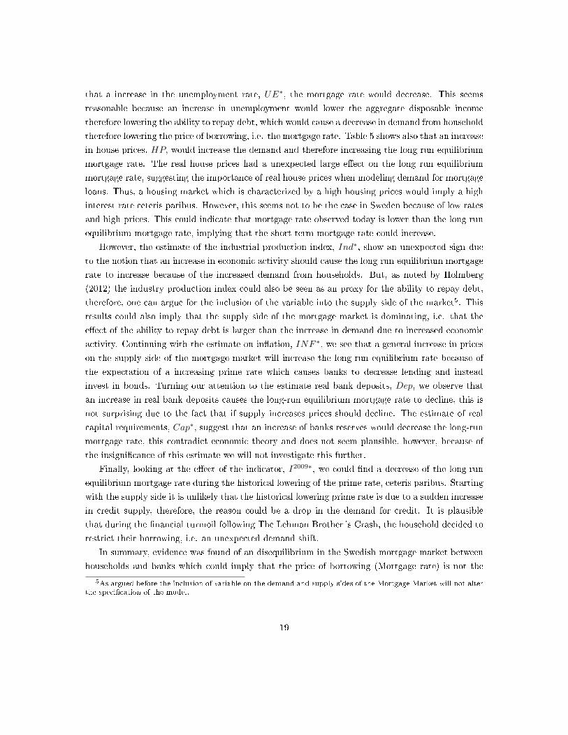
that a increase in the unemployment rate, UE∗, the mortgage rate would decrease. This seems

reasonable because an increase in unemployment would lower the aggregate disposable income

therefore lowering the ability to repay debt, which would cause a decrease in demand from household

therefore lowering the price of borrowing, i.e. the mortgage rate. Table 5 shows also that an increase

in house prices, HP, would increase the demand and therefore increasing the long run equilibrium

mortgage rate. The real house prices had a unexpected large e�ect on the long run equilibrium

mortgage rate, suggesting the importance of real house prices when modeling demand for mortgage

loans. Thus, a housing market which is characterized by a high housing prices would imply a high

interest rate ceteris paribus. However, this seems not to be the case in Sweden because of low rates

and high prices. This could indicate that mortgage rate observed today is lower than the long run

equilibrium mortgage rate, implying that the short term mortgage rate could increase.

However, the estimate of the industrial production index, Ind∗, show an unexpected sign due

to the notion that an increase in economic activity should cause the long run equilibrium mortgage

rate to increase because of the increased demand from households. But, as noted by Holmberg

(2012) the industry production index could also be seen as an proxy for the ability to repay debt,

therefore, one can argue for the inclusion of the variable into the supply side of the market5. This

results could also imply that the supply side of the mortgage market is dominating, i.e. that the

e�ect of the ability to repay debt is larger than the increase in demand due to increased economic

activity. Continuing with the estimate on in�ation, INF ∗, we see that a general increase in prices

on the supply side of the mortgage market will increase the long-run equilibrium rate because of

the expectation of a increasing prime rate which causes banks to decrease lending and instead

invest in bonds. Turning our attention to the estimate real bank deposits, Dep, we observe that

an increase in real bank deposits causes the long-run equilibrium mortgage rate to decline, this is

not surprising due to the fact that if supply increases prices should decline. The estimate of real

capital requirements, Cap∗, suggest that an increase of banks reserves would decrease the long-run

mortgage rate, this contradict economic theory and does not seem plausible, however, because of

the insigni�cance of this estimate we will not investigate this further.

Finally, looking at the e�ect of the indicator, I2009∗, we could �nd a decrease of the long-run

equilibrium mortgage rate during the historical lowering of the prime rate, ceteris paribus. Starting

with the supply side it is unlikely that the historical lowering prime rate is due to a sudden increase

in credit supply, therefore, the reason could be a drop in the demand for credit. It is plausible

that during the �nancial turmoil following The Lehman Brother´s Crash, the household decided to

restrict their borrowing, i.e. an unexpected demand shift.

In summary, evidence was found of an disequilibrium in the Swedish mortgage market between

households and banks which could imply that the price of borrowing (Mortgage rate) is not the

5As argued before the inclusion of variable on the demand and supply sides of the Mortgage Market will not alterthe speci�cation of the model.

19

market clearing price. The estimation results showed also that most of the estimates regarding

determinants of supply and demand of the Mortgage market show anticipated signs and a overall

signi�cance.

6 Conclusions

The main purpose of this paper was to investigate the existence of disequilibrium on the Swedish

mortgage market between households and banks. Using the framework derived by Holmberg (2012)

in his Error corrected disequilibrium model which accounted for both the cointegration of the de-

mand and supply function and possible nonstationarity. Using this model we could �nd tests which

examine both the hypotheses of continuously and long-run clearing market. The models were esti-

mated with maximum likelihood method adjusting for both heteroskedasticity and autocorrelation;

we apply these tests to the Swedish Mortgage market with data collected between 2005-2012. The

results showed that both hypotheses could be rejected suggesting that the Swedish mortgage market

is su�ering from disequilibrium.

Therefore, a possible disequilibrium implies that the observable price is not the market clearing

price which suggests a ine�ciency on the market. The low prime rate and the proposed credit

rationing by banks suggests that the market is su�ering from a excess demand (Stiglietz and Weiss

(1981), Holmberg (2012)). An implication of this relative long period with a low mortgage rate in a

disequilibrium state could be that households forms expectations about the future short term mort-

gage rate which could be lower than the true long-run equilibrium mortgage rate. One consequence

of this could be that it induces household to borrow more, which could also have the implication

that interest movements causes a larger e�ect in household´s economy. Results from the estimation

of the models support this claim, based on that an increase in house prices would indicate fairly

large increase in the long-run equilibrium short term mortgage rate. However, comparing this result

to the situation in the housing market today with high house prices and a low short term mortgage

rate, suggests that the rate to observed today is much lower than the long-run equilibrium short

term mortgage rate which could imply that the short term mortgage would increase. The problem

with proposed change of households expectations regarding the mortgage rate in combination with

banks disparity in respect to loan requirements could be reasons to argue for the existence of a

housing bubble.

However, as described in the "Housing bubbles and �nancial fragility" section, Sweden´s pro-

posed bubble in the housing market di�ers to other bubbles, this di�erence is mainly due to low

construction and high savings. It is hard to point to a certain factor as the main factor which causes

a bubble and even harder to determine if there is bubble or not. Nevertheless, there is a need to

implement di�erent measures to try to lower the households willingness to borrow in order to get

a normalized development of the house prices. The prime rate is an e�cient measure; however, the

20

in�ation is nearly zero suggesting the prime rate as a bad instrument for this purposes. Therefore,

there is a need for new legislative procedure regarding more stringent requirements of receiving a

mortgage loan in order to cool down the housing market.

7 Ackknowledgement

I want to thank my supervisor Tomas Sjögren for all the advice and guidence when writing thisthesis.

21

8 References

ADAMS, Z. AND F.FÜSS (2010): "Macroeconomic determinants of international housing markets,"

Journal of Housing Economics 19, 38-50.

ALSTERLIND, J ET. AL (2014): "PM 6 - Risker för makroekonomin och den �nansiella stabiliteten

av utvecklingen av hushållens skulder och bostadspriserna," Riksbanken, 1-36.

ABRAHAM, J.M AND P.H HENDERSHOTT (1994): "Bubbles In Metropolitan Housing Mar-

kets," National Bureau of Economic Research, 1-27.

BOWDEN, R. J. (1978): "Speci�cation, Estimation and Inference for Models of Markets in Dise-

quilibrium," International Economic Review, 19, 711�726.

BARRO, R.J. AND H.I Grossman (1971): "A General Disequilibrium Model of Income and Em-

ployment". American Economic Review, 82-93.

BYUN, K. J. (2010): "The U.S. Housing Bubble and Bust: Impacts on Employment," Monthly

Labor Review, 3-17.

CLAUSSEN, C.A. ET AL (2011): "En Makroekonomisk Analys av Bostadspriserna i Sverige,"

Riksbankens utredning om risker på den svenska bostadsmarknaden, 67-173.

ENGLE, R. F. AND C. W. J. GRANGER (1987): "Co-integration and Error Correction: Repre-

sentation, Estimation, and Testing," Econometrica, 55, 251�276.

FAIR, R. C. AND D. M. JAFFEE (1972): "Methods of Estimation for Markets in Disequilibrium,"

Econometrica, 40, 497�514.

FINANSINSPEKTIONEN (2013): "Den Svenska Bolånemarknaden,", 1-22.

GENTIER, A. (2012): "Spanish Banks and the Housing Crisis: Worse than the Subprime Crisis?"

International Journal of Business, 17(4), 343-353.

GRANGER, C. W. J. AND P. NEWBOLD (1974): "Spurious Regressions in Econometrics," Jour-

nal of Econometrics, 2, 111�120.

GREENWALD, B.C. AND J.E. STIGLITZ (1990): "Macroeconomic Models with Equity and

Credit Rationing," National Bureau of Economic Research, 15-42.

HOLMBERG, U. (2012):" Error Corrected Disequilibrium," Ph.D. thesis, Umeå School of Business

and Economics.

22

HORT, K. (1998):"The Determinants of Urban House Price Fluctuations in Sweden 1968- 1994,"

Journal of Housing Economics, 7, 93-120.

HURLIN, C. AND R. KIERZENKOWSKI (2003): "Credit Market Disequilibrium in Poland: Can

We Find What We Expect? Non-Stationarity and the "Min" Condition," William Davidson Insti-

tute Working Papers Series 2003-581, William Davidson Institute at the University of Michigan.

JAFFEE, D. M AND F. Modigliani (1969): "A theory and test of credit rationing," The American

Economic Review ,59 no. 5, 850-872.

LAFFONT, J.-J. AND R. GARCIA (1977): "Disequilibrium Econometrics for Business Loans,"

Econometrica, 45, 1187�1204.

MADDALA, G. S. AND F. D. NELSON (1974): "Maximum Likelihood Methods for Models of

Markets in Disequilibrium," Econometrica, 42, 1013�1030.

OIKARINEN, E. (2009): "Interaction between Housing prices and Household borrowing: The

Finnish Case," Journal of Banking and Finance ,33, 747-756.

PEREZ, S. J. (1998): "Testing for Credit Rationing: An Application of Disequilibrium Economet-

rics," Journal of Macroeconomics, 20, 721�739.

SIEBERT, H. (1997): "Labor Market Rigidities and Unemployment in Europe," Kiel Working

Paper ,No. 787, 2-25.

STIGLITZ, J. E. AND A. WEISS (1981): "Credit Rationing in Markets with Imperfect Informa-

tion," The American Economic Review, 71, 393�410.

SWEDISH BANKERS ASSOCIATION (2013), "Bank and Finance Statistics,". 3-12.

QUANDT, R.E.(1958): "The Estimation of the Parameters of a Linear Regression System ObeyingTwo Separate Regimes," Journal of the American Statistical Association, 53, 873-880.

23

A Appendix

Table 1. Maximum likelihood estimation from the full model using an indicator for Lehman`sBrothers Crash in 2008.

Variables EstimatesIntercept 1.050213∗∗∗

rt−1 −0.1773319∗∗∗

4rt−1 0.2672588∗∗∗

UEt−1 −0.1119096∗∗

4UEt −0.01842564UEt−1 0.0167818Dept−1/106 0.008644Dept/106 0.0009304Dept−1 0.460∗∗∗

HPt−1 0.3552103∗∗∗

4HPt 0.9204882∗∗∗

4HPt−1 −0.2494453∗∗

Capt−1 0.0054344∗∗∗

4Capt 0.0053934∗∗∗

4Capt−1 −0.0021375∗

Indt−1 −0.0113978∗∗∗

4Indt −0.0022935∗

4Indt−1 0.0093464∗∗∗

INFt 0.1374181∗∗∗

4INFt 0.2041746∗∗∗

4INFt−1 0.0132011I2009t 0.1631323∗∗∗

Note: Signi�cance codes: 0.001:"***", 0.01: "**", 0.1"*"

24

B Appendix

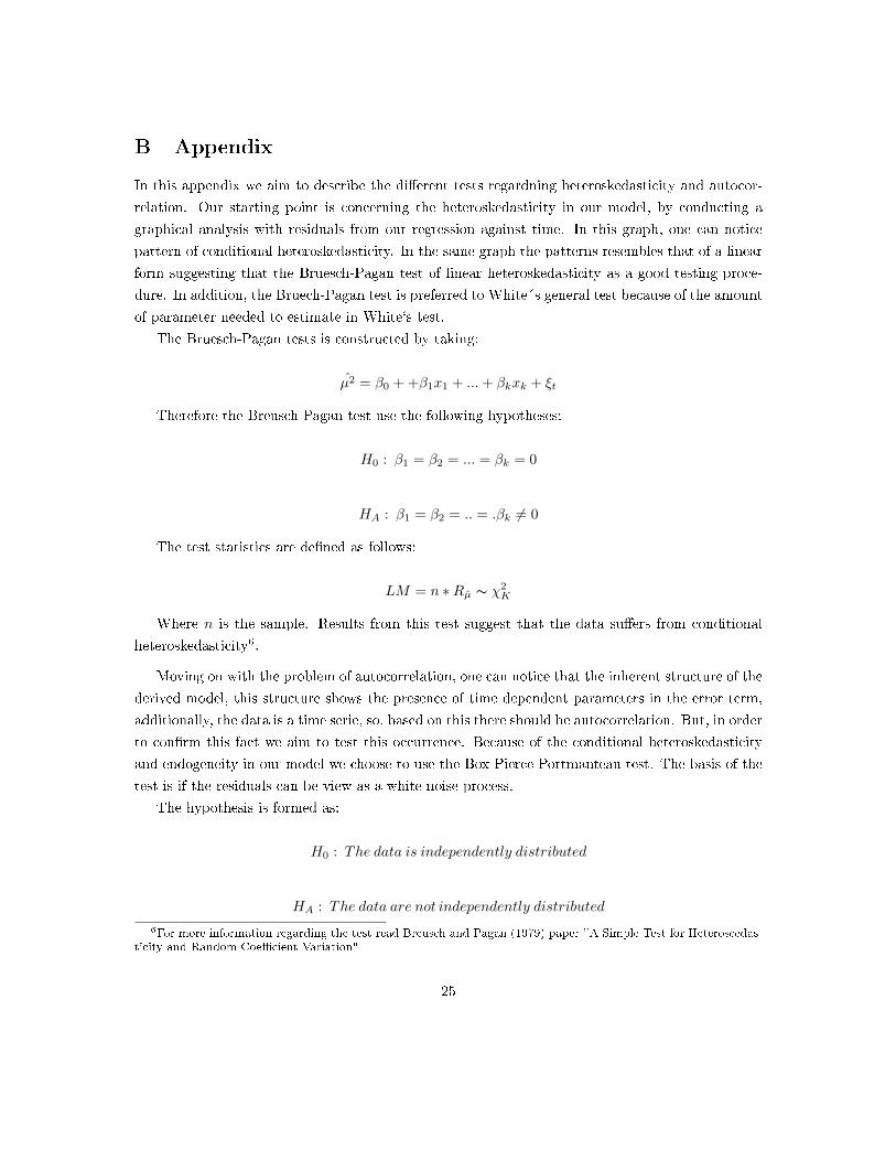
In this appendix we aim to describe the di�erent tests regardning heteroskedasticity and autocor-

relation. Our starting point is concerning the heteroskedasticity in our model, by conducting a

graphical analysis with residuals from our regression against time. In this graph, one can notice

pattern of conditional heteroskedasticity. In the same graph the patterns resembles that of a linear

form suggesting that the Bruesch-Pagan test of linear heteroskedasticity as a good testing proce-

dure. In addition, the Bruech-Pagan test is preferred to White´s general test because of the amount

of parameter needed to estimate in White`s test.

The Bruesch-Pagan tests is constructed by taking:

µ̂2 = β0 + +β1x1 + ...+ βkxk + ξt

Therefore the Breusch-Pagan test use the following hypotheses:

H0 : β1 = β2 = ... = βk = 0

HA : β1 = β2 = .. = .βk 6= 0

The test statistics are de�ned as follows:

LM = n ∗Rµ̂ ∼ χ2K

Where n is the sample. Results from this test suggest that the data su�ers from conditional

heteroskedasticity6.

Moving on with the problem of autocorrelation, one can notice that the inherent structure of the

derived model, this structure shows the presence of time dependent parameters in the error term,

additionally, the data is a time serie, so, based on this there should be autocorrelation. But, in order

to con�rm this fact we aim to test this occurrence. Because of the conditional heteroskedasticity

and endogeneity in our model we choose to use the Box-Pierce Portmanteau test. The basis of the

test is if the residuals can be view as a white noise process.

The hypothesis is formed as:

H0 : The data is independently distributed

HA : The data are not independently distributed

6For more information regarding the test read Breusch and Pagan (1979) paper "A Simple Test for Heteroscedas-ticity and Random Coe�cient Variation"

25

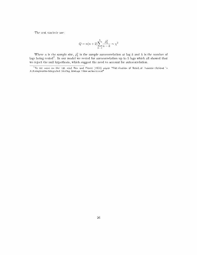
The test statistic are:

Q = n(n+ 2)

h∑k−1

ρ̂2k

n− k∼ χ2

Where n is the sample size, ρ̂2k is the sample autocorrelation at lag k and h is the number of

lags being tested7. In our model we tested for autocorrelation up to 5 lags which all showed thatwe reject the null hypothesis, which suggest the need to account for autocorrelation.

7To see more on the test read Box and Pierce (1970) paper "Distribution of Residual Autocorrelations inAutoregressive-Integrated Moving Average Time series model"

26

C Appendix

In this appendix we aim to explain the logic behind the single statistical test of the parameter

η1 and the integrated hypotheses of the continuously and long-run clearing markets. Much of the

notation and derivation will be retrieved from Holmberg (2012). In order to explain the integrated

nature of both hypotheses, we start from the long-run clearing markets, which test is based on the

parameters η0 and η1 derived from Error corrected disequilibrium model in equation (6). By �rst

looking at the compounded parameters of the parameter η1:

η1 = Ψ1

(βp − αpβp − λαp

)(C.1)

assuming that the price sensitivity of demand and supply sides will di�ers, which implies that

βp 6= αp . Therefore, following this argument a non-zero value on η1 suggest a non-zero value on

Ψ1. One implication of Ψ1 6= 0 is the rejection the continuously clearing hypothesis.

Moving on to the long-run clearing markets hypothesis, if the clearing market assumption were

to hold this would indicate that Ψ0

Ψ1= 0. Thus, there is need to �nd some measurable implication

of this ratio. As shown by Holmberg (2012), a non-zero value on η1 implies a non-zero value of the

ratio. Proving this statement, we use the intercept from equation (6):

η0 =Ψ0 + Ψ1(β0 − αo)

βp − λαp(C.2)

consider a case where η0 = 0 and we were solve for Ψ0 in (C.2):

Ψ0 = Ψ1(α0 − β0) (C.3)

Equation (C.3) states that if the long-run clearing market assumption to hold it requires that

α0 = β0 under the assumption that η1 6= 0 which implies that Ψ1 6= 0. These cases where α0 = β0

are not relevant. The same arguments holds if we let η0 6= 0. In order to show this scenario, we set

Ψ0 = 0 in (C.2), solving the equation for Ψ1 we arrive at:

Ψ1 = η0

(βp − λαpβ0 − α0

)(C.4)

if we solve also for Ψ1 in equation (C.1) and remember the assumption that the price sensitivities

of demand and supply di�ers (αp 6= βP ):

27

Ψ1 = η1

(βp − λαPβp − αP

)(C.5)

Substituting in (C.5) into (C.4) and solve for λ:

λ =βPαP

(C.6)

if we were to substitute this back into (C.4), one can conclude that this would imply that Ψ1 = 0.

This implies for (C.1) that η1 = 0 if Ψ0 = 0 when η0 6= 0. Therefore, if η1 6= 0 and η0 6= 0 this

would mean that Ψ0 is non-zero and we can reject the long-run clearing markets assumption.

The results from this derivation shows that a statistical test on parameter η1 would su�ce in

order to test both the continuously and long-run clearing market hypotheses. Because of the fact

that clearing market in the long-run is necessary condition for the continuously clearing market

hypothesis.

28