A detailed discussion of superfield supergravity prepotential perturbations

arX

iv:0

909.

0294

v2 [

hep-

th]

24

Jul 2

010

A detailed discussion of superfield

supergravity prepotential perturbations

in the superspace of the

AdS5/CFT4 correspondence

J. Ovalle∗

Departamento de Fısica,Universidad Simon Bolıvar,

Caracas, Venezuela.

Abstract

This paper presents a detailed discussion of the issue of supergra-vity perturbations around the flat five dimensional superspace re-quired for manifest superspace formulations of the supergravity sideof the AdS5/CFT4 Correspondence.

pacs 04.65.+e

∗[email protected]

1

1 Introduction

The importance of deeply understanding the superspace geometry of five

dimensions, has received attention during the last few years [1], [2], [3], mo-

tivated mainly by the postulate of the AdS/CFT correspondence [4]. In this

respect, the study of supergravity theories represents an unavoidable issue

[5], [6], [7], even more keeping in mind the existence of the supergravity side

of the AdS5/CFT4 correspondence. Indeed the works of [6, 7] present com-

plete nonlinear descriptions of such superspaces based on a particular choice

of compensators. It has long been known [8], that the superspace geometry

changes when different compensators are introduced. So one of the goals of

the current study is to begin the process of looking at what features of the

work of [6, 7] are universal (i.e. independent of compensator choice).

When the superspace approach is used, the conventional representation

for Grassmann variables for SUSY D = 5, N = 1 (often denominated

N = 2) considers these variables obeying a pseudo-Majorana reality condi-

tion, then the spinor coordinates are dotted with an SU(2) index. Thus the

conventional approach first doubles the number of fermionic coordinates, by

the introduction of the SU(2) index, then halves this number by the imposi-

tion of the pseudo-Majorana reality condition. However, as noted previously

[1], there is no fundamental principle that demands the use of Majorana-

symplectic spinors for describing the fermionic coordinated. Indeed, it was

demonstrated in [1] that complex 4-components spinors provide an adequate

basis for describing such a fermionic coordinate. Building on this previous

work, in this paper it will be shown that it is possible to develop successfully

a geometrical approach to five dimensional N = 1 supergravity theory, using

this unconventional representation for Grassmann variables.

The geometrical approach to supergravity involves calculating fields

strengths to determine the form of the torsions and curvatures of the the-

ory. With this information in hand, we can set constraints such that the

super spin connections and the vector-supervector component of the inverse

supervierbein become dependent variables of the theory. Once this is accom-

plished, the route to deducing the prepotentials of the supergravity theory are

opened. On the other hand, there is an alternative approach which is based

in the torsion superfield C CAB associated to the superspace derivative EA,

2

namely, the super-anholonomy [EA, EB} = C CAB EC . Using the superspace

derivative ∇A to calculate the super (anti)-commutator [∇A,∇B}, we will be

able to write all super-torsion components in terms of the anholonomy and

the spinorial connection. Through a choice of suitable constraints on super-

space through some super-torsion components, we will be able to write the

spin connection superfield in terms of the anholonomy, eliminating by this

way the spin connection as independent fields. Once this is accomplished,

the linearized theory is considered through perturbations around the flat su-

perspace. In this linearized regime, all super holonomy components can be

obtained in terms of semi-prepotentials. Hence the torsion and curvature of

the theory are determinated in terms of these semi-prepotentials.

2 Superspace geometry: the unconventional

representation

Let us start considering the supercoordinate ZA = (xm, θµ, θµ), where the

bosonic and fermionic coordinates are given respectively by x and θ, where

m = 0, ..., 4 and µ = 1, ..., 4. As already mentioned, unlike the conventional

representation for Grassmann variables for SUSY D = 5, N = 1, the un-

conventional representation for the Grassmann variables (θµ, θµ) given in [1]

where there is not an SU(2) index appended to the spinor coordinates of the

superspace, will be used.

Under this unconventional spinorial representation for SUSY D = 5,

N = 1, the spinorial supercovariant derivatives is given by (for all details

concerning this algebra, see [1])

Dµ = ∂µ +1

2(γm)µνC

νσ θσ∂m, Dµ = ∂µ −

1

2(γm)µσθ

σ∂m, (1)

which satisfies the algebra

{Dµ, Dν} = (γm)µν∂m, {Dµ, Dν} = {Dµ, Dν} = 0. (2)

In order to construct the SUGRA D = 5, N = 1 version associated with this

representation, it is necessary to consider the supervector derivative ∇A, a

3

superspace supergravity covariant derivative, which is covariant under gene-

ral supercoordinate and superlocal Lorentz groups, given by

∇A = EA +ΥA; ΥA ≡1

2ω dAc M

cd + ΓAZ, A = (a, α, α) (3)

This supergravity superderivative is written in terms of a superderivative EA,

a spin super connection ω dAc , the Lorentz generator M c

d , a central charge

super connection ΓA and the central charge generator Z. It can be seen

there is an absence of any SU(2) connection, which is characteristic of the

unconventional fermionic representation considered here.

We should also mention one other possibility (though we will not study

it in this work). Since the bosonic dimension is five, it follows that the field

strength of a 5-vector gauge field is thus a two-form. Hence in superspace

there must be a super two-form field strength (as appears in (2.5) below).

However, by Hodge duality, there should be expected to be a formulation of

supergravity here where the central charge connection ΓA can be set to zero

and instead there is introduced a super two-form ΓAB.

The superspace derivative EA is given through the super vielbein E MA by

EA = E MA DM , (4)

with DM being the supervector (this is the flat situation) which components

are (∂m, Dµ, Dµ) satisfying the algebra (2). The supertorsion TC

AB , curvature

superfield R dABc and central charge superfield strength are given through the

algebra

[∇A,∇B} = T CAB ∇C +

1

2R d

ABc Mc

d + FABZ. (5)

Again, there is no curvature associated with SU(2) generators.

The anholonomy superfield C CAB associated to the superspace derivative

EA is given by

[EA, EB} = C CAB EC . (6)

This superfield structure will play a fundamental role in our analysis.

The first step will be to calculate the super (anti)-commutator (5) using

the superspace derivative (3). By this way we will be able to write all super-

torsion components in terms of the anholonomy and the spinorial connection.

4

Then choosing suitable constraints on superspace through some super-torsion

components, we will be able to write the spin connection superfield in terms of

the anholonomy, eliminating thus the spin connection as independent fields.

Finally eliminated the spin connection, the next step will be to obtain a

specific form for all components of the anholonomy superfield. To carry out

this, it will be necessary to provide an specific structure to the super vielbein

E MA . This structure will be based in all “fundamental” geometric objects

which appear in D = 5 N = 1 SUSY. These fundamental objects are the

following spinor metric and gamma matrices

ηαβ ; (γa) βα ; (σab) β

α . (7)

This will be explained in detail later.

Let’s start now with the first step, which is to calculate the super (anti)-

commutator (5) using the superspace derivative (3) and then identify all

super-torsion components. The super (anti)-commutator can be written as

[∇A,∇B} = [EA, EB}+ [EA,ΥB}+ [ΥA, EB}+ [ΥA,ΥB}, (8)

using the anholonomy definition we have

[∇A,∇B} = C CAB EC + [EA,ΥB}+ [ΥA, EB}+ [ΥA,ΥB}. (9)

Hence finally we have the explicit form of the algebra, given by (see appendix

to details)

[∇a,∇b] = C Cab ∇C − ω c

[ab] ∇c

+1

2

[

−C Cab ω ef

C + Eaωef

b − Ebωef

a − ω ec[a ω f

b]c

]

Mfe

+[

−C Cab ΓC + EaΓb −EbΓa

]

Z.

(10)

{∇α,∇β} = C Cαβ ∇C +

ı

4

[

ω cdα (σdc)

γβ + ω cd

β (σdc)γ

α

]

∇γ

+[

−1

2C C

αβ ω dCc +

1

2Eαω

dβc +

1

2Eβω

dαc + ω b

α c ωd

βb

]

M cd

+[

−C Cαβ ΓC + EαΓβ + EβΓα

]

Z,

(11)

5

{∇α, ∇β} = C Cαβ ∇C +

ı

4ω cdβ (σdc)

γα ∇γ +

ı

4ω cdα (σdc)

γβ ∇γ

+[

−1

2C C

αβ ω cdC +

1

2Eαω

cdβ +

1

2Eβω

cdα +

1

2ω b[cα ω

d]βb

]

Mdc

+[

−C Cαβ ΓC + EαΓβ + EβΓα

]

Z,

(12)

[∇α,∇b] = C Cαb ∇C − ω c

αb ∇c −ı

4ω cdb (σdc)

γα ∇γ

+1

2

[

−C Cαb ω cd

C + Eαωcd

b − Ebωcd

α − ω [cαe ω

d]eb

]

Mdc

+[

−C Cαb ΓC + EαΓb − EbΓα

]

Z.

(13)

Compering the algebra (10)-(13) from (5), the super torsion components can

be identified in terms of the super anholonomy and super spin conection

components, as it is shown below

T cab = C c

ab + ω cba − ω c

ab ; T γab = C γ

ab ; T γab = C γ

ab .

T cαβ = C c

αβ ; T γαβ = C γ

αβ +ı

4ωβcd(σ

dc) γα +

ı

4ωαcd(σ

dc) γβ ; T γ

αβ = C γαβ .

T cαβ = C c

αβ ; T γ

αβ= C γ

αβ+ı

4ωβcd(σ

dc) γα ; T γ

αβ= C γ

αβ+ı

4ωαcd(σ

dc) γβ .

T cαb = C c

αb − ω cαb ; T γ

αb = C γαb +

ı

4ωbcd(σ

cd) γα ; T γ

αb = C γαb . (14)

In order to eliminate the spin connections as independent fields, it is nec-

essary to impose some restrictions on the torsion superfield. To accomplish

this, the following suitable constraints are considered, through which we are

able to write the spin connection in terms of the anholonomy:

T cab = 0 ⇒ ωabc =

1

2(Cabc − Cacb − Cbca) ; (15)

T cαb = 0 ⇒ ωαbc = Cαbc, (16)

6

leaving thus the spin connections as dependent fields. It is worth noticing

that keeping in mind general relativity (torsion free theory) as a low energy

limit of SUGRA, the constraint (15) seems a “natural” choice. On the other

hand, to keep the flat supergeometry (SUSY ), represented by the algebra

shown in (2), as a particular solution of this curve supergeometry (SUGRA),

it is necessary that the superspace satisfies the following restriction

T cαβ = (γc)αβ (17)

Finally to ensure the existence of (anti)chiral scalar superfields in supergrav-

ity, we have to impose a generalization of Dα χ = 0 in curved superspace.

This is accomplished through ∇αχ = 0, which means

{∇α,∇β}χ = 0. (18)

Hence

{∇α,∇β}χ = T Cαβ ∇Cχ+

1

2R d

αβc M cd χ+ FαβZχ = 0. (19)

Therefore we have an additional set of constraints, the so called representa-

tion preserving constraints, given by

T cαβ = 0; T γ

αβ = 0; T γαβ = 0. (20)

The constraints shown in (15)-(17) are the so called conventional constraints,

which essentially allow us to eliminate the spin superconnection as indepen-

dent field and to keep SUSY as a particular solution. These two set of

constraint, together with the representation preserving constraint shown in

(20), are called the conformal constraints of the theory, whose corresponding

supergeometry is the conformal supergravity.

3 Perturbation around the flat superspace

The supergravity theory we are building up is represented by the alge-

bra (10)-(13), which explicitly gives the field strengths and curvature of the

theory. After the spin connection is eliminated as independent field, this al-

gebra essentially depends of the anholonomy. Then the following logical step

7

is to find an specific form for all components of the anholonomy superfield

in terms of simpler functions. When this is accomplished, the constructed

SUGRA theory will be described by these functions, which will contain all

the basic physical information. To carry out this, we need to provide an spe-

cific structure to the super vielbein E MA using all “fundamental” geometric

objects which appear in D = 5 N = 1 SUSY , namely, those given by (7).

First of all let us consider

EA = E MA DM , (21)

and let us start considering its vectorial component, which is writing as

Ea = E Ma DM = E m

a ∂m + E µa Dµ + E µ

a Dµ, (22)

now expanding E ma around the flat solution δ m

a we have

E ma = δ m

a +H ma , (23)

hence finally we obtain the perturbative version of (22)

Ea = ∂a +H ma ∂m +H µ

a Dµ + H µa Dµ. (24)

It is not complicated to realize that the fields H ma , H µ

a and its conjugated

H µa cannot be expressed in terms of the fundamental geometric objects given

by (7), thus in some sense they are considered as fundamental objects of the

theory. Indeed these field are identified as the gravitonH ma and the gravitino

H µa with its “conjugated” H µ

a .

On the other hand, the spinorial component Eα of the superfield EA is

written as

Eα = E Mα DM = E m

α ∂m + E µα Dµ + E µ

α Dµ, (25)

again expanding E µα around the flat solution δ µ

α we have

E µα = δ µ

α +H µα , (26)

hence we obtain the perturbative version of (25)

Eα = Dα +H µα Dµ + H µ

α Dµ +H mα ∂m. (27)

8

The fields H µα and H µ

α can be expressed as a linear combination of the

fundamental objects (7) by

H µα = δ µ

α ψ1 + ı(γa) µα ψ

1a +

1

4(σab) µ

α ψ1ab (28)

and

H µα = δ µ

α ψ2 + ı(γa) µα ψ

2a +

1

4(σab) µ

α ψ2ab. (29)

The coefficients ψ’s are the so called semi-prepotentials of the theory. We

will see later that it is possible to obtain an explicit form to some semi-

prepotentials in terms of H ’s fields by using the constraints on supertorsion

components.

Using (28) and (29) in (27) we obtain the spinorial components of the

superspace derivative in terms of the semi-prepotentials ψ’s and the fields

H mα

Eα = Dα +[

δ µα ψ1 + ı(γa) µ

α ψ1a +

14(σab) µ

α ψ1ab

]

Dµ

+[

δ µα ψ2 + ı(γa) µ

α ψ2a +

14(σab) µ

α ψ2ab

]

Dµ +H mα ∂m, (30)

hence

Eα = Dα +[

δ µα (ψ2)∗ − ı(γa) µ

α (ψ2a)

∗ − 14(σab) µ

α (ψ2ab)

∗

]

Dµ

+[

δ µα (ψ1)∗ − ı(γa) µ

α (ψ1a)

∗ − 14(σab) µ

α (ψ1ab)

∗

]

Dµ + H mα ∂m; (31)

Now using (24), (30) and (31) in (6) and keeping linear terms, we are able

to express all the anholonomy components in terms of the graviton, gravitino,

the semi-prepotential fields ψ’s, and the fields H mα . Hence we have

C cab = ∂aH

cb − ∂bH

ca ; (32)

C γab = ∂aH

γb − ∂bH

γa ; (33)

C γab = ∂aH

γb − ∂bH

γa . (34)

C cαβ =

[

δ γα ψ

2 + ı(γa) γα ψ

2a +

1

4(σab) γ

α ψ2ab

]

(γc)βγ +DαHc

β + (α↔ β); (35)

9

C γαβ = Dα

[

δ γβ ψ

1 + ı(γa) γβ ψ

1a +

1

4(σab) γ

β ψ1ab

]

+ (α↔ β); (36)

C γαβ = Dα

[

δ γβ ψ

2 + ı(γa) γβ ψ

2a +

1

4(σab) γ

β ψ2ab

]

+ (α↔ β); (37)

C cαβ = ηαβ

[

ıηmc((ψ1m)

∗ − ψ1m) +

1

4ηµν(DµH

cν + DνH

cµ )]

+(γa)αβ

[

δ ca (1 + ψ1 + (ψ1)∗)−H c

a +ı

4ηc[mδ n]

a (ψ1mn − (ψ1

mn)∗) +X c

a

]

+(σab)αβ

[

1

2ηm[aηb]c(ψ1

m + (ψ1m)

∗)−1

8ǫmncab(ψ1

mn + (ψ1mn)

∗) +Xcab

]

; (38)

X ca ≡ −

1

4(γa)

αβ(DαHc

β + DβHc

α ); (39)

Xcab ≡ −1

8(σab)αβ(DαH

cβ + DβH

cα ); (40)

C γ

αβ= Dα

[

δ γβ (ψ2)∗ − ı(γa) γ

β (ψ2a)

∗ −1

4(σab) γ

β (ψ2ab)

∗

]

+Dβ

[

δ γα ψ1 + ı(γa) γ

α ψ1a +

1

4(σab) γ

α ψ1ab

]

− (γa)αβHγ

a ; (41)

C γ

αβ= Dα

[

δ γβ (ψ1)∗ − ı(γa) γ

β (ψ1a)

∗ −1

4(σab) γ

β (ψ1ab)

∗

]

+Dβ

[

δ γα ψ2 + ı(γa) γ

α ψ2a +

1

4(σab) γ

α ψ2ab

]

− (γa)αβHγ

a ; (42)

C cαb = H γ

b (γc)αγ +DαHc

b − ∂bHc

α ; (43)

C γαb = DαH

γb − ∂b

[

δ γα ψ1 + ı(γa) γ

α ψ1a +

1

4(σac) γ

α ψ1ac

]

; (44)

C γαb = DαH

γb − ∂b

[

δ γα ψ2 + ı(γa) γ

α ψ2a +

1

4(σac) γ

α ψ2ac

]

; (45)

With all the components of the anholonomy written in terms of the semi-

prepotential fields ψ’s and fields H ’s, the next step will be to use some

suitable constraint to write the ψ’s fields in terms of H ’s fields. We will see

that a direct consequence of keeping SUSY as a particular solution allow

10

us to determinate the semi-prepotentials ψ1a and ψ1

ab in terms of H bα and its

conjugate, and that the existence of (anti)chiral scalar superfield allow us to

determinate the semi-prepotentials ψ1a and ψ1

ab in terms of H bα . Let us start

considering T cαβ

= (γc)αβ, a ”rigid constraint” given in (17), which by (14)

means

C cαβ = (γc)αβ. (46)

Using (38) in the expression (46), we obtain

(γc)αβ = ηαβ

[

ıηmc((ψ1m)

∗ − ψ1m) +

1

4ηµν(DµH

cν + DνH

cµ )]

+(γa)αβ

[

δ ca (1 + ψ1 + (ψ1)∗)−H c

a +ı

4ηc[mδ n]

a (ψ1mn − (ψ1

mn)∗) +X c

a

]

+(σab)αβ

[

1

2ηm[aηb]c(ψ1

m + (ψ1m)

∗)−1

8ǫmncab(ψ1

mn + (ψ1mn)

∗) +Xcab

]

, (47)

showing thus that the rigid constraint leads to the following three indepen-

dent equations

ıηmc((ψ1m)

∗ − ψ1m) +

1

4ηµν(DµH

cν + DνH

cµ ) = 0, (48)

δ ca (ψ1 + (ψ1)∗)−H c

a +ı

4ηc[mδ n]

a (ψ1mn − (ψ1

mn)∗) +X c

a = 0, (49)

1

2ηm[aηb]c(ψ1

m + (ψ1m)

∗)−1

8ǫmncab(ψ1

mn + (ψ1mn)

∗) +Xcab = 0. (50)

From the equations (48) we have

ψ1a − (ψ1

a)∗ = −ı

1

4ηacη

αβ(DαHc

β + DβHc

α ), (51)

and from the equation (49) we obtain

ψ1 + (ψ1)∗ =1

5[H a

a +1

4(γa)

αβ(DαHa

β + DβHa

α )] (52)

and

ψ1ab − (ψ1

ab)∗ = −ıηc[aH

cb] − ı

1

4ηc[a(γb])

αβ(DαHc

β + DβHc

α ). (53)

From (50) it is found the following two expressions

ψ1a + (ψ1

a)∗ =

1

16(σac)

αβ(DαHc

β + DβHc

α ); (54)

11

ψ1ab + (ψ1

ab)∗ =

1

12ǫabckl(σ

kl)αβ(DαHc

β + DβHc

α ). (55)

Thus from (51) and (54) we obtain

ψ1a =

1

8

[

−ıηacηαβ +

1

4(σac)

αβ

]

(DαHc

β + DβHc

α ), (56)

and from (53) and (55) we have

ψ1ab = −ı

1

2ηc[aH

cb] +

1

8

[

−ıηc[a(γb])αβ +

1

3ǫabckl(σ

kl)αβ]

(DαHc

β + DβHc

α ),

(57)

thus the graviton may be expressed in terms of the semi-prepotential ψ1ab as

H da = −ıηbdψ1

ab + ı1

8ηbd

[

−ıηc[a(γb])αβ +

1

3ǫabckl(σ

kl)αβ]

(DαHc

β + DβHc

α ).

(58)

In order to obtain ψ2a and ψ2

ab, the ”chiral constraint” T cαβ = 0 shown in

(20) is used, which leads to

C cαβ = 0. (59)

Thus using the expression (35) in the condition (59), we finally obtain

ψ2a =

1

16(σca)

αβDαHc

β ; (60)

ψ2ab = −

1

12ǫabcde(σ

de)αβDαHc

β . (61)

The remaining two constraints associate to the chiral representation, that is,

T γαβ = 0 and T γ

αβ = 0, lead respectively to

C γαβ =

ı

4ωαcd(σ

cd) γβ +

ı

4ωβcd(σ

cd) γα ; (62)

C γαβ = 0, (63)

where the spin connection component ωαbc is given by

ω cαb = H γ

b (γc)αγ +DαHc

b − ∂bHc

α . (64)

12

Using (64) in (62) we have

20Dαψ1 = ı(σabγ

cσab)βαDβψ1c +

1

4(σabσ

cdσab)βαDβψ1cd

+ı1

4(σabσ

cd σab)βα

[

H γc (γd)αγ +DαH

dc − ∂cH

dα

]

, (65)

and from (37) in (63) we obtain

20Dαψ2 = ı(σabγ

cσab)βαDβψ2c +

1

4(σabσ

cdσab)βαDβψ2cd. (66)

4 The Bianchi identities

So far we have impose some restrictions on superspace through some con-

straints on the supertorsion components. It was necessary to impose the

constraints (15) and (16) to leave the spin connections as dependent fields

of the anholonomy, the constraint (17) to keep rigid supersymmetry as a

particular solution, and (20) to ensure the existence of (anti)chiral scalar

superfields in supergravity. When all these constraint are imposed, the ge-

ometry of the superspace is restricted, in consequence the Bianchi identities,

which can be written by

[∇A, [∇B,∇C}}+(−1)A(B+C)[∇B, [∇C ,∇A}}+(−1)C(A+B)[∇C , [∇A,∇B}} = 0,

(67)

now contain non trivial information. This information can be read by the

following three equations

∇A TF

BC + (−1)A(B+C+D)T DBC T F

AD + (−1)A(B+C) 1

2R cd

BC Φ FdcA

+(−1)A(B+C)∇B T FCA + (−1)C(B+A)+BDT D

CA T FBD + (−1)C(A+B)1

2R cd

CA Φ FdcB

+(−1)C(A+B)∇C TF

AB + (−1)CDT DAB T F

CD +1

2R cd

AB Φ FdcC = 0;

(68)

(−1)A(B+C+D)T DBC R d

ADc +∇ARd

BCc

+(−1)C(A+B)+BDT DCA R d

BDc +∇BRd

CAc

+(−1)CDT DAB R d

CDc +∇CRd

ABc = 0; (69)

13

(−1)A(B+C+D)T DBC FAD +∇AFBC

+(−1)C(A+B)+BDT DCA FBD + (−1)A(B+C)∇BFCA

+(−1)CDT DAB FCD + (−1)C(A+B)∇CFAB = 0; (70)

where

Φ DabC =

(

Φ dabc 00 Φ δ

abγ

)

=

(

ηc[aδd

b] 0

0 ı12(σab)

δγ

)

.

It is well known [9] that it is sufficient to analyze the Bianchi identities

(68) and (70), since all equations contained in (69) are identically satisfied

when (68) and (70) hold. Hence using the constraints (15), (16), (17) and

(20) in the Bianchi identities (68) and (70) we will be able to obtain the

curvature and field strength superfield components in terms of the smaller

set of superfields of the theory.

5 Symmetries and semi-prepotentials

In order to obtain some information on ψ′s, let’s see the behaviour of

them under the scale, U(1) and Lorentz Symmetry, which are represented

respectively by

Ea → E ′

a = ef0Ea; Eα → E ′

α = e1

2f0Eα; Eα → E ′

α = e1

2f0Eα(71)

Eα → E ′

α = eı1

2f0Eα; Eα → E ′

α = e−ı 12f0Eα(72)

Ea → E ′

a = Λ ba Eb;Eα → E ′

α = e1

8Λab(σab)

βα Eβ ; Eα → E ′

α = e1

8Λab(σab)

βα Eβ

(73)

Let us begin considering the scale transformation

Ea → E ′

a = ef0Ea,

Eα → E ′

α = e1

2f0Eα,

Eα → E ′

α = e1

2f0Eα. (74)

Considering the infinitesimal version of (74) and the perturbative expression

of (Ea, Eα, Eα) around the flat solution, we have

Ea → E ′

a = (1 + f0)(∂a +H ma ∂m +H µ

a Dµ + H µa Dµ), (75)

14

Eα → E ′

α = (1 +1

2f0)Eα, (76)

Eα → E ′

α = (1 +1

2f0)Eα. (77)

The Eq. (75) can be written as

Ea → E ′

a = ∂a + (f0δm

a +H ma )∂m +H µ

a Dµ + H µa Dµ, (78)

showing that there is a shift on H ma due to the scale transformation, as

shown bellow

Ea → E ′

a = ef0Ea ⇒ H ma → H m

a + f0δm

a . (79)

On the other hand, the Eqs. (76) and (77) can be written as

Eα → E ′

α = Eα +1

2f0δ

µα Dµ (80)

Eα → E ′

α = Eα +1

2f0δ

µα Dµ. (81)

Now using the explicit form of Eα and Eα given in (30) and (31), we have

Eα → E ′

α = e1

2f0Eα ⇒ ψ1 → ψ1 +

1

2f0, (82)

Eα → E ′

α = e1

2f0Eα ⇒ (ψ1)∗ → (ψ1)∗ +

1

2f0, (83)

showing thus that the scale transformation prodeces a shift on the real parte

of the semi-prepotential ψ1. This can be seen more clearly through the

following useful decomposition

ψ1 =1

2(ψ1 + ıψ1), (84)

where ψ and ψ are real functions. Hence we have

Eα → E ′

α = e1

2f0Eα ⇒

1

2(ψ1 + ıψ1) →

1

2(ψ1 + ıψ1) +

1

2f0, (85)

Eα → E ′

α = e1

2f0Eα ⇒

1

2(ψ1 − ıψ1) →

1

2(ψ1 − ıψ1) +

1

2f0, (86)

15

hence

ψ1 → ψ1 + f0; ıψ1 → ıψ1, (87)

showhing thus that under the scale transformation there is a shift on ψ1,

leaving invariant ψ1 in the expresion (84).

Let us consider now the U(1) transformation

Eα → E ′

α = eı1

2fEα,

Eα → E ′

α = e−ı 12f Eα. (88)

Considering the infinitesimal version of (88) and the perturbative expression

of (Eα, Eα) around the flat solution, we obtain

Eα → E ′

α = Eα + ı1

2fδ µ

α Dµ, (89)

Eα → E ′

α = Eα − ı1

2fδ µ

α Dµ. (90)

Now using the explicit form of Eα and Eα given in (30) and (31), we have

Eα → E ′

α = eı1

2fEα ⇒ ψ1 → ψ1 + ı

1

2f, (91)

Eα → E ′

α = e−ı 12f Eα ⇒ (ψ1)∗ → (ψ1)∗ − ı

1

2f. (92)

Again, as in the previous case, there is a shift on the semi-prepotential ψ1.

In this case the U(1) symmetry produces a shift on the imaginary part of

the semi-prepotential ψ1. This can be seen clearly using the decomposition

shown in Eq. (84) as following

Eα → E ′

α = eı1

2fEα ⇒

1

2(ψ1 + ıψ1) →

1

2(ψ1 + ıψ1) + ı

1

2f, (93)

Eα → E ′

α = e−ı 12f Eα ⇒

1

2(ψ1 − ıψ1) →

1

2(ψ1 − ıψ1)− ı

1

2f, (94)

thus

ψ1 → ψ1; ıψ1 → ıψ1 + ıf, (95)

hence the U(1) transformation produces a shift on ψ1, leaving invariant ψ1

in the expresion (84) for the semi-prepotential ψ1.

16

Now let’s consider the Lorentz transformation on the vector component

Ea

Ea → E ′

a = Λ ba Eb. (96)

Now we consider the infinitesimal Lorentz transformation

Λ ba = δ b

a + ǫ ba ; ǫab = −ǫba (97)

acting on the perturbative expression of Ea around the flat solution

Ea → E ′

a = (δ ba + ǫ b

a )(∂b +H mb ∂m +H µ

b Dµ + H µb Dµ) (98)

Ea → E ′

a = ∂a + (ǫ ma +H m

a )∂m +H µa Dµ + H µ

a Dµ (99)

Hence

Ea → E ′

a = Λ ba Eb ⇒ H m

a → H ma + ǫ m

a , (100)

showing thus that the Lorentz transformation produces a shift on the gravi-

ton.

Now considering the Lorentz transformation on the spinorial components

Eα → E ′

α = eı1

8Λab(σab)

βα Eβ, (101)

Eα → E ′

α = e−ı 18Λab(σab)

βα Eβ. (102)

Considering the infinitesimal transformation we have

Eα → E ′

α = [δ βα + ı

1

8Λab(σab)

βα ]Eα, (103)

Eα → E ′

α = [δ βα − ı

1

8Λab(σab)

βα ]Eα, (104)

and using the perturbation around the flat solution, we obtain

Eα → E ′

α = Eα + ı1

8Λab(σab)

µα Dµ, (105)

Eα → E ′

α = Eα − ı1

8Λab(σab)

µα Dµ. (106)

Now using the explicit form of Eα and Eα given in (30) and (31), we have

Eα → E ′

α = eı1

8Λab(σab)

βα Eβ ⇒ ψ1

ab → ψ1ab + ı

1

2Λab, (107)

Eα → E ′

α = eı1

8Λab(σab)

βα Eβ ⇒ (ψ1

ab)∗ → (ψ1

ab)∗ − ı

1

2Λab, (108)

showing thus that the Lorentz transformation prodeces a shift on the imagi-

nary part of the pre-potential ψ1ab.

17

6 Conclusions

Using the notion of superspace, a geometrical approach to five dimensional

N = 1 supergravity theory was discussed in detail. There was not used

the conventional representation for Grassmann variables, based in spinors

obeying a pseudo-Majorana reality condition. Instead, the unconventional

representation for the Grassmann variables (θµ, θµ) given in [1] for a SUSY

D = 5, N = 1 representation, was successfully extended for a supergravity

theory, dispensing with the use of a SU(2) index to the spinor coordinates

of the superspace.

The components of the torsion and curvature superfield were found through

the super (anti)-commutator of the superspace supergravity covariant deriva-

tive, finding these superfields as function of both the anholonomy and the

spin connection. Imposing suitable constraints on superspace through some

super-torsion components, the spin connection was written in terms of the

anholonomy, eliminating thus the spin connection as un independent field.

Taking a perturbation around the flat superspace, the components of the

superspace derivative were found as the sum of the “rigid” (SUSY) part

and perturbative terms. These perturbative terms, arising from the super

vielbein components, were written in terms of functions when the vectorial

component of the superspace derivative was considered. These functions

were a two vectorial component superfield and its supersymmetric partner,

namely, the graviton and gravitino at quantum level. On the other hand,

when the spinorial component of the superspace derivative was considered,

it was possible to write the perturbative terms as a linear combination of

fundamental geometric objects of SUSY N = 1, introducing thus the semi-

prepotential of the theory.

Using the perturbative version (linearized theory) of the superspace deriva-

tive, it was possible to find all components of the super anholonomy in terms

of the simpler set of superfields, namely, the graviton, the gravitino and semi-

prepotentials. Demanding consistence with rigid SUSY and the existence of

(anti)chiral scalar superfields in supergravity, some suitables constraints on

superspace were imposed, then all semi-prepotentials were written in terms

of the smaller set of superfields of the theory, leaving the two scalar semi-

18

prepotentials ψ1 and ψ2 superfields. Using the Bianchi identities, three set of

equations written in terms of superfields were found. Two of these set con-

taining enough information to determinate the curvature and field strength

superfield components in terms of the smaller set of superfields of the theory.

It was explained in detail the behaviour of the semi-prepotentials under

the action of the scale, U(1) and Lorentz Symmetry. It was found that the

scale transformation produces a shift on the real part of the scalar semi-

prepotential ψ1, leaving invariant the scalar semi-prepotential ψ2. A sim-

milar behaviour was found when the U(1) transformation was considered,

where only the semi-prepotential ψ1 was affected, producing a shift on its

imaginary part, leaving invariant its real sector. Finally, when the Lorentz

transformation was considered, it was found that there is a shift on the imag-

inary part of the semi-prepotential ψ1ab, leaving invariant its real part as well

as the semi-prepotential ψ2ab.

As mentioned before, this work represents a first stage towards the iden-

tification of universal features of the work of [6, 7], that is, the identification

of all relevant elements independent of compensator choice, and therefore, in

principle, independent of any chosen superspace geometry.

Acknowledgments

The author thanks to Dr. S. J. Gates, Jr. for valuable discussions and sug-

gestions, and the Center for String & Particle Theory at the University of

Maryland for the hospitality and financial support. Also thanks to Gabriele

Tartaglino-Mazzucchelli for useful discussions. This work was partially sup-

ported by Desarrollo Profesoral de la Universidad Simon Bolıvar.

Appendix

The action of the generator M ba on spinors Ψα and vectors Xa is given by

[Mab,Ψα] =ı

2(σab)

γα Ψγ ; [Mab, Xc] = ηcaXb − ηcbXa, (109)

19

hence

[Mab,Φαcd] =ı

2(σab)

γα Φγcd + ηcaΦαbd − ηcbΦαad + ηdaΦαcb − ηdbΦαcb. (110)

For instance let us consider

{∇α,∇β} = C Cαβ EC + {Eα,Υβ}+ {Υα, Eβ}+ {Υα,Υβ}, (111)

thus computing each anticommutator

{Eα,Υβ} =1

2(Eαω

dβc )M c

d +ı

4ω cdβ (σdc)

γα Eγ + EαΓβZ, (112)

{Υα,Υβ} =1

4{ω c

αb Mb

c , ωe

βd Md

e }+ı

4ω cαb (σ b

c ) γβ ΓγZ +

ı

4ω eβd (σ d

e ) γα ΓγZ.

(113)

Using (112) and (113) in (111) we have

{∇α,∇β} = C Cαβ EC +

1

2(Eαω

dβc )M c

d +ı

4ω cdβ (σdc)

γα Eγ + EαΓβZ

+1

2(Eβω

dαc )M c

d +ı

4ω cdα (σdc)

γβ Eγ + EβΓαZ

+1

4{ω c

αb Mb

c , ωe

βd Md

e }+ı

4ω cαb (σ b

c ) γβ ΓγZ

+ı

4ω eβd (σ d

e ) γα ΓγZ, (114)

with

Σαβ = {ω cαb M

bc , ω

eβd M

de }

= ω baα ω dc

β [Mab,Mcd] + ω baα [Mab, ωβcd]M

dc + ω baβ [Mab, ωαcd]M

dc

= 4ω bα c ωβbdM

dc +ı

2

[

(σab)γ

α ωba

β + (σab)γ

β ωba

α

]

ωγcdMdc (115)

and

EC = ∇C −1

2ω dCc M

cd − ΓCZ (116)

20

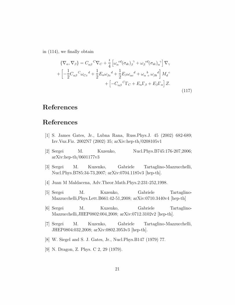
in (114), we finally obtain

{∇α,∇β} = C Cαβ ∇C +

ı

4

[

ω cdα (σdc)

γβ + ω cd

β (σdc)γ

α

]

∇γ

+[

−1

2C C

αβ ω dCc +

1

2Eαω

dβc +

1

2Eβω

dαc + ω b

α c ωd

βb

]

M cd

+[

−C Cαβ ΓC + EαΓβ + EβΓα

]

Z.

(117)

References

References

[1] S. James Gates, Jr., Lubna Rana, Russ.Phys.J. 45 (2002) 682-689;

Izv.Vuz.Fiz. 2002N7 (2002) 35; arXiv:hep-th/0208105v1

[2] Sergei M. Kuzenko, Nucl.Phys.B745:176-207,2006;

arXiv:hep-th/0601177v3

[3] Sergei M. Kuzenko, Gabriele Tartaglino-Mazzucchelli,

Nucl.Phys.B785:34-73,2007; arXiv:0704.1185v3 [hep-th].

[4] Juan M Maldacena, Adv.Theor.Math.Phys.2:231-252,1998.

[5] Sergei M. Kuzenko, Gabriele Tartaglino-

Mazzucchelli,Phys.Lett.B661:42-51,2008; arXiv:0710.3440v4 [hep-th]

[6] Sergei M. Kuzenko, Gabriele Tartaglino-

Mazzucchelli,JHEP0802:004,2008; arXiv:0712.3102v2 [hep-th].

[7] Sergei M. Kuzenko, Gabriele Tartaglino-Mazzucchelli,

JHEP0804:032,2008; arXiv:0802.3953v3 [hep-th].

[8] W. Siegel and S. J. Gates, Jr., Nucl.Phys.B147 (1979) 77.

[9] N. Dragon, Z. Phys. C 2, 29 (1979).

21