A Design of Q -shift Filter for Dual -Tree Complex Wavelet Transforms · A Design of Q -shift Filter for Dual -Tree Complex Wavelet Transforms Faezeh Yeganli Submitted to the Institute

A Design of Q-shift Filter for Dual-Tree Complex

Wavelet Transforms

Faezeh Yeganli

Submitted to the Institute of Graduate Studies and Research

in partial fulfillment of the requirements for the Degree of

Master of Science

in Electrical and Electronic Engineering

Eastern Mediterranean University January 2010

Gazimagusa, North Cyprus

Approval of the Institute of Graduate Studies and Research

Prof. Dr. Elvan Yilmaz Director (a) I certify that this thesis satisfies the requirements as a thesis for the degree of Master of Science in Electrical and Electronic Engineering. Assoc. Prof. Dr. Aykut Hocanin Chair, Department of Electrical Engineering We certify that we have read this thesis and that in our opinion it is fully adequate in scope and quality as a thesis for the degree of Master of Science in Electrical and Electronic Engineering.

Prof. Dr. Runyi Yu Supervisor

Examining Committee

1. Prof. Dr. Huseyin Ozkaramanli

2. Prof. Dr. Runyi Yu

3. Assoc. Prof. Dr. Hasan Demirel

iii

ABSTRACT

In this work a new method of designing filter for Dual-tree complex wavelet

transform is presented. In the new method, the space of orthonormal wavelet filters is

defined in terms of some parameters, these parameters are used to design Q-shift filters

to have desirable properties including good smoothness and support in [-2p/3, 2p/3]. The

constraints in parameterization method lead to wavelets having two vanishing moments.

For obtaining the group delay of 1/4 sample period and minimizing the magnitude or

energy in stop band [2p/3, p], Kingsbury minimized the energy in this domain. In the

proposed method in this work, we minimized the peak magnitude of filters in the stop

band. The design approach is illustrated with four examples. The results are compared

with Kingsbury’s Q-shift in ana lyticity measures, shift-invariance property and half-

sample delay.

The designed filters are then used in image denoising. We used the Bivariate

shrinkage algorithm for wavelet coefficient modeling and thresholding. Three images

(Boat, Baboon, and Cameraman) have been used for test. The experimental results are

compared with those obtained using Kingsbury’s Q-shift filters.

Keywords: Dual-tree complex wavelet transforms, Q-shift filters, Orthogonal wavelets,

Parameterization, Image denoising.

iv

ÖZ

Bu çalismada Ikili agaç kompleksi dalgacik dönüsümü için filtre tasarlamanin

yeni bir yöntemi sunulmaktadir. Yeni yöntemde ortonormal dalgacik filtrelerinin alani

parametrelerle belirlenmektedir, sonra bu parametreler iyi pürüzsüzlük ve [-2p/3,

2p/3]’de destek de dahil istenen özelliklere sahip Q-shift filtrelerinin tasarlanmasinda

kullanilmaktadir. Parametrizasyon yöntemindeki kisitlar dalgaciklarin iki kaybolma

hareketine sahip olmasina neden olmaktadir.

1/4 örnek periyodunun grup gecikmesini elde etmek ve [2p/3, p]’de istenmeyen

büyüklük veya enerjiyi asgariye indirmek için Kingsbury bu alandaki enerjiyi minimize

etmistir. Bu çalismada önerilen yöntemde filtrelerin tepe büyüklügünü söndürme

kusaginda minimize ettik. Sekilli örnekler tasarimin yaklasimini göstermektedir ve

sonuçlar çözümleyicilik ölçümünde ler, shift-degismezlik özelliginde ve yarim örnek

gecikmesinde Kingsbury’nin Q-shift’i ile karsilastirilabilirdir.

Tasarlanan filtreler görüntü gürültüsüzlestirmede kullanilmaktadir. Dalgacik

katsayi modellemesi ve esiklemesi için iki degiskenli fire algoritmasini kullandik. Test

için üç image (Kayik, Babun ve Kameraman) kullanilmistir ve deneysel sonuçlar

Kingsbury'nin Q-shift filtrelerinin kullanilmasiyla elde edilenlerle karsilastirilmistir.

Anahtar sözcükler: Ikili agaç kompleksi dalgacik dönüsümü, Q-shift filtresi, Ortogonal

dalgaciklar, Parametrizasyon, Görüntü gürültüsüzlestirme.

DEDICATION

v

To my beloved Father MirMahmoud and Mother Alvan

and

My sweetie sisters Faegheh, Hanieh, and Sepideh

vi

ACKNOWLEDGMENT

I would like to express my sincere thanks to my supervisor Prof. Dr. Runyi Yu

for his help and guidance. It was a pleasure and honor for me to work with him.

I owe tremendously a lot to my family who allowed me to travel all the way from

Iran to Cyprus and supported me all throughout my studies. I would like to dedicate this

thesis to them as an indication of their significance in my life.

I would like to thank H. M Paiva , Empresa Brasileira de Aeronáutica

(EMBRAER), São José dos Campos, Brazil, for providing the MATLAB code of

parameterization.

Finally, special thanks to my dear friends for their emotional help,

encouragements, and supports.

vii

TABLE OF CONTENTS

ABSTRACT...................................................................................................................... iii

ÖZ ..................................................................................................................................... iv

DEDICATION .................................................................................................................. iv

ACKNOWLEDGMENT................................................................................................... vi

LIST OF TABLES ............................................................................................................ ix

LIST OF FIGURES ........................................................................................................... x

LIST OF SYMBOLS/ABBREVIATIONS ...................................................................... xii

1 INTRODUCTION .......................................................................................................... 1

1.1 Introduction .............................................................................................................. 1

1.2 Organization............................................................................................................. 3

2 DUAL-TREE COMPLEX WAVELET TRANSFORM ................................................ 4

2.1 Introduction .............................................................................................................. 4

2.2 Wavelet Transform .................................................................................................. 4

2.3 Complex Wavelets and DT CWT ............................................................................ 7

2.3.1 The DT CWT .................................................................................................... 8

2.3.2 The Half Sample Delay Condition.................................................................. 10

2.4 Filter Design for the DT CWT ............................................................................... 11

2.4.1 Q-shift Filter Design ....................................................................................... 12

2.5 Two-Dimensional DT CWT .................................................................................. 13

3 Q-SHIFT FILTER DESIGN OF DUAL-TREE FILTER BANKS .............................. 16

3.1 Introduction ............................................................................................................ 16

viii

3.2 Filter Requirements for Q-shift Complex Wavelets .............................................. 17

3.3 A Parameterization of Orthonormal Filters ........................................................... 20

3.4 Q-shift Filter Design Procedure ............................................................................. 23

3.5 Design Examples.................................................................................................... 24

3.6 Mathematical Properties of the Q-shift Filters....................................................... 34

4 IMAGE DENOISING USING Q-Shift FILTERS........................................................ 43

4.1 Introduction ............................................................................................................ 43

4.2 Image Denoising Using the Designed Q-shift Filter.............................................. 43

4.2.1 Bivariate Shrinkage Denoising ....................................................................... 44

4.3 Experimental Results ............................................................................................. 45

5 CONCLUSION AND FUTURE WORK ..................................................................... 51

REFERENCES ................................................................................................................ 54

ix

LIST OF TABLES

Table 3.1: Coefficients of Q-shift filter 0h ...................................................................... 25

Table 3.2: Mathematical properties of designed Q-shift filter......................................... 37

Table 3.3: Mathematical properties of Kingsbury’s Q-shift filter ................................... 37

Table 4.1: Averaged PSNR values (in dB) of denoised images for different noisy images

.......................................................................................................................................... 47

x

LIST OF FIGURES

Figure 2.1: Tree of DWT ................................................................................................... 5

Figure 2.2: Complex wavelets with analyticity property [2] ............................................. 8

Figure 2.3: Analysis filter banks of DT CWT ................................................................... 9

Figure 2.4: Synthesis filter banks of DT CWT .................................................................. 9

Figure 2.5: Wavelet decomposition of an image in one stage [21] ................................. 13

Figure 2.6: The wavelets in space domain (LH, HL, and HH) [21] ................................ 14

Figure 2.7: 2D dual-tree complex wavelets [21] ............................................................. 15

Figure 3.1: Q-shift dual-tree in 3 stages........................................................................... 18

Figure 3.2: Normalized coefficients of 0h (length= 12) .................................................. 26

Figure 3.3: Magnitude and phase response of 0h (length= 12) ....................................... 26

Figure 3.4: Group delay of scaling filter 0h (length=12) ................................................. 27

Figure 3.5: Magnitude spectra of complex wavelets gh jψψ + (length= 12) ................. 27

Figure 3.6: Normalized coefficients of 0h (length= 14) .................................................. 28

Figure 3.7: Magnitude and phase response of 0h (length=14) ........................................ 28

Figure 3.8: Group delay of scaling filter 0h (length= 14) ................................................ 29

Figure 3.9: Magnitude spectra of complex wavelets gh jψψ + (length= 14) ................. 29

Figure 3.10: Normalized coefficients of 0h (length= 16) ................................................ 30

Figure 3.11: Magnitude and phase response of 0h (length= 16) ..................................... 30

Figure 3. 12: Group delay of scaling filter 0h (length= 16) ............................................. 31

xi

Figure 3.13: Magnitude spectra of complex wavelets gh jψψ + (length= 16) ............... 31

Figure 3.14:Normalized coefficients of 0h (length= 18) ................................................. 32

Figure 3.15: Magnitude and phase response of 0h (length= 18) ..................................... 32

Figure 3.16: Group delay of scaling filter 0h (length= 18) .............................................. 33

Figure 3.17: Magnitude spectra of complex wavelets gh jψψ + (length= 18) ............... 33

Figure 3.18: Comparison of Sobolev regularity .............................................................. 38

Figure 3. 19: Comparison of Holder regularity ............................................................... 38

Figure 3.20: Comparison of analyticity measure ( 2I ) ..................................................... 40

Figure 3.21: Comparison of analyticity measure ( ∞I ) .................................................... 40

Figure 3.22: The comparison results of shift invariance measure ( HI 2 ) ......................... 41

Figure 3.23: The comparison results of shift invariance measure ( HI∞ )......................... 41

Figure 3.24: The half-sample delay error ( 2E )................................................................ 42

Figure 3.25: The half-sample delay error ( ∞E ) ............................................................... 42

Figure 4.1: Boat: (a) Original image, (b) Noisy image ( 10=σ , PSNR= 13.6335), (c)

Denoised image by Kingsbury’s Q-shift filter (PSNR= 34.3487), (d) Denoised image by

designed Q-shift filter (PSNR= 33.4932) ........................................................................ 48

Figure 4.2: Baboon (a) Original image, (b) Noisy image ( 15=σ , PSNR= 15.0952), (c)

Denoised image by Kingsbury’s Q-shift filter (PSNR= 27.5924), (d) Denoised image by

designed Q-shift filter (PSNR= 26.6104) ........................................................................ 49

Figure 4.3: Cameraman (a) Original image, (b) Noisy image ( 25=σ , PSNR= 11.6575),

(c) Denoised image by Kingsbury’s Q-shift filter (PSNR= 31.7490), (d) Denoised image

by designed Q-shift filter (PSNR= 29.6833) ................................................................... 50

xii

LIST OF SYMBOLS/ABBREVIATIONS

)(nc Scaling function coefficient

),( njd Wavelet coefficient

2E Energy of half sample delay error

∞E Half-sample delay error

)(0 ng Low pass filter in primal filter bank

)(1 ng High pass filter in dual filter bank

)(0 nh Low pass filter in primal filter banks

)(1 nh High pass filter in dual filter bank

H Hilbert transform

2LH 4L tap low pass filter

2I Analyticity measure

∞I Analyticity measure

HI2 Shift invariance measure of primal filter bank

GI 2 Shift invariance measure of dual filter bank

HI∞ Shift invariance measure of primal filter bank

GI∞ Shift invariance measure of dual filter bank

iχ Variable of parameterization method

xiii

)(tφ Scaling function

)(tψ Wavelet

)(thψ Primal wavelet

)(tgψ Dual wavelet

Bishrinkage Bivariate shrinkage

CQF Conjugate quadrature filter

CWT Complex wavelet transform

DT CWT Dual tree complex wavelet transform

DWT Discrete wavelet transform

PDF Probability distribution function

PSNR The peak signal to noise ratio

Q-shift Quarter shift

1

Chapter 1

1 INTRODUCTION

1.1 Introduction

Dual-Tree Complex Wavelet Transform (DT CWT) is one of a most important

development in signal processing domain. It was first introduced by Kingsbury [1].

Generating complex coefficients by DT CWT introduces limited redundancy and allows

the transform to provide shift invariance and directional selectivity of filters. These

properties make it useful in areas of signal and image processing [2].

By understanding the concept of Hilbert transform pairs, the DT CWT achieves

desirable properties such as nearly shift invariance with limited redundancy. In DT CWT

one wavelet is Hilbert transform of the other and scaling filters in primal filter banks

should be designed to be offset from each other by a half sample delay [1, 3, 4]. This

fundamental concept of Hilbert transform of wavelet bases relates to existence of two

filter banks making together a dual-tree of filter banks. If the Hilbert transform pair

requirement is satisfied, many properties are shared by the primal and the dual filter

bank.

This work is concern with the design of filters for DT CWT structure. There are

two approaches to the design of dual-tree filter banks. The first is designing the primal

and the dual filter banks at the same time. Kingsbury’s Q-shift solution [5] and Selesnick

2

common factor solution [6] fall in this category. The second is design the dual filter

banks from an existing filter banks such as the Daubechies biorthogonal filter bank [5].

The idea of Q-shift filters is presented in the work of Kingsbury in [7, 8] for

improving orthogonality and symmetry properties of filter banks in dual-trees. Then a

new designed has been proposed in [9] for optimizing the Q-shift filters. In a Q-shift

filters a half sample delay is obtained with filter delays of 1/4 or 3/4 of a sample period,

and this is achieved with an asymmetric even length primal filter and its time reverse

[9].

A parameterization of orthonormal wavelets was introduced by Sherlock and

Monro in [10] and recently extended in [11]. The parameterization method enables us to

describe the space of orthonormal wavelets in terms of a set of parameters. The

coefficients for all orthonormal perfect reconstruction FIR filters are generated with a

simple recurrence [10, 11].

In this work, we present a new design technique for Q-shift filters. The new

design method is based on parameterization of orthonormal wave lets with two vanishing

moments. The peak magnitude of the low pass filter in dual-tree structure is minimized

in [2p/3, p] instead of the energy used by Kingsbury. The aim of this work is to design a

Q-shift filter according to parameterization of wavelet filters. The proposed approach

can lead to an FIR filter bank for analytic complex wave lets. In addition, filter bank

properties such as orthogonality, vanishing moments and other properties can be

incorporated in the design procedure.

3

1.2 Organization

The DT CWT is briefly introduced in Chapter 2. Its structure, filter designing

and extension to two dimensional are described in this chapter. In Chapter 3, a Q-shift

filter design is defined and filter requirements for Q-shift filter design are explained.

Then the parameterization method is introduced. We present design examples in this

chapter. After designing, the mathematical properties of designed filter related to its

analyticity and shift invariance are considered and compared with Kingsbury’s Q-shift

filters.

In Chapter 4, we study the application of DT CWT in image denoising. Several

standard images are used to study the denoising problem. Each image is corrupted by an

additive white Gaussian noise at various levels and then denoised by using a DT CWT.

The denoising method is used for three images (Boat, Baboon and Cameraman). The

results of denoising are illustrated in this chapter.

Chapter 5 summarized the material presented in this work. It also discusses the

possible future work.

4

Chapter 2

2 DUAL-TREE COMPLEX WAVELET TRANSFORM

2.1 Introduction

A Dual-Tree Complex wavelet Transform (DT CWT) is a recently development

in wavelet domain that was first produced by Kingsbury in [1]. Its structure with good

properties likes shift-invariance and good directionality in two and higher dimensions

make it useful in signal and image processing applications. It achieves this with a limited

redundancy (redundancy factor of D2 for D dimensional signals).

In this chapter we will introduce DT CWT. At first we briefly explain wavelet

domain analysis, and then Discrete Wave let Transform (DWT) and its properties. Then

DT CWT and its characterization are introduced and filter designed procedure for DT

CWT is explained. Finally we explain extension of the DT CWT to two dimensional

(2D).

2.2 Wavelet Transform

Wavelets are famous domain in signal processing. They are stretched and shifted

version of real valued band pass wavelets )(tψ . Their combination with low pass scaling

function )(tφ can form an orthonormal basis expansion that provides a time-frequency

5

analysis of signal. We can express any signal )(tx in terms of wavelets and scaling

function as in (2.1) [2]:

)2(2),()()()(0

2 ntnjdntnctx j

n j n

j

−+−= ∑ ∑ ∑∞

−∞=

∞

=

∞

−∞=

ψφ (2.1)

where )(nc is the scaling function coefficient, and ),( njd is the wavelet coefficient that

are computed respectively:

∫∞

∞−−= dtnttxnc )()()( φ (2.2)

∫∞

∞−−= )2()(2),( 2 nttxnjd j

jψ . (2.3)

Time-frequency analysis is controlled by scale factor j and time factor n.

There are algorithms to compute a scaling function and wavelet based on

weighted sum of shifted scaling function (basis) that produce a discrete-time low pass

filter )(0 nh and high pass filter )(1 nh , and upsampling and downsampling operations

which make filter banks structure. The DWT consists of recursively applying two-

channel filter bank shown in Figure 2.1. We refer to [2, 12] on theory about wavelet

domain analysis.

2↓

2↓

2↓

2↓

2↓

2↓

x

1Level2Level

3Level

Figure 2.1: Tree of DWT

6

Filters )(0 nh , )(1 nh makes a convenient parameterization for designing wavelets

and scaling functions with properties like compact support, orthogonality to lower order

polynomials (vanishing moments). These properties make wavelets more useful than

Fourier analysis, and enable to represent many types of signals which are not matched

by the Fourier basis [2].

The DWT have these properties: good compression of signal energy, perfect

reconstruction with short support filters, no redundancy and very low computation. In

spite of good properties with real wavelets, there are some fundamental problems [4]:

1) Oscillations: Wavelets are band pass functions, so their coefficients oscillate

positive and negative around singularities (jump and spikes); this makes wavelet

based processing to have some complexities.

2) Shift variance: The wavelet coefficients will oscillate around singularities by a

small shift of signal, though it complicates wavelet domain processing.

3) Aliasing: Computing wavelet coefficients by discrete time upsampling and down

sampling operations makes aliasing.

4) Lack of directionality: Multi dimensional wavelet coefficients produce a pattern

that is simultaneously oriented in several directions. This lack of directional

selectivity makes problems in image processing.

Complex wavelets provide solution to these shortcomings [2].

7

2.3 Complex Wavelets and DT CWT

The DWT’s problems [2] solved by Fourier transform’s properties. Unlike the DWT,

Fourier transform doesn’t suffer from mentioned problems. The Fourier transform

analysis is based on complex complex-valued oscillating sinusoids:

)sin()cos( tjte tj Ω+Ω=Ω . (2.4)

The oscillating real part (cosine) and imaginary part (sine) components form a

Hilbert transform pair that produce an analytic signal tje Ω which is supported on only

half of the frequency axis ( 0>Ω ).

Imitating the above representation, we can get a Complex wavelet transform (CWT)

with complex valued scaling function [2]:

)()()( tjtt irC ψψψ += . (2.5)

A complex valued wavelet coefficient is defined as below:

),(),(),( njjdnjdnjd irC += . (2.6)

According to (2.4) and (2.5), )(trψ is real and even and )(tiψ is imaginary and

odd and by forming the Hilbert transform pair they make )(tCψ to be analytic signal

[2]. These properties are illustrated in Figure 2.2.

The design of CWT makes some new problems that DWT doesn’t have , so new

approach is needed.

8

Figure 2.2: Complex wavelets with analyticity property [2]

2.3.1 The DT CWT

For implementing an analytic wavelet transform, Kingsbury introduced a DT

CWT structure in [1]. The DT CWT employs two real DWT in its structure. The first

DWT gives the real part of the transform and second part gives the imaginary part. The

analysis and synthesis Filter banks used in DT CWT are shown in Figures 2.3 and 2.4

respectively.

The two real wavelet transforms use two different set of filters that satisfying the

perfect reconstruction condition. Filters )(0 nh , )(1 nh and )(0 ng , )(1 ng denote the low

pass/high pass filter pairs for the upper and lower filter banks respectively. Both filters

are real but their combination produce a complex wavelet. For satisfying a perfect

reconstruction condition the filters are designed to make a complex wavelet

)()()( tjtt gh ψψψ += approximately analytic by two real wavelet transforms

)(thψ and )(tgψ . Equivalently they are designed so that the lower wavelet )(tgψ is the

Hilbert transform of upper wavelets )(thψ ; )()( tt hg ψψ Η≈ [2, 3, 6].

9

*

*

+

+

*

*

+

*

*

2↓

2↓

2↓

2↓

2↓

2↓

2↓

2↓

2↓

2↓

2↓

2↓

x

1Level2Level

3Level

+

+

+

Figure 2.3: Analysis filter banks of DT CWT

0~H

1~H

1~G

2↑

2↑0

~H

1~H

2↑

2↑

2↑

00

~H

01

~H2↑

2↑

2↑

2↑ 2↑

2↑

2↑

2↑

2↑

0~G

01

~G

1~

G

0~G

00

~G

Figure 2.4: Synthesis filter banks of DT CWT

In the inverse of DT CWT, like the forward transform, the real part and

imaginary part are each inverted and the inverse of the two real DWTs gives a two real

signal and finally the average of two real signals gives a final output. We can get an

original signal from either real part or imaginary part alone.

10

2.3.2 The Half Sample Delay Condition

Several analysis are made about the fact that one wavelet is approximately the

Hilbert transform of the other. If we want wavelets form a Hilbert transform pair, we

need to design low pass filters satisfying this property. Now let

∑=n

hh tnht )()(2)( 1 φψ (2.7)

∑=n

hh tnht )()(2)( 0 φφ (2.8)

where )()1()( 01 ndhnh n −−= ; for lower filter bank )(tgψ , )(tgφ and )(1 ng are defined

similarly. Assuming that both real wavelets are orthonormal, from [2, 3] these filters

should satisfy the property as below:

)5.0()( 00 −≈ nhng . (2.9)

It means that one of them should be approximately half sample shift of the other.

The Fourier transform of (2.9) and its magnitude and phase are

)()( 05.0

0jwwjjw eHeeG −= (2.10)

)()( 00jwjw eHeG = (2.11)

weHeG jwjw 5.0)()( 00 −∠=∠ . (2.12)

By having this property, wavelets will form Hilbert transform pair

( )()( tt hg ψψ Η≈ ) and the complex wavelet )()( tjt gh ψψ + will be approximately

analytic, and the DT DWT is nearly shift-invariant. Also when the complex wavelets are

analytic, the two filter banks share common properties including orthogonality (or

biorthogonality) [13, 14].

11

Now we understand the aim of the Hilbert transform of wavelet bases. This

fundamental concept relates to the existence of two filter banks making together a dual-

tree of filter banks.

2.4 Filter Design for the DT CWT

As mentioned in the previous sections, filter properties in the filter banks

structure play a significant role in obtaining the important properties of wavelet domain.

So designing filters that satisfy these properties is important.

Several methods proposed for designing filters for the DT CWT structure. In

these methods the designed filters have some desired properties like: approximately half-

sample delay property, perfect reconstruction, finite support filters (FIR filters),

vanishing moments, linear phase filters.

The early methods for designing filters include linear-phase biorthogonal

solution, Q-shift solution, and common factor solution. The first method is introduced in

[1, 16]; common factor solution is explained in [6]; and Q-shift method that we used for

designing a filter in this thesis is introduced by Kingsbury in [7]; and will be explained

in next section. See [2] and [13] for more about the design of DT filter banks.

The other important thing in filter designing for dual-trees is that the first stage

of the dual-tree filter banks should be different from the other stages. The half sample

delay condition shouldn’t be used for the first stage. For the first stage, it is necessary

only to translate one set of filters by one sample to the other ( )1()( 00 −= nhng ) and any

set of perfect reconstruction filter can be used for first stage. For more explanation and

its proof we refer to [2].

12

2.4.1 Q-shift Filter Design

This method was introduced by Kingsbury in [7]. Satisfying linear-phase

property of )(0 nh is achieved by

)1()( 00 nNhng −−= . (2.13)

where N (even) is the length of )(0 nh which is supported in 10 −≤≤ Nn . In this case

the magnitude part of (1.12) is satisfied but the phase part (2.12) is not and will be like

below [2]:

)()( 00jwjw eHeG = (2.14)

weHeG jwjw 5.0)()( 00 −∠≠∠ . (2.15)

The quarter-shift solved (2.15) problem. From (2.13) we can write

wNjjwjw eeHeG )1(00 )()( −−= . (2.16)

And its phase becomes

wNeHeG jwjw )1()()( 00 −−−∠=∠ . (2.17)

From (2.12) we can rewrite (2.17) like below:

wNeHweH jwjw )1()(5.0)( 00 −−−∠≈−∠ . (2.18)

Then we can obtain below formula:

wwNeH jw 25.0)1(5.0)(0 +−−≈∠ . (2.19)

So, )(0 nh is approximately linear-phase and symmetric around 25.0)1(5.0 −−= Nn ; that

is a quarter away from a natural point of symmetry. So this method is named Q-shift

method. In Q-shift method the imaginary part of the complex wavelet is a time-reversed

of real part ( )1()( tNt hg −−= ψψ ) [2, 7].

13

Therefore Q-shift method is to design filters satisfying perfect reconstruction

condition and approximately linear-phase condition with group delay required to be a

quarter.

2.5 Two-Dimensional DT CWT

One of the advantages of DT CWT is that it can be used to implement two-

Dimensional (2D). In 2D, DT CWT saved desirable properties of 1D case and has

effective properties like directional selectivity. In particular, 2-D dual-tree wavelets are

not only approximately analytic but also oriented and thus natural for analyzing and

processing oriented singularities like edges in images [2].

At first we explains 2D DWT and then discuss 2D DT CWT. Using the wavelet

transform for image processing requires implementation of a 2D version of analysis and

synthesis filter banks. In this case, first, 1D analysis filter banks is applied to the

columns of the image and then applied to the rows. Therefore four sub-band images (LL,

LH, HL, HH) are obtained; see Figure 2.5. For obtaining original image, the 2D

synthesis filter bank combines the four sub-band image [2].

Figure 2.5: Wavelet decomposition of an image in one stage [21]

14

The separable (row-column) implementation of the 2D DWT is characterized by

three wavelets as below [2]:

)()(),(1 yxyx ψφψ = (LH wavelet)

)()(),(2 yxyx φψψ = (HL wavelet)

)()(),(3 yxyx ψψψ = (HH wavelet).

The LH (Low-High) and HL wavelets are or iented vertically and horizontally,

the HH wavelets mix two diagonal orientations ( o45+ and o45− ). Figure 2.6 illustrates

these wavelets [21].

Figure 2.6: The wavelets in space domain (LH, HL, and HH) [21]

The separable DWT is unable to isolate these orientations. 2D DT CWT produce

oriented wavelets that are oriented in six distinct directions. In each direction, one of the

two wavelets can be interpreted as the real part while the other wavelet can be

interpreted as the imaginary part of the complex-valued 2D wavelet. The complex 2D

DT operating as four critically sampled separable 2D DWTs operating in parallel. The

Figure 2.7 illustrates 2D DT CWT.

We can see in Figure 2.7, the wavelets are or iented in the same six directions but

there are two in each direction. The six wavelets on the first are interpreted as a real part

15

and the six wavelets on the second row are imaginary part of a set of six complex

wavelets. The third row is the magnitude of the six complex wavelets [21].

Figure 2.7: 2D dual-tree complex wavelets [21]

While the wavelets are oriented, approximately analytic, and non-separable, the

implementation is very efficient and makes it useful in many applications of image

processing such as denoising.

16

Chapter 3

3 Q-SHIFT FILTER DESIGN OF DUAL-TREE FILTER

BANKS

3.1 Introduction

We have described the DT CWT. This introduces limit redundancy and allows

the transform to provide approximate shift invariance and directionality selection of

filters while preserving the usual properties of perfect reconstruction and computational

efficiency responses. We analyze the new designed filters in terms of directionality and

shift invariance.

In this chapter we present a new design of Q-shift filters for DT CWT. The idea

of using Q-shift approach is motivated by the work of Kingsbury in [7] for improving

orthogonality and symmetry properties of filter banks. Q-shift form employs a single

design of even-length filter with asymmetric coefficients. The DT CWT structure

requires most of the wavelet filters to have a well controlled group delay [7, 9]

(equivalent to quarter of a sample period) to achieve approximately shift invariance.

In Q-shift filters a half-sample delay difference is obtained with filter delays of

1/4 and 3/4 of a sample period and this is achieved with an asymmetric even-length filter

)(0 zH and its time reverse. Also lower tree filters are time-reverse of upper tree filters

and reconstruction filters are the time-reverse of analysis filters, this make transform use

17

shorter filters and all filters form orthonormal set (bases are orthonormal) beyond level

one. Then the two trees are matched very well and have a more symmetric sub-sampling

structure [7, 15].

In this work we use parameterization method of orthogonal wavelet filter banks.

This method was first introduced by Sherlock and Monro in [10] and then extended in

[11]. According to the mentioned method, the space of orthonormal wavelet is described

by a set of parameters [10]. The parameterization is not unique for different roots of the

polynomial may be chosen. The advantage of this method is that it is able to

parameterize wavelets that have vanishing moments greater than one, in this work is

equal to two [11].

As we know one of the most important properties of complex wavelet filters in

dual-tree filter banks is their analyticity. Other important mathematical properties of

complex wavelet filters are consequences of analyticity.

In Section 3.2, the requirements of Q-shift filter design will explain. In Section

3.3 the parameterization method will introduced. The design procedure is given in

Section 3.4; Section 3.5 presents some design examples. The mathematical properties of

complex wavelet filters introduced and their comparison between designed Q-shift filter

and Kingsbury’s Q-shift filter are shown in Section 3.6.

3.2 Filter Requirements for Q-shift Complex Wavelets

Consider the Q-shift dual-tree in Figure 3.1 in which all filters beyond level 1 are

even-length.

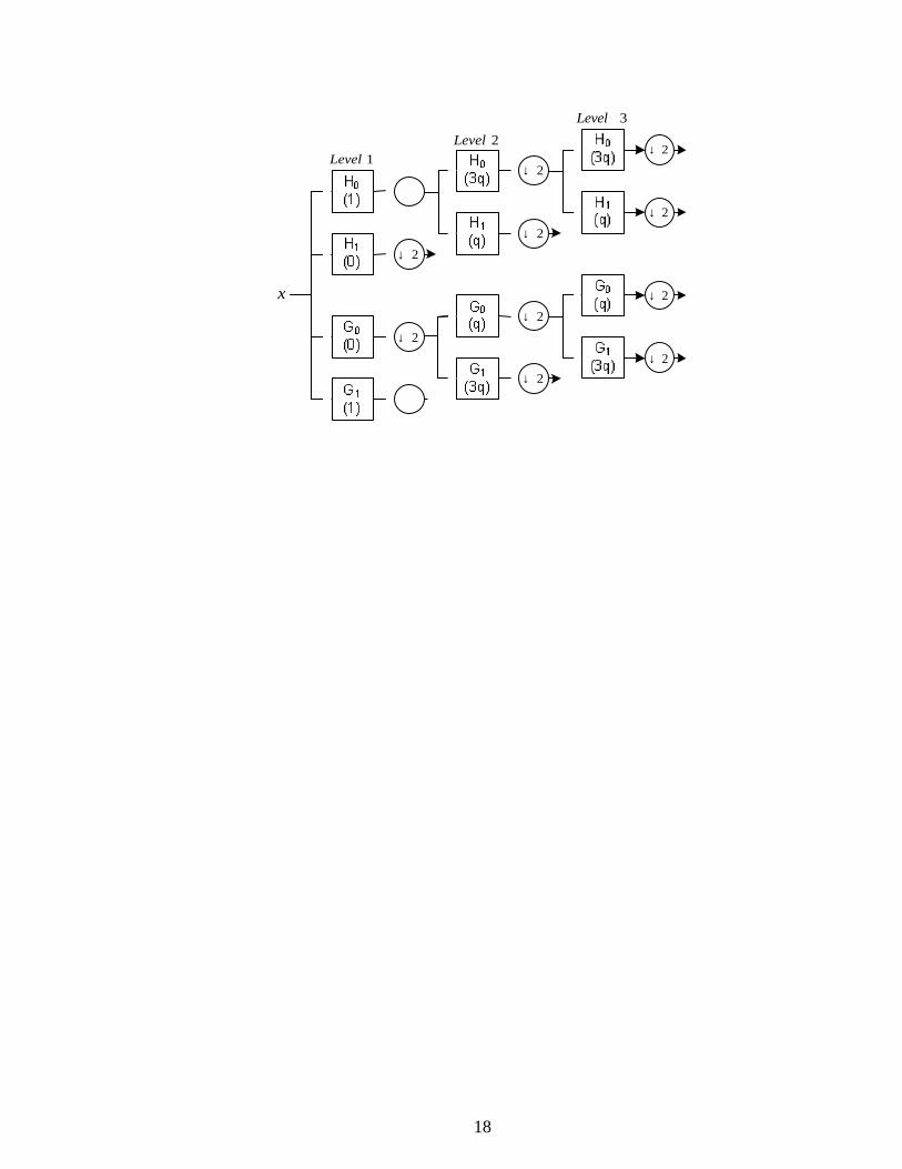
18

2↓

2↓

2↓

2↓

2↓

2↓

2↓

2↓

2↓

2↓

2↓

2↓

x

1Level2Level

3Level

Figure 3.1: Q-shift dual-tree in 3 stages

Our aim is to design the Q-shift filter 0H with desirable properties. In this method of

designing, we the properties of Kingsbury’s Q-shift design [9] are complemented by

parameterization method. The key properties of Q-shift filters according to [9] are:

1) No aliasing: The symmetry properties of the Q-shift filters can be obtained by

setting up these equations between the filters of dual-tree filter banks [9]

)()(~01 zzHzH −= (3.1)

)(~

)( 01

1 zHzzH −= − . (3.2)

2) Perfect Reconstruction: By satisfying the standard condition of perfect

reconstruction of filter banks we obtain his property [9, 15]. So we will have

2)(~)()(~)( 0000 =−−+ zHzHzHzH . (3.3)

3) Orthgonality: The dual filter bank can achieve the orthogonality of primal filter

bank if the half-sample delay condition is met [16]. In the Q-shift filters, the

lower filter is the time reverse of upper filter and for satisfying orthogonality we

should setting up this equation

19

)()( 100

−= zHzG . (3.4)

4) Group Delay ≈ 1/4 sample for 0H and 3/4 for 0G : To get this property we use

Kingsbury’s method in [7, 9]. To obtain 2L-tap low pass filters, 0H and 0G with

1/4 and 3/4 sample delays, a 4L-tap linear phase and symmetric low pass filter

)(2 zH L with a delay of 1/2 sample is designed as follows

)()()( 20

1202

−−+= zHzzHzH L . (3.5)

So the subsample filter 0H will have a half of delay of )(2 zH L (1/4 sample).

5) Good smoothness when iterated over scale.

6) Finite support in (-2p/3, 2p/3), that is, 0)(0 ≈jweH For w∉[-2p/3, 2p/3].

To achieve the fifth and sixth properties we come back to one of the important

properties of discrete-time systems that are shift invariant. We say, a discrete-

time system is µ-shift-invariant if a shift in input results the output shifted as well

[16]. And the M-fold decimator (down sampler) is µ-shift-invariant for input if

its frequency supports in not more than 2p/M and the output shouldn’t have the

aliasing term in same frequency band with length of π2 . As we know one of the

most important properties of DT CWT structures is its shift invariance property

and for achieving this property the conjugate quadrature filters (CQF) should

have support limited in [-2p/3, 2p/3], in addition to the well known half sample

delay condition at high levels and the one sample delay condition in first level

[16].

Analyticity of the complex wavelet filters alone is not enough for the µ-shift-

invariant of DT CWT. We should know that the stop band of )(0 zH at each

20

scale suppresses energy at frequencies where unwanted pass bands appear from

sub sampled filters operating at coarser scales [9, 16]. So we should minimize the

magnitude spectrum or energy in [2p/3, p]. This cut off frequency has been used

by Kingsbury for designing his Q-shift filter. This analysis of µ-shift-invariant

helps explain the success of Q-shift filters in DT CWT based applications.

In this work for obtaining the group delay of 1/4 sample period and minimizing

the magnitude of the )(0 zH in the mentioned method we use )(2 zH L as in [7, 9] and

minimize the maximal magnitude of )(2 zH L instead of the energy used in Kingsbury’s

design in its stop band of [p/3, p].

Minimizing the magnitude of )(2 zH L in the mentioned domain and finally obtain

the Q-shift filter are explained in next section.

7) Vanishing moments: Vanishing moments are feature of wavelets. They are the

number of zeros of scaling filter at 1−=z . Having P vanishing moments means

that wavelets coefficients for Pth order polynomial will be zero. That is any

polynomial signal up to P-1 can be represented completely in scaling space.

More vanishing moments means that scaling function can represent more

complex signals accurately. In this work our design procedure let us to have two

vanishing moments.

3.3 A Parameterization of Orthonormal Filters

The parameterization of the space of two-channel orthonormal FIR filters enable

us to describe the generation of all filters by using a simple recurrence. The method used

here for wavelets has guaranteed the resulting wavelets have two vanishing moments.

21

The remaining degrees of freedom are re-parameterized which lead to a convex set of

feasible parameter values [11].

Let )(0 zH be 2L (= N) length low pass filter, Sherlock and Monro’s recursive

formulas for a filter of length 2(L+1) according to terms of 2L length filter, expressing

the coefficients as in [11]

=

=

)sin(

)cos(

1)1(

1

1)1(

0

α

α

h

h (3.6)

−=

−=−=

=

−++

−+++

++

)(121

)1(2

)(121

)(21

)1(2

)(01

)1(0

)sin(

1,...,2,1,)sin()cos(

)cos(

LLL

LL

LiL

LiL

Li

LL

L

hh

LiLhh

hh

α

αα

α

(3.7)

=

−=+=

=

−+++

−+++

+

++

.)cos(

1,...,2,1,)cos()sin(

)sin(

)(121

)1(12

)(121

)(21

)1(12

)(01

)1(1

LLL

LL

LiL

LiL

Li

LL

L

hh

Lihhh

hh

α

αα

α

(3.8)

As we see that the orthonormal wavelet filters can be completely parameterized

by L angles iα , Li ≤≤1 , which can assume any value in the set of real numbers and any

choice of iα will lead to a valid orthonormal FIR filter banks system, and any system

can be expressed in terms of some choice of iα [10, 11].

For a first vanishing moment the following condition should be satisfied

0)( 10 =−=zzH . (3.9)

From (3.7) -(3.9) we can write )()(0 zH L with angles iα as below

∑∑==

−= −=L

ii

L

iiz

LH11

1)(

0 sincos αα . (3.10)

22

So the first vanishing moment condition will become:

∑−

=

−=1

14

L

iiL α

πα . (3.11)

For second vanishing moment it is necessary to impose this condition:

0)(

1

)(0 =−=z

L

dzzdH

. (3.12)

And finally by doing some mathematical expressions on (3.12) and using above

formulas the second vanishing moment condition will be obtained (The expression and

proof are in [11]):

∑∑ ∑−

=

−

= =− −

−−=2

1

2

1 11 ]2[sin

21

arcsin21 L

kk

L

k

k

iiL ααα . (3.13)

Vanishing moments conditions reduces the number of free parameters to L-1 and

L-2 respectively. For defining a convex region of parameters in 2−LR a new parameter

χ is proposed [11]. Second vanishing moment condition (formula (3.13)) have a real-

valued solution, if and only if the angles iα , 21 −≤≤ Li , satisfy the following

constraints:

21

)2(sin23 2

1 1

≤≤− ∑ ∑−

= =

L

k

k

iiα . (3.14)

But these constraints don’t define a convex region in 2−LR , so for having a convex region

χ is defined as:

∑=

=k

kik

1

2sin αχ , 21 −≤≤ Lk . (3.15)

The constraints can be rewritten as:

21

23 2

1

≤≤− ∑−

=

L

kkχ (3.16)

23

1,...,,1 221 ≤≤− −Lχχχ . (3.17)

And the values of iα , 21 −≤≤ Li are obtained by using the following equations:

)arcsin(21

11 χα = (3.18)

∑−

=

−=1

1

2)arcsin(21 i

kkii αχα . (3.19)

Finally the filter banks coefficients are calculated by (3.6)-(3.8).

By using this method of parameterization in our work we can design Q-shift filer

with mentioned properties. The design procedure is explained in next section.

3.4 Q-shift Filter Design Procedure

Following discussions in Sections 3.2 and 3.3, we now give a design procedure

for Q-shift filter. By knowing the properties of filter; the design procedure starts with

specifying the value of iχ . Parameter iχ is very important parameter in our designing

and produces a convex region for our parameterization. After parameterization, the

magnitude of obtained filter according to the parameters is minimized and finally the

favorite filter will be obtained by recurrence formula. In the following we explain the

design procedure step by step.

Step 0. Specify the basic properties of filter like length of scaling filter.

Step 1. Initialize the value of iχ , then generate the iα by using (3.18) and (3.19).

Step 2. Obtain 0h from iα . At first get Lα from (3.11) and (3.13), then 0h is obtained

from (3-6)-(3.8).

Step 3. Define the 2LH as in (3.5). Then define the magnitude of )(2 zH L in [p/3, p]. This

is for obtaining 0H and 0G with 1/4 and 3/4 sample period respectively.

24

Step 4. Minimize the peak magnitude of )(2 zH L . This is for achieving properties 6 and

7 (Section 3.2) to obtain optimal magnitude.

For minimizing the magnitude of 2LH we use constrained minimization method

by employing ’’fmincon’’ in the optimization toolbox of MATLAB. This function can

find a constrained minimum of a function with several variables. Our variable here is χ

and according to the constraints that we defined for χ to obtaining the convex region of

parameterization, it can start to minimize the magnitude of 2LH .

Step 5. Obtain the low pass filter 0h using ?. Then obtain 0g from 0h , according to

relationship of dual-tree filters in Q-shift filter ( )()( 100

−= zHzG ).

The procedure can be repeated with obtained ? as initial value in Step 1. After

designing the filters, the complex wavelet gh jψψ + is expected to be approximately

analytic.

3.5 Design Examples

We present four examples in this section to illustrate the design approach and its

results. Design examples give filters of length 12, 14, 16, and 18 respectively. The

normalized coefficients of 0h for the mentioned lengths are shown in table 3.1. As we

mentioned in previous section we can easily get the 0g (dual filter bank) by flipping 0h .

25

Table 3.1: Coefficients of Q-shift filter 0h N= 12 N= 14 N= 16 N= 18

0.00017654 0.00202905 0.01944400 -0.05470174 -0.02152764 0.40680833 0.55064137 0.15754572 -0.05006905 -0.01156524 0.00133476 -0.00011613

-0.00754976 -0.00440359 0.00135387 0.00796048 -0.08771886 0.03250019 0.42397196 0.50635403 0.19977468 -0.10585055 -0.02542829 0.05588967 -0.00440359 0.00754976

-0.00246667 -0.00070423 0.01485766 0.00489657 0.03152301 -0.07051195 -0.03670630 0.42121140 0.52959241 0.17913806 -0.04230220 -0.01602463 0.00589103 -0.01936757 -0.00038895 0.00136235

0.00000682 0.00003496 0.00006221 0.00343113 -0.01604502 0.01037313 -0.04315593 -0.02872404 0.40720354 0.55129394 0.15565237 -0.05172803 -0.00687361 0.01534684 0.00311584 -0.00002133 0.00003377 -0.00000659

Figures 3.2, 3.6, 3.10 and 3.14 show the normalized coefficients of 0h . For

different lengths the magnitude and phase response of 0h are illustrated in Figures 3.3,

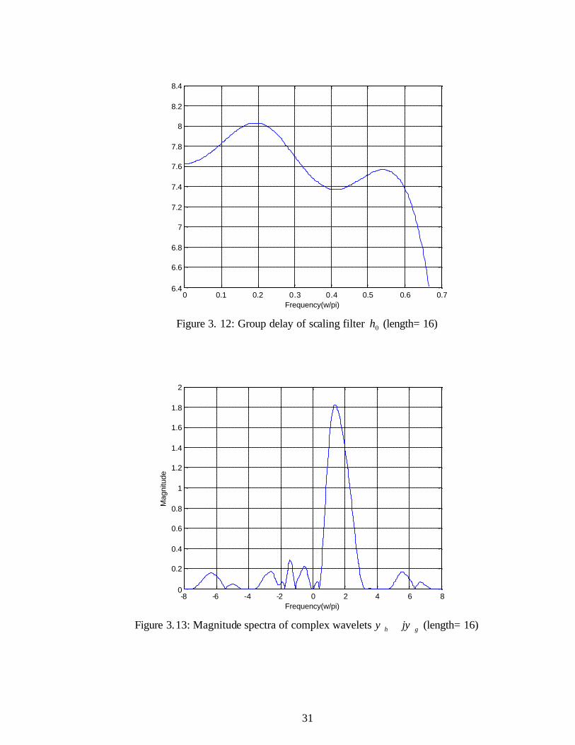
3.7, 3.11, and 3.15. The group delay of 0h are shown in Figures 3.4, 3.8, 3.12, and 3.16.

Finally the analytic wavelet gh jψψ + for mentioned lengths are depicted in Figures 3.5,

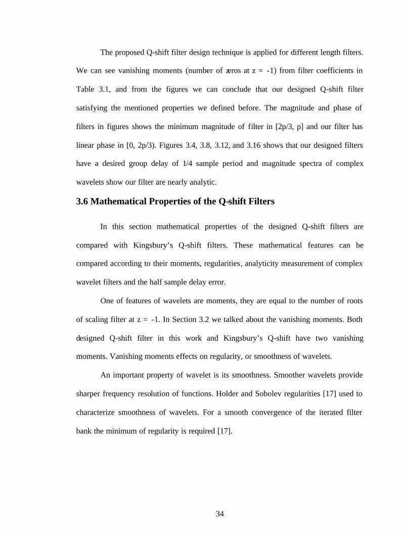
3.9, 3.13, and 3.17.

26

-8 -6 -4 -2 0 2 4 6 8-0.2

-0.1

0

0.1

0.2

0.3

0.4

0.5

0.6

0.7

0.8

Figure 3.2: Normalized coefficients of 0h (length= 12)

0 0.1 0.2 0.3 0.4 0.5 0.6 0.7 0.8 0.9 1-1000

-500

0

Normalized Frequency (×π rad/sample)

Pha

se (

degr

ees)

0 0.1 0.2 0.3 0.4 0.5 0.6 0.7 0.8 0.9 1-150

-100

-50

0

Normalized Frequency (×π rad/sample)

Mag

nitu

de (

dB)

Figure 3.3: Magnitude and phase response of 0h (length= 12)

27

0 0.1 0.2 0.3 0.4 0.5 0.6 0.7

5.35

5.4

5.45

5.5

5.55

5.6

5.65

5.7

5.75

5.8

5.85

Frequency(w/pi)

Figure 3.4: Group delay of scaling filter 0h (length=12)

-8 -6 -4 -2 0 2 4 6 80

0.2

0.4

0.6

0.8

1

1.2

1.4

1.6

1.8

2

Frequency(w/pi)

Mag

nitu

de

Figure 3.5: Magnitude spectra of complex wavelets gh jψψ + (length= 12)

28

-8 -6 -4 -2 0 2 4 6 8-0.2

-0.1

0

0.1

0.2

0.3

0.4

0.5

0.6

0.7

0.8

Figure 3.6: Normalized coefficients of 0h (length= 14)

0 0.1 0.2 0.3 0.4 0.5 0.6 0.7 0.8 0.9 1-1500

-1000

-500

0

Normalized Frequency (×π rad/sample)

Pha

se (

degr

ees)

0 0.1 0.2 0.3 0.4 0.5 0.6 0.7 0.8 0.9 1-100

-50

0

Normalized Frequency (×π rad/sample)

Mag

nitu

de (

dB)

Figure 3.7: Magnitude and phase response of 0h (length=14)

29

0 0.1 0.2 0.3 0.4 0.5 0.6 0.76

6.5

7

7.5

8

8.5

9

9.5

Frequency(w/pi)

Figure 3.8: Group delay of scaling filter 0h (length= 14)

-8 -6 -4 -2 0 2 4 6 80

0.2

0.4

0.6

0.8

1

1.2

1.4

1.6

1.8

2

Frequency (w/pi)

Mag

nitu

de

Figure 3.9: Magnitude spectra of complex wavelets gh jψψ + (length= 14)

30

-8 -6 -4 -2 0 2 4 6 8-0.2

-0.1

0

0.1

0.2

0.3

0.4

0.5

0.6

0.7

0.8

Figure 3.10: Normalized coefficients of 0h (length= 16)

0 0.1 0.2 0.3 0.4 0.5 0.6 0.7 0.8 0.9 1-1500

-1000

-500

0

Normalized Frequency (×π rad/sample)

Pha

se (d

egre

es)

0 0.1 0.2 0.3 0.4 0.5 0.6 0.7 0.8 0.9 1-100

-50

0

Normalized Frequency (×π rad/sample)

Mag

nitu

de (d

B)

Figure 3.11: Magnitude and phase response of 0h (length= 16)

31

0 0.1 0.2 0.3 0.4 0.5 0.6 0.76.4

6.6

6.8

7

7.2

7.4

7.6

7.8

8

8.2

8.4

Frequency(w/pi)

Figure 3. 12: Group delay of scaling filter 0h (length= 16)

-8 -6 -4 -2 0 2 4 6 80

0.2

0.4

0.6

0.8

1

1.2

1.4

1.6

1.8

2

Frequency(w/pi)

Mag

nitu

de

Figure 3.13: Magnitude spectra of complex wavelets gh jψψ + (length= 16)

32

-10 -8 -6 -4 -2 0 2 4 6 8 10-0.2

-0.1

0

0.1

0.2

0.3

0.4

0.5

0.6

0.7

0.8

Figure 3.14:Normalized coeffic ients of 0h (length= 18)

0 0.1 0.2 0.3 0.4 0.5 0.6 0.7 0.8 0.9 1-1500

-1000

-500

0

Normalized Frequency (×π rad/sample)

Pha

se (

degr

ees)

0 0.1 0.2 0.3 0.4 0.5 0.6 0.7 0.8 0.9 1-150

-100

-50

0

Normalized Frequency (×π rad/sample)

Mag

nitu

de (

dB)

Figure 3.15: Magnitude and phase response of 0h (length= 18)

33

0 0.1 0.2 0.3 0.4 0.5 0.6 0.77.8

8

8.2

8.4

8.6

8.8

9

Frequency(w/pi)

Figure 3.16: Group delay of scaling filter 0h (length= 18)

-8 -6 -4 -2 0 2 4 6 80

0.2

0.4

0.6

0.8

1

1.2

1.4

1.6

1.8

Frequency(w/pi)

Mag

nitu

de

Figure 3.17: Magnitude spectra of complex wavelets gh jψψ + (length= 18)

34

The proposed Q-shift filter design technique is applied for different length filters.

We can see vanishing moments (number of zeros at z = -1) from filter coefficients in

Table 3.1, and from the figures we can conclude that our designed Q-shift filter

satisfying the mentioned properties we defined before. The magnitude and phase of

filters in figures shows the minimum magnitude of filter in [2p/3, p] and our filter has

linear phase in [0, 2p/3). Figures 3.4, 3.8, 3.12, and 3.16 shows that our designed filters

have a desired group delay of 1/4 sample period and magnitude spectra of complex

wavelets show our filter are nearly analytic.

3.6 Mathematical Properties of the Q-shift Filters

In this section mathematical properties of the designed Q-shift filters are

compared with Kingsbury’s Q-shift filters. These mathematical features can be

compared according to their moments, regularities, analyticity measurement of complex

wavelet filters and the half sample delay error.

One of features of wavelets are moments, they are equal to the number of roots

of scaling filter at z = -1. In Section 3.2 we talked about the vanishing moments. Both

designed Q-shift filter in this work and Kingsbury’s Q-shift have two vanishing

moments. Vanishing moments effects on regularity, or smoothness of wavelets.

An important property of wavelet is its smoothness. Smoother wavelets provide

sharper frequency resolution of functions. Holder and Sobolev regularities [17] used to

characterize smoothness of wavelets. For a smooth convergence of the iterated filter

bank the minimum of regularity is required [17].

35

By knowing the concept of complex wavelet filters in DT CWT, and according

to Figure 3.1, we define complex wavelet filter as:

)()()( 00 jwjGjwHjwP += (3. 20)

As we mentioned in Section 2.3.2, the complex wavelet is analytic if and only if

CQFs satisfy the one sample delay in first level and the half sample delay condition in

next levels [16]. This property makes wavelets form Hilbert transform pairs and the DT

CWT become nearly shift invariant.

All these condition are gathered in Theorem 4 of [16] that indicates the DT CWT

is µ-shift-invariant at levels more than one if and only if the CQFs satisfy the one sample

delay condition in the first level and half sample delay condition in high levels, and

CQFs are supported in [-2p/3, 2p/3]. The cut off frequency 2p/3 is used in designing

filter for DT CWT in this work and Kingsbury’s work in [9]. The support of CQFs in

DT CWT is in [0, p). For the µ-shift-invariant system the magnitude spectrum (energy)

of its output is insensitive to input shift, and the phase changes linearly [16]. So the

energy is used to calculate the errors in sequel.

By measuring the following errors we want to know that how much our complex

wavelet filter is analytic or how much the CQFs are shift invariance. The half sample

delay errors show how the CQFs could make a half sample delay related to the

analyticity of the complex wavelets. Smaller errors indicate better designed filters.

36

The analyticity measure of complex wavelet filter is obtained by

∫

∫

−

= π

π

π

dwjwP

dwjwPI

2

0

2

2

)(

)( (3.21)

and

)(max

)(max

),[

),0[

jwP

jwPI

w

w

ππ

π

−∈

∈∞ = . (3.22)

For the CQFs, the shift invariance measure can be obtained from HI 2 and GI 2

∫

∫= π

π

π

0

20

32

20

2

)(

)(

dwjwH

dwjwH

I H (3.23)

and

∫

∫= π

π

π

0

20

32

20

2

)(

)(

dwjwG

dwjwG

I G . (3.24)

Other indices for measuring the shift invariance property of filters are

)(max

)(max

0),0[

0),3

2[

jwH

jwHI

w

w

H

π

ππ

∈

∈

∞ = (3.25)

and

)(max

)(max

0),0[

0),3

2[

jwG

jwGI

w

w

G

π

ππ

∈

∈

∞ = . (3.26)

37

And the energy of half-sample delay error is obtained by the following formulas:

∫

∫

−

−

−−= π

π

π

π

dwjwH

dwjwGejwHE

jw

20

2

00

2

)(

)()( (3.27)

and

)(max

)()(max

0),[

00),[

jwH

jwGejwHE

w

jw

w

ππ

ππ

−∈

−∈∞

−= (3.28)

Results of these properties for designed filter in this work and for Kingsbury’s

filter for length of 12, 14, 16, and 18 (all with 2 vanishing moments) are shown in

Tables 3.2 and 3.3 respectively for comparison.

Table 3.2: Mathematical properties of designed Q-shift filter N

Sobolev

Reg.

Holder

Reg.

2I

HI 2

GI 2

2E

∞I

HI∞

GI ∞

∞E

12 1.4887 1.0377 0.3059 0.0100 0.0100 0.0080 0.8401 0.3057 0.3057 0.1289 14 1.0409 0.7959 0.3397 0.0040 0.0040 0.0169 0.8650 0.1209 0.1209 0.1834 16 1.1295 0.8706 0.2976 0.0090 0.0090 0.0336 0.8015 0.2780 0.2780 0.2184 18 1.2811 1.0091 0.2993 0.0129 0.0129 0.0097 0.8585 0.3320 0.3320 0.1509

Table 3.3: Mathematical properties of Kingsbury’s Q-shift filter

N

Sobolev

Reg.

Holder

Reg.

2I

HI 2

GI 2

2E

∞I

HI∞

GI ∞

∞E

12 1.4410 1.0754 0.3059 0.0023 0.0023 0.0040 0.8184 0.1744 0.1744 0.0918 14 1.5300 1.3164 0.3087 0.0020 0.0020 0.0002 0.8274 0.1815 0.1815 0.0248 16 1.5694 1.3647 0.3082 0.0017 0.0017 0.00009 0.8298 0.1728 0.1728 0.0125 18 1.8292 1.5323 0.3109 0.0006 0.0006 0.0001 0.8205 0.1204 0.1204 0.0193

We also illustrate the results using diagrams. According to the results from

Tables 3.2 and 3.3 or Figures 3.18 and 3.19 we see that the smoothness of designed Q-

shift filter in this work is better than the smoothness of Kingsbury’s Q-shift filter.

38

0

0.2

0.4

0.6

0.8

1

1.2

1.4

1.6

1.8

2

Length=12 Length=14 Length=16 Length=18

Designed Q-shift filter

Kingsbury's Q-shift filter

Figure 3.18: Comparison of Sobolev regularity

0

0.2

0.4

0.6

0.8

1

1.2

1.4

1.6

1.8

Length=12 Length=14 Length=16 Length=18

Designed Q-shift filter

Kingsbury's Q-shift filter

Figure 3. 19: Comparison of Holder regularity

39

Figures 3.20 and 3.21 illustrate the comparison of analyticity measure of

complex filters for both Q-shift filters. From Table 3.2 and 3.3 and Figures 3.20 and

3.21 the analyticity measure of complex wavelet filter 2I and ∞I the designed Q-shift

filter in this work is smaller than the analyticity measure Kingsbury’s Q-shift. So the

complex wavelets of designed Q-shift filter in this work are more analytic.

The comparison results of shift invariance measure are shown in Figures 3.22

and 3.23. Results of HI 2 are similar with GI 2 and HI∞ are similar with GI ∞ . We show

shift invariance measure just for HI 2 and HI∞ .

From the tables and figures shift invariance measures of Kingsbury’s Q-shift

filter are smaller than the CQF’s in this work. This indicates that shift invariance

property of Kingsbury’s Q-shift filter for CQFs is better than the designed Q-shift filter.

Figures 3.24 and 3.25 are shown the errors of half sample delay ( 2E and ∞E ).

According to Tables 3.2 and 3.3 and Figures 3.24 and 3.25, the half-sample delay error

of Kingsbury’s Q-shift filter is smaller than the half-sample delay error of the designed

Q-shift filter.

The difference between errors is related to the designed procedure of both Q-

shift filters. Kingsbury minimize the energy of 2LH and we minimize the peak

magnitude of 2LH .

40

Figure 3.20: Comparison of analyticity measure ( 2I )

Figure 3.21: Comparison of analyticity measure ( ∞I )

41

Figure 3.22: The comparison results of shift invariance measure ( HI 2 )

Figure 3.23: The comparison results of shift invariance measure ( HI∞ )

42

Figure 3.24: The half-sample delay error ( 2E )

Figure 3.25: The half-sample delay error ( ∞E )

43

Chapter 4

4 IMAGE DENOISING USING Q-Shift FILTERS

4.1 Introduction

The aim of this chapter is to introduce the application of our recently proposed q-

shift filter bank in image denoising. We hope that the dual-tree complex wavelet

transform using the Q-shift filters is advantageous in image processing applications. The

application of designed Q-shift filter is shown in removing additive noise from a noisy

image (denoising). Next Section shows image denoising using the designed q-shift filter.

4.2 Image Denoising Using the Designed Q-shift Filter

One technique for denoising is wavelet thresholding or shrinkage. In recent years

there have been many studies on using wavelet thresholding for denoising in signal

processing. Two methods for denoising have been proposed: linear and nonlinear.

Thresholding belongs to the nonlinear category. It gives a simple denoising scheme by

applying to wavelet coefficients [18]. As we know, all details in image are in high

frequency sub-bands, the idea of thresholding is to set all high frequency sub-band

coefficients that are less than a particular threshold to zero. These coefficients are used

in an inverse wavelet transformation to reconstruct the data set. The wavelet transform

yields a large number of small coefficients and a small number of large coefficients. In

simple denoising using wavelet transform, the wavelet transform of noisy signal is

44

calculated, the noisy wavelet coefficients according to some role are modified and the

inverse transform according the modified coefficients computed. The mentioned

methods use a threshold value that must be estimated correctly in order to obtain good

performance.

The employed denoising technique is based on Bivariate Shrinkage [19, 20], that

will be explained in next section.

4.2.1 Bivariate Shrinkage Denoising

This technique is based on the modeling of the wavelet transform coefficients of

natural images. The denoising of natural images corrupted by Gaussian noise is a

classical problem in signal processing. The wavelet transform has become an important

tool for this problem due to its energy compaction property.

A new simple non-Gaussian bivariate probability distribution function has been

proposed by Sendur and Selesnick [19, 20] to model the statistics of wavelet coefficients

of natural images. In this work the denoising of an image corrupted by white Gaussian

noise will be considered.

The problem is formulated as

nxg += (4.1)

where g is noisy signal and x is the desired signal that should be estimated according to

some criteria where n is independent Gaussian noise. In wavelet domain, the problem

can be reformulated as

nwy += (4.2)

where ),( 21 yyy = is noisy wavelet coefficients, ),( 21 nnn = is noise coefficients, which

is independent Gaussian, and ),( 21 www = is true wavelet coefficients. Let 2w be the

45

parent wavelet coefficient of 1w at the same spatial position with different scale. 1n and

2n are identically and independently distributed Gaussian noise with the same variance

2nσ . The following non-Gaussian bivariate shrinkage probability distribution function

(pdf) is used in bivariate shrinkage denoising algorithm:

22

21

3

223

)(ww

w ewp+−

= σ

πσ . (4.3)

With this pdf, 1w and 2w are uncorrelated, but not dependent; 2σ is the signal

variance for each wavelet coefficient. The maximum a posteriori estimator (MAP) of

1w yields the following bivariate shrinkage function:

−++

=∧

0,3

max2

22

212

221

11 σ

σ nyyyy

yw . (4.4)

From [21] for this bivariate function, the greater values for the shrinkage are

obtained when the smaller values are chosen for the parent. For this shrinkage function

both signal variance and noise variance should be known for each wavelet coefficient

and at first these parameters are estimated by algorithm.

To summarize, the algorithm has two steps: at first the noise variance is

calculated, then for each wavelet coefficient signal variance is calculated. Each

coefficient is estimated by using the bivariate shrinkage function.

4.3 Experimental Results

We used three standard images (Boat, Baboon, and Cameraman) of size

512512× for test. Each image is corrupted by an additive white Gaussian noise at

different noise levels and then denoised using the bivariate shrinkage algorithm [19]. In

our experiment we use two DT filter banks. The first one is Kingsbury’s q-shift

46

orthogonal solution of length 14/14 [9], the other one is our designed q-shift of length

14/14. As mentioned before, different filter banks are used in the first stage of

implementation of the transform. We use the Daubechies 9/7 filters in the first stage in

both designs. The performance is evaluated by the peak signal-to-noise ratio (in decibel)

using )/25(log20 10 rmsePSNR = with rmse being root mean square error between the

noisy and original image. The numerical results of PSNR are tabulated in Table 4.1.

Results using other filters designed for DT CWT can be found in [18].

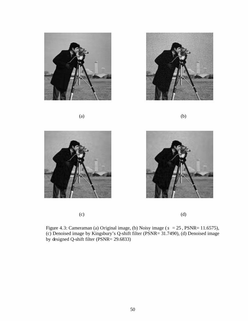
We present the original, noisy and typical denoised images of three test images

in Figures 4.1, 4.2, 4.3. Denoising results in these figures show that Kingsbury’s Q-shift

filter’s performance is better than the Q-shift filter designed in this work.

As mentioned in Section 3.6 the difference between the results of both designed

Q-shift filters are related to the method that has been used for magnitude minimization

of 2LH in designing procedure. Kingsbury’s method of minimization is on the energy of

2LH whereas we minimize the peak magnitude of 2LH . This difference may be the

reason for better PSNR results of Kingsbury’s Q-shift filters.

47

Table 4.1: Averaged PSNR values (in dB) of denoised images for different noisy images

Images

Noisy Image

Designed

Q-shift Filter

Kingsbury’s Q-shift Filter

Boat 10=σ 13.63 33.49 34.34 15=σ 13.45 31.08 32.21 20=σ 13.20 29.33 30.74 25=σ 12.90 27.87 29.69 30=σ 12.56 26.77 28.81

Baboon 10=σ 15.38 28.76 29.51 15=σ 15.09 26.61 27.59 20=σ 14.73 25.07 26.18 25=σ 14.31 23.77 25.14 30=σ 13.83 22.79 24.27

Cameraman 10=σ 12.21 35.19 36.53 15=σ 12.07 32.66 34.34 20=σ 11.88 30.99 32.89 25=σ 11.65 29.68 31.74 30=σ 11.40 28.70 30.85

48

(a)

(b)

(c)

(d)

Figure 4.1: Boat: (a) Original image, (b) Noisy image ( 10=σ , PSNR= 13.6335), (c) Denoised image by Kingsbury’s Q-shift filter (PSNR= 34.3487), (d) Denoised image by designed Q-shift filter (PSNR= 33.4932)

49

(a)

(b)

(c)

(d)

Figure 4.2: Baboon (a) Original image, (b) Noisy image ( 15=σ , PSNR= 15.0952), (c) Denoised image by Kingsbury’s Q-shift filter (PSNR= 27.5924), (d) Denoised image by designed Q-shift filter (PSNR= 26.6104)

50

(a)

(b)

(c)

(d)

Figure 4.3: Cameraman (a) Original image, (b) Noisy image ( 25=σ , PSNR= 11.6575), (c) Denoised image by Kingsbury’s Q-shift filter (PSNR= 31.7490), (d) Denoised image by designed Q-shift filter (PSNR= 29.6833)

51

Chapter 5

5 CONCLUSION AND FUTURE WORK

This work is concerned with the design of filter for DT CWT structure.

Introducing the DT CWT structure and its properties that provide shift invariance and

directional selectivity of filter banks with a limit redundancy a new design of Q-shift

filters is presented. The Q-shift filter is motivated by Kingsbury’s work for improving

orthogonality and symmetry properties. In this work we complemented Kingsbury’s

approach with a new method of designing.

Considering the requirements of Q-shift filters such as no aliasing, perfect

reconstruction, orthogonality, group delay of 1/4 sample, good smoothness and finite

support in (-2p/3, 2p/3), a new design of Q-shift filter via parameterization method is

proposed. With this method the space of orthonormal filter banks is parameterized and

the parameters are used in designing filter with desirable properties. The constraints that

have been used in this method guaranteed two vanishing moments of wavelets.

In designing of both Q-shift filters for obtaining the group delay of 1/4 and 3/4

samples the 4L tap, linear phase and symmetric low pass filter ( 2LH ) have been used.

52

For obtaining the desirable property of 1/4 and 3/4 sample period we minimized the peak

magnitude of 2LH in [p/3, p] instead of minimizing energy used by Kingsbury [9].

Results of designing are shown that the desirable mentioned properties are

obtained for the Q-shift filter. The designed Q-shift filter is compared with Kingsbury’s

Q-shift approach according to analyticity measurement, shift invariance and half-sample

delay, which are the most important properties of wavelet filters in dual-tree filter banks.

The designed Q-shift filter is applied in image denoising. Three standard image

that corrupted by an additive Gaussian noise are used. The Bivariate shrinkage algorithm

is employed for wavelet coefficient modeling and thresholding. The performance

(PSNR) of Kingsbury’s Q-shift filter (L= 14) is better than that of the designed filter (L=

14) in this work. Both filters have the same performance in visual.

The difference between results related the optimization method that has been

used in this method. Kingsbury minimized the energy of 2LH in the [p/3, p] and we

minimized the peak magnitude of 2LH in this work.

The most important reason of using the mentioned method of designing Q-shift

filter in this work is that the method has perfect orthogonality whereas Kingsbury’s

approach is approximate. It guarantees two vanishing moments by using simple

constraints and using a simple method of optimization.

53

As a future work we can explore other image applications where the designed

filters may be of advantages due to the small peak error property.

54

REFERENCES

[1] N. G. Kingsbury, ’’The dual-tree complex wavelet transform: A new technique for

shift invariance and directional filters,’’ in Proceeding of the th8 IEEE DSP

Workshop, Utah, paper no. 86, 9-12 Aug 1998.

[2] I. W. Selesnick, R. G. Baruniuk, and N. G. Kingsbury, ’’The Dual-tree complex

transform- a coherent framework for multiscale signal and image processing.’’ IEEE

Signal Processing Mag., vol.6, pp. 123-151, Nov 2005.

[3] I. W. Selesnick, ’’Hilbert transform pairs of wavelet bases’’, IEEE Signal Processing

Letters, vol. 8, no. 6, pp.170-173, Jun 2001.

[4] R. Yu and H. Ozkaramanli, ’’Hilbert transform pairs of orthogonal wavelet bases:

Necessary and sufficient conditions’’, IEEE Trans. on Signal Processing, vol. 53, no.

12, pp. 4723-4725, Dec 2005.

[5] M. Antonini, M. Barlaud, P. Mathieu and I. Daubechies, ’’Imaging coding using

wavelet transform’’, IEEE Trans. on Image Processing, vol. 1, pp. 205-220, Apr.

1992.

[6] I. W. Selesnick, ’’The Design of approximate Hilbert transform pairs of wavelet

bases’’, IEEE Trans. on Signal Processing, vol. 50, no.5, pp. 1144-1152, May 2002.

55

[7] N. G. Kingsbury, ’’The dual-tree complex wavelet transform with improved

orthogonality and symmetry properties’’, in Proc. IEEE Int. Conf. Image Processing,

Vancouver, BC, Canada, vol. 2, pp. 375-378, 10-13 Sep 2000.

[8] N. G. Kingsbury, ’’Complex wavelets for shift invariance analysis and filtering of

signals’’, Applied and Computational Harmonic Analysis, vol. 10, no. 3, pp. 234-

253, May 2001.

[9] N. G. Kingsbury, ’’Design of q-shift complex wavelets for image processing using

frequency domain energy minimization’’, In Proc. of IEEE Int. Conf. Image

Processing, Barcelona, vol. 1, pp. 1013-1016, Sep 2003.

[10] B. G. Sherlock and D. M. Monro, ’’On the space of orthonormal wavelets’’, IEEE

Trans. Signal Process, vol. 46, no. 6, pp. 1716-1720, Jun 1998.

[11] H. M. Paiva, M. N. Martins, R. K. Galvao and J. P. M. Paiva, ’’On the space of

orthonormal wavelets: Additional constraints to ensure two vanishing moments’’,

IEEE Signal Processing Letters, vol. 16, no. 2, pp. 101-104, Feb 2009.

[12] C. Sidney Burrus, R.A Gopinath and Haitao Guo, ’’Introduction to Wavelets and

Wavelet Transforms’’ Prentice Hall, New Jersy, 1998.

56

[13] R. Yu and A. Baradarani, ’’Sampled-data design of FIR dual filter banks for dual-

tree complex wavelet transform’’, IEEE Trans. on Signal Processing, vol. 56, pp.

3369-3375, Jun 2008.

[14] R. Yu, ’’Characterization and sampled-data design of dual-tree filter banks for

Hilbert transform pairs of wavelet bases’’, IEEE Trans. on Signal Processing, vol.

55, pp. 2458-2471, Jun 2007.

[15] N. G. Kingsbury, ’’Dual Tree Complex Wavelets’’, HASSIP Workshop,

Cambridge, Sep 2004.

[16] R. Yu, ’’A new shift-invariance of discrete –time systems and its application to

discrete wavelet transform analysis’’, IEEE Trans. on Signal Processing., vol. 57, no.

7, July 2009.

[17] M. Unser and T. Blue, ’’Mathematical properties of the JPEG2000 wavelet filters’’,

IEEE Trans. on Image Processing, vol. 12, pp. 1080-1090, Sep 2003.

[18] A. Baradarani and R. Yu, ’’A dual-tree complex wavelet with application in image

denoising’’, in Proceeding of the IEEE Int. conf. on Signal Processing and

Communication, Dubai, UAE, pp. 1203-1206, Nov 2007.

[19] L. Sendur and I. W. Selesnick, ’’Bivariate shrinkage with local variance

estimation’’, IEEE Signal Processing Letters, vol. 9, pp. 438-441, Dec 2002.

57

[20] L. Sendur and I. W. Selesnick, ’’Bivariate shrinkage functions for wavelet-based

denoising exploiting inter scale dependency’’, IEEE Trans. on Signal Processing,

vol. 50, pp. 2744-2756, Nov 2002.

[21] I. W. Selesnick, Matlab Implementation of Wavelet Transforms,

http://taco.poly.edu/WaveletSoftware/