A Design of Automatic Dish-Antenna Positioning System for ...

A Design of Automatic Dish-Antenna Positioning System for

Receiving Geo-Satellites Signals

EMAD ADDEEN ABDUL GABBAR MOHAMMED ALHASAN OSMAN

M.Sc in Computer Engineering and Networks, University of Gezira, 2006.

A Thesis

Submitted to the University of Gezira in Fulfillment of the Requirements for

Award of the Degree of Doctor of Philosophy

in

Telecommunication Engineering

Department of Electronics Engineering

Faculty of Engineering and Technology

May/2018

ii




Supervision Committee

Name Position Signature

Dr. Abdullahi Akode Othman Main Supervisor ……………….

Dr. Magdi Baker Mahmoud Amien

Co-supervisor ………………

May/2018

iii




Examination Committee:

Name Position Signature

Dr. Abdullahi Akode Othman Chair Person …………………….

Prof. Khalid Hamid Bilal Abdallah External Examiner …………………….

Dr. Sally Dafa-Allah Awadelkriem Internal Examiner …………………….

Date of Examination: 13/May/2018

iv

ACKNOWLEDGEMENTS

I express my deep thanks to my GOD ALLAH for

giving me the ability to complete this work.

Grateful to my supervisor Dr. Abdullahi Akode

Othman.

Grateful to my co-supervisor Dr. Magdi Baker

Mahmoud Amien.

v

DEDICATION

This research is dedicated to

My father.

The soul of my mother.

My brothers and sisters.

My beloved wife.

My son Mohammed and daughters; Ragad and Rafa.

All my dear; friends and colleagues.

vi




ABSTRACT

Geostationary satellite is a professional way to increase the TV broadcasting coverage. In

some times the site maybe within a coverage area of different satellites. To enjoy the services

provided by these satellites, a positioning system must be used to navigate between these

satellites directing the dish-antennas to the intended satellite in a short time with high

precision. Previous studies in dish-antenna positioning problem considered two factors

(azimuth and elevation) using different methods and techniques. In this research the

polarization factor was also considered. The research aims to design a dish-antenna

positioning system that allows the navigation between satellites using an easy-to-use and

effective remote-control positioning system. The designed system uses the antenna site data

(latitude, longitude) and the intended sub-satellite point (longitude) as inputs. Then it

calculates the azimuth and elevation as well as polarization angles and transforms the

calculated angles to real angles by using stepper-motors to direct the dish-antenna to the

intended satellite. The positioning system was developed and verified in two main phases. In

the first phase a mathematical model was generated based on assumption and the calculation

sequence stated above. In this phase a general relationship between stepper motor and the dish

antenna was developed to improve the positioning system efficiency. The second step in the

first phase was mathematical model simulation and validation. In the second phase the

simulated mathematical model was transformed into a real model. The real model designed

consists of two parts, software design and hardware design, based on microcontroller Arduino

Uno card, stepper-motors and IR-remote control which was used for entering satellite

longitudes and user control commands, to direct the dish-antenna. The micro-controller

provides the control signals to the motors drivers to direct the antenna. The real model was

tested using different sites data (longitude, latitude) for different locations in Sudan (Wad

Medani, Um-Durman, Port-Sudan and Kassala). The real model results illustrate that the

model achieves the azimuth/elevation positioning process in high precision. The highest

azimuth difference-average (miss-alignment) was 0.28° obtained in Kassla with gain-loss up

to -0.4255dB. Also the highest elevation difference-average was 0.28° obtained in Um-

Durman with gain-loss up to -0.4255dB. For the polarization, the highest difference-average

was 0.25° obtained in Wad Medani with miss-matching loss up to -0.000043dB. The designed

positioning system improves the directing time. It takes 40 seconds to achieve the intended

position when compared with previous studies where minimum directing time was 3 minutes.

In addition to that the designed system uses a small size microcontroller board, avoids tuning

complexity when compared with the similar system. The research recommended,

implementing the system in the southern hemisphere by modifying the mathematical model

specifically the azimuth angle and settings. Also recommends studying the dish-antenna

weight and mechanical part deeply in the design process.

vii

تصميم نظام توجيه تلقائي لهوائي إستقبال اإلشارات التلفزيونية من األقمار الصناعية

عماد الدين عبد الجبار محمد الحسن عثمان

دراسةال ملخص

األقمار الصناعية هي إحدى الطرق المستخدمة لزيادة مساحة البث التلفزيوني. في بعض األحيان قد تقع بعض المناطق

لمستخدم من اإلستمتاع ومشاهدة القنوات الفضائية التي ان األقمار الصناعية. وحتى يتمكن البث الخاص بعدد مفي مجال

فترة الهوائي بصورة دقيقة وفي هتبث عبر هذه األقمار. كان ال بد من توفر نظام تحكم يمكن من التنقل بين األقمار وتوجي

والراسي Azimuth الهوائيات في البعدين األفقي هالمجال على توجيزمنية قصيرة. عملت عدة دراسات سابقة في هذا

Elevation دون األخذ في اإلعتبار عملية ضبط اإلستقطاب الخاص باإلشارات المستقبلة Polarization هدفت هذه .

عية التي يقع في الصنا الدراسة الي تصميم نظام تحكم عن بعد يسمح للمستخدم بتوجيه هوائي اإلستقبال والتنقل بين األقمار

نطاق بثها بطريقة فعالة ودقيقة وسهلة اإلستخدام. يعتمد النظام المصمم على إحداثيات موقع الهوائي وإحداثي القمر

ياضية رظام بتحويل هذه الزوايا من قيم المستهدف في عمليات حساب الزوايا )األفقي والراسي واألستقطاب( ومن ثم يقوم الن

قية )وذلك باستخدام موتورات الخطوة( تخلص الي توجية الهوائي في إتجاه القمر المستهدف. تم تصميم الي إتجاهات حقي

هذا النظام في مرحلتين. إحتوت المرحلة األولى على النموذج الرياضي الذي تم تطويره بناء على الفرضيات والمعادالت

الخطوة حركاتط بين مواصفات الهوائي المستخدم ومالرياضية. في هذه المرحلة تم إيجاد عالقة رياضية عامة ترب

. أيضا في هذه المرحلة تم عمل محاكاة للنظام المصمم ةة عالياءهذه العالقة تضمن عمل النظام بكفالمستخدمة في هذا النظام.

ي الي الرياض موذجكما تم التحقق من صحة النظام وإمكانية تطبيقه. في المرحلة الثانية من الدراسة تم تحويل محاكاة الن

نموذج حقيقي. إحتوى النموذج على شفرة البرنامج الذي يعمل على التحكم في النظام المصمم، كما إحتوى على المكونات

الخطوة وجهاز تحكم عن بعد. يستخدم النموذج حركاتمو ARDUINO-Unoالمادية المتمثلة في متحكمة أردوينو انو

جهاز التحكم عن بعد كوحدة إدخال يعمل على إدخال إحداثي القمر المستهدف الي المتحكمة والتي بدورها تعمل على إجراء

إحداثيات مالعمليات الحسابية الالزمة ومن ثم توفر إشارات التحكم الالزمة لتوجية الهوائي. تم إختبار هذا النموذج بإستخدا

عدد من المواقع في السودان )ودمدني و أمدرمان وكسال وبورتسودان(. أظهرت نتائج هذه اإلختبارات أن النموذج المصمم

يعمل على إنجاز عملية التوجيه في البعدين األفقي والرأسي بدقة عالية، حيث كانت أعلى قيمة متوسط إنحراف في البعد

. و كانت أعلى قيمة متوسط 0.4255dB-نة كسال وكانت قيمة الفاقد في الكسب هي سجلت في مدي °0.28األفقي هي

. أما 0.4255dB-سجلت في مدينة أمدرمان وكانت قيمة الفاقد في الكسب هي °0.28إنحراف في البعد الرأسي هي

-الفاقد في الكسب هي سجلت في مدينة ودمدني وكانت قيمة °0.25ستقطاب فقد كانت أعلى قيمة متوسط إنحراف هيإلا

0.000043dB ثانية 04. كما أظهرت نتائج اإلختبارات أن النموذج عمل على توجيه الهوائي في فترة زمنية ال تزيد عن

غير معقدة مقارنة باألنظمة األخرى. أوصت استخدامه لتقنية دقائق فضال عن 3مقارنة بالدراسات السابقة التي تستغرق

النموذج في النصف الجنوبي من الكرة األرضية كما اوصت بدراسة مواصفات الهوائي والمواصفات الدراسة بتطبيق هذا

الميكانيكية للنموذج بصورة أكثر عمقا.

viii

LIST OF CONTENTS ACKNOWLEDGEMENTS .................................................................................................... iv

DEDICATION ......................................................................................................................... v

ABSTRACT ........................................................................................................................... vi

ABSTRACT IN ARABIC .................................................................................................... vii

LIST OF CONTENTS .......................................................................................................... viii

LIST OF TABLES ................................................................................................................ xiv

LIST OF FIGURES ............................................................................................................... xv

LIST OF ABBREVIATIONS ............................................................................................ xviii

CHAPTER ONE ...................................................................................................................... 1

1 INTRODUCTION ........................................................................................................ 1

1.1 BACKGROUND ...................................................................................................... 1

1.2 PROBLEM STATEMENT ....................................................................................... 2

1.3 OBJECTIVES ........................................................................................................... 2

1.4 ORGANIZATION OF THE THESIS ....................................................................... 2

CHAPTER TWO ..................................................................................................................... 4

2 LITERATURE REVIEW ............................................................................................. 4

2.1 Communications Satellite ......................................................................................... 4

2.1.1 Types of Satellite ............................................................................................... 4

High Elliptical Orbiting Satellite (HEO) ....................................................... 4

Middle-Earth Orbiting Satellite (MEO) ......................................................... 5

Low-Earth Orbiting Satellite (LEO) .............................................................. 5

Geostationary Orbit Satellite (GEO) .............................................................. 5

2.1.1.4.1 Geometric Distances ................................................................................. 5

2.1.2 Polarization of Satellite Signal .......................................................................... 8

ix

Circular Polarization ...................................................................................... 8

Linear Polarization ......................................................................................... 9

2.2 Antenna ................................................................................................................... 11

2.2.1 Dish-Antenna ................................................................................................... 11

Dish-Antenna Types .................................................................................... 12

Dish-Antenna Gain ...................................................................................... 15

Dish-antenna Beam-Width ........................................................................... 17

2.3 Stepper Motors ........................................................................................................ 18

2.3.1 Types of Stepping Motors ............................................................................... 20

Permanent-magnet (PM) .............................................................................. 20

Variable-reluctance (VR) ............................................................................. 21

2.3.1.2.1 Multi-Stack Variable-Reluctance ........................................................... 21

2.3.1.2.2 Single-stack variable-reluctance stepping motors .................................. 24

Hybrid stepping motors ................................................................................ 25

2.3.2 Operation Mode ............................................................................................... 27

One-Phase-On Full Operation Mode ........................................................... 28

Two-Phase-On Full Operation Mode ........................................................... 29

Half-step Operation Mode ........................................................................... 29

Micro-stepping Operation Mode .................................................................. 30

2.3.3 Choosing a Motor ............................................................................................ 31

Variable Reluctance versus Permanent Magnet or Hybrid .......................... 31

Hybrid versus Permanent Magnet ................................................................ 31

2.3.4 Other Stepping Motors .................................................................................... 32

2.4 Motion Control Systems ......................................................................................... 33

2.4.1 Merits of Electric Systems ............................................................................... 33

x

2.4.2 Motion Control Classification ......................................................................... 33

Closed-Loop System .................................................................................... 33

Open-Loop Motion Control Systems ........................................................... 34

2.5 Previous Related Studies ......................................................................................... 36

CHAPTER THREE ............................................................................................................... 44

3 METHODOLOGY ..................................................................................................... 44

3.1 Theoretical model development processes ............................................................. 45

3.1.1 Assumptions and Arrangements ...................................................................... 45

3.1.3 Mathematical Model ........................................................................................ 45

Azimuth and elevation part .......................................................................... 45

Polarization Part ........................................................................................... 49

Combination of Azimuth, Elevation and Polarization ................................. 50

3.1.2.3.1 Digits to Pulse Transformation ............................................................... 52

3.1.2.3.2 Operation Estimated Time ...................................................................... 52

3.1.2.3.3 System Position Precision Calculation ................................................... 53

3.2 Simulation Model .................................................................................................... 55

3.2.1 Simulation Tests .............................................................................................. 57

Equations Validation .................................................................................... 57

Positioning Accuracy Insurance ................................................................... 57

Maximum Positioning Time ........................................................................ 57

3.3 Designed Model ...................................................................................................... 57

3.3.1 Hardware Design and Requirements ............................................................... 58

Hardware and Components .......................................................................... 58

3.3.1.1.1 Computer ................................................................................................ 58

3.3.1.1.2 Arduino Uno R3 Card ............................................................................ 59

xi

3.3.1.1.3 IR-remote Control .................................................................................. 59

3.3.1.1.4 IR-Receiver ............................................................................................. 59

3.3.1.1.5 Stepper-Motor Drivers ............................................................................ 59

3.3.1.1.6 Stepper-Motors ....................................................................................... 60

3.3.1.1.7 Limit Switches ........................................................................................ 61

Entire System Wiring ................................................................................... 61

3.3.2 Software Design and Requirements ................................................................. 62

System Software .......................................................................................... 62

3.3.2.1.1 Arduino tools .......................................................................................... 63

3.3.2.1.2 Arduino C ............................................................................................... 63

System-Driver Modelling ............................................................................ 63

3.3.2.2.1 Setup function ......................................................................................... 63

3.3.2.2.2 Loop function ......................................................................................... 64

3.3.2.2.3 IR-remote Control Decoder function ...................................................... 64

3.3.2.2.4 Satellite Longitude Digits Function:....................................................... 64

3.3.2.2.5 Operation Confirm Function .................................................................. 65

3.3.2.2.6 Counter Reset function ........................................................................... 66

3.3.2.2.7 Calculations Function ............................................................................. 67

3.3.2.2.8 Back to Reference Function ................................................................... 68

3.3.2.2.9 Reset Satellite Function .......................................................................... 69

3.4 Experimental Test ................................................................................................... 70

3.4.1 Unit Testing ..................................................................................................... 70

3.4.2 Model Integration ............................................................................................ 70

3.5 System Validation ................................................................................................... 70

CHAPTER FOUR ................................................................................................................. 71

xii

4 RESULTS AND DISCUSSIONS .............................................................................. 71

4.1 Theoretical Results .................................................................................................. 71

4.2 Simulation Model Results ....................................................................................... 72

4.2.1 Equations Validation ....................................................................................... 72

4.2.2 Positioning Accuracy Insurance ...................................................................... 73

4.2.3 Maximum Positioning Time Results ............................................................... 77

First site (14.39°N, 33.52°E) ........................................................................ 77

Second site (14.323°N, 33.553°E) ............................................................... 77

4.2.4 Simulation Results Summary .......................................................................... 78

4.3 Model Experimental Setup and Results .................................................................. 78

First site (14.38°N, 33.52°E) Wad Medani: ................................................. 79

Second Site (15.638°N, 32.495°E) Um-Durman: ........................................ 80

The third site (19.61°N, 37.22°E) Port-Sudan: ............................................ 81

The fourth site (15.449°N, 36.39°E) Kassala: ............................................. 82

4.3.2 Model Integration ............................................................................................ 83

4.4 Designed System Validation ................................................................................... 84

4.4.1 Designed System in Contrast with Satsig.net and satlex.de Calculations ....... 84

First site (14.38°N, 33.52°E) Wad Medani .................................................. 84

Second Site (15.638°N, 32.495°E) Um-Durman ......................................... 86

Third site (19.61°N, 37.22°E) Port-Sudan ................................................... 87

Fourth site (15.449°N, 36.39°E) Kassala ..................................................... 89

4.4.2 Comparison between the Designed System and Related Studies .................... 91

CHAPTER FIVE ................................................................................................................... 92

CONCLUSIONS AND RECOMMENDATIONS ................................................................ 92

5.1 Conclusions ............................................................................................................. 92

xiii

5.2 Recommendations ................................................................................................... 92

6 References .................................................................................................................. 94

7 Appendixes ................................................................................................................. 97

7.1 Appendix [A] .......................................................................................................... 97

7.2 Appendix [B]........................................................................................................... 99

7.3 Appendix [C]......................................................................................................... 100

7.4 Appendix [D] ........................................................................................................ 102

7.5 Appendix [E] ......................................................................................................... 104

7.6 Appendix [F] ......................................................................................................... 105

xiv

LIST OF TABLES

TABLE 2.1 RELATIONSHIP BETWEEN WINDING CURRENT AND POLE FIELD DIRECTIONS

(ACARNLEY, 2007) .......................................................................................................... 26

TABLE 2.2 SUMMARIZATION OF THE RELATED STUDIES ........................................................ 42

TABLE 3.1 THE PROPERTIES OF THE USED LAPTOP ................................................................. 58

TABLE 3.2 THE JK1545 STEPPER MOTOR DRIVER PROPERTIES .............................................. 60

TABLE 3.3 STEPPER MOTORS PROPERTIES ............................................................................. 60

TABLE 4.1 THE RESULTS OF SATCALC-LITE IN CONTRAST WITH DESIGNED-SOFTWARE ON THE

SITE (14.39 °N, 33.52 °E) ............................................................................................... 72

TABLE 4.2 THE RESULTS OF SATCALC-LITE IN CONTRAST WITH DESIGNED-SOFTWARE ON

THE SITE (14.323°N, 33.553°E) ...................................................................................... 73

TABLE 4.3 SIMULATION CALCULATED ANGLE AND NEAREST ANGLE PROVIDED BY STEPPER

MOTOR-DRIVERS OPERATED IN HALF-STEPPING MODE (0.9°) ....................................... 74

TABLE 4.4 SIMULATION CALCULATED ANGLE AND NEAREST ANGLE PROVIDED BY STEPPER

MOTOR-DRIVERS OPERATE IN MICRO-STEPPING MODE (0.18°) ..................................... 75

TABLE 4.5 ESTIMATED TIME FOR DIRECTING ANTENNA STARTING FROM REFERENCE POINT

TO THE FARTHEST VISIBLE SATELLITE IN THE CLARKE-BELT ......................................... 77

TABLE 4.6 ESTIMATED TIME FOR DIRECTING ANTENNA STARTING FROM REFERENCE POINT

TO THE FARTHEST VISIBLE SATELLITE IN THE CLARKE-BELT ......................................... 77

TABLE 4.7 MODEL TEST READINGS IN (14.38°N, 33.52°E) SITE WITH ADJUSTING THE STEP

ANGLE TO 0.18° AND TIME DELAY TO 10MS ................................................................... 79







TABLE 7.1 THE STEPPER-MOTOR OPERATION CASES ............................................................. 102

TABLE 7.2 THE EFFECT OF AZIMUTH AND ELEVATION MISS-ALIGNMENT ANGLE REPRESENTED

AS A GAIN-LOSS FOR DISH-ANTENNA WITH HPBW ≈ 3°................................................. 105

xv

LIST OF FIGURES

FIGURE 1.2.1 GEOMETRY OF LOOK ANGLES (KOLAWOLE, 2002) ............................................. 6

FIGURE 2.2 CIRCULAR POLARIZED SIGNAL (BALANIS, 2005) .................................................... 9

FIGURE 2.3 VERTICAL AND HORIZONTAL POLARIZED SIGNALS (ELBERT, 2008) ....................... 9

FIGURE 2.4 RELATIVE RECEIVED POWER AS A TRUE RATIO FOR THE VERTICAL AND

HORIZONTAL POLARIZATION ANGLE OF THE RECEIVING ANTENNA IS ROTATED (ELBERT,

2008) ............................................................................................................................... 11

FIGURE 2.5 FOCAL POINT OF PARABOLIC ANTENNA (LWIN AND WIN, 2014) ......................... 12

FIGURE 2.6 PRIME FOCUS FEED PARABOLIC ANTENNA (DIDACTIC, 2015) ............................. 13

FIGURE 2.7 OFFSET-FEED PARABOLIC ANTENNA (DIDACTIC, 2015) ...................................... 13

FIGURE 2.8 CASSEGRAIN ANTENNA (MILLIGAN, 2005) .......................................................... 15

FIGURE 2.9 GREGORIAN ANTENNA (MILLIGAN, 2005) ........................................................... 15

FIGURE 2.10 TYPICAL ANTENNA GAIN VERSUS DISH SIZE (0.5 M TO 32 M, EFFICIENCY FACTOR

= 0.6) (DIDACTIC, 2015) .................................................................................................. 16

FIGURE 2.11 TYPICAL ANTENNA GAIN VERSUS DISH SIZE (UP TO 2 M, EFFICIENCY FACTOR =

0.6) (DIDACTIC, 2015) ..................................................................................................... 17

FIGURE 2.12 3DB (HALF-POWER BEAM WIDTH) VERSUS DISH SIZE (EFFICIENCY FACTOR =0.6)

(DIDACTIC, 2015). ........................................................................................................... 18

FIGURE 2.13 FORCE COMPONENTS BETWEEN TWO MAGNETICALLY PERMEABLE (ACARNLEY,

2007). .............................................................................................................................. 19

FIGURE 2.14 PERMANENT MAGNET (PM) STEPPER MOTOR (GRANT, 2005)........................... 20

FIGURE 2.15 THREE-STACK VARIABLE-RELUCTANCE STEPPING MOTOR CUTAWAY VIEW

(ACARNLEY, 2007) .......................................................................................................... 22

FIGURE 2.16 A- CROSS-SECTION OF A THREE-STACK VARIABLE-RELUCTANCE STEPPING

MOTOR PARALLEL TO THE SHAFT (ACARNLEY, 2007) .................................................... 23

FIGURE 2.17 CROSS-SECTION OF A SINGLE-STACK VARIABLE-RELUCTANCE STEPPING MOTOR

PERPENDICULAR TO THE SHAFT (ACARNLEY, 2007) ....................................................... 24

FIGURE 2.18 SIDE VIEW AND CROSS-SECTIONS OF THE HYBRID STEPPING MOTOR

(ACARNLEY, 2007) .......................................................................................................... 26

FIGURE 2.19 COMMERCIAL HYBRID STEPPING MOTOR (ACARNLEY, 2007) ........................... 27

FIGURE 2.20 ONE-PHASE-ON STEPPER-MOTOR OPERATION (THERAJA AND THERAJA, 2006) 28

file:///D:/Desktop%2023-9-2018/Full%20Research/Full%20research%2017-10-2018.docx%23_Toc527542594

xvi

FIGURE 2.21 TRUTH TABLES OF 2-PHASE OPERATING FULL STEP AND HALF STEPPING MODES

(THERAJA AND THERAJA, 2006) ...................................................................................... 29

FIGURE 2.22 HALF-STEP OPERATION MODE (THERAJA AND THERAJA, 2006) ........................ 30

FIGURE 2.23 CONFIGURATIONS OF THE ELECTRO-MECHANICAL AND ELECTRO-HYDRAULIC

STEPPING MOTORS (REID AND HAMID, 2006) ................................................................. 32

FIGURE 2.24 BLOCK DIAGRAM OF A BASIC CLOSED-LOOP CONTROL SYSTEM (SANDIN, 2003)

........................................................................................................................................ 34

FIGURE 2.25 MICROPROCESSOR-BASED OPEN-LOOP CONTROLS (ACARNLEY, 2007) ............ 35

FIGURE 2.26 CONSTANT STEPPING RATE OPEN-LOOP CONTROL (ACARNLEY, 2007) ............. 36

FIGURE 3.1 RESEARCH METHODOLOGY PROCESS ................................................................... 44

FIGURE 3.2 THE FOUR INTEGER CROSS POINTS SURROUND THE FLOAT CALCULATED (AZ, EL)

........................................................................................................................................ 47

FIGURE 3.3 ILLUSTRATES THE ANTENNA HORIZONTALS HPBW AND THE CALCULATED

AZIMUTH LIMITS ............................................................................................................. 48

FIGURE 3.4 (A) INTEGRATION OF AZIMUTH/ELEVATION ANGLES (B) POLARIZATION ANGLE . 50

FIGURE 3.5 THE PRODUCED PULSE CONTROL THE MOTORS MOVEMENT ............................... 52

FIGURE 3.6 SYSTEM OPERATION SEQUENCE FLOW CHART .................................................... 56

FIGURE 3.7 THE DIAGRAM OF SYSTEM MODEL ...................................................................... 58

FIGURE 3.8 THE MODEL WIRING DIAGRAM............................................................................ 62

FIGURE 3.9 THE COUNTER RESET FUNCTION FLOWCHART ..................................................... 66

FIGURE 3.10 THE CALCULATIONS FUNCTION FLOWCHART .................................................... 68

FIGURE 3.11 THE RESET SATELLITE FUNCTION FLOW-CHART ................................................ 69

FIGURE 4.1 THE RELATION BETWEEN ANTENNA DIAMETER AND STEP-ANGLE ...................... 71

FIGURE 4.2 THE POINTED AZIMUTH ANGLES AND THE HPBW LIMITS IN DEGREES ............... 74

FIGURE 4.3 THE POINTED ELEVATION ANGLES AND THE HPBW LIMITS IN DEGREES ............ 75

FIGURE 4.4 SECOND TEST POINTED AZIMUTH ANGLES AND THE HPBW LIMITS IN DEGREES 76

FIGURE 4.5 SECOND TEST POINTED ELEVATION ANGLES AND THE HPBW LIMITS IN DEGREES

........................................................................................................................................ 76

FIGURE 4.6 SYSTEM IMPLEMENTATION AND UNITS TEST ....................................................... 78

FIGURE 4.7 MODEL OF DISH-ANTENNA POSITIONING SYSTEM ............................................... 83



xvii

FIGURE 4.8 WAD MEDANI AZIMUTH MEASURED ANGLES IN CONTRAST WITH SATSIG.NET AND

SATLEX.DE RESULTS ....................................................................................................... 84

FIGURE 4.9 WAD MEDANI ELEVATION MEASURED ANGLES IN CONTRAST WITH SATSIG.NET

AND SATLEX.DE RESULTS ............................................................................................... 85

FIGURE 4.10 WAD MEDANI POLARIZATION MEASURED ANGLES IN CONTRAST WITH

SATSIG.NET AND SATLEX.DE RESULTS ............................................................................ 85

FIGURE 4.11 UM-DURMAN AZIMUTH MEASURED ANGLES IN CONTRAST WITH SATSIG.NET


FIGURE 4.12 UM-DURMAN ELEVATION MEASURED ANGLES IN CONTRAST WITH SATSIG.NET


FIGURE 4.13 UM-DURMAN POLARIZATION MEASURED ANGLES IN CONTRAST WITH


FIGURE 4.14 PORT-SUDAN AZIMUTH MEASURED ANGLES IN CONTRAST WITH SATSIG.NET


FIGURE 4.15 PORT-SUDAN ELEVATION MEASURED ANGLES IN CONTRAST WITH SATSIG.NET


FIGURE 4.16 PORT-SUDAN POLARIZATION MEASURED ANGLES IN CONTRAST WITH


FIGURE 4.17 KASSALA AZIMUTH MEASURED ANGLES IN CONTRAST WITH SATSIG.NET AND


FIGURE 4.18 KASSALA ELEVATION MEASURED ANGLES IN CONTRAST WITH SATSIG.NET AND


FIGURE 4.19 KASSALA POLARIZATION MEASURED ANGLES IN CONTRAST WITH SATSIG.NET


FIGURE 7.1 OPTIMIZING STEPPER-MOTORS DRIVERS’ OPERATION FLOWCHART .................... 103

xviii

LIST OF ABBREVIATIONS

ACU Antenna Control Unit

AM Amplitude Modulation

API Application Program Interface

API Application Program Interface

CCW Counter Clock Wise

CW Clock Wise

DC Direct Current

DSP Digital Signal Processor

FLC Fuzzy Logic Controller

FNBW First-Null Beam Width

GEO Geostationary Orbit

GPS Global Positioning System

HEO High Elliptical Orbiting

HPBW Half-Power Beam Width

IC Integrated Circuit

IDE Integrated Developer Environment

IEEE Institute of Electrical and Electronic Engineer

IR Infra-Red

LEO Low-Earth Orbiting

LHC Left Hand Circulation

LNB Low Noise Block Down-Converter

LPT Parallel Port

LQR Linear Quadratic Regulator

MEO Middle-Earth Orbiting

OPT Orbit Prediction Tracking

PC Personal Computer

PI Proportional-Integral

PID Proportional-Integral-Derivative

PLC Programmable Logic Controller

xix

PM Permanent-Magnet

PMSM Permanent Magnet Synchronous Motor

RHC Right-Hand Circulation

SSP Sub-Satellite Point

STB Set Top Box

STFLC Self-Tuning Fuzzy Logic Controller

TV Television

VR Variable-Reluctance

VRM Variable Reluctance Motors

VSAT Very Small Aperture Terminal

1

CHAPTER ONE

1 INTRODUCTION

1.1 BACKGROUND

Satellite communication is a wireless technology that is used to communicate all-around the

world. A communication satellite is an electronic communication package located in orbit

whose prime objective that is to initiate or assist communication transmission of information

from one point to another through space. Information transmitted in full-duplex (voice and

digital data) as well as in simplex (radio and television) (Kolawole, 2002).

Satellite communication involves other important communication subsystems called earth

stations. The earth station refers collectively to the equipment concerned with transmitting or

receiving signals from the satellite. The gateway through which the earth station

communicates with the satellite is the earth-station antenna. It is a transducer that coverts the

electromagnetic waves to electrical signals and vise-versa. The high altitude of some of these

satellites results in a large path loss during transmission. For this reason, a high-gain dish-

antennas were usually used for this application. Earth stations differ based on the

communication systems. It can be fixed, mobile land, airborne or sea-based (Kolawole, 2002).

Communication satellites were categorized in different types, some of them were known as

geostationary satellites that remain relatively motionless (stationary) in an apparent position

relative to the earth. Also it is called a synchronous or a geosynchronous orbit, or simply a

geosatellite (Kolawole, 2002). It is used as a professional way to increase the TV broadcast

coverage. The earth station transmits (uplink) the television program to the satellite and then

the satellite retransmits (downlink) the television program to a specific area which was known

as satellite coverage area or satellite footprint. To receive signals form a specific satellite,

direct the earth-station antenna in a specific azimuth/elevation angles (look angles) and

aligned the (LNB) with the polarization angle of the electric field of the incoming signals

(skew angle).

In general, sites can be located within the footprints of a number of satellites providing

services simultaneously. To navigate between these satellites, an antenna positioning system

must be used.

2

1.2 PROBLEM STATEMENT

The research highlights a number of problems existing in antenna positioning systems that

can be mentioned as follows:

Design complications.

Hard tuning processes.

Polarization alignment.

Significant delay in positioning process.

1.3 OBJECTIVES

The objective of this research is to design a small dish-antenna control system model for

receiving signals from geostationary satellites operating in Ku-band.

The designed model will:

Provide effective and easy-to-use positioning system.

Minimize the dish alignment-time.

Reduce the system hardware.

Provide a control system that can be embedded in (IRDs) and (STBs).

Allow the user to navigate between satellites remotely (using IR-remote control).

1.4 ORGANIZATION OF THE THESIS

The thesis consists of five chapters arranged as follows:

Chapter one contains introduction, problem definition, objectives and organization of

the thesis.

Chapter two reviews the literature that the research was based on illustrating the

concepts of the research field and the important data used to design the model’s

software/hardware components.

Chapter three discusses the methodology followed to design the model and its

verification. The explanation of the theoretical and mathematical model development

process, model simulation, real model design, experimental test and comparing the

experimental results with other sources for verifications that have been elaborated.

3

Chapter four explains and discusses the results obtained in every phase mentioned in

chapter three. In this chapter, different methods were used (figures, tables and texts)

to clarify and prove the obtained results.

Chapter five consists of the conclusions reached from the research as well as the

recommendations for future work.

And finally there are references and appendixes.

4

CHAPTER TWO

2 LITERATURE REVIEW

This chapter discusses the literature explanation of the current study. Five main titles have

been included in this chapter with their corresponding subtitles. The first title was

communications satellite which is concerned with the satellite type and some of the main

equations used in designing and modelling. The second title was the antenna; focused on the

antenna type used in the research. The third title is the stepper motors (the motors used to

position and reposition the dish-antenna). The fourth title is the motion control systems which

defines the control systems and the uses of the motors in each one. The fifth title is the related

studies which consist of different researches using different antenna positioning system

approaches.

2.1 Communications Satellite

Communications satellite is defined as a repeater station that permits users with appropriate

earth stations to exchange data and information in different formats (Elbert, 2008). New-

generation satellites are regenerative; that is, they have onboard processing capability making

them more of an intelligent unit than a mere repeater. This capability enables the satellite to

reformat received uplink data then routes the data to specified locations, or actually

regenerates data onboard the spacecraft as opposed to act simply as a relay station between

two or more ground stations (Kolawole, 2002).

2.1.1 Types of Satellite

There are, in general, four types of satellite:

High elliptical orbiting satellite (HEO)

Middle-earth orbiting satellite (MEO)

Low-earth orbiting satellite (LEO)

Geostationary satellite (GEO)

High Elliptical Orbiting Satellite (HEO)

HEO satellite is a special satellite continuously swings very close to the earth, loops out into

space, and then repeats its swing by the earth. It is an elliptical orbit almost 18,000 to

5

35,000km above the earth’s surface, not necessarily above the equator. HEOs are designed to

provide better coverage to countries with higher northern or southern latitudes (Kolawole,

2002).

Middle-Earth Orbiting Satellite (MEO)

MEO is a circular orbit satellite orbiting in the region of 8,000 to 18,000 km above the earth’s

surface, again not necessarily above the equator. MEO satellite is a compromise between the

lower orbits and the geosynchronous orbits. MEO system design involves more delays and

higher power levels than satellites in the lower orbits. However, it requires fewer satellites to

achieve the same coverage (Kolawole, 2002).

Low-Earth Orbiting Satellite (LEO)

LEO satellites orbiting the earth in networks that stretch in the region of 160 to 1,600 km

above the earth’s surface. These satellites are small, easy to launch, and lend themselves to

mass production techniques. A network of LEO satellites has the capacity to carry vast

amounts of facsimile, batch file, electronic mail and broadcast data at great speed and

communicate to end users through terrestrial links on ground-based stations. With advances

in technology, it will not be long until utility companies are accessing residential meter

readings through an LEO system or transport agencies and police are accessing vehicle plates,

monitoring traffic flow, and measuring truck weights through an LEO system (Kolawole,

2002).

Geostationary Orbit Satellite (GEO)

A geostationary orbit satellite (also known as the Clarke belt) is a circular orbit in the

equatorial plane with zero eccentricity and zero inclination (Kolawole, 2002). The satellite

remains in a fixed apparent position relative to the earth; about 22,300 miles away from the

earth if its elevation angle is orthogonal (90ᴼ) to the equator. Its revolution period is

synchronized with that of the earth in inertial space (Stonejk, 2010).

2.1.1.4.1 Geometric Distances

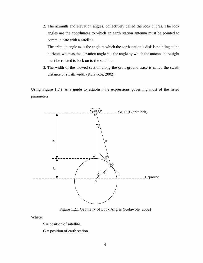
By considering the geometry of the geo-satellite’s orbit in its orbital plane, the following

will be calculated:

1. The distance between the satellite and earth station, called the slant range, Rs.

6

2. The azimuth and elevation angles, collectively called the look angles. The look

angles are the coordinates to which an earth station antenna must be pointed to

communicate with a satellite.

The azimuth angle az is the angle at which the earth station’s disk is pointing at the

horizon, whereas the elevation angle θ is the angle by which the antenna bore sight

must be rotated to lock on to the satellite.

3. The width of the viewed section along the orbit ground trace is called the swath

distance or swath width (Kolawole, 2002).

Using Figure 1.2.1 as a guide to establish the expressions governing most of the listed

parameters.

0

Equarot

Orbit (Clarke belt)

h0

M

G

Rv

Re

el

Rs

Satellite

S

Figure 1.2.1 Geometry of Look Angles (Kolawole, 2002)

Where:

S = position of satellite.

G = position of earth station.

7

Rv = OG = geocentric radius of earth at G latitude.

el = elevation angle of satellite from the earth station.

LET = latitude of the earth station. This value is positive for latitudes in the Northern

Hemisphere (i.e., north of the equator) and negative for the Southern Hemisphere (i.e.,

south of the equator).

M = location of sub-satellite point. This location’s longitude and latitude are

determined from a satellite ephemeris table. Nominally, latitude is taken as 0о for

geostationary satellite.

LSAT = latitude of the satellite.

Δ = difference in longitude between the earth station and the satellite.

γ= central angle.

r = radius of the orbit = OM + MS = Re + h0.

The central angle can be determined by using the spherical trigonometric relations as follow

(Kolawole, 2002).

γ = cos−1(sin 𝐿𝑆𝐴𝑇 sin 𝐿𝐸𝑇 + cos 𝐿𝑆𝐴𝑇 𝑐𝑜𝑠𝐿𝐸𝑇𝑐𝑜𝑠Δ) (2.1)

The slant range equation can be written as follow:

Rs = √𝑅𝑒 2 + 𝑟2 − 2rRe cos γ Km (2.2a)

Alternatively,

Rs =Rυ sin γ

cos(γ+θ) Km (2.2b)

The geocentric, Rυ, can be described by

Rυ= Re(0.99832+0.002684 cos2LET – 0.000004cos4LET …) Km (2.3)

The elevation angle el can be written as

8

𝑒𝑙 = 𝑡𝑎𝑛−1 (𝑐𝑜𝑠𝛥𝑐𝑜𝑠𝐿𝐸𝑇−(

𝑅𝑒𝑟⁄ )

√1−𝑐𝑜𝑠2𝛥 𝑐𝑜𝑠2𝐿𝐸𝑇 ) deg (2.4)

Alternatively,

𝑒𝑙 = 𝑡𝑎𝑛−1 (𝑐𝑜𝑡 𝛾 −𝑅𝜐

𝑟 𝑠𝑖𝑛 𝛾 ) deg (2.5)

and the azimuth angle is

𝑎𝑧 = 180 + tan−1 (tanΔ

sin LET) deg (2.6a)

alternatively,

𝑎𝑧 = 180 +−sinΔ

√1− cos2 LET cos2 Δ

deg (2.6b)

2.1.2 Polarization of Satellite Signal

Polarization is one of the most important properties of the propagated electromagnetic wave.

It depends on the rotation angle (angle of orientation) of the transmitting antenna. Two kinds

of polarization have been defined in satellite communication, circular and linear. Each one

has its own properties (Elbert, 2008).

Circular Polarization

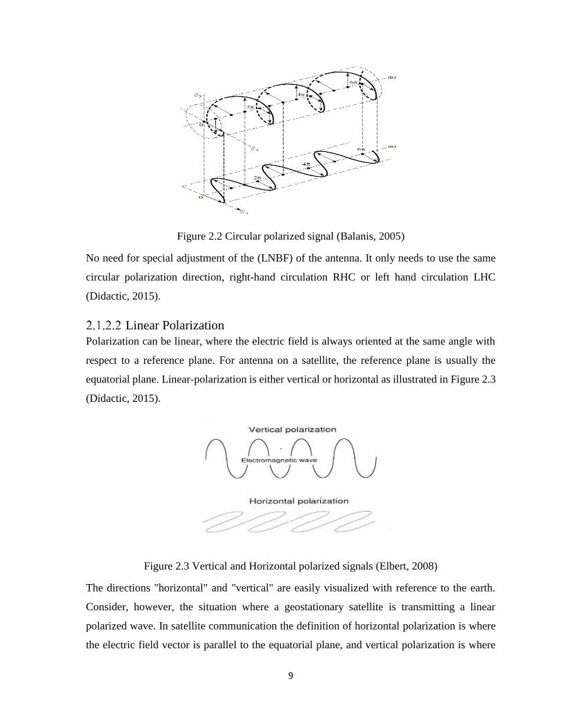
In circular or elliptical polarization, the plane of the electric field rotates with time making

one complete revolution during one period of the wave as illustrated in Figure 2.2. An

elliptically polarized wave radiates energy in all planes perpendicular to the direction of

propagation. The ratio between the maximum and minimum peaks of the electric field during

the rotation is called the axial ratio and is usually specified in decibels (Didactic, 2015).

If the rotation is clockwise, looking in the propagation direction, the polarization is called

right-hand. And if it is counterclockwise, the polarization is called left-hand (Didactic, 2015).

9

Figure 2.2 Circular polarized signal (Balanis, 2005)

No need for special adjustment of the (LNBF) of the antenna. It only needs to use the same

circular polarization direction, right-hand circulation RHC or left hand circulation LHC

(Didactic, 2015).

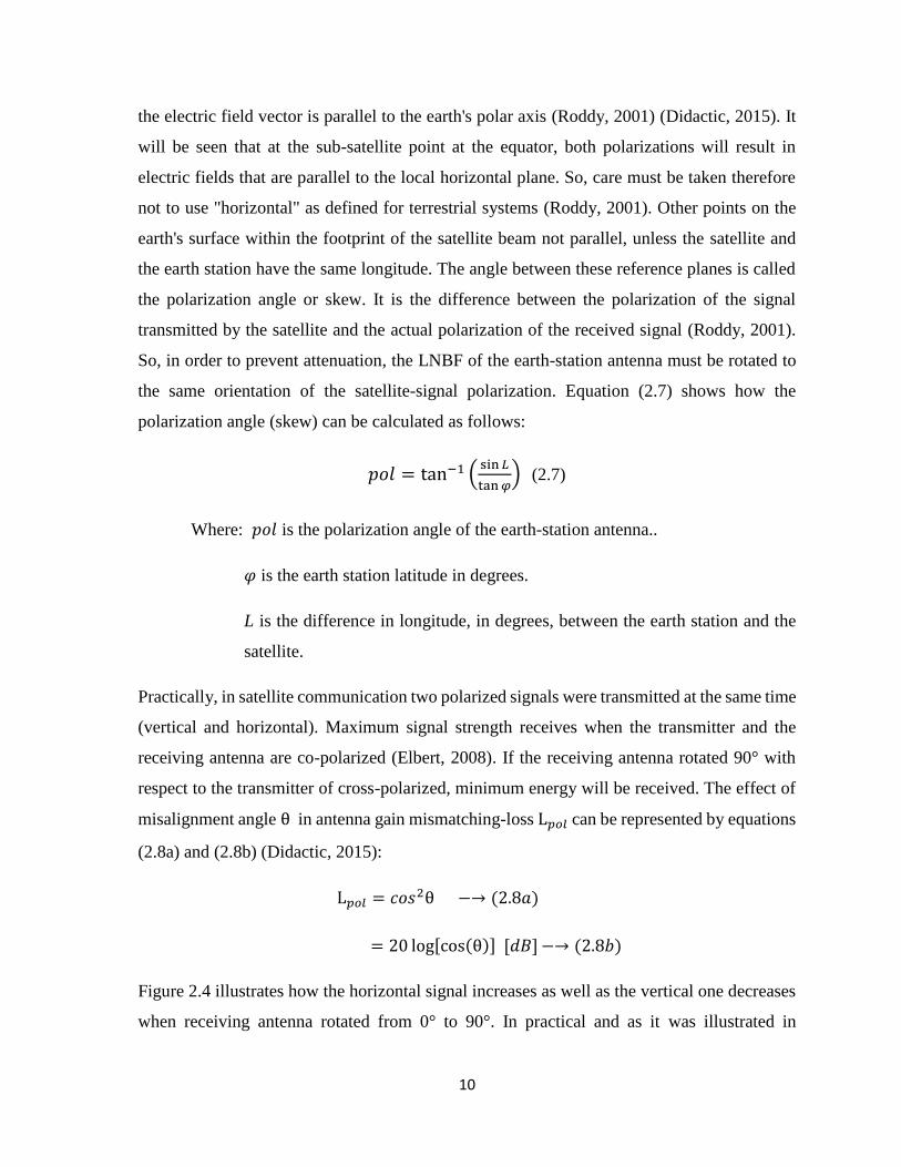
Linear Polarization

Polarization can be linear, where the electric field is always oriented at the same angle with

respect to a reference plane. For antenna on a satellite, the reference plane is usually the

equatorial plane. Linear-polarization is either vertical or horizontal as illustrated in Figure 2.3

(Didactic, 2015).

Figure 2.3 Vertical and Horizontal polarized signals (Elbert, 2008)

The directions "horizontal" and "vertical" are easily visualized with reference to the earth.

Consider, however, the situation where a geostationary satellite is transmitting a linear

polarized wave. In satellite communication the definition of horizontal polarization is where

the electric field vector is parallel to the equatorial plane, and vertical polarization is where

http://www.fpvuk.org/wp-content/uploads/2012/06/circular.png

10

the electric field vector is parallel to the earth's polar axis (Roddy, 2001) (Didactic, 2015). It

will be seen that at the sub-satellite point at the equator, both polarizations will result in

electric fields that are parallel to the local horizontal plane. So, care must be taken therefore

not to use "horizontal" as defined for terrestrial systems (Roddy, 2001). Other points on the

earth's surface within the footprint of the satellite beam not parallel, unless the satellite and

the earth station have the same longitude. The angle between these reference planes is called

the polarization angle or skew. It is the difference between the polarization of the signal

transmitted by the satellite and the actual polarization of the received signal (Roddy, 2001).

So, in order to prevent attenuation, the LNBF of the earth-station antenna must be rotated to

the same orientation of the satellite-signal polarization. Equation (2.7) shows how the

polarization angle (skew) can be calculated as follows:

𝑝𝑜𝑙 = tan−1 (sin 𝐿

tan𝜑) (2.7)

Where: 𝑝𝑜𝑙 is the polarization angle of the earth-station antenna..

𝜑 is the earth station latitude in degrees.

L is the difference in longitude, in degrees, between the earth station and the

satellite.

Practically, in satellite communication two polarized signals were transmitted at the same time

(vertical and horizontal). Maximum signal strength receives when the transmitter and the

receiving antenna are co-polarized (Elbert, 2008). If the receiving antenna rotated 90° with

respect to the transmitter of cross-polarized, minimum energy will be received. The effect of

misalignment angle θ in antenna gain mismatching-loss L𝑝𝑜𝑙 can be represented by equations

(2.8a) and (2.8b) (Didactic, 2015):

L𝑝𝑜𝑙 = 𝑐𝑜𝑠2θ −→ (2.8𝑎)

= 20 log[cos(θ)] [𝑑𝐵]−→ (2.8𝑏)

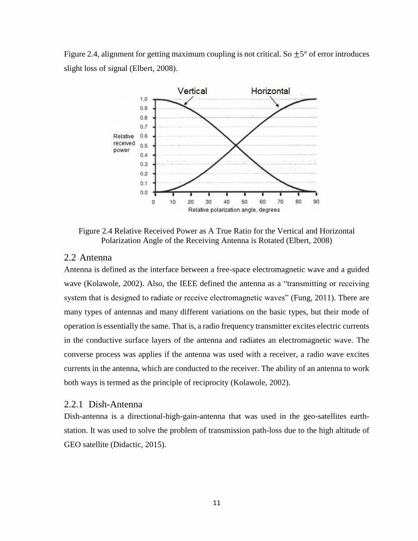
Figure 2.4 illustrates how the horizontal signal increases as well as the vertical one decreases

when receiving antenna rotated from 0° to 90°. In practical and as it was illustrated in

11

Figure 2.4, alignment for getting maximum coupling is not critical. So ±5° of error introduces

slight loss of signal (Elbert, 2008).

Figure 2.4 Relative Received Power as A True Ratio for the Vertical and Horizontal

Polarization Angle of the Receiving Antenna is Rotated (Elbert, 2008)

2.2 Antenna

Antenna is defined as the interface between a free-space electromagnetic wave and a guided

wave (Kolawole, 2002). Also, the IEEE defined the antenna as a “transmitting or receiving

system that is designed to radiate or receive electromagnetic waves” (Fung, 2011). There are

many types of antennas and many different variations on the basic types, but their mode of

operation is essentially the same. That is, a radio frequency transmitter excites electric currents

in the conductive surface layers of the antenna and radiates an electromagnetic wave. The

converse process was applies if the antenna was used with a receiver, a radio wave excites

currents in the antenna, which are conducted to the receiver. The ability of an antenna to work

both ways is termed as the principle of reciprocity (Kolawole, 2002).

2.2.1 Dish-Antenna

Dish-antenna is a directional-high-gain-antenna that was used in the geo-satellites earth-

station. It was used to solve the problem of transmission path-loss due to the high altitude of

GEO satellite (Didactic, 2015).

12

Dish-Antenna Types

Subsequent demands of reflector-antenna for uses in different applications increased the

development progress of experimental techniques and complicated analytical in shaping the

reflectors and optimizing illumination over their apertures to maximize the gain (Balanis,

2005).

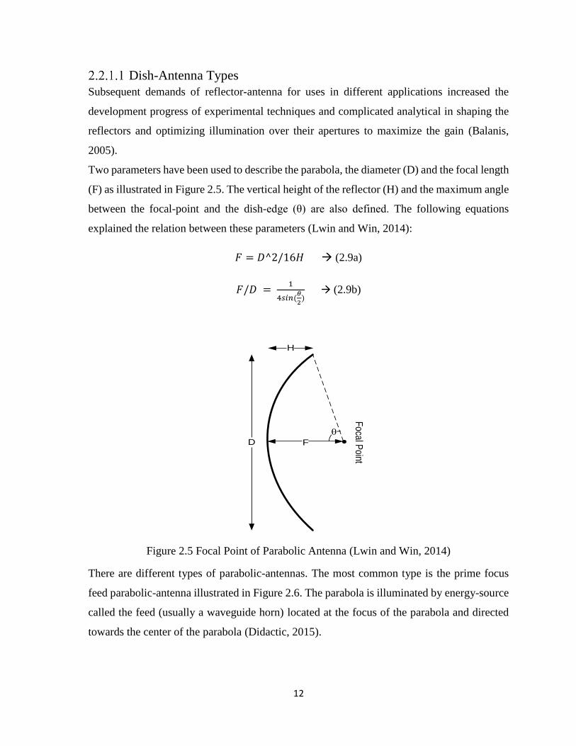
Two parameters have been used to describe the parabola, the diameter (D) and the focal length

(F) as illustrated in Figure 2.5. The vertical height of the reflector (H) and the maximum angle

between the focal-point and the dish-edge (θ) are also defined. The following equations

explained the relation between these parameters (Lwin and Win, 2014):

𝐹 = 𝐷^2/16𝐻 (2.9a)

𝐹/𝐷 = 1

4𝑠𝑖𝑛(𝜃

2) (2.9b)

D

H

F

θ

Focal P

oint

Figure 2.5 Focal Point of Parabolic Antenna (Lwin and Win, 2014)

There are different types of parabolic-antennas. The most common type is the prime focus

feed parabolic-antenna illustrated in Figure 2.6. The parabola is illuminated by energy-source

called the feed (usually a waveguide horn) located at the focus of the parabola and directed

towards the center of the parabola (Didactic, 2015).

13

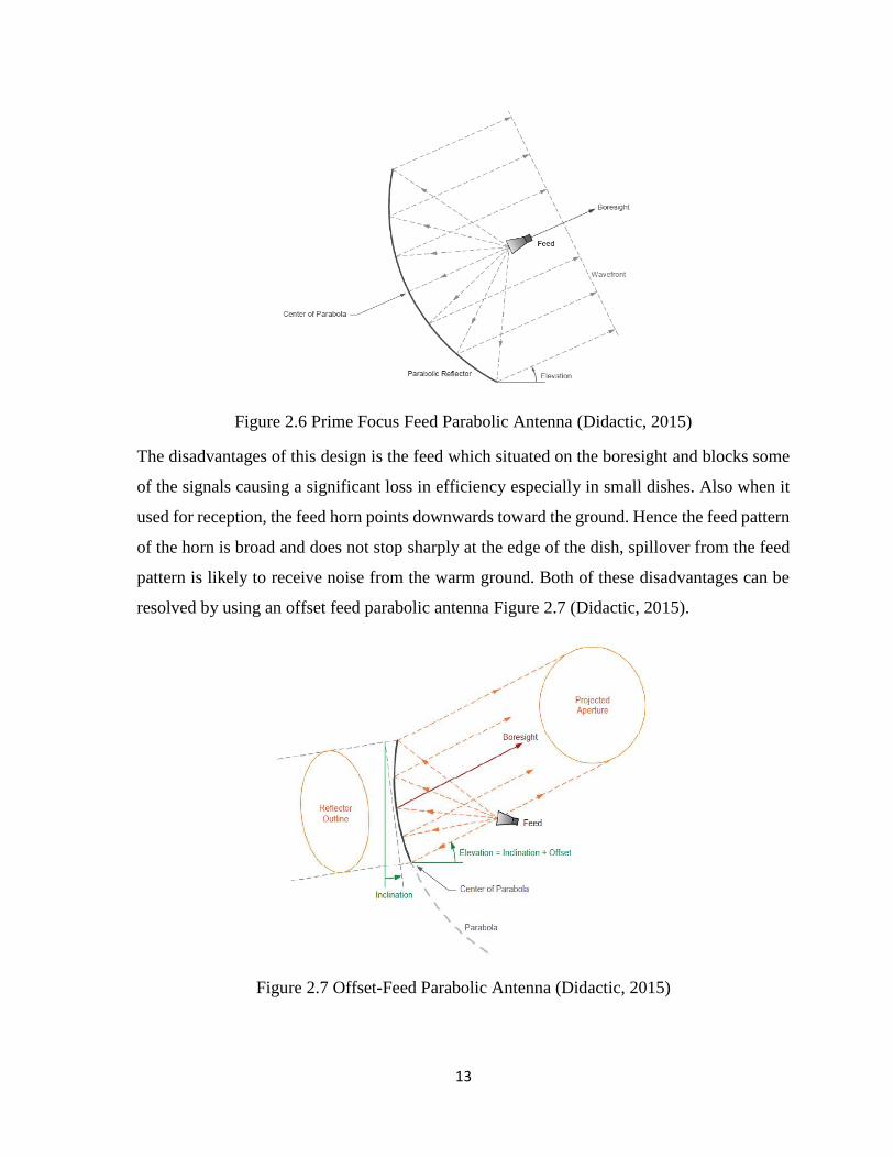
Figure 2.6 Prime Focus Feed Parabolic Antenna (Didactic, 2015)

The disadvantages of this design is the feed which situated on the boresight and blocks some

of the signals causing a significant loss in efficiency especially in small dishes. Also when it

used for reception, the feed horn points downwards toward the ground. Hence the feed pattern

of the horn is broad and does not stop sharply at the edge of the dish, spillover from the feed

pattern is likely to receive noise from the warm ground. Both of these disadvantages can be

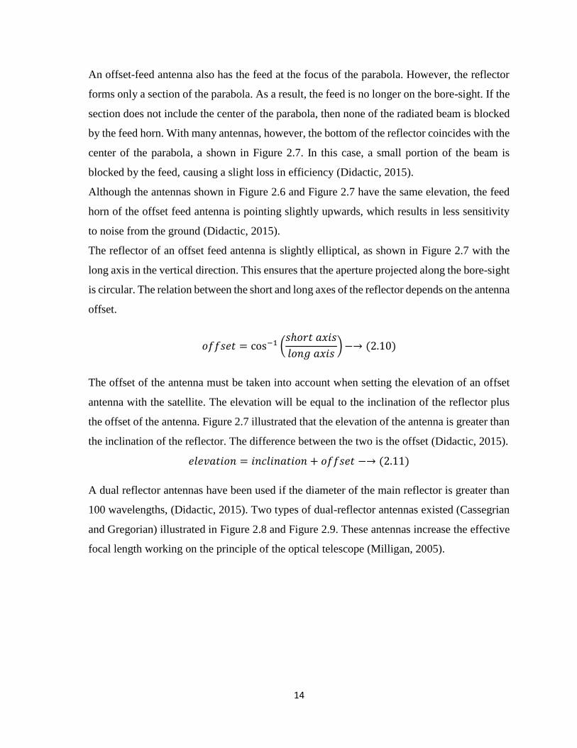
resolved by using an offset feed parabolic antenna Figure 2.7 (Didactic, 2015).

Figure 2.7 Offset-Feed Parabolic Antenna (Didactic, 2015)

14

An offset-feed antenna also has the feed at the focus of the parabola. However, the reflector

forms only a section of the parabola. As a result, the feed is no longer on the bore-sight. If the

section does not include the center of the parabola, then none of the radiated beam is blocked

by the feed horn. With many antennas, however, the bottom of the reflector coincides with the

center of the parabola, a shown in Figure 2.7. In this case, a small portion of the beam is

blocked by the feed, causing a slight loss in efficiency (Didactic, 2015).

Although the antennas shown in Figure 2.6 and Figure 2.7 have the same elevation, the feed

horn of the offset feed antenna is pointing slightly upwards, which results in less sensitivity

to noise from the ground (Didactic, 2015).

The reflector of an offset feed antenna is slightly elliptical, as shown in Figure 2.7 with the

long axis in the vertical direction. This ensures that the aperture projected along the bore-sight

is circular. The relation between the short and long axes of the reflector depends on the antenna

offset.

𝑜𝑓𝑓𝑠𝑒𝑡 = cos−1 (𝑠ℎ𝑜𝑟𝑡 𝑎𝑥𝑖𝑠

𝑙𝑜𝑛𝑔 𝑎𝑥𝑖𝑠)−→ (2.10)

The offset of the antenna must be taken into account when setting the elevation of an offset

antenna with the satellite. The elevation will be equal to the inclination of the reflector plus

the offset of the antenna. Figure 2.7 illustrated that the elevation of the antenna is greater than

the inclination of the reflector. The difference between the two is the offset (Didactic, 2015).

𝑒𝑙𝑒𝑣𝑎𝑡𝑖𝑜𝑛 = 𝑖𝑛𝑐𝑙𝑖𝑛𝑎𝑡𝑖𝑜𝑛 + 𝑜𝑓𝑓𝑠𝑒𝑡 −→ (2.11)

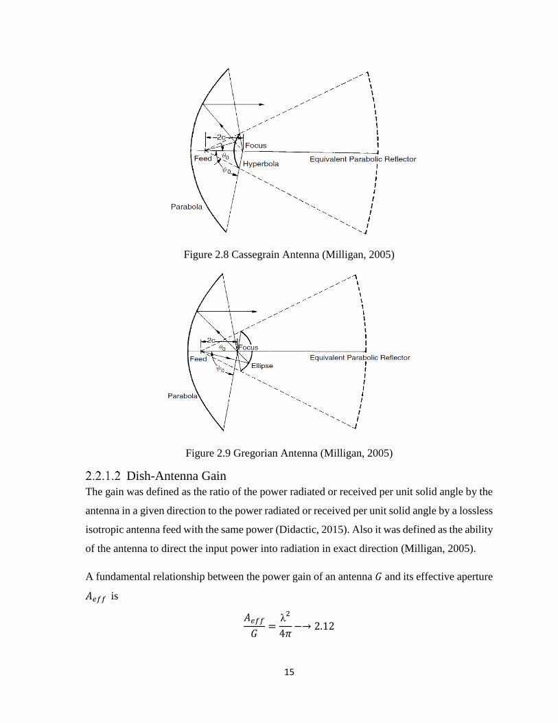
A dual reflector antennas have been used if the diameter of the main reflector is greater than

100 wavelengths, (Didactic, 2015). Two types of dual-reflector antennas existed (Cassegrian

and Gregorian) illustrated in Figure 2.8 and Figure 2.9. These antennas increase the effective

focal length working on the principle of the optical telescope (Milligan, 2005).

15

Figure 2.8 Cassegrain Antenna (Milligan, 2005)

Figure 2.9 Gregorian Antenna (Milligan, 2005)

Dish-Antenna Gain

The gain was defined as the ratio of the power radiated or received per unit solid angle by the

antenna in a given direction to the power radiated or received per unit solid angle by a lossless

isotropic antenna feed with the same power (Didactic, 2015). Also it was defined as the ability

of the antenna to direct the input power into radiation in exact direction (Milligan, 2005).

A fundamental relationship between the power gain of an antenna 𝐺 and its effective aperture

𝐴𝑒𝑓𝑓 is

𝐴𝑒𝑓𝑓

𝐺=

λ2

4𝜋−→ 2.12

16

The effective aperture 𝐴𝑒𝑓𝑓 is smaller than the physical aperture 𝐴𝑝ℎ𝑦𝑠𝑖𝑐𝑎𝑙 by a factor known

as the illumination efficiency 𝜂.

𝐴𝑒𝑓𝑓 = 𝜂𝐴𝑝ℎ𝑦𝑠𝑖𝑐𝑎𝑙 −→ 2.13

The illumination efficiency 𝜂 is usually a specified number within the range of 0.5 and 0.8.

The conventional value often used in calculation is 0.55 (Roddy, 2001).

The physical aperture 𝐴𝑝ℎ𝑦𝑠𝑖𝑐𝑎𝑙 is

𝐴𝑝ℎ𝑦𝑠𝑖𝑐𝑎𝑙 =𝜋𝐷2

4 −→ 2.14

From the relationships given by Equations (2.12) up-to (2.14), the gain is

𝐺 =4𝜋

𝜆2𝜂 𝐴𝑝ℎ𝑦𝑠𝑖𝑐𝑎𝑙−→ 2.15

= 𝜂 (𝜋𝐷

𝜆)2

−→ 2.16

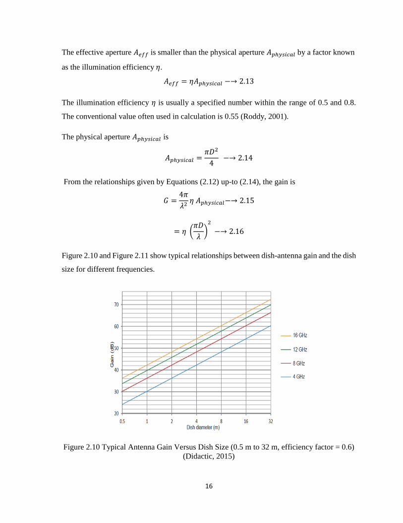
Figure 2.10 and Figure 2.11 show typical relationships between dish-antenna gain and the dish

size for different frequencies.

Figure 2.10 Typical Antenna Gain Versus Dish Size (0.5 m to 32 m, efficiency factor = 0.6)

(Didactic, 2015)

17

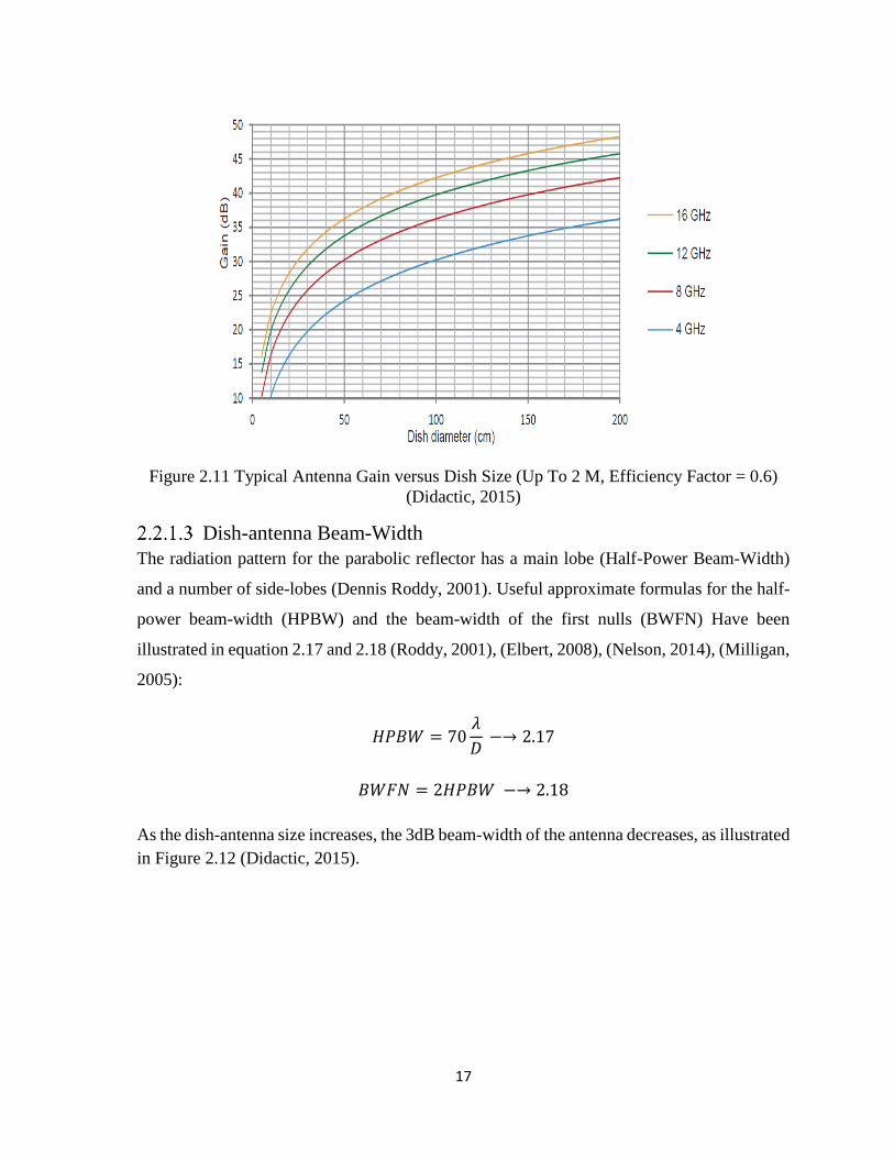
Figure 2.11 Typical Antenna Gain versus Dish Size (Up To 2 M, Efficiency Factor = 0.6)

(Didactic, 2015)

Dish-antenna Beam-Width

The radiation pattern for the parabolic reflector has a main lobe (Half-Power Beam-Width)

and a number of side-lobes (Dennis Roddy, 2001). Useful approximate formulas for the half-

power beam-width (HPBW) and the beam-width of the first nulls (BWFN) Have been

illustrated in equation 2.17 and 2.18 (Roddy, 2001), (Elbert, 2008), (Nelson, 2014), (Milligan,

2005):

𝐻𝑃𝐵𝑊 = 70𝜆

𝐷 −→ 2.17

𝐵𝑊𝐹𝑁 = 2𝐻𝑃𝐵𝑊 −→ 2.18

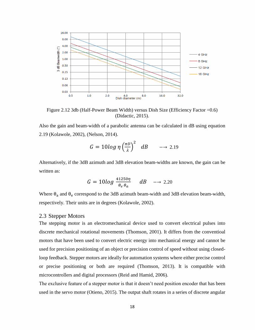
As the dish-antenna size increases, the 3dB beam-width of the antenna decreases, as illustrated

in Figure 2.12 (Didactic, 2015).

18

Figure 2.12 3db (Half-Power Beam Width) versus Dish Size (Efficiency Factor =0.6)

(Didactic, 2015).

Also the gain and beam-width of a parabolic antenna can be calculated in dB using equation

2.19 (Kolawole, 2002), (Nelson, 2014).

𝐺 = 10𝑙𝑜𝑔 𝜂 (𝜋𝐷

𝜆)2 𝑑𝐵 −→ 2.19

Alternatively, if the 3dB azimuth and 3dB elevation beam-widths are known, the gain can be

written as:

𝐺 = 10𝑙𝑜𝑔 41250𝜂

𝜃𝑒 𝜃𝑎 𝑑𝐵 −→ 2.20

Where θa and θe correspond to the 3dB azimuth beam-width and 3dB elevation beam-width,

respectively. Their units are in degrees (Kolawole, 2002).

2.3 Stepper Motors

The stepping motor is an electromechanical device used to convert electrical pulses into

discrete mechanical rotational movements (Thomson, 2001). It differs from the conventioal

motors that have been used to convert electric energy into mechanical energy and cannot be

used for precision positioning of an object or precision control of speed without using closed-

loop feedback. Stepper motors are ideally for automation systems where either precise control

or precise positioning or both are required (Thomson, 2013). It is compatible with

microcontrollers and digital processors (Reid and Hamid, 2006).

The exclusive feature of a stepper motor is that it doesn’t need position encoder that has been

used in the servo motor (Otieno, 2015). The output shaft rotates in a series of discrete angular

19

steps, one step for each time a command pulse is received. So, receiving a definite number of

pulses, cause in turning the shaft through a definite known angle (no feedback needs to be

taken to the output shaft). This feature reduces the complexity of mechanical part in designed

systems. It makes the stepper-motor well-suited for open-loop position control (Thomson,

2013).

The angle which the motor-shaft rotates for each command pulse is called step-angle β. Small

step-angle means great number of steps per revolution and high resolution or accuracy of

positioning obtained. The most common step-angle size are 1.8°, 2.5°, 7.5° and 15°.

(Thomson, 2013).

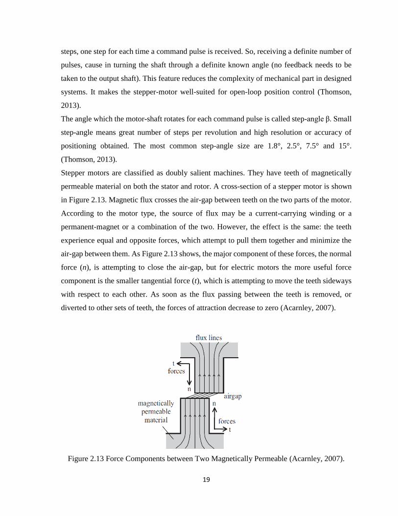
Stepper motors are classified as doubly salient machines. They have teeth of magnetically

permeable material on both the stator and rotor. A cross-section of a stepper motor is shown

in Figure 2.13. Magnetic flux crosses the air-gap between teeth on the two parts of the motor.

According to the motor type, the source of flux may be a current-carrying winding or a

permanent-magnet or a combination of the two. However, the effect is the same: the teeth

experience equal and opposite forces, which attempt to pull them together and minimize the

air-gap between them. As Figure 2.13 shows, the major component of these forces, the normal

force (n), is attempting to close the air-gap, but for electric motors the more useful force

component is the smaller tangential force (t), which is attempting to move the teeth sideways

with respect to each other. As soon as the flux passing between the teeth is removed, or

diverted to other sets of teeth, the forces of attraction decrease to zero (Acarnley, 2007).

Figure 2.13 Force Components between Two Magnetically Permeable (Acarnley, 2007).

20

2.3.1 Types of Stepping Motors

There are three basic types of stepping motors: permanent magnet, variable reluctance and

hybrid. Permanent magnet motors have a magnetized rotor, while variable reluctance motors

have toothed soft-iron rotors and hybrid stepping motors combine features of both permanent

magnet and variable reluctance motors (Condit and Jones, 2004).

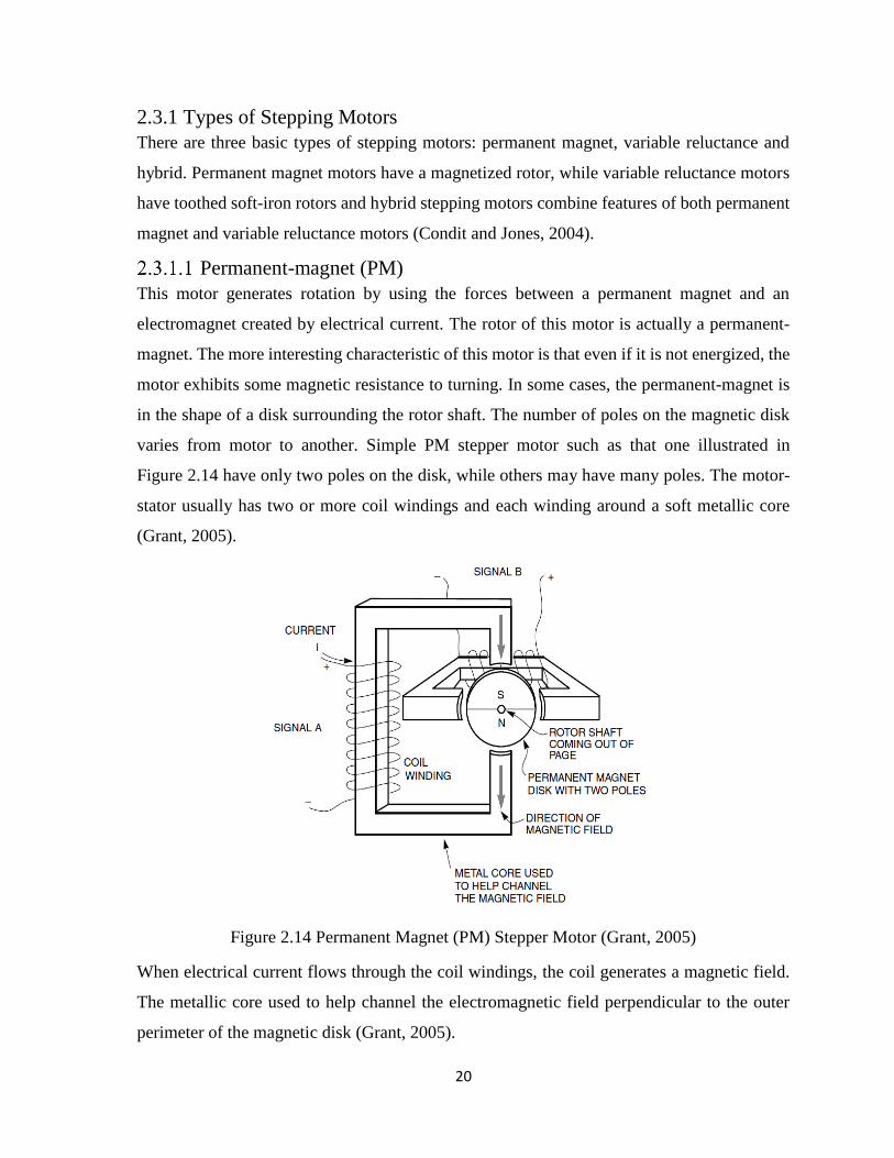
Permanent-magnet (PM)

This motor generates rotation by using the forces between a permanent magnet and an

electromagnet created by electrical current. The rotor of this motor is actually a permanent-

magnet. The more interesting characteristic of this motor is that even if it is not energized, the

motor exhibits some magnetic resistance to turning. In some cases, the permanent-magnet is

in the shape of a disk surrounding the rotor shaft. The number of poles on the magnetic disk

varies from motor to another. Simple PM stepper motor such as that one illustrated in

Figure 2.14 have only two poles on the disk, while others may have many poles. The motor-

stator usually has two or more coil windings and each winding around a soft metallic core

(Grant, 2005).

Figure 2.14 Permanent Magnet (PM) Stepper Motor (Grant, 2005)

When electrical current flows through the coil windings, the coil generates a magnetic field.

The metallic core used to help channel the electromagnetic field perpendicular to the outer

perimeter of the magnetic disk (Grant, 2005).

21

Depends on the polarity of the generated electromagnetic field in the coil and the closest

permanent magnetic field on the disk. This causes in an attraction force spinning the rotor in

a direction that lets an opposite pole on the perimeter of the magnetic disk to align itself with

the electromagnetic field generated by the coil. When the nearest opposite pole on the disk

aligns itself with the electromagnetic field generated by the coil, the rotor will break and

remain fixed in this alignment as long as the electromagnetic field from the coil is not changed

(Grant, 2005).

The value of step-angle β can be expressed either in terms of the rotor and stator poles (teeth)

Nr and Ns respectively or in terms of the number of stator phases (m) and rotor teeth as follow

(Thomson, 2013).

𝛽 =(𝑁𝑠 − 𝑁𝑟)

𝑁𝑠. 𝑁𝑟× 360° (2.22)

OR

𝛽 =360°

𝑚.𝑁𝑟=

360°

𝑁𝑜. 𝑜𝑓 𝑠𝑡𝑎𝑡𝑜𝑟 𝑝ℎ𝑎𝑠𝑒 × 𝑁𝑜. 𝑜𝑓 𝑟𝑜𝑡𝑜𝑟 𝑝ℎ𝑎𝑠𝑒 (2.23)

Variable-reluctance (VR)

There are two configurations for the variable-reluctance stepper motor (multi-stack and

single-stack), but in both cases the magnetic field is produced solely by the winding currents.

It has no permanent-magnet rotor. It has been operated on the principle of minimizing the

reluctance along the path of the applied magnetic field. When the stator coils are energized,

the rotor teeth will align with the energized stator poles. It differs from the PM stepper in that

it has no residual torque to hold the rotor at one position when turned off. (Thomson, 2013).

2.3.1.2.1 Multi-Stack Variable-Reluctance

Multi-stack variable-reluctance stepper motor is divided along its axial length into

magnetically isolated sections (‘stacks’), each of which can be excited by a separate winding

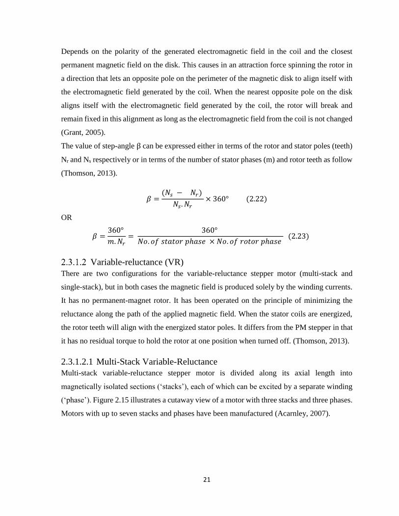
(‘phase’). Figure 2.15 illustrates a cutaway view of a motor with three stacks and three phases.

Motors with up to seven stacks and phases have been manufactured (Acarnley, 2007).

22

Figure 2.15 Three-Stack Variable-Reluctance Stepping Motor Cutaway View (Acarnley,

2007)

Each stack includes a stator, held in position by the outer-casing of the motor and carrying the

motor windings, and a rotor element. The entire rotor elements are fabricated as a single unit,

which is supported at each end of the machine by bearings and includes a projecting shaft for

the connection of external loads, as shown in Figure 2.16a. Both stator and rotor are made

from electrical steel, which is usually coated so that the magnetic fields within the motor can

change rapidly without causing excessive eddy current losses. Each stator has a number of

poles. Figure 2.16b illustrates a four poles and a part of the phase winding is coiled around

each pole to produce a radial magnetic field in the pole. Adjacent poles are coiled in the

opposite sense, so that the radial magnetic fields in adjacent poles are in opposite directions.

The complete magnetic circuit for each stack is from one stator pole, across the air-gap into

the rotor, through the rotor, across the air-gap into an adjacent pole, through this pole,

returning to the original pole via a closing section, called the ‘back-iron’. This magnetic circuit

is repeated for each pair of poles, and therefore in the example of Figure 2.16b there are four

main flux paths. The normal forces of attraction between the four sets of stator and rotor teeth

cancel each other, the resultant force between the rotor and stator arises only from the

tangential forces (Sandin, 2003).

23

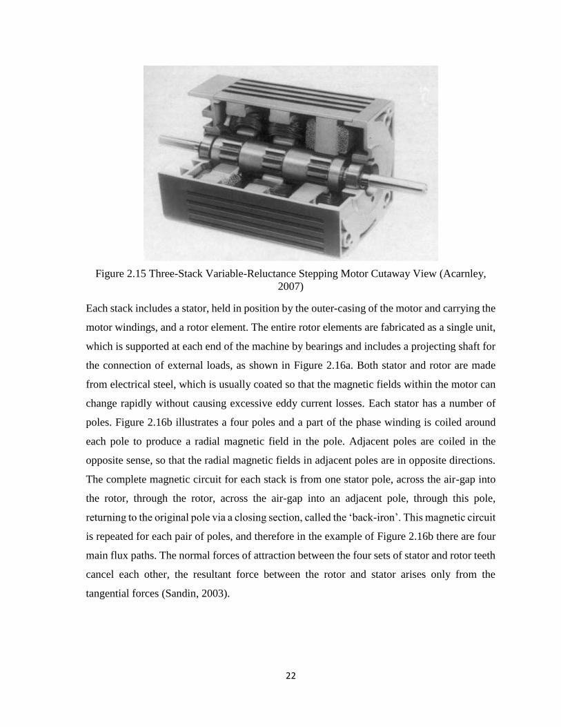
Figure 2.16 a- Cross-Section of a Three-Stack Variable-Reluctance Stepping Motor Parallel

to the Shaft (Acarnley, 2007)

b- Cross-Sections of a Three-Stack Variable-Reluctance Stepping Motor Perpendicular to

the Shaft (Acarnley, 2007)

The position of the rotor relative to the stator in a particular stack is accurately defined

whenever the phase winding is excited. Positional accuracy is achieved by means of the equal

numbers of teeth on the stator and rotor, which tend to align so as to reduce the reluctance of

the stack magnetic circuit. In the position where the stator and rotor teeth are fully aligned the

circuit reluctance is minimized and the magnetic flux in the stack is at its maximum value

(Acarnley, 2007).

The step length of a multi-stack variable-reluctance motor can be calculated based on the

numbers of stator/rotor teeth and the number of stacks. If the motor has N stacks (and phases)

the basic excitation sequence consists of each stack being excited in turn, producing a total

rotor movement of N steps. The same stack is excited at the beginning and end of the sequence

and if the stator and rotor teeth are aligned in this stack the rotor has moved one tooth pitch.

Since one tooth pitch is equal to (360/p)°, where p is the number of rotor teeth, the distance

moved for one change of excitation is

𝑠𝑡𝑒𝑝 𝑙𝑒𝑛𝑔𝑡ℎ = (360 𝑁𝑝⁄ )° (2.24)

The motor illustrated in Figure 2.16a has three stacks and eight rotor teeth, so the step length

is 15°. The step length for the multi-stack variable-reluctance stepping motor is typically in

the range (2–15)° (Acarnley, 2007).

24

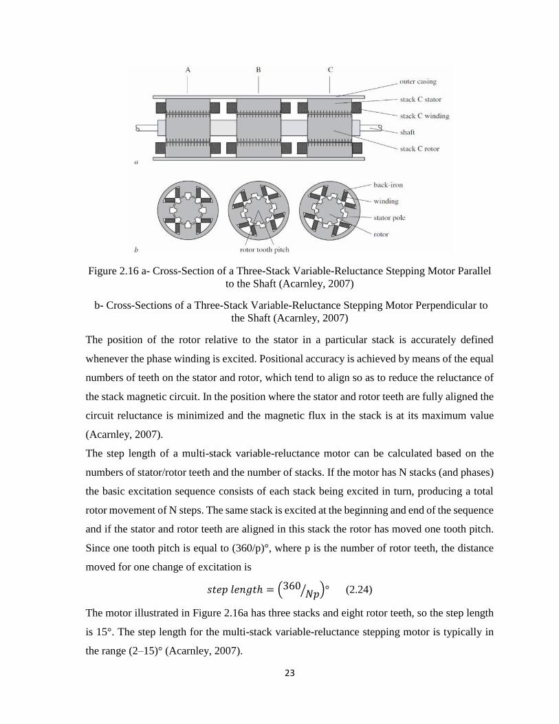
2.3.1.2.2 Single-stack variable-reluctance stepping motors

This motor is fabricated as a single unit. Its cross-section parallel to the shaft is similar to one

stack of the motor illustrated in Figure 2.15 and Figure 2.16b. The cross-section perpendicular

to the shaft has been illustrated in

Figure 2.17 (Acarnley, 2007).

Considering the stator arrangement, the stator teeth extend from the stator/rotor air-gap to the

back-iron. Each tooth has a separate winding which produces a radial magnetic field when

excited by a direct current. The motor in Figure 2.17 has six stator teeth and the windings on

opposite teeth are connected together to form one phase. So, this machine has three phases

which is the minimum number required to produce rotation in either direction. Windings on

opposite stator teeth are in opposing senses, so that the radial magnetic field in one tooth is

directed towards the air-gap whereas in the other tooth the field is directed away from the air-

gap. For one phase excited the main flux path is from one stator tooth, across the air-gap into

a rotor tooth, directly across the rotor to another rotor tooth/air-gap/stator tooth combination

and returning via the back-iron. However, it is possible for a small proportion of the flux to

leak through unexcited stator teeth. These secondary flux paths produce mutual coupling

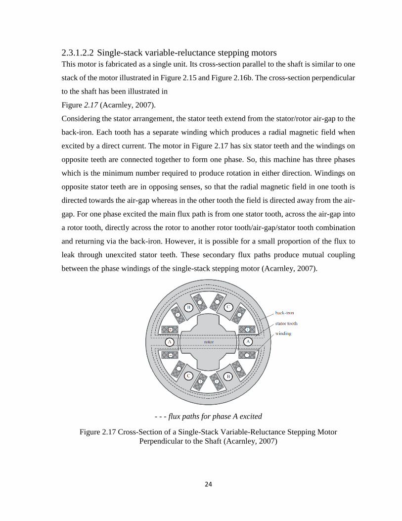
between the phase windings of the single-stack stepping motor (Acarnley, 2007).

- - - flux paths for phase A excited

Figure 2.17 Cross-Section of a Single-Stack Variable-Reluctance Stepping Motor

Perpendicular to the Shaft (Acarnley, 2007)

25

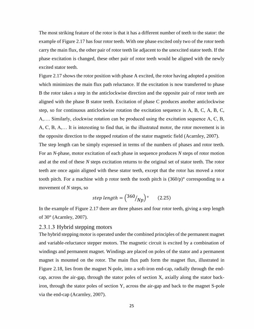
The most striking feature of the rotor is that it has a different number of teeth to the stator: the

example of Figure 2.17 has four rotor teeth. With one phase excited only two of the rotor teeth

carry the main flux, the other pair of rotor teeth lie adjacent to the unexcited stator teeth. If the

phase excitation is changed, these other pair of rotor teeth would be aligned with the newly

excited stator teeth.

Figure 2.17 shows the rotor position with phase A excited, the rotor having adopted a position

which minimizes the main flux path reluctance. If the excitation is now transferred to phase

B the rotor takes a step in the anticlockwise direction and the opposite pair of rotor teeth are

aligned with the phase B stator teeth. Excitation of phase C produces another anticlockwise

step, so for continuous anticlockwise rotation the excitation sequence is A, B, C, A, B, C,

A,…. Similarly, clockwise rotation can be produced using the excitation sequence A, C, B,

A, C, B, A,… It is interesting to find that, in the illustrated motor, the rotor movement is in

the opposite direction to the stepped rotation of the stator magnetic field (Acarnley, 2007).

The step length can be simply expressed in terms of the numbers of phases and rotor teeth.

For an N-phase, motor excitation of each phase in sequence produces N steps of rotor motion

and at the end of these N steps excitation returns to the original set of stator teeth. The rotor

teeth are once again aligned with these stator teeth, except that the rotor has moved a rotor

tooth pitch. For a machine with p rotor teeth the tooth pitch is (360/p)° corresponding to a

movement of N steps, so

𝑠𝑡𝑒𝑝 𝑙𝑒𝑛𝑔𝑡ℎ = (360 𝑁𝑝⁄ ) ° (2.25)

In the example of Figure 2.17 there are three phases and four rotor teeth, giving a step length

of 30° (Acarnley, 2007).

Hybrid stepping motors

The hybrid stepping motor is operated under the combined principles of the permanent magnet

and variable-reluctance stepper motors. The magnetic circuit is excited by a combination of

windings and permanent magnet. Windings are placed on poles of the stator and a permanent

magnet is mounted on the rotor. The main flux path form the magnet flux, illustrated in

Figure 2.18, lies from the magnet N-pole, into a soft-iron end-cap, radially through the end-

cap, across the air-gap, through the stator poles of section X, axially along the stator back-

iron, through the stator poles of section Y, across the air-gap and back to the magnet S-pole

via the end-cap (Acarnley, 2007).

26

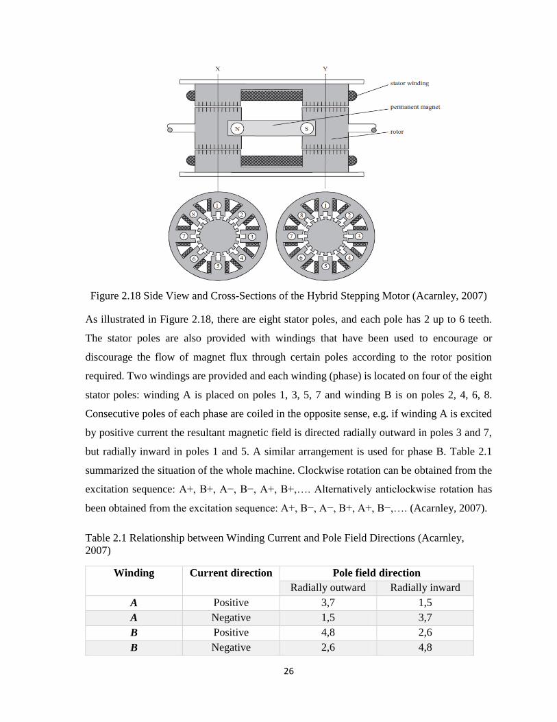
Figure 2.18 Side View and Cross-Sections of the Hybrid Stepping Motor (Acarnley, 2007)

As illustrated in Figure 2.18, there are eight stator poles, and each pole has 2 up to 6 teeth.

The stator poles are also provided with windings that have been used to encourage or

discourage the flow of magnet flux through certain poles according to the rotor position

required. Two windings are provided and each winding (phase) is located on four of the eight

stator poles: winding A is placed on poles 1, 3, 5, 7 and winding B is on poles 2, 4, 6, 8.

Consecutive poles of each phase are coiled in the opposite sense, e.g. if winding A is excited

by positive current the resultant magnetic field is directed radially outward in poles 3 and 7,

but radially inward in poles 1 and 5. A similar arrangement is used for phase B. Table 2.1

summarized the situation of the whole machine. Clockwise rotation can be obtained from the

excitation sequence: A+, B+, A−, B−, A+, B+,…. Alternatively anticlockwise rotation has

been obtained from the excitation sequence: A+, B−, A−, B+, A+, B−,…. (Acarnley, 2007).

Table 2.1 Relationship between Winding Current and Pole Field Directions (Acarnley,

2007)

Winding Current direction Pole field direction

Radially outward Radially inward

A Positive 3,7 1,5

A Negative 1,5 3,7

B Positive 4,8 2,6

B Negative 2,6 4,8

27

The step-length can be related to the number of rotor teeth, p. A complete cycle of excitation

for the hybrid motor consists of four states and produces four steps of rotor movement. The

excitation state is the same before and after these four steps, so the alignment of stator/rotor

teeth occurs under the same stator poles. Therefore four steps correspond to a rotor movement

of one tooth pitch of (360/p)° and for the hybrid motor.

𝑠𝑡𝑒𝑝 𝑙𝑒𝑛𝑔𝑡ℎ = (90 𝑝⁄ )° (2.26)

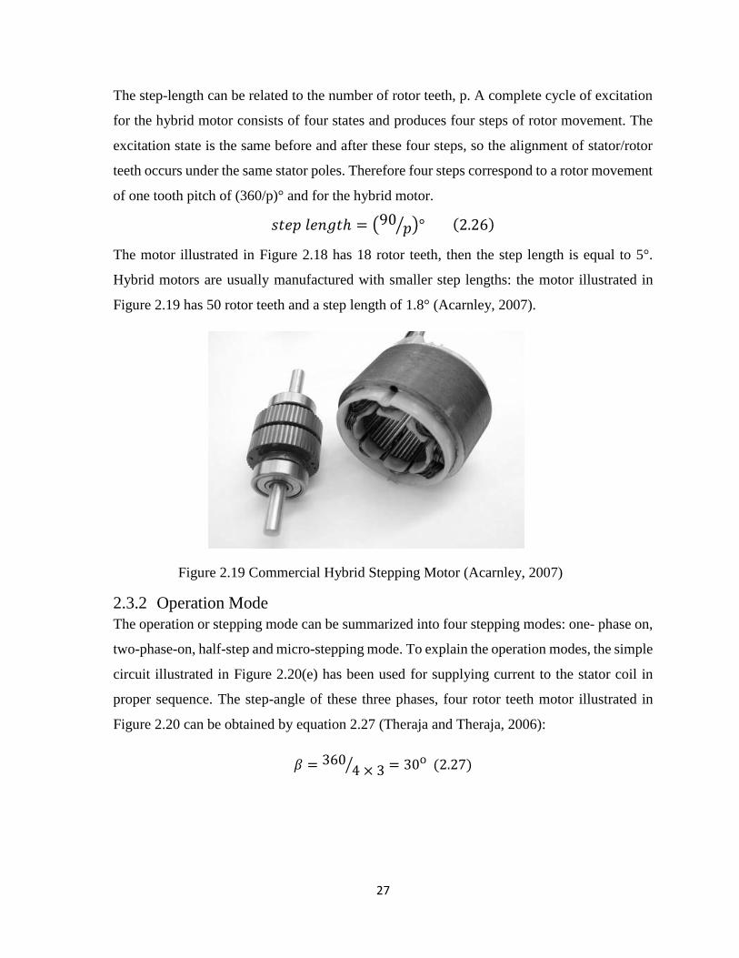
The motor illustrated in Figure 2.18 has 18 rotor teeth, then the step length is equal to 5°.

Hybrid motors are usually manufactured with smaller step lengths: the motor illustrated in

Figure 2.19 has 50 rotor teeth and a step length of 1.8° (Acarnley, 2007).

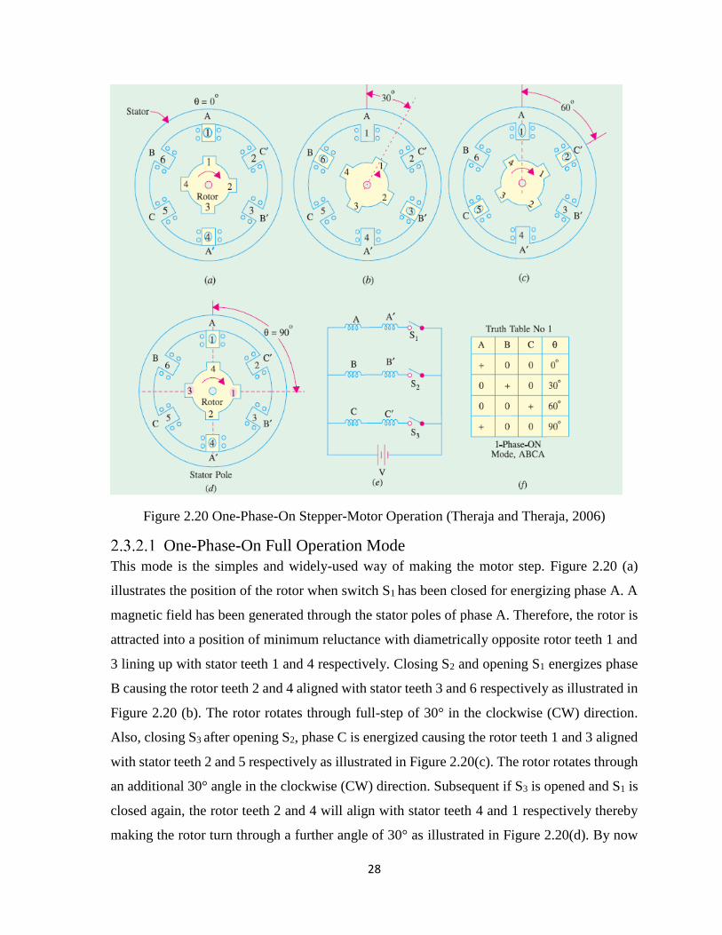
2.3.2 Operation Mode

The operation or stepping mode can be summarized into four stepping modes: one- phase on,

two-phase-on, half-step and micro-stepping mode. To explain the operation modes, the simple

circuit illustrated in Figure 2.20(e) has been used for supplying current to the stator coil in

proper sequence. The step-angle of these three phases, four rotor teeth motor illustrated in

Figure 2.20 can be obtained by equation 2.27 (Theraja and Theraja, 2006):

𝛽 = 3604 × 3⁄ = 30ᴼ (2.27)

Figure 2.19 Commercial Hybrid Stepping Motor (Acarnley, 2007)

28

Figure 2.20 One-Phase-On Stepper-Motor Operation (Theraja and Theraja, 2006)

One-Phase-On Full Operation Mode

This mode is the simples and widely-used way of making the motor step. Figure 2.20 (a)

illustrates the position of the rotor when switch S1 has been closed for energizing phase A. A

magnetic field has been generated through the stator poles of phase A. Therefore, the rotor is

attracted into a position of minimum reluctance with diametrically opposite rotor teeth 1 and

3 lining up with stator teeth 1 and 4 respectively. Closing S2 and opening S1 energizes phase

B causing the rotor teeth 2 and 4 aligned with stator teeth 3 and 6 respectively as illustrated in

Figure 2.20 (b). The rotor rotates through full-step of 30° in the clockwise (CW) direction.

Also, closing S3 after opening S2, phase C is energized causing the rotor teeth 1 and 3 aligned

with stator teeth 2 and 5 respectively as illustrated in Figure 2.20(c). The rotor rotates through

an additional 30° angle in the clockwise (CW) direction. Subsequent if S3 is opened and S1 is

closed again, the rotor teeth 2 and 4 will align with stator teeth 4 and 1 respectively thereby

making the rotor turn through a further angle of 30° as illustrated in Figure 2.20(d). By now

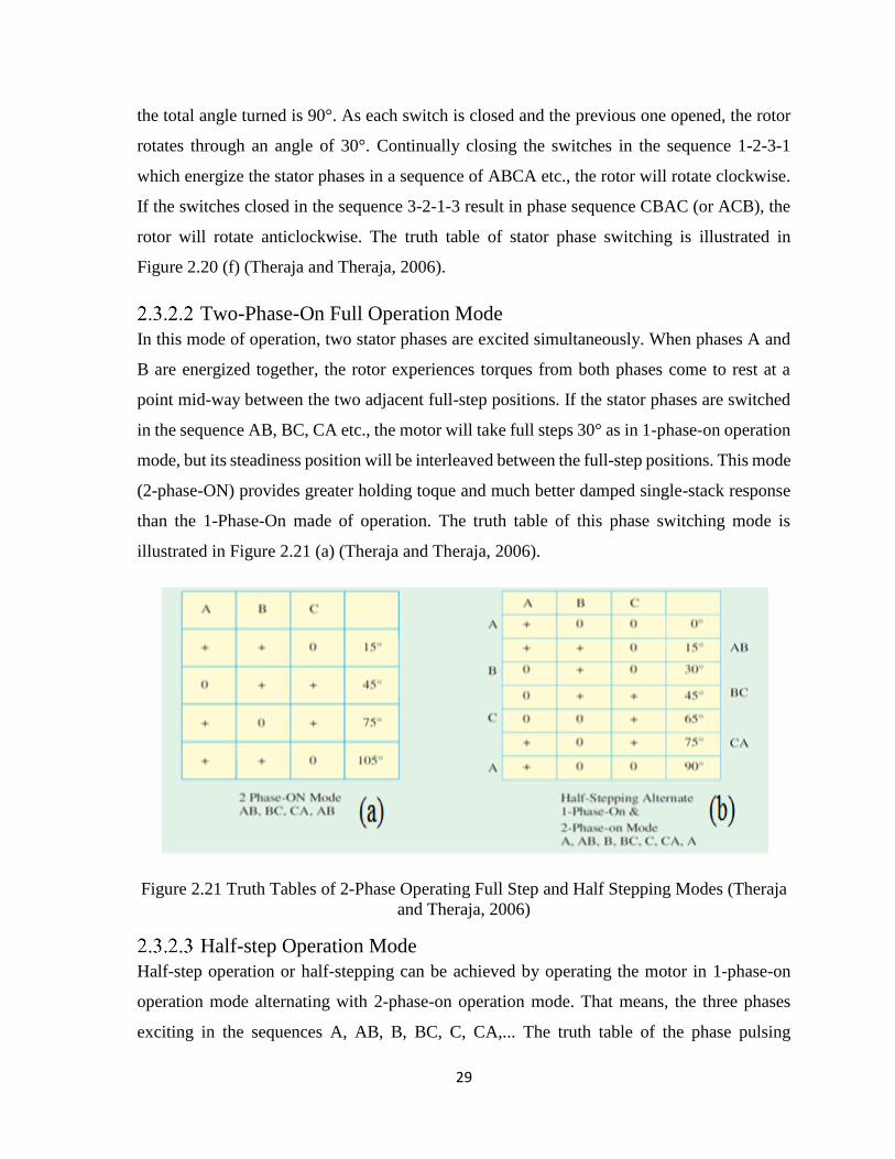
29

the total angle turned is 90°. As each switch is closed and the previous one opened, the rotor

rotates through an angle of 30°. Continually closing the switches in the sequence 1-2-3-1

which energize the stator phases in a sequence of ABCA etc., the rotor will rotate clockwise.

If the switches closed in the sequence 3-2-1-3 result in phase sequence CBAC (or ACB), the

rotor will rotate anticlockwise. The truth table of stator phase switching is illustrated in

Figure 2.20 (f) (Theraja and Theraja, 2006).

Two-Phase-On Full Operation Mode

In this mode of operation, two stator phases are excited simultaneously. When phases A and

B are energized together, the rotor experiences torques from both phases come to rest at a

point mid-way between the two adjacent full-step positions. If the stator phases are switched

in the sequence AB, BC, CA etc., the motor will take full steps 30° as in 1-phase-on operation

mode, but its steadiness position will be interleaved between the full-step positions. This mode

(2-phase-ON) provides greater holding toque and much better damped single-stack response

than the 1-Phase-On made of operation. The truth table of this phase switching mode is

illustrated in Figure 2.21 (a) (Theraja and Theraja, 2006).

Figure 2.21 Truth Tables of 2-Phase Operating Full Step and Half Stepping Modes (Theraja

and Theraja, 2006)

Half-step Operation Mode

Half-step operation or half-stepping can be achieved by operating the motor in 1-phase-on

operation mode alternating with 2-phase-on operation mode. That means, the three phases

exciting in the sequences A, AB, B, BC, C, CA,... The truth table of the phase pulsing

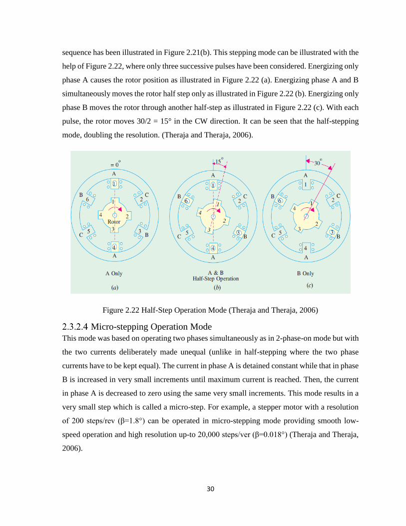
30

sequence has been illustrated in Figure 2.21(b). This stepping mode can be illustrated with the

help of Figure 2.22, where only three successive pulses have been considered. Energizing only

phase A causes the rotor position as illustrated in Figure 2.22 (a). Energizing phase A and B

simultaneously moves the rotor half step only as illustrated in Figure 2.22 (b). Energizing only

phase B moves the rotor through another half-step as illustrated in Figure 2.22 (c). With each

pulse, the rotor moves 30/2 = 15° in the CW direction. It can be seen that the half-stepping

mode, doubling the resolution. (Theraja and Theraja, 2006).

Figure 2.22 Half-Step Operation Mode (Theraja and Theraja, 2006)

Micro-stepping Operation Mode

This mode was based on operating two phases simultaneously as in 2-phase-on mode but with

the two currents deliberately made unequal (unlike in half-stepping where the two phase

currents have to be kept equal). The current in phase A is detained constant while that in phase

B is increased in very small increments until maximum current is reached. Then, the current

in phase A is decreased to zero using the same very small increments. This mode results in a

very small step which is called a micro-step. For example, a stepper motor with a resolution

of 200 steps/rev (β=1.8°) can be operated in micro-stepping mode providing smooth low-

speed operation and high resolution up-to 20,000 steps/ver (β=0.018°) (Theraja and Theraja,

2006).

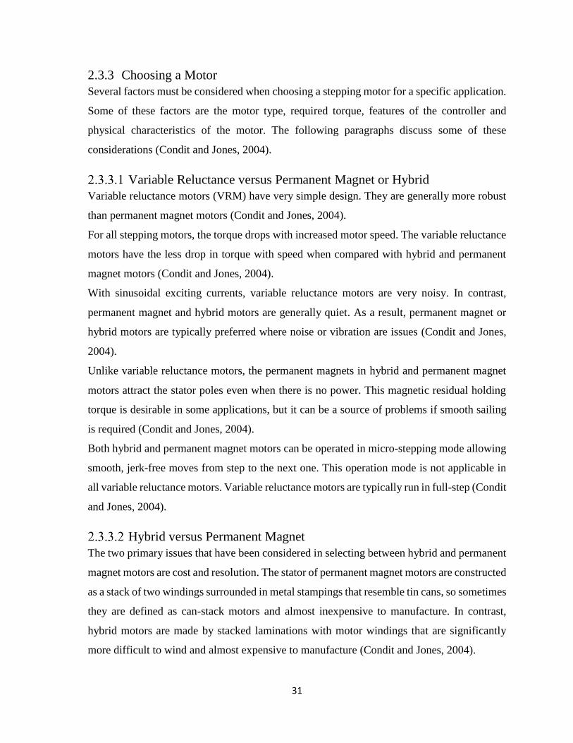
31

2.3.3 Choosing a Motor

Several factors must be considered when choosing a stepping motor for a specific application.

Some of these factors are the motor type, required torque, features of the controller and

physical characteristics of the motor. The following paragraphs discuss some of these

considerations (Condit and Jones, 2004).

Variable Reluctance versus Permanent Magnet or Hybrid

Variable reluctance motors (VRM) have very simple design. They are generally more robust

than permanent magnet motors (Condit and Jones, 2004).

For all stepping motors, the torque drops with increased motor speed. The variable reluctance

motors have the less drop in torque with speed when compared with hybrid and permanent

magnet motors (Condit and Jones, 2004).

With sinusoidal exciting currents, variable reluctance motors are very noisy. In contrast,

permanent magnet and hybrid motors are generally quiet. As a result, permanent magnet or

hybrid motors are typically preferred where noise or vibration are issues (Condit and Jones,

2004).

Unlike variable reluctance motors, the permanent magnets in hybrid and permanent magnet

motors attract the stator poles even when there is no power. This magnetic residual holding

torque is desirable in some applications, but it can be a source of problems if smooth sailing

is required (Condit and Jones, 2004).

Both hybrid and permanent magnet motors can be operated in micro-stepping mode allowing

smooth, jerk-free moves from step to the next one. This operation mode is not applicable in

all variable reluctance motors. Variable reluctance motors are typically run in full-step (Condit

and Jones, 2004).

Hybrid versus Permanent Magnet

The two primary issues that have been considered in selecting between hybrid and permanent

magnet motors are cost and resolution. The stator of permanent magnet motors are constructed

as a stack of two windings surrounded in metal stampings that resemble tin cans, so sometimes

they are defined as can-stack motors and almost inexpensive to manufacture. In contrast,

hybrid motors are made by stacked laminations with motor windings that are significantly

more difficult to wind and almost expensive to manufacture (Condit and Jones, 2004).

32

Hybrid motors can step at rates higher than permanent magnet motors. They suffer some of

the vibration problems of variable reluctance (Condit and Jones, 2004).

2.3.4 Other Stepping Motors

The latter designs of stepper motor included mechanical detecting and solenoid controls.

These designs have been replaced by more efficient and rugged designs. The latter stepper

motors have been classified as (1) permanent-magnet steppers, (2) variable-reluctance

steppers, (3) hybrid steppers, (4) electromechanical steppers, and (5) electro-hydraulic

steppers. The first three ones are already mentioned before. The electro-mechanical and

electro-hydraulic stepper motors have been illustrated in Figure 2.23 (Reid and Hamid, 2006)

Figure 2.23 Configurations of the Electro-Mechanical and Electro-Hydraulic Stepping

Motors (Reid and Hamid, 2006)

33

2.4 Motion Control Systems

A modern motion control system typically consists of a motion controller, a motor drive, an

electric motor and feedback sensors. A motion controller today can be a standalone

programmable controller, a personal computer containing a motion control card or a

programmable logic controller (PLC).

All of the components of a motion control system must work together seamlessly to achieve

their assigned functions. Selection of these components must be based on both engineering

and economic considerations (Sandin, 2003).

2.4.1 Merits of Electric Systems

Most modern motion control systems are powered by electric motors rather than hydraulic or

pneumatic motors or actuators because of the bellow benefits that they offer:

Simple designing, programming and installing.

Extra precise load positioning.

High flexibility, efficiency and capacity.

Few product or process defects.

Clean and quiet operation without any oil or air leakage.

Low maintenance costs (Sandin, 2003).

2.4.2 Motion Control Classification

Motion control systems can be classified as closed-loop or open-loop. A closed-loop system

requires feedback sensors that measure the output variables and provide error-correcting

signals. In contrast, an open-loop system does not require any measurements of output

variables (Sandin, 2003).

Closed-Loop System

A closed-loop motion control system block diagram illustrated in Figure 2.24, has one or more

feedback loops that continuously compare the system’s response with input commands or

settings to correct errors in: motor speed, position and torque as well as load position.

Feedback sensors provide the electronic signals for correcting deviations from the desired

input commands. Closed-loop systems are also called servo-systems (Sandin, 2003).

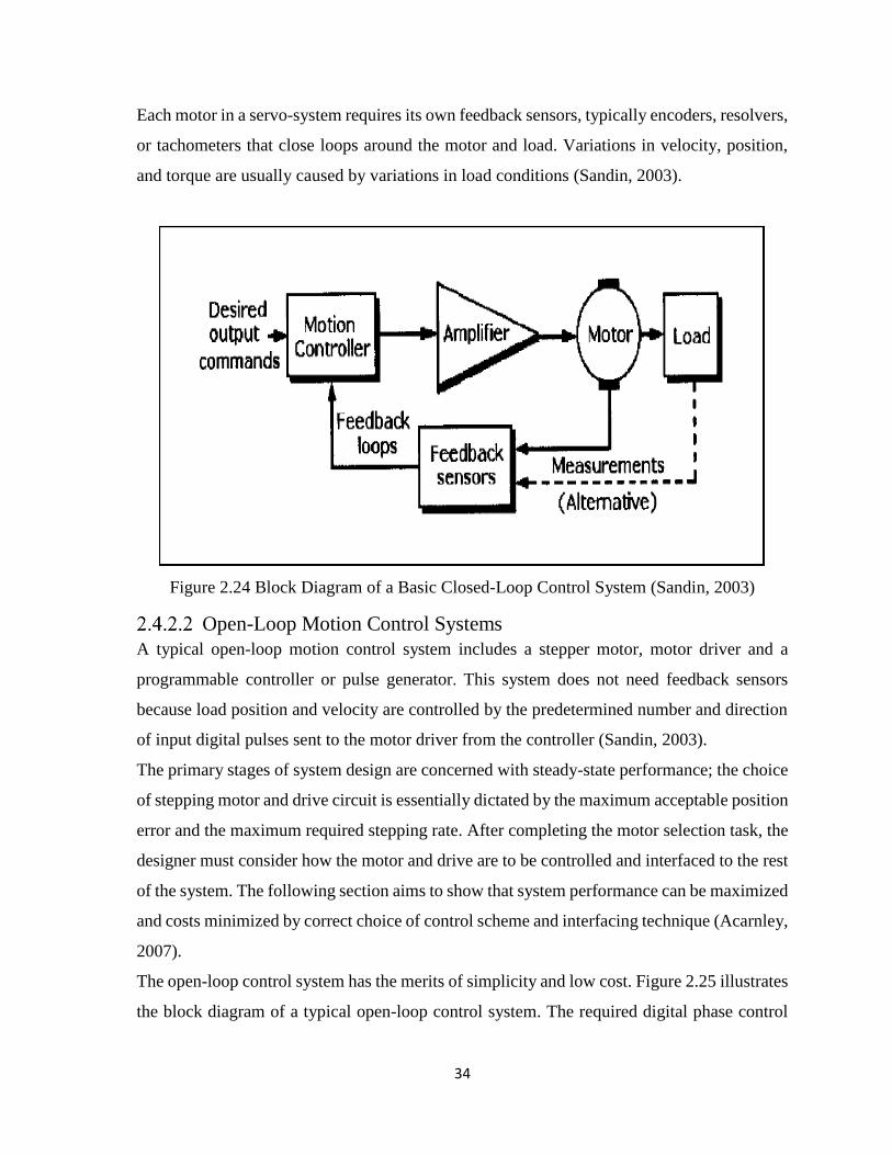
34

Each motor in a servo-system requires its own feedback sensors, typically encoders, resolvers,

or tachometers that close loops around the motor and load. Variations in velocity, position,

and torque are usually caused by variations in load conditions (Sandin, 2003).

Figure 2.24 Block Diagram of a Basic Closed-Loop Control System (Sandin, 2003)

Open-Loop Motion Control Systems

A typical open-loop motion control system includes a stepper motor, motor driver and a

programmable controller or pulse generator. This system does not need feedback sensors

because load position and velocity are controlled by the predetermined number and direction

of input digital pulses sent to the motor driver from the controller (Sandin, 2003).

The primary stages of system design are concerned with steady-state performance; the choice

of stepping motor and drive circuit is essentially dictated by the maximum acceptable position

error and the maximum required stepping rate. After completing the motor selection task, the

designer must consider how the motor and drive are to be controlled and interfaced to the rest

of the system. The following section aims to show that system performance can be maximized

and costs minimized by correct choice of control scheme and interfacing technique (Acarnley,

2007).

The open-loop control system has the merits of simplicity and low cost. Figure 2.25 illustrates

the block diagram of a typical open-loop control system. The required digital phase control

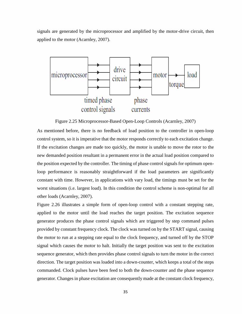
35

signals are generated by the microprocessor and amplified by the motor-drive circuit, then

applied to the motor (Acarnley, 2007).

Figure 2.25 Microprocessor-Based Open-Loop Controls (Acarnley, 2007)

As mentioned before, there is no feedback of load position to the controller in open-loop

control system, so it is imperative that the motor responds correctly to each excitation change.

If the excitation changes are made too quickly, the motor is unable to move the rotor to the

new demanded position resultant in a permanent error in the actual load position compared to

the position expected by the controller. The timing of phase control signals for optimum open-

loop performance is reasonably straightforward if the load parameters are significantly

constant with time. However, in applications with vary load, the timings must be set for the

worst situations (i.e. largest load). In this condition the control scheme is non-optimal for all

other loads (Acarnley, 2007).

Figure 2.26 illustrates a simple form of open-loop control with a constant stepping rate,

applied to the motor until the load reaches the target position. The excitation sequence

generator produces the phase control signals which are triggered by step command pulses

provided by constant frequency clock. The clock was turned on by the START signal, causing

the motor to run at a stepping rate equal to the clock frequency, and turned off by the STOP

signal which causes the motor to halt. Initially the target position was sent to the excitation

sequence generator, which then provides phase control signals to turn the motor in the correct

direction. The target position was loaded into a down-counter, which keeps a total of the steps

commanded. Clock pulses have been feed to both the down-counter and the phase sequence

generator. Changes in phase excitation are consequently made at the constant clock frequency,

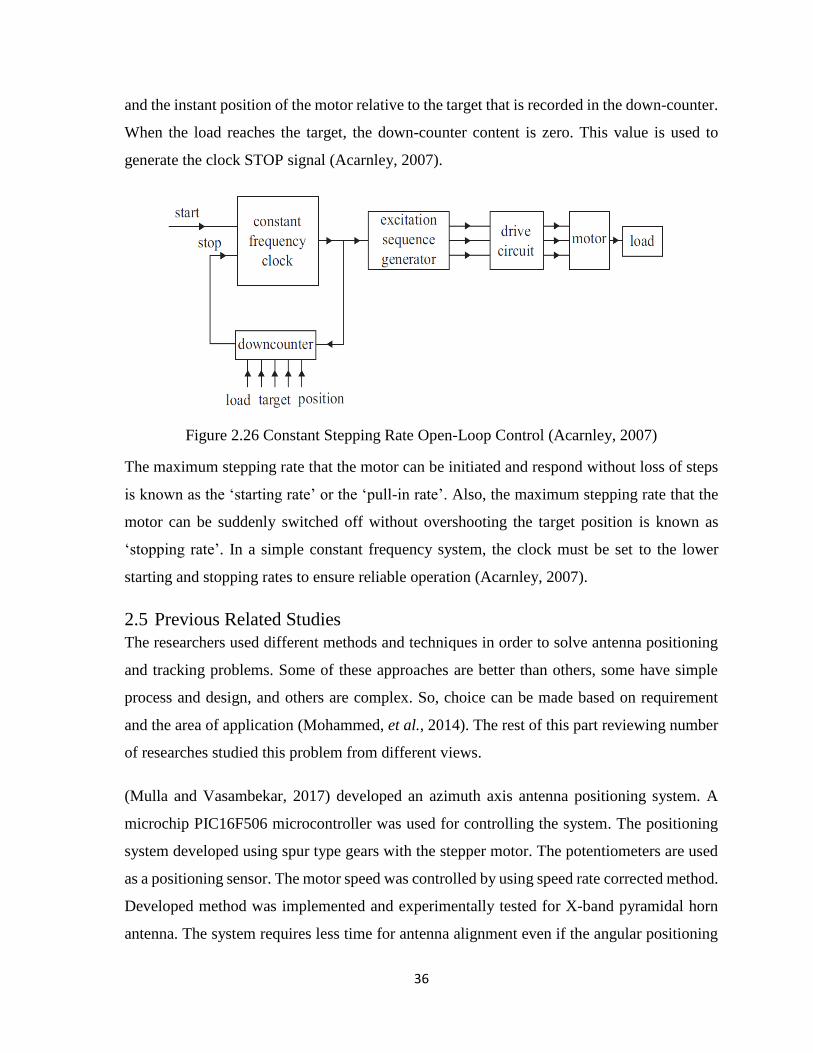
36

and the instant position of the motor relative to the target that is recorded in the down-counter.

When the load reaches the target, the down-counter content is zero. This value is used to

generate the clock STOP signal (Acarnley, 2007).

Figure 2.26 Constant Stepping Rate Open-Loop Control (Acarnley, 2007)

The maximum stepping rate that the motor can be initiated and respond without loss of steps

is known as the ‘starting rate’ or the ‘pull-in rate’. Also, the maximum stepping rate that the

motor can be suddenly switched off without overshooting the target position is known as

‘stopping rate’. In a simple constant frequency system, the clock must be set to the lower

starting and stopping rates to ensure reliable operation (Acarnley, 2007).

2.5 Previous Related Studies

The researchers used different methods and techniques in order to solve antenna positioning

and tracking problems. Some of these approaches are better than others, some have simple

process and design, and others are complex. So, choice can be made based on requirement

and the area of application (Mohammed, et al., 2014). The rest of this part reviewing number

of researches studied this problem from different views.

(Mulla and Vasambekar, 2017) developed an azimuth axis antenna positioning system. A

microchip PIC16F506 microcontroller was used for controlling the system. The positioning

system developed using spur type gears with the stepper motor. The potentiometers are used

as a positioning sensor. The motor speed was controlled by using speed rate corrected method.

Developed method was implemented and experimentally tested for X-band pyramidal horn

antenna. The system requires less time for antenna alignment even if the angular positioning

37

error is large. It is a low cost solution for fast and large antenna alignment for the desired

satellite (Mulla and Vasambekar, 2017).

(Linus Aloo, et al., 2016) addressed antenna positioning control system that was based on DC

servomotor. The design was simulated in MATLAB/SIMULINK software. The research aims

to minimize the deviations from the desired position. Proportional-integral-derivative (PID)

controller was used in the first test. The obtained results of the tuned PID controller were

improved by adding linear quadratic regulator (LQR) which apart from optimizing the system

response increases the accuracy of the state variables by estimating the states. The results

show that the performance of the hybrid PID-LQR controller is much better than that of the

PID controller in terms of reduced settling time and overshoot (Linus Aloo, et al., 2016).

(Prajwal, et al., 2015) proposed system helps in adjusting the dish antenna position remotely

by using smart-phone/tablet operating android application program. The smart-phone/tablet

acts as a transmitter which sends data to Arduino microcontroller via Bluetooth device. The

micro-controller manages motor motion by sending control signals to the motors-drivers. The

proposed system controls the dish rotation in two axes (X and Y). System measurements were

carried out using the fully functional but not optimal device built on the breadboard (Prajwal,

et al., 2015).

(Rajini and Murthy, 2015) discussed an antenna servo control system for remote sensing

satellite ground station. The mathematical model of servo control system was presented. A

close loop system using PID controller was demonstrated. System stability conditions were

verified. The performance of the system increases by implementing a fuzzy controller.

(Abdul Rehman, et al., 2014) studied the design and implementation of azimuth antenna

position control system. The response of the system without using any controller was studied

and noticed that the response was not good. For getting a better response, a PID controller has

been used. Then LQR controller was added to the deigned system so as to get better response

in case of disturbance. The study illustrates that the LQR results are much better than the

results obtained by PID controller (Abdul Rehman, et al., 2014).

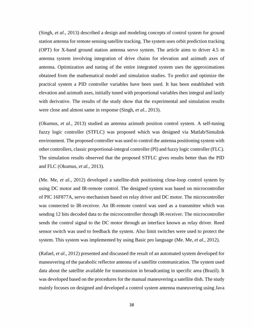
38

(Singh, et al., 2013) described a design and modeling concepts of control system for ground

station antenna for remote sensing satellite tracking. The system uses orbit prediction tracking

(OPT) for X-band ground station antenna servo system. The article aims to driver 4.5 m

antenna system involving integration of drive chains for elevation and azimuth axes of

antenna. Optimization and tuning of the entire integrated system uses the approximations

obtained from the mathematical model and simulation studies. To predict and optimize the

practical system a PID controller variables have been used. It has been established with

elevation and azimuth axes, initially tuned with proportional variables then integral and lastly

with derivative. The results of the study show that the experimental and simulation results

were close and almost same in response (Singh, et al., 2013).

(Okumus, et al., 2013) studied an antenna azimuth position control system. A self-tuning

fuzzy logic controller (STFLC) was proposed which was designed via Matlab/Simulink

environment. The proposed controller was used to control the antenna positioning system with

other controllers, classic proportional-integral controller (PI) and fuzzy logic controller (FLC).

The simulation results observed that the proposed STFLC gives results better than the PID

and FLC (Okumus, et al., 2013).

(Me. Me, et al., 2012) developed a satellite-dish positioning close-loop control system by

using DC motor and IR-remote control. The designed system was based on microcontroller

of PIC 16F877A, servo mechanism based on relay driver and DC motor. The microcontroller

was connected to IR-receiver. An IR-remote control was used as a transmitter which was

sending 12 bits decoded data to the microcontroller through IR-receiver. The microcontroller

sends the control signal to the DC motor through an interface known as relay driver. Reed

sensor switch was used to feedback the system. Also limit switches were used to protect the

system. This system was implemented by using Basic pro language (Me. Me, et al., 2012).

(Rafael, et al., 2012) presented and discussed the result of an automated system developed for

maneuvering of the parabolic reflector antenna of a satellite communication. The system used

data about the satellite available for transmission in broadcasting in specific area (Brazil). It

was developed based on the procedures for the manual maneuvering a satellite dish. The study

mainly focuses on designed and developed a control system antenna maneuvering using Java

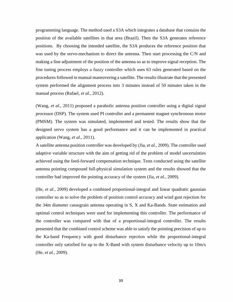
39

programming language. The method used a S3A which integrates a database that contains the

position of the available satellites in that area (Brazil). Then the S3A generates reference

positions. By choosing the intended satellite, the S3A produces the reference position that

was used by the servo-mechanism to direct the antenna. Then start processing the C/N and

making a fine adjustment of the position of the antenna so as to improve signal reception. The

fine tuning process employs a fuzzy controller which uses 63 rules generated based on the

procedures followed in manual maneuvering a satellite. The results illustrate that the presented

system performed the alignment process into 3 minutes instead of 50 minutes taken in the

manual process (Rafael, et al., 2012).

(Wang, et al., 2011) proposed a parabolic antenna position controller using a digital signal

processor (DSP). The system used PI controller and a permanent magnet synchronous motor

(PMSM). The system was simulated, implemented and tested. The results show that the

designed servo system has a good performance and it can be implemented in practical

application (Wang, et al., 2011).

A satellite antenna position controller was developed by (Jia, et al., 2009). The controller used

adaptive variable structure with the aim of getting rid of the problem of model uncertainties

achieved using the feed-forward compensation technique. Tests conducted using the satellite

antenna pointing compound full-physical simulation system and the results showed that the

controller had improved the pointing accuracy of the system (Jia, et al., 2009).

(He, et al., 2009) developed a combined proportional-integral and linear quadratic gaussian

controller so as to solve the problem of position control accuracy and wind gust rejection for

the 34m diameter cassegrain antenna operating in S, X and Ka-Bands. State estimation and

optimal control techniques were used for implementing this controller. The performance of

the controller was compared with that of a proportional-integral controller. The results

presented that the combined control scheme was able to satisfy the pointing precision of up to

the Ka-band Frequency with good disturbance rejection while the proportional-integral

controller only satisfied for up to the X-Band with system disturbance velocity up to 10m/s

(He, et al., 2009).

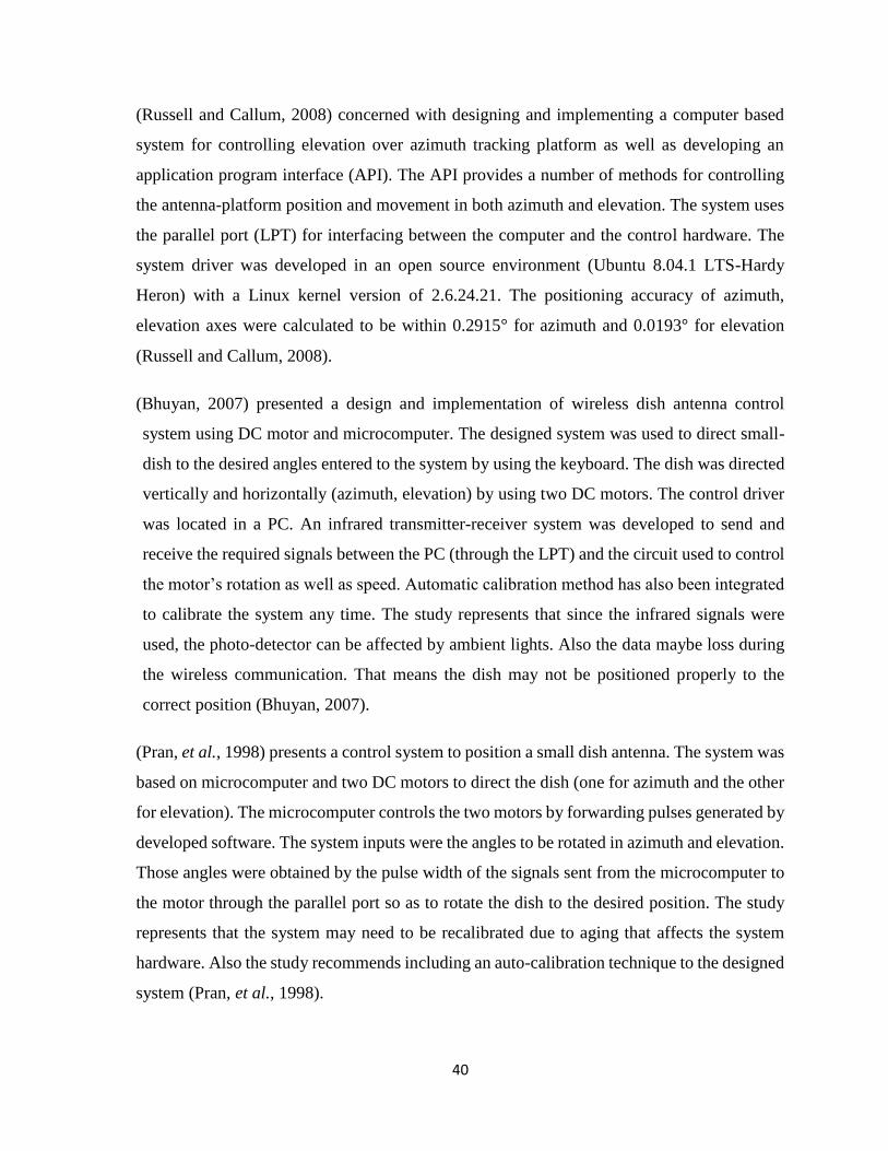
40

(Russell and Callum, 2008) concerned with designing and implementing a computer based

system for controlling elevation over azimuth tracking platform as well as developing an

application program interface (API). The API provides a number of methods for controlling

the antenna-platform position and movement in both azimuth and elevation. The system uses

the parallel port (LPT) for interfacing between the computer and the control hardware. The

system driver was developed in an open source environment (Ubuntu 8.04.1 LTS-Hardy

Heron) with a Linux kernel version of 2.6.24.21. The positioning accuracy of azimuth,

elevation axes were calculated to be within 0.2915° for azimuth and 0.0193° for elevation

(Russell and Callum, 2008).

(Bhuyan, 2007) presented a design and implementation of wireless dish antenna control

system using DC motor and microcomputer. The designed system was used to direct small-

dish to the desired angles entered to the system by using the keyboard. The dish was directed

vertically and horizontally (azimuth, elevation) by using two DC motors. The control driver

was located in a PC. An infrared transmitter-receiver system was developed to send and

receive the required signals between the PC (through the LPT) and the circuit used to control

the motor’s rotation as well as speed. Automatic calibration method has also been integrated

to calibrate the system any time. The study represents that since the infrared signals were

used, the photo-detector can be affected by ambient lights. Also the data maybe loss during

the wireless communication. That means the dish may not be positioned properly to the

correct position (Bhuyan, 2007).

(Pran, et al., 1998) presents a control system to position a small dish antenna. The system was

based on microcomputer and two DC motors to direct the dish (one for azimuth and the other

for elevation). The microcomputer controls the two motors by forwarding pulses generated by

developed software. The system inputs were the angles to be rotated in azimuth and elevation.

Those angles were obtained by the pulse width of the signals sent from the microcomputer to

the motor through the parallel port so as to rotate the dish to the desired position. The study

represents that the system may need to be recalibrated due to aging that affects the system

hardware. Also the study recommends including an auto-calibration technique to the designed

system (Pran, et al., 1998).

41

Table 2.2 summarizes the remarks on the related studies into a number of points and can be

arranged into; design complexity, tuning complications, significant delay in dish-antenna

directing time, using two factors (azimuth/elevation) to direct the antenna and needing more

controller to improve the performance.

In this research the polarization factor is considered and straight open-loop control method is

used to avoid the design complexity, tuning complexity and enhance the dish-antenna

directing time by using new technology.

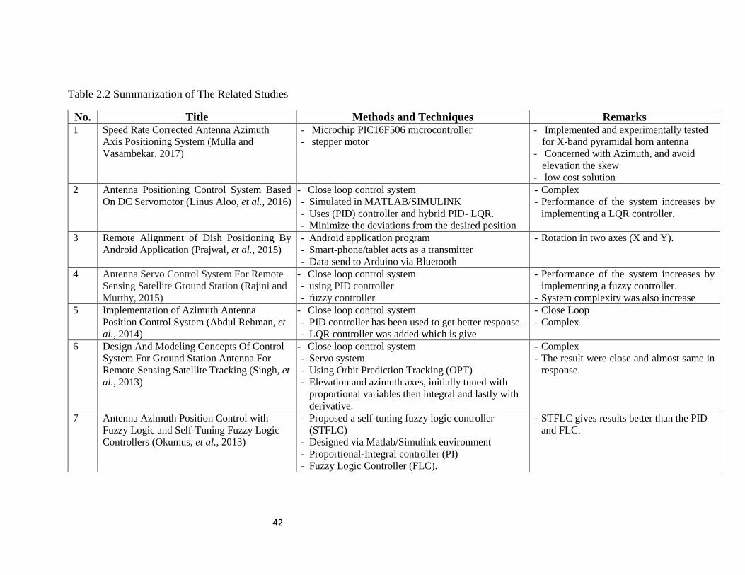
42

Table 2.2 Summarization of The Related Studies

No. Title Methods and Techniques Remarks 1 Speed Rate Corrected Antenna Azimuth

Axis Positioning System (Mulla and

Vasambekar, 2017)

- Microchip PIC16F506 microcontroller

- stepper motor

- Implemented and experimentally tested

for X-band pyramidal horn antenna

- Concerned with Azimuth, and avoid

elevation the skew

- low cost solution

2 Antenna Positioning Control System Based

On DC Servomotor (Linus Aloo, et al., 2016)

- Close loop control system

- Simulated in MATLAB/SIMULINK

- Uses (PID) controller and hybrid PID- LQR.

- Minimize the deviations from the desired position

- Complex

- Performance of the system increases by

implementing a LQR controller.

3 Remote Alignment of Dish Positioning By

Android Application (Prajwal, et al., 2015)

- Android application program

- Smart-phone/tablet acts as a transmitter

- Data send to Arduino via Bluetooth

- Rotation in two axes (X and Y).

4 Antenna Servo Control System For Remote

Sensing Satellite Ground Station (Rajini and

Murthy, 2015)


- using PID controller

- fuzzy controller

- Performance of the system increases by

implementing a fuzzy controller.

- System complexity was also increase

5 Implementation of Azimuth Antenna

Position Control System (Abdul Rehman, et

al., 2014)


- PID controller has been used to get better response.

- LQR controller was added which is give

- Close Loop

- Complex

6 Design And Modeling Concepts Of Control

System For Ground Station Antenna For

Remote Sensing Satellite Tracking (Singh, et

al., 2013)


- Servo system

- Using Orbit Prediction Tracking (OPT)

- Elevation and azimuth axes, initially tuned with

proportional variables then integral and lastly with

derivative.

- Complex

- The result were close and almost same in

response.

7 Antenna Azimuth Position Control with

Fuzzy Logic and Self-Tuning Fuzzy Logic

Controllers (Okumus, et al., 2013)

- Proposed a self-tuning fuzzy logic controller

(STFLC)

- Designed via Matlab/Simulink environment

- Proportional-Integral controller (PI)

- Fuzzy Logic Controller (FLC).

- STFLC gives results better than the PID

and FLC.

43

8 Satellite Dish Positioning Control by DC

Motor Using IR Remote Control (Me. Me, et

al., 2012)


- Based on microcontroller of PIC 16F877A.

- Servo mechanism.

- Relay driver and DC motor

- Concerned with Azimuth, elevation and

avoid the polarization.

9 Development of An Automated System For

Maneuvering Parabolic Dish Antennas Used

In Satellite Comunication (Rafael, et al.,

2012)


- Used fuzzy logic controller

- S3A integrates database containing data about the

satellites available in specific area.

- Fine tuning the dish- antenna within 3

min instead of 50 min in manual process


avoid the polarization

10 The Design and Implementation of the Digital

Servo System for the Satellite Antenna

(Wang, et al., 2011)


- Using a Digital signal Processor (DSP)

- Using PI controller

- Permanent Magnet Synchronous Motor (PMSM)

- Designed servo system has a good

performance.

11 Study of Adaptive Variable Structure

Attitude Control and its full Physical

Simulation of Multi-Body Satellite Antenna

Drive Control (Jia, et al., 2009)

- Close Loop control system

- Using adaptive variable structure

- Complex

- Results showed that the controller had

improved the pointing accuracy of the

system.

12 LQG Controller with Wind Gust Disturbance

Rejection Property for Cassegrain Antenna

(He, et al., 2009)

- developed a combined proportional-integral and

Linear Quadratic Gaussian controller

- Operating in S,X and Ka-Bands

- Results presented that the combine

control scheme was able to satisfy the

pointing precision of up to the Ka- band

Frequency.

13 Designing And Implementing A Computer

Based System For Controlling Elevation Over

Azimuth Tracking (Russell and Callum,

2008)

- developing an Application Program Interface (API)

- uses the Parallel Port (LPT)

- The positioning accuracy of azimuth,

elevation axes were calculated to be

within 0.2915° for azimuth and 0.0193°

for elevation.


avoid the skew.

14 WIRELESS CONTROL SYSTEM FOR DC

MOTOR TO POSITION A DISH

ANTENNA USING MICROCOMPUTER

(Muhibul Haque Bhuyan, 2007)


- Infrared transmitter-receiver system

- DC motors were used to direct the antenna


avoid the skew

- The desired angles were entered to the

system by using the keyboard

15 Microcomputer Based Dish Antenna Position

Control System (Pran, et al., 1998)

- Two DC motors were used to direct the antenna

- LPT port was used to send signal to

- System inputs were azimuth and

elevation angles

- system need to recalibrated

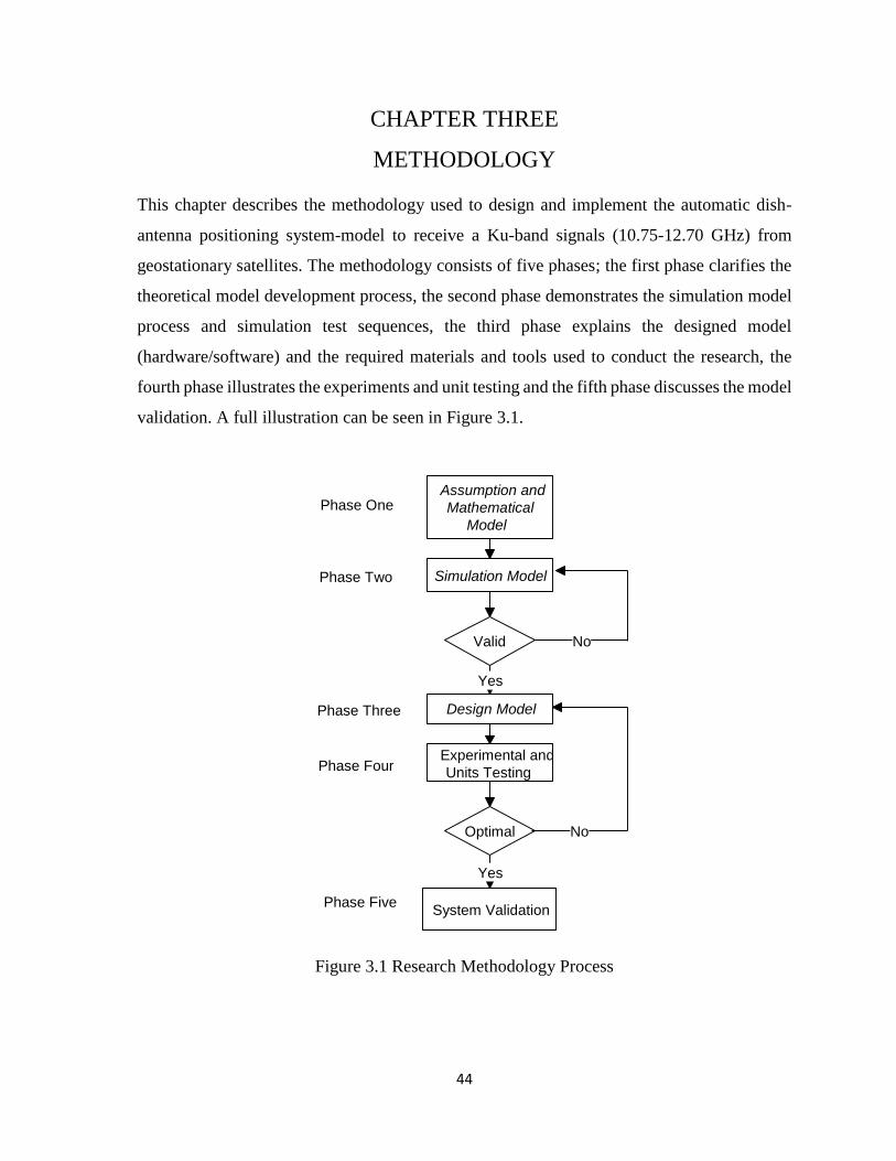
44

CHAPTER THREE

3 METHODOLOGY

This chapter describes the methodology used to design and implement the automatic dish-

antenna positioning system-model to receive a Ku-band signals (10.75-12.70 GHz) from

geostationary satellites. The methodology consists of five phases; the first phase clarifies the

theoretical model development process, the second phase demonstrates the simulation model

process and simulation test sequences, the third phase explains the designed model

(hardware/software) and the required materials and tools used to conduct the research, the

fourth phase illustrates the experiments and unit testing and the fifth phase discusses the model

validation. A full illustration can be seen in Figure 3.1.

Figure 3.1 Research Methodology Process

Assumption and Mathematical

Model

Simulation Model

Design Model

Phase One

Phase Four

System Validation Phase Five

Valid No No

Yes Yes

Phase Two

Phase Three

Optimal No No

Yes Yes

Experimental and Units Testing

45

3.1 Theoretical model development processes

Model design process starts from formulating the design theoretically then transforms the

theoretical into real model. The theoretical part consists of; assumptions, arrangements and

mathematical equations.

3.1.1 Assumptions and Arrangements

The research was based on the following assumptions and arrangements.

Target satellites:

o Geostationary satellites that transmit signals in Ku-band range (10.75-12.70

GHz).

o Satellites that the antenna-site was located on its coverage area (foot-print).

The used antenna: 60 cm dish-antenna that has an HPBW up to 3° when it was used for

receiving Ku-Band signals.

The proposed system was designed to operate on the northern hemisphere specifically

in Sudan.

The used motors:

o Stepper-motors with step-angles equal to 1.8°.

o Operated in two modes. Half-stepping mode with step-angle 0.9° and micro-

stepping mode with step-angle up-to 0.18°.

3.1.2 Mathematical Model

The mathematical model explains the equations used in the designed system-driver. Also it

explained the drive relationships between system components that limit the design process.

Azimuth and elevation part

For specific site in the northern hemisphere, azimuth and elevation angles can be calculated

based on the below standard equations:

𝑎𝑧𝑐𝑎𝑙 = 180 + 𝑎𝑟𝑐𝑡𝑎𝑛 (𝑡𝑎𝑛(𝐺)

𝑠𝑖𝑛(𝐿))−→ (3.1)

𝑒𝑙𝑐𝑎𝑙 = 𝑎𝑟𝑐𝑡𝑎𝑛 (𝑐𝑜𝑠(𝐺) .𝑐𝑜𝑠(𝐿)−0.1512

√1−𝑐𝑜𝑠2(𝐺).𝑐𝑜𝑠2(𝐿)) −→ (3.2)

46

Where:

𝑎𝑧𝑐𝑎𝑙= azimuth of antenna in degrees

𝑒𝑙𝑐𝑎𝑙=elevation of antenna in degrees

S= sub-satellite point longitude in degrees

N= site longitude in degrees

L= site latitude in degrees

G= S-N

The calculated angles in the above section transformed into a number of steps based on step-

angle of the used stepper-motors. The transformation was done as follows:

𝑎𝑧 =𝑎𝑧𝑐𝑎𝑙𝛽𝑎𝑧

−→ (3.3)

𝑒𝑙 =𝑒𝑙𝑐𝑎𝑙𝛽𝑒𝑙

−→ (3.4)

Where:

𝛽𝑎𝑧 = 𝑆𝑡𝑒𝑝 𝑎𝑛𝑔𝑙𝑒 𝑜𝑓 𝑡ℎ𝑒 𝑎𝑧𝑖𝑚𝑢𝑡ℎ 𝑚𝑜𝑡𝑜𝑟

𝛽𝑒𝑙 = 𝑆𝑡𝑒𝑝 𝑎𝑛𝑔𝑙𝑒 𝑜𝑓 𝑡ℎ𝑒 𝑒𝑙𝑒𝑣𝑎𝑡𝑖𝑜𝑛 𝑚𝑜𝑡𝑜𝑟

The stepping-motor does not offer all calculated positions. It divides the looking radius into

discrete positions based on the step-angle. So, the calculated values in the above equations

(az, and el) maybe integer number (aligned with a discrete position) or float (contents fraction)

that means, it placed between two discrete positions. For all cases, the calculated look-angle

(azimuth, elevation) will drop within four integer cross-points as illustreated in Figure 3.2. So

the optimum choice will be the nearest cross point to the look-angle ( the nearest point to the

center of the main-lobe).

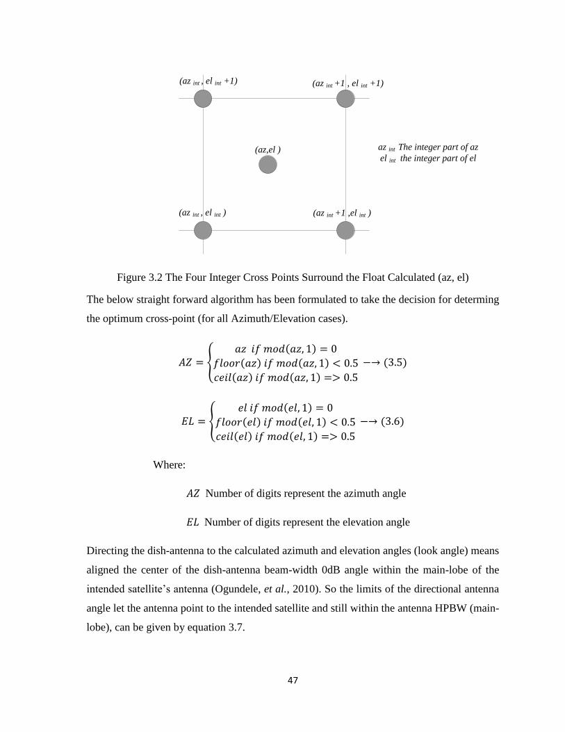
47

(az int +1 ,el int )

(az int , el int +1)

(az int , el int )

(az int +1 , el int +1)

(az,el ) az int The integer part of az

el int the integer part of el

Figure 3.2 The Four Integer Cross Points Surround the Float Calculated (az, el)

The below straight forward algorithm has been formulated to take the decision for determing

the optimum cross-point (for all Azimuth/Elevation cases).

𝐴𝑍 = 𝑎𝑧 𝑖𝑓 𝑚𝑜𝑑(𝑎𝑧, 1) = 0

𝑓𝑙𝑜𝑜𝑟(𝑎𝑧) 𝑖𝑓 𝑚𝑜𝑑(𝑎𝑧, 1) < 0.5

𝑐𝑒𝑖𝑙(𝑎𝑧) 𝑖𝑓 𝑚𝑜𝑑(𝑎𝑧, 1) => 0.5

−→ (3.5)

𝐸𝐿 = 𝑒𝑙 𝑖𝑓 𝑚𝑜𝑑(𝑒𝑙, 1) = 0

𝑓𝑙𝑜𝑜𝑟(𝑒𝑙) 𝑖𝑓 𝑚𝑜𝑑(𝑒𝑙, 1) < 0.5

𝑐𝑒𝑖𝑙(𝑒𝑙) 𝑖𝑓 𝑚𝑜𝑑(𝑒𝑙, 1) => 0.5

−→ (3.6)

Where:

𝐴𝑍 Number of digits represent the azimuth angle

𝐸𝐿 Number of digits represent the elevation angle

Directing the dish-antenna to the calculated azimuth and elevation angles (look angle) means

aligned the center of the dish-antenna beam-width 0dB angle within the main-lobe of the

intended satellite’s antenna (Ogundele, et al., 2010). So the limits of the directional antenna

angle let the antenna point to the intended satellite and still within the antenna HPBW (main-

lobe), can be given by equation 3.7.

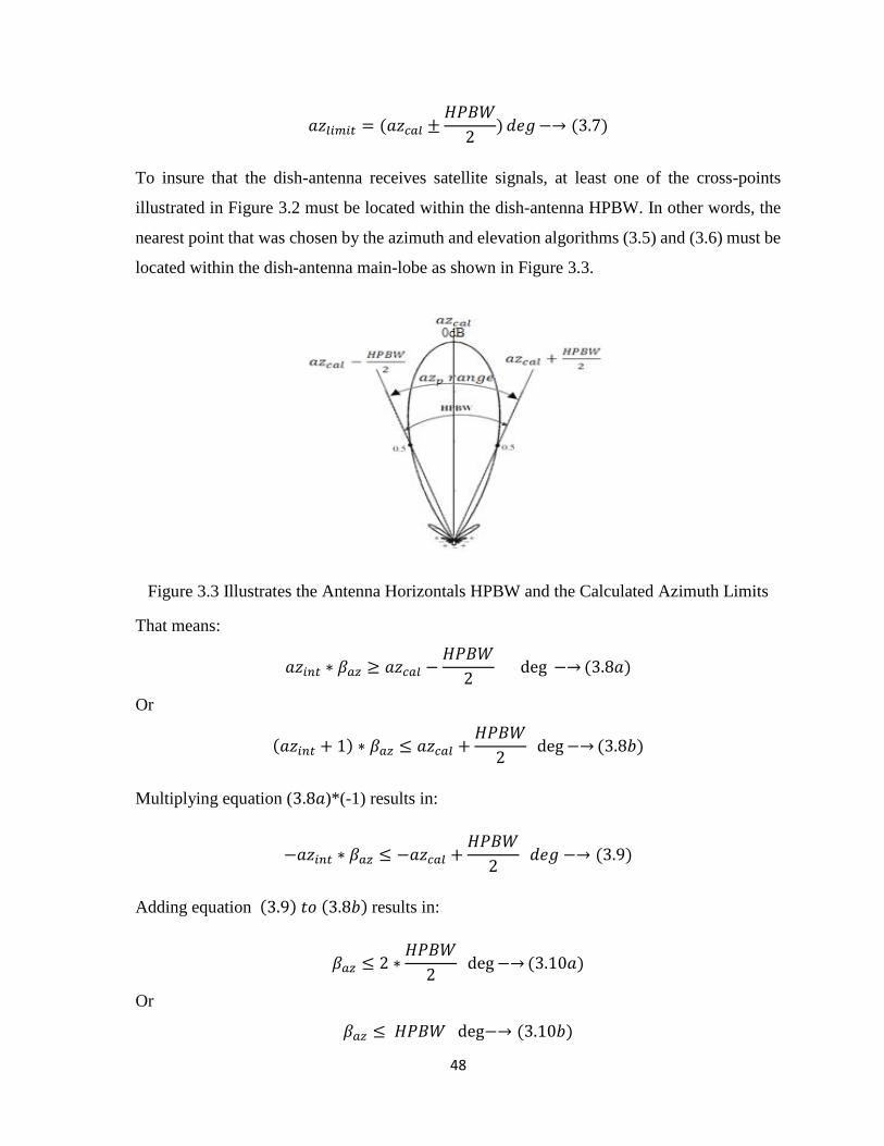
48

𝑎𝑧𝑙𝑖𝑚𝑖𝑡 = (𝑎𝑧𝑐𝑎𝑙 ±𝐻𝑃𝐵𝑊

2)𝑑𝑒𝑔−→ (3.7)

To insure that the dish-antenna receives satellite signals, at least one of the cross-points

illustrated in Figure 3.2 must be located within the dish-antenna HPBW. In other words, the

nearest point that was chosen by the azimuth and elevation algorithms (3.5) and (3.6) must be

located within the dish-antenna main-lobe as shown in Figure 3.3.

Figure 3.3 Illustrates the Antenna Horizontals HPBW and the Calculated Azimuth Limits

That means:

𝑎𝑧𝑖𝑛𝑡 ∗ 𝛽𝑎𝑧 ≥ 𝑎𝑧𝑐𝑎𝑙 −𝐻𝑃𝐵𝑊

2 deg −→(3.8𝑎)

Or

(𝑎𝑧𝑖𝑛𝑡 + 1) ∗ 𝛽𝑎𝑧 ≤ 𝑎𝑧𝑐𝑎𝑙 +𝐻𝑃𝐵𝑊

2 deg−→(3.8𝑏)

Multiplying equation (3.8𝑎)*(-1) results in:

−𝑎𝑧𝑖𝑛𝑡 ∗ 𝛽𝑎𝑧 ≤ −𝑎𝑧𝑐𝑎𝑙 +𝐻𝑃𝐵𝑊

2 𝑑𝑒𝑔 −→ (3.9)

Adding equation (3.9) 𝑡𝑜 (3.8𝑏) results in:

𝛽𝑎𝑧 ≤ 2 ∗𝐻𝑃𝐵𝑊

2 deg−→(3.10𝑎)

Or

𝛽𝑎𝑧 ≤ 𝐻𝑃𝐵𝑊 deg−→ (3.10𝑏)

49

In this study, the used parabolic antenna had elliptical aperture. The HPBW in the horizontal

and vertical were around or equal. So the limitations administrate antenna HPBW and motor

step-angle in the horizontal axis (azimuth) can be generalized also in vertical (elevation). That

means:

𝛽𝑒𝑙 ≤ 𝐻𝑃𝐵𝑊 deg−→ (3.11)

The above azimuth/elevation calculations were the basic that the designed system uses to

position the antenna to the intended satellite in an accurate way.

Polarization Part

In linear polarization (Vertical and Horizontal) used in this research (Ku-band), the LNB must

be aligned with the polarization of the source signal (satellite signal). So the below

polarization angle calculations must be taken in account.

𝑝𝑜𝑙𝑐𝑎𝑙 = 𝑎𝑟𝑐𝑡𝑎𝑛 (𝑠𝑖𝑛(𝐺)

𝑡𝑎𝑛(𝐿))−→ (3.12)

Where:

𝑝𝑜𝑙𝑐𝑎𝑙= polarization angle (skew angle) of the earth-station antenna

G= S-N

S= sub-satellite point longitude in degrees

N= site longitude in degrees

L= site latitude in degrees

Same as followed in azimuth and elevation angles, the calculated polarization-angle must be

changed into a number of steps based on the step-angle of the used stepper-motor:

𝑝𝑜𝑙 =𝑝𝑜𝑙𝑐𝑎𝑙𝛽𝑝𝑜𝑙

−→ (3.13)

Where:

𝛽𝑝𝑜𝑙 = 𝑆𝑡𝑒𝑝 𝑎𝑛𝑔𝑙𝑒 𝑜𝑓 𝑡ℎ𝑒 𝑝𝑜𝑙𝑎𝑟𝑖𝑧𝑎𝑡𝑖𝑜𝑛 𝑚𝑜𝑡𝑜𝑟

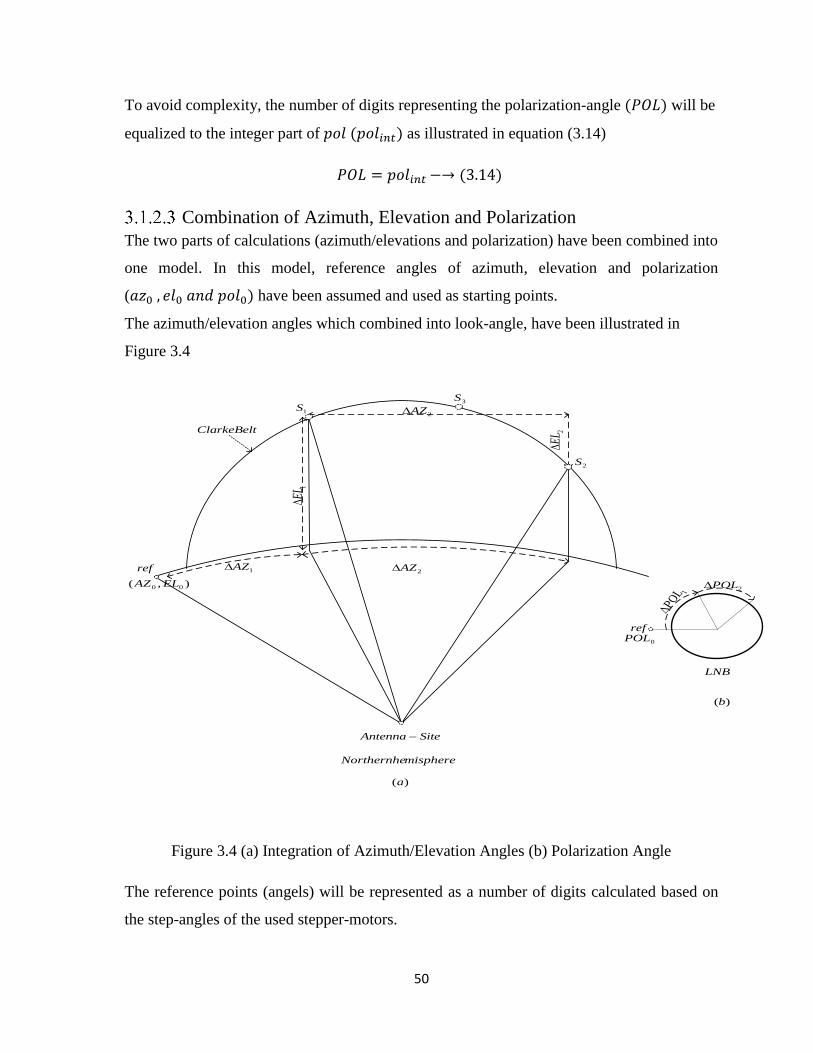
50

To avoid complexity, the number of digits representing the polarization-angle (𝑃𝑂𝐿) will be

equalized to the integer part of 𝑝𝑜𝑙 (𝑝𝑜𝑙𝑖𝑛𝑡) as illustrated in equation (3.14)

𝑃𝑂𝐿 = 𝑝𝑜𝑙𝑖𝑛𝑡 −→ (3.14)

Combination of Azimuth, Elevation and Polarization

The two parts of calculations (azimuth/elevations and polarization) have been combined into

one model. In this model, reference angles of azimuth, elevation and polarization

(𝑎𝑧0 , 𝑒𝑙0 𝑎𝑛𝑑 𝑝𝑜𝑙0) have been assumed and used as starting points.

The azimuth/elevation angles which combined into look-angle, have been illustrated in

Figure 3.4

2AZ1AZ

1EL

2EL

1S

2S

),( 00 ELAZ

ClarkeBelt

SiteAntenna

misphereNorthernhe

1

POL

2POL

LNB

0POL

2AZ

ref

ref

3S

)(a

)(b

Figure 3.4 (a) Integration of Azimuth/Elevation Angles (b) Polarization Angle

The reference points (angels) will be represented as a number of digits calculated based on

the step-angles of the used stepper-motors.

51

𝐴𝑍0 =𝑎𝑧0

𝛽𝑎𝑧⁄ −→ (3.15𝑎)

𝐸𝐿0 =𝑒𝑙0

𝛽𝑒𝑙⁄ −→ (3.15𝑏)

𝑃𝑂𝐿0 =𝑝𝑜𝑙0

𝛽𝑝𝑜𝑙⁄ −→ (3.15𝑐)

Figure 3.4(a), starting from the reference points (𝐴𝑍0 , 𝐸𝐿0𝑎𝑛𝑑 𝑃𝑂𝐿0), to let the dish antenna

point to one of these satellites (assumed S1) which was represented by the digits AZ1, EL1 and

POL1 respectively. The motors must move the difference between azimuth, elevation and

polarization digits of S1 satellite and the reference points. These can be calculated using

equations 3.16a up-to 3.16c.

𝛥𝐴𝑍1 = 𝐴𝑍1 − 𝐴𝑍0−→ (3.16𝑎)

𝛥𝐸𝐿1 = 𝐸𝐿1 − 𝐸𝐿0−→ (3.16𝑏)

𝛥𝑃𝑂𝐿1 = 𝑃𝑂𝐿1 − 𝑃𝑂𝐿0−→ (3.16𝑐)

Also to move the dish-antenna from S1 to S2 that’s illustrated in

Figure 3.4, the motors must move the difference between azimuth, elevation and polarization

digits present S1 and S2. These can be calculated using equations 3.17a up-to 3.17c.

𝛥𝐴𝑍2 = 𝐴𝑍2 − 𝐴𝑍1−→ (3.17𝑎)

𝛥𝐸𝐿2 = 𝐸𝐿2 − 𝐸𝐿1−→ (3.17𝑏)

𝛥𝑃𝑂𝐿2 = 𝑃𝑂𝐿2 − 𝑃𝑂𝐿1−→ (3.17𝑐)

The general form of the above equations for all visible satellites can be formulated as follows:

𝛥𝐴𝑧𝑛 = 𝐴𝑧𝑛 − 𝐴𝑧𝑛−1−→ (3.18𝑎)

𝛥𝐸𝑙𝑛 = 𝐸𝑙𝑛 − 𝐸𝑙𝑛−1−→ (3.18𝑏)

𝛥𝑃𝑜𝑙𝑛 = 𝑃𝑜𝑙𝑛 − 𝑃𝑜𝑙𝑛−1−→ (3.18𝑐)

The negative value of every 𝛥 in the above equations means that the espacific motor

movement is CCW.

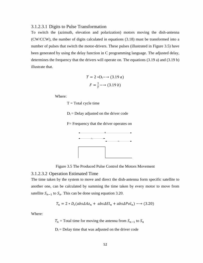
52

3.1.2.3.1 Digits to Pulse Transformation

To switch the (azimuth, elevation and polarization) motors moving the dish-antenna

(CW/CCW), the number of digits calculated in equations (3.18) must be transformed into a

number of pulses that switch the motor-drivers. These pulses (illustrated in Figure 3.5) have

been generated by using the delay function in C programming language. The adjusted delay,

determines the frequency that the drivers will operate on. The equations (3.19 a) and (3.19 b)

illustrate that.

𝑇 = 2 ∗Dt−→ (3.19 𝑎)

𝐹 =1

𝑇−→ (3.19 𝑏)

Where:

T = Total cycle time

Dt = Delay adjusted on the driver code

F= Frequency that the driver operates on

Dt

Dt

T

Figure 3.5 The Produced Pulse Control the Motors Movement

3.1.2.3.2 Operation Estimated Time

The time taken by the system to move and direct the dish-antenna form specific satellite to

another one, can be calculated by summing the time taken by every motor to move from

satellite 𝑆𝑛−1 to 𝑆𝑛. This can be done using equation 3.20.

𝑇𝑛 = 2 ∗ 𝐷𝑡(𝑎𝑏𝑠𝛥𝐴𝑧𝑛 + 𝑎𝑏𝑠𝛥𝐸𝑙𝑛 + 𝑎𝑏𝑠𝛥𝑃𝑜𝑙𝑛) −→ (3.20)

Where:

𝑇𝑛 = Total time for moving the antenna from 𝑆𝑛−1 to 𝑆𝑛

Dt = Delay time that was adjusted on the driver code

53

𝑎𝑏𝑠𝛥𝐴𝑧𝑛= absolute value of the 𝐴𝑧 difference

𝑎𝑏𝑠𝛥𝐸𝑙𝑛= absolute value of the 𝐸𝑙 difference

𝑎𝑏𝑠𝛥𝑃𝑜𝑙𝑛= absolute value of the 𝑃𝑜𝑙 difference

3.1.2.3.3 System Position Precision Calculation

Practically, because of the different error sources, the azimuth/elevation measured angles may

not be equal to the calculated ones. So, the precision of azimuth/elevation readings must be

defined. It will be represented as a gain with mismatching loss which was calculated based on

angles misalignment (difference between the calculated angles and the measure ones).

The azimuth and elevation misalignment angles can be represented as:

∆𝑎𝑧 = 𝑎𝑧𝑐𝑎𝑙 − 𝑎𝑧𝑚 −→ (3.21𝑎)

∆𝑒𝑙 = 𝑒𝑙𝑐𝑎𝑙 − 𝑒𝑙𝑚 −→ (3.21𝑏)

Where:

∆𝑎𝑧 𝑖𝑠 𝑡ℎ𝑒 𝑎𝑧𝑖𝑚𝑢𝑡ℎ 𝑚𝑖𝑠𝑎𝑙𝑖𝑔𝑛𝑚𝑒𝑛𝑡 𝑎𝑛𝑔𝑙𝑒 𝑖𝑛 𝑑𝑒𝑔𝑟𝑒𝑒𝑠

∆𝑒𝑙 𝑖𝑠 𝑡ℎ𝑒 𝑒𝑙𝑒𝑣𝑎𝑡𝑖𝑜𝑛 𝑚𝑖𝑠𝑎𝑙𝑖𝑔𝑛𝑚𝑒𝑛𝑡 𝑎𝑛𝑔𝑙𝑒 𝑖𝑛 𝑑𝑒𝑔𝑟𝑒𝑒𝑠

𝑎𝑧𝑐𝑎𝑙 𝑖𝑠 𝑡ℎ𝑒 𝑐𝑎𝑙𝑐𝑢𝑙𝑎𝑡𝑒𝑑 𝑎𝑧𝑖𝑚𝑢𝑡ℎ 𝑖𝑛 𝑑𝑒𝑔𝑟𝑒𝑒𝑠

𝑒𝑙𝑐𝑎𝑙 𝑖𝑠 𝑡ℎ𝑒 𝑐𝑎𝑙𝑐𝑢𝑙𝑎𝑡𝑒𝑑 𝑒𝑙𝑒𝑣𝑎𝑡𝑖𝑜𝑛 𝑖𝑛 𝑑𝑒𝑔𝑟𝑒𝑒𝑠

𝑎𝑧𝑚 𝑖𝑠 𝑡ℎ𝑒 𝑚𝑎𝑒𝑠𝑢𝑟𝑒𝑑 𝑎𝑧𝑖𝑚𝑢𝑡ℎ 𝑖𝑛 𝑑𝑒𝑔𝑟𝑒𝑒𝑠

𝑒𝑙𝑚 𝑖𝑠 𝑡ℎ𝑒 𝑚𝑎𝑒𝑠𝑢𝑟𝑒𝑑 𝑒𝑙𝑒𝑣𝑎𝑡𝑖𝑜𝑛 𝑖𝑛 𝑑𝑒𝑔𝑟𝑒𝑒𝑠

The absolute value of misalignment angle as a ratio of HPBW can be represented as:

∆𝑎𝑧𝐻𝑃𝐵𝑊 = [(𝑎𝑧𝑐𝑎𝑙 − 𝑎𝑧𝑚)

𝐻𝑃𝐵𝑊𝑎𝑧⁄ ] −→ (3.22𝑎)

∆𝑒𝑙𝐻𝑃𝐵𝑊 = [(𝑒𝑙𝑐𝑎𝑙 − 𝑒𝑙𝑚)

𝐻𝑃𝐵𝑊𝑒𝑙⁄ ] −→ (3.22𝑏)

Where:

∆𝑎𝑧𝐻𝑃𝐵𝑊 𝑖𝑠 𝑡ℎ𝑒 𝑎𝑧𝑖𝑚𝑢𝑡ℎ 𝑚𝑖𝑠𝑎𝑙𝑖𝑔𝑛𝑚𝑒𝑛𝑡 𝑎𝑠 𝑎𝑟𝑡𝑖𝑜 𝑜𝑓 𝐻𝑃𝐵𝑊

∆𝑒𝑙𝐻𝑃𝐵𝑊 𝑖𝑠 𝑡ℎ𝑒 𝑒𝑙𝑒𝑣𝑎𝑡𝑖𝑜𝑛 𝑚𝑖𝑠𝑎𝑙𝑖𝑔𝑛𝑚𝑒𝑛𝑡 𝑎𝑠 𝑎𝑟𝑡𝑖𝑜 𝑜𝑓 𝐻𝑃𝐵𝑊

54

The highest gain (0dB) of the antenna can be obtained when the difference between the

calculated angle and the measured one was equal to zero. Also the half power gain (3dB) that

can be received by the antenna can be obtained when absolute value of ∆𝑎𝑧𝐻𝑃𝐵𝑊 and ∆𝑒𝑙𝐻𝑃𝐵𝑊

were equal to 0.5. The above cases can be represented mathematically as follow:

𝐺𝑎𝑧

= 0(𝑑𝐵) 𝑤ℎ𝑒𝑛 𝑎𝑏𝑠 (∆𝑎𝑧 𝐻𝑃𝐵𝑊𝑎𝑧

⁄ ) = 0

≥ −3(𝑑𝐵) 𝑤ℎ𝑒𝑛 𝑎𝑏𝑠 (∆𝑎𝑧 𝐻𝑃𝐵𝑊𝑎𝑧⁄ ) ≤ 0.5

< −3(𝑑𝐵) 𝑤ℎ𝑒𝑛 𝑎𝑏𝑠 (∆𝑎𝑧 𝐻𝑃𝐵𝑊𝑎𝑧⁄ ) > 0.5

−→ (3.23𝑎)

𝐺𝑒𝑙

= 0(𝑑𝐵) 𝑤ℎ𝑒𝑛 𝑎𝑏𝑠 (∆𝑒𝑙 𝐻𝑃𝐵𝑊𝑒𝑙

⁄ ) = 0

=> −3(𝑑𝐵) 𝑤ℎ𝑒𝑛 𝑎𝑏𝑠 (∆𝑒𝑙 𝐻𝑃𝐵𝑊𝑒𝑙⁄ ) ≤ 0.5

< −3(𝑑𝐵) 𝑤ℎ𝑒𝑛 𝑎𝑏𝑠 (∆𝑒𝑙 𝐻𝑃𝐵𝑊𝑒𝑙⁄ ) > 0.5

−→ (3.23𝑏)

In general, the more the absolute value of misalignment was increased the gain loss increased

and vice-versa. And the more HPBW increased the gain-loss decreased and vice-versa. This

can be calculated using the equations 3.24a and 3.24b.

𝐺𝑎𝑧 = 10 log [1 − 𝑎𝑏𝑠 (∆𝑎𝑧

𝐻𝑃𝐵𝑊𝑎𝑧⁄ )] [𝑑𝐵] −→ (3.24𝑎)

𝐺𝑒𝑙 = 10 log [1 − 𝑎𝑏𝑠 (∆𝑒𝑙

𝐻𝑃𝐵𝑊𝑒𝑙⁄ )] [𝑑𝐵] −→ (3.24𝑏)

The polarization gain with mismatching loss can be calculated using equation (3.24c).

𝐺𝑝𝑜𝑙 = 20 log[cos(𝛽𝑝𝑜𝑙)] [𝑑𝐵] −→ (3.24𝑐)

The gain average of azimuth, elevation and polarization can be obtained by using the

following equations:

𝐴𝑣𝑔 𝐺𝑎𝑧 =∑𝐺𝑎𝑧

𝑛⁄∞

𝑛=1

[𝑑𝐵]−→ (3.25 𝑎)

𝐴𝑣𝑔 𝐺𝑒𝑙 =∑𝐺𝑒𝑙

𝑛⁄∞

𝑛=1

[𝑑𝐵]−→ (3.25 𝑏)

𝐴𝑣𝑔 𝐺𝑝𝑜𝑙 =∑𝐺𝑝𝑜𝑙

𝑛⁄10

𝑛=1

[𝑑𝐵]−→ (3.25 𝑐)

Where: 𝑛 is number of reading

55

The driven equations in the mathematical part would be the base that the system model and

simulation will be based on.

3.2 Simulation Model

This part of research is concerned with simulating the model input, process and output stages.

To achieve that, a C programming code has been developed. The developed code follows the

sequences followed in manual positioning process controlled by the equations derived in the

mathematical model. In this simulation, the computer key-board was used as an input unit and

also used for confirming the operations. The output and important information were monitored

as numerical results that have been used in the system analyses and evaluation. The developed

simulation code follows the below algorithm and flowchart illustrated in Figure 3.6.

step 01: Start.

step 02: Read the antenna instant direction (azimuth, elevation and polarization) which

was saved as a number of pulses or (digits) based on stepper motors step angles.

step 03: Enter Antenna latitude,longitude and intend satellite longitude (degree).

step 04: Calculate the intend satellite azimuth,elevation and polarization (degree).

step 05: Check if the selected satellite is visible (Yes) , continue step 6,7 and so on. Else

(No), stop the procedures and go to the End.

step 06: Confirm the operation. If the decision is (Yes), follow step 7,8 and so on. Else

(No), stop the procedures and go to the End.

step 07: Change the (azimuth,elevation and polarization) calculated in step-4 from degrees

to number of pulses (digits) based on stepper motors step angles.

step 08: Store the values of the last confirmed antenna (azimuth elevation and

polarization) in the antenna data file (which was calculated in step-7).

step 09: Calculate the differences of (azimuths,elevations and polarizations) in step-2 and

step-7 (differences in pulses).

step 10: Move the dish horizintaly (azimuths pulses difference which was obtained in step-

9) until it points to the intended azimuth which was calculated in step-4.

step 11: Move the dish verticaly (elevations pulses difference which was obtained in step-

9) until it points to the intended elevation which was calculated in step-4.

step 12: Change the antenna skew to the new direction (polarizations pulses difference

which was obtained in step-9).

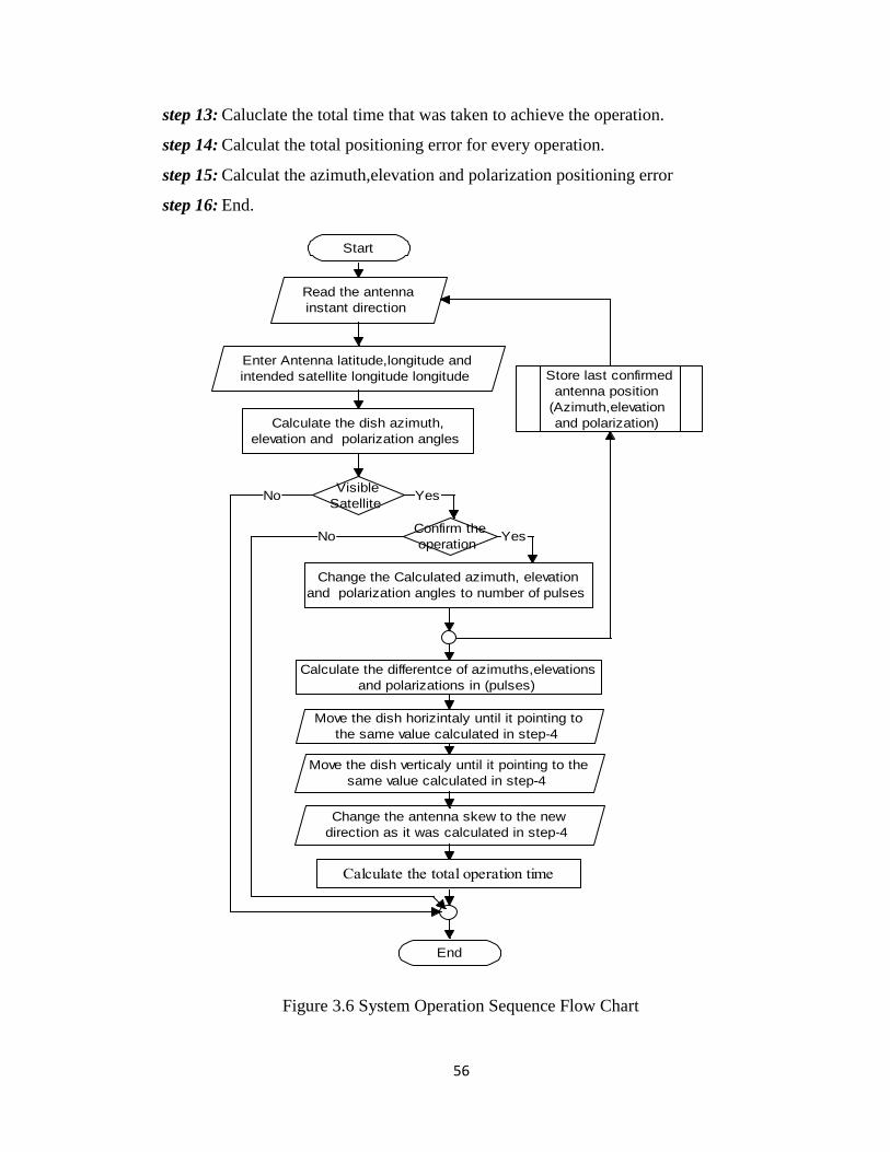
56

Start

End

Enter Antenna latitude,longitude and

intended satellite longitude longitude

Read the antenna

instant direction

Calculate the dish azimuth,

elevation and polarization angles

Visible

Satellite

Confirm the

operation

Change the Calculated azimuth, elevation

and polarization angles to number of pulses

Move the dish horizintaly until it pointing to

the same value calculated in step-4

Move the dish verticaly until it pointing to the

same value calculated in step-4

Change the antenna skew to the new

direction as it was calculated in step-4

Calculate the differentce of azimuths,elevations

and polarizations in (pulses)

Store last confirmed

antenna position

(Azimuth,elevation

and polarization)

NoNo

YesYes

YesYes

NoNo

Calculate the total operation time

Figure 3.6 System Operation Sequence Flow Chart

step 13: Caluclate the total time that was taken to achieve the operation.

step 14: Calculat the total positioning error for every operation.

step 15: Calculat the azimuth,elevation and polarization positioning error

step 16: End.

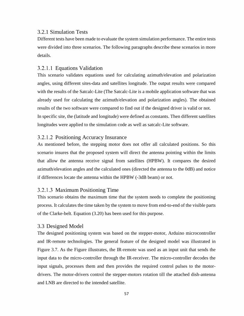
57

3.2.1 Simulation Tests

Different tests have been made to evaluate the system simulation performance. The entire tests

were divided into three scenarios. The following paragraphs describe these scenarios in more

details.

Equations Validation

This scenario validates equations used for calculating azimuth/elevation and polarization

angles, using different sites-data and satellites longitude. The output results were compared

with the results of the Satcalc-Lite (The Satcalc-Lite is a mobile application software that was

already used for calculating the azimuth/elevation and polarization angles). The obtained

results of the two software were compared to find out if the designed driver is valid or not.

In specific site, the (latitude and longitude) were defined as constants. Then different satellites

longitudes were applied to the simulation code as well as satcalc-Lite software.

Positioning Accuracy Insurance

As mentioned before, the stepping motor does not offer all calculated positions. So this

scenario insures that the proposed system will direct the antenna pointing within the limits

that allow the antenna receive signal from satellites (HPBW). It compares the desired

azimuth/elevation angles and the calculated ones (directed the antenna to the 0dB) and notice

if differences locate the antenna within the HPBW (-3dB beam) or not.

Maximum Positioning Time

This scenario obtains the maximum time that the system needs to complete the positioning

process. It calculates the time taken by the system to move from end-to-end of the visible parts

of the Clarke-belt. Equation (3.20) has been used for this purpose.

3.3 Designed Model

The designed positioning system was based on the stepper-motor, Arduino microcontroller

and IR-remote technologies. The general feature of the designed model was illustrated in

Figure 3.7. As the Figure illustrates, the IR-remote was used as an input unit that sends the

input data to the micro-controller through the IR-receiver. The micro-controller decodes the

input signals, processes them and then provides the required control pulses to the motor-

drivers. The motor-drivers control the stepper-motors rotation till the attached dish-antenna

and LNB are directed to the intended satellite.

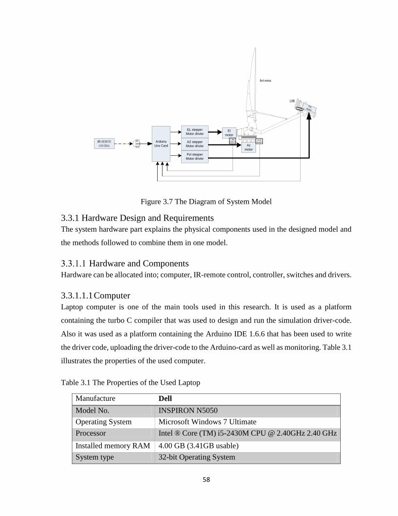
58

Ardoinu

Uno Card

IR-REMOTE CONTROL

El

motor

Antenna

IR-

sen

sor

AZ stepper

Motor drivier

Pol stepper

Motor drivier

EL stepper

Motor drivier

Az

motor

LNB

Polmotor

Limit switch

Limit switch

Limit switch

Figure 3.7 The Diagram of System Model

3.3.1 Hardware Design and Requirements

The system hardware part explains the physical components used in the designed model and

the methods followed to combine them in one model.

Hardware and Components

Hardware can be allocated into; computer, IR-remote control, controller, switches and drivers.

3.3.1.1.1 Computer

Laptop computer is one of the main tools used in this research. It is used as a platform

containing the turbo C compiler that was used to design and run the simulation driver-code.

Also it was used as a platform containing the Arduino IDE 1.6.6 that has been used to write

the driver code, uploading the driver-code to the Arduino-card as well as monitoring. Table 3.1

illustrates the properties of the used computer.

Table 3.1 The Properties of the Used Laptop

Manufacture Dell

Model No. INSPIRON N5050

Operating System Microsoft Windows 7 Ultimate

Processor Intel ® Core (TM) i5-2430M CPU @ 2.40GHz 2.40 GHz

Installed memory RAM 4.00 GB (3.41GB usable)

System type 32-bit Operating System

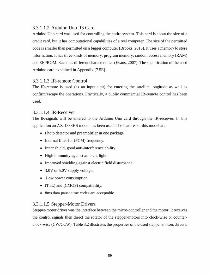
59

3.3.1.1.2 Arduino Uno R3 Card

Arduino Uno card was used for controlling the entire system. This card is about the size of a

credit card, but it has computational capabilities of a real computer. The size of the permitted

code is smaller than permitted on a bigger computer (Brooks, 2015). It uses a memory to store

information. It has three kinds of memory: program memory, random access memory (RAM)

and EEPROM. Each has different characteristics (Evans, 2007). The specification of the used

Arduino card explained in Appendix [7.5E].

3.3.1.1.3 IR-remote Control

The IR-remote is used (as an input unit) for entering the satellite longitude as well as

confirm/escape the operations. Practically, a public commercial IR-remote control has been

used.

3.3.1.1.4 IR-Receiver

The IR-signals will be entered to the Arduino Uno card through the IR-receiver. In this

application an AX-1838HS model has been used. The features of this model are:

Photo detector and preamplifier in one package.

Internal filter for (PCM) frequency.

Inner shield, good anti-interference ability.

High immunity against ambient light.

Improved shielding against electric field disturbance

3.0V or 5.0V supply voltage.

Low power consumption.

(TTL) and (CMOS) compatibility.

8ms data pause time codes are acceptable.

3.3.1.1.5 Stepper-Motor Drivers

Stepper-motor driver was the interface between the micro-controller and the motor. It receives

the control signals then direct the rotator of the stepper-motors into clock-wise or counter-

clock-wise (CW/CCW). Table 3.2 illustrates the properties of the used stepper-motors drivers.

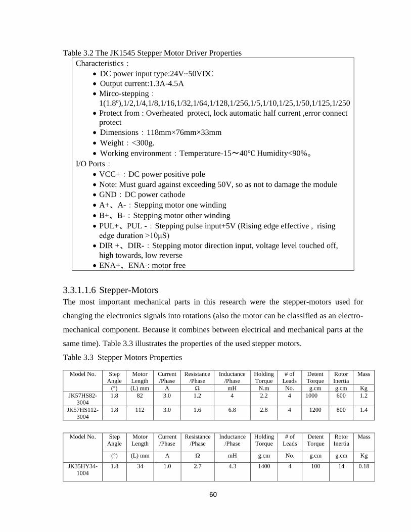
60

Table 3.2 The JK1545 Stepper Motor Driver Properties

Characteristics：

DC power input type:24V~50VDC

Output current:1.3A-4.5A

Mirco-stepping：1(1.8º),1/2,1/4,1/8,1/16,1/32,1/64,1/128,1/256,1/5,1/10,1/25,1/50,1/125,1/250

Protect from : Overheated protect, lock automatic half current ,error connect

protect

Dimensions：118mm×76mm×33mm

Weight：<300g.

Working environment：Temperature-15～40 Humidity<90%。

I/O Ports：

VCC+：DC power positive pole

Note: Must guard against exceeding 50V, so as not to damage the module

GND：DC power cathode

A+、A-：Stepping motor one winding

B+、B-：Stepping motor other winding

PUL+、PUL -：Stepping pulse input+5V (Rising edge effective , rising

edge duration >10μS)

DIR +、DIR-：Stepping motor direction input, voltage level touched off,

high towards, low reverse

ENA+、ENA-: motor free

3.3.1.1.6 Stepper-Motors

The most important mechanical parts in this research were the stepper-motors used for

changing the electronics signals into rotations (also the motor can be classified as an electro-

mechanical component. Because it combines between electrical and mechanical parts at the

same time). Table 3.3 illustrates the properties of the used stepper motors.

Table 3.3 Stepper Motors Properties

Model No. Step

Angle

Motor

Length

Current

/Phase

Resistance

/Phase

Inductance

/Phase

Holding

Torque

# of

Leads

Detent

Torque

Rotor

Inertia

Mass

(°) (L) mm A Ω mH N.m No. g.cm g.cm Kg

JK57HS82-

3004

1.8 82 3.0 1.2 4 2.2 4 1000 600 1.2

JK57HS112-

3004

1.8 112 3.0 1.6 6.8 2.8 4 1200 800 1.4

Model No. Step

Angle

Motor

Length

Current

/Phase

Resistance

/Phase

Inductance

/Phase

Holding

Torque

# of

Leads

Detent

Torque

Rotor

Inertia

Mass

(°) (L) mm A Ω mH g.cm No. g.cm g.cm Kg

JK35HY34-

1004

1.8 34 1.0 2.7 4.3 1400 4 100 14 0.18

61

3.3.1.1.7 Limit Switches

Limit switches have been used to determine the reference points. By pressing every one of

these switches, a logic signal has been sent to the controller changing the status and indicating

that the motor had reached the reference point (explained in more details later).

Entire System Wiring

This part describes the method that was followed to connect the system hardware (stepper

motors, motor-drivers, limit switches, IR-receiver, micro-controller and PC) with each other.

Figure 3.8 illustrates the digital I/O pins used to connect the motor-drivers and the limit

switches to the Arduino card. Pin-2 up to pin-7 configured as output pins to send control signal

to the motor-drivers and pin-8 up-to pin-10 configured as an input to receive signals from the

limit-switches. Each one of the motor-drivers was connected to the Arduino card by using

three wires. One, for deliver pulses that move the specific stepper-motor (CW). The second,

for deliver pulses that move the motor (CCW) and the third one for grounding. Practically,

pin-2 and pin-3 were specified for controlling azimuths motor, pin-4 and pin-5 for controlling

elevations one and pin-6 and pin-7 for controlling polarizations one.

The IR-receiver is the input port that receives the intended satellite longitude as well as the

confirmation command and other control commands.

The USB connection was used to upload the designed system-driver to the Arduino card. Also

it is used to monitor the entered satellite longitude, the calculated azimuth, elevation and

polarization angles and other information.

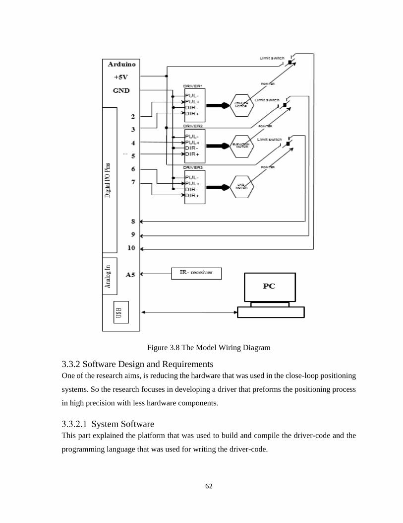
62

Figure 3.8 The Model Wiring Diagram

3.3.2 Software Design and Requirements

One of the research aims, is reducing the hardware that was used in the close-loop positioning

systems. So the research focuses in developing a driver that preforms the positioning process

in high precision with less hardware components.

System Software

This part explained the platform that was used to build and compile the driver-code and the

programming language that was used for writing the driver-code.

63

3.3.2.1.1 Arduino tools

Arduino provided an integrated development environment (IDE) free download from Arduino

website. In this research an Arduino IDE 1.6.6 version was used to develop, compile and

upload the control driver-code to the micro-controller.

3.3.2.1.2 Arduino C

The programming language that was used to write the driver-code was a robust subset of

standard C. This subset of standard C was called Arduino C (Purdum, 2012). Its syntax and

structure are similar to other programming language. So every programmer using any

programming language with experience should have no difficulty in programming the

Arduino, although some hardware-specific language components may be unfamiliar (Brooks,

2015). The major difference between micro controller programming and “conventional”

programming (e.g. uses for scientific and engineering computation) was that the essential

purpose of micro controller programming is to control hardware (Brooks, 2015).

System-Driver Modelling

This part discussed the method that was followed to design the system-driver using Arduino

C language. Every Arduino C code (which is called sketch) consists of setup and loop

functions even if the setup or loop doesn’t do anything. The setup function is executed once

when the Arduino card is turned on, or when the reset-button was pressed (Purdum, 2012).

In this research, the IR-remote control was used to enter the satellite longitude. Also it was

used to control the model with different commands. For different uses of the IR-remote control

and avoiding the complexity, the driver code was written as a multifunction code. Every one

of these functions was called base on demand. This part of the research explained the

algorithms of every function as well as when it was called to serve a specific job.

3.3.2.2.1 Setup function

The setup function is the function that was used to configure the output ports that will be used

to deliver the control signal to the stepper-motor drivers and the input ports that will be used

to receive signals from the IR-remote and limit switches, appendix [A].

64

3.3.2.2.2 Loop function

The loop function was the function that contains the repeatedly run commands. It was used as

the main function in the conventional C code. The other functions have been called from inside

this function based on demand. The Algorithm of this function was explained as follows.

Algorithm:

step 01: Start.

step 02: Receive IR-remote encoded signal.

step 03: Send the received signal to IR-remote Control Decoder function so as to be

decoded.

step 04: If Reset-Sat button was pressed, switch to Reset Satellite function.

step 05: Else, check if the OK button was pressed, switch to Operation Confirm and

Counter Reset functions. Then go to step (8).

step 06: Else check if Exit button was pressed, switch to Counter Reset function. Then

go to step (8).

step 07: Else switch to Satellite Longitude Digits function. Then go to step (8).

step 08: Resume receiving IR-remote input.

step 09: End.

3.3.2.2.3 IR-remote Control Decoder function

The IR-remote was used to input the sub-satellite point (satellite longitude) to the designed

system. This function was used to decode the encoded hexadecimal-numbers which represent

every one of the IR-remote control keys. A special sketch has been used and upload to the

Arduino card to display the encoded hexadecimal number of every one of the IR-remote keys

appendix [7.2B]. The IR-remote number-keys and some of the keys have been used for

execute and confirm commands as mentioned. The remaining keys were decoded to reject or

escape the operation when pressed. This function has been written as a switch statement. It

was formulated as represented in the appendix [7.3C].

3.3.2.2.4 Satellite Longitude Digits Function:

This function was used for entering the IR-decoded numbers used to build the satellite

longitude arranged from 0-360. So the satellite longitude may contains 1 up to 3 digits. The

Arduino Uno starts processing the IR-remote encoded signal as soon as it was received. This

65

function was developed to let the Arduino start the processing after entering the entire digits

of satellite longitude. The function algorithm can be explained as follows:

step 01: Start.

step 02: Press one of the number-keys of the IR-remote (0-9).

step 03: If the number-key pressed value is equal to the longitude of the satellite (for

example 7) then go to step (10). If-else go to the step (4). Else go to step (12).

step 04: Press one of the number-keys for the second time to build the number equal to

the satellite longitude.

step 05: Multiply the first entered number by 10. Then add the second one to the result.

step 06: If the result of the calculations in step (5) is equal to the longitude of the satellite

(for example 23) then go to step (10). If-else go to the next step. Else go to step

(12).

step 07: Press one of the number-keys for the third time to build the number equal to the

satellite longitude.

step 08: Multiply the result of the calculations in step (5) by 10. Then add the third

entered number to the result.

step 09: If the result of the calculations in step (8) is equal to the longitude of the satellite

(for example 334) then go to the next step. Else go to step (12).

step 10: Call Operation Confirm Function to start calculating the azimuth, elevation

and polarization angles.

step 11: If the result of the calculations in step (8) is greater than 360, the system will

escape and back to the starting point.

step 12: Escape the operation.

step 13: End.

Note:

If you press one more digit, the system will erase the entire digits and back to the start

point.

3.3.2.2.5 Operation Confirm Function

This function was called by Loop-function when the operation was confirmed. Also it was

called by Satellite Longitude Digits function. It was used to read the decoded number that

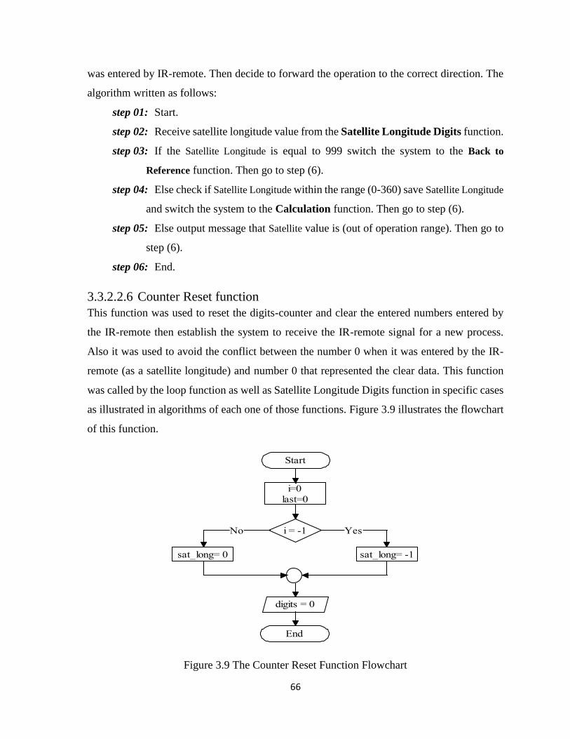
66

was entered by IR-remote. Then decide to forward the operation to the correct direction. The

algorithm written as follows:

step 01: Start.

step 02: Receive satellite longitude value from the Satellite Longitude Digits function.

step 03: If the Satellite Longitude is equal to 999 switch the system to the Back to

Reference function. Then go to step (6).

step 04: Else check if Satellite Longitude within the range (0-360) save Satellite Longitude

and switch the system to the Calculation function. Then go to step (6).

step 05: Else output message that Satellite value is (out of operation range). Then go to

step (6).

step 06: End.

3.3.2.2.6 Counter Reset function

This function was used to reset the digits-counter and clear the entered numbers entered by

the IR-remote then establish the system to receive the IR-remote signal for a new process.

Also it was used to avoid the conflict between the number 0 when it was entered by the IR-

remote (as a satellite longitude) and number 0 that represented the clear data. This function

was called by the loop function as well as Satellite Longitude Digits function in specific cases

as illustrated in algorithms of each one of those functions. Figure 3.9 illustrates the flowchart

of this function.

Figure 3.9 The Counter Reset Function Flowchart

Start

i=0last=0

i = -1

sat_long= -1sat_long= 0

YesYesNoNo

digits = 0

End

67

3.3.2.2.7 Calculations Function

This function contents the equations used to calculate the azimuth/elevation and polarization

angles in degrees then changes it into a number of pulses. Also it generates the pulses and

switches them to the motor-drivers moving the motors and directing the antenna to the

intended satellite.

Practically, the used stepper- motors driver does not response for all operation cases as

expected. Instead of that optimization Algorithm was developed to solve this problem. The

developed optimization algorithm was imbedded in this calculations function appendix [D].

The Calculations function was formulated as the following algorithm and flowchart illustrated

in Figure 3.10.

step 01: Start.

step 02: Receive satellite longitude.

step 03: Read the site latitude, longitude.

step 04: Calculate the azimuth, elevation and polarization angles.

step 05: If the calculated elevation angle is less than 0 (print the selected satellite is

invisible), then go to step 13.

step 06: Else, convert the azimuth, elevation and polarization angles to a number of

pulses.

step 07: Read the last saved antenna azimuth, elevation and polarization number of

pulses.

step 08: Calculate the difference between the azimuths, elevations and polarizations

number of pulses obtained in steps 6 and 7.

step 09: Read the last motors movement directions saved on Arduino RAM.

step 10: Apply the algorithm of optimizing stepper-motor drivers operation appendix

[D].

step 11: Save the last motors movement directions based on calculations in step 8.

step 12: Send the calculated numbers to the specific driver to rotate the motor so as to

direct the antenna to the correct direction.

step 13: End.

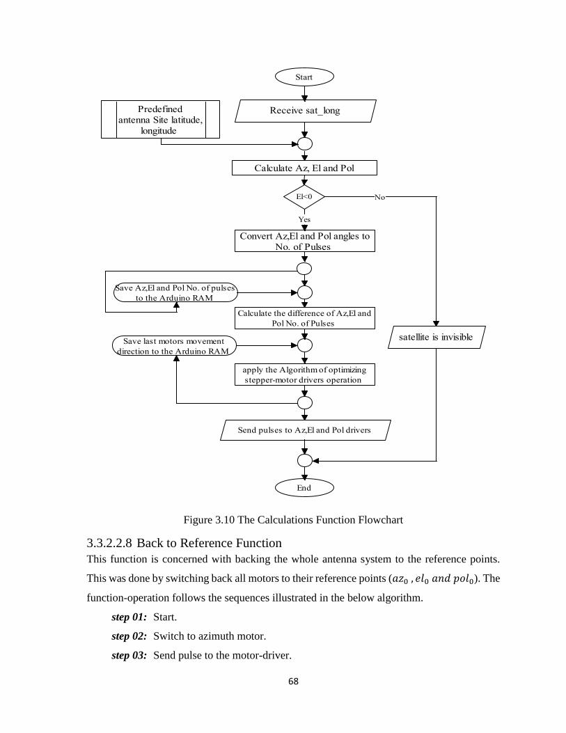
68

Figure 3.10 The Calculations Function Flowchart

3.3.2.2.8 Back to Reference Function

This function is concerned with backing the whole antenna system to the reference points.

This was done by switching back all motors to their reference points (𝑎𝑧0 , 𝑒𝑙0 𝑎𝑛𝑑 𝑝𝑜𝑙0). The

function-operation follows the sequences illustrated in the below algorithm.

step 01: Start.

step 02: Switch to azimuth motor.

step 03: Send pulse to the motor-driver.

End

Predefinedantenna Site latitude,

longitude

Start

Save Az,El and Pol No. of pulses

to the Arduino RAM

Receive sat_long

Calculate Az, El and Pol

El<0 NoNo

Convert Az,El and Pol angles to No. of Pulses

YesYes

Send pulses to Az,El and Pol drivers

Calculate the difference of Az,El and

Pol No. of Pulses

Save last motors movement

direction to the Arduino RAM

apply the Algorithm of optimizing

stepper-motor drivers operation

satellite is invisible

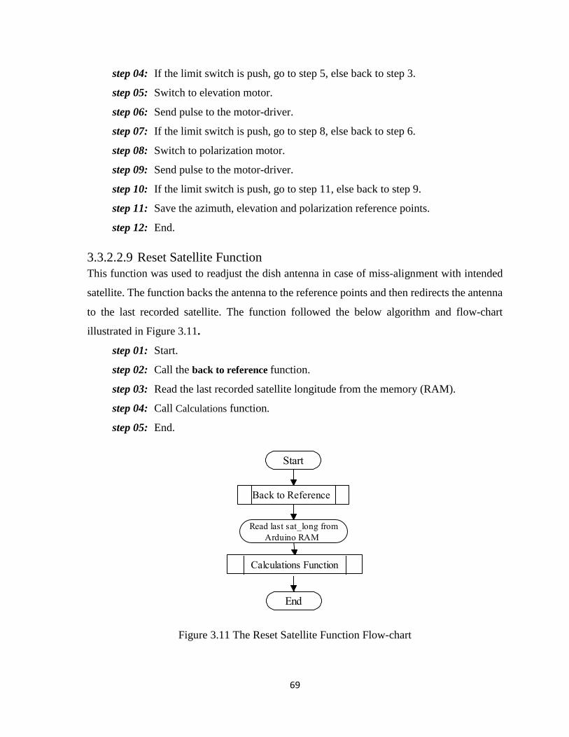
69

step 04: If the limit switch is push, go to step 5, else back to step 3.

step 05: Switch to elevation motor.



step 08: Switch to polarization motor.



step 11: Save the azimuth, elevation and polarization reference points.

step 12: End.

3.3.2.2.9 Reset Satellite Function

This function was used to readjust the dish antenna in case of miss-alignment with intended

satellite. The function backs the antenna to the reference points and then redirects the antenna

to the last recorded satellite. The function followed the below algorithm and flow-chart

illustrated in Figure 3.11.

step 01: Start.

step 02: Call the back to reference function.

step 03: Read the last recorded satellite longitude from the memory (RAM).

step 04: Call Calculations function.

step 05: End.

Figure 3.11 The Reset Satellite Function Flow-chart

Start

End

Read last sat_long from

Arduino RAM

Calculations Function

Back to Reference

70

3.4 Experimental Test

This section explains the methods followed to conduct the research. After completing the

hardware and software design, a number of tests have been done to insure that the designed

system can be implemented in real world.

3.4.1 Unit Testing

It is so complicated to insure that the system components operate in an accurate way if the

system has been tested as one unit. Instead of that, the test was done for every one of stepper-

motors separately.

A protractor has been attached to every one of the motors. Also pointers were fixed to the

rotators of the motors. Different satellites longitudes were applied to the designed-software.

The software calculated azimuth, elevation and polarization angles and displayed them on the

PC screen. Then the controller sent control signals rotating the attached pointers and stopping

them upright angles reading on the protractors. The displayed angles readings were located on

tables in contrast with the observed ones which the pointers stopped upright over them on

protractors. Based on these readings the system positioning precision was calculated.

3.4.2 Model Integration

Small model was integrated to illustrate how can the designed system position the antenna

and switch between a number of satellites. The azimuth/elevation motors and the dish-antenna

were combined in one unit.

3.5 System Validation

This part determined if the designed system was effective or not, insuring that the designed

system answers and solves the problems mentioned in problem statement part in chapter one.

It was divided into two sections. The first section obtained the system positioning accuracy.

In this section the measured angles achieved in the unit testing part were compared with the

angles calculated by (http://satsig.net/) and (http://satlex.de/) web sides. The system accuracy

was calculated based on the averages of the differences between the measured and calculated

angles. The second section highlights a number of properties of the designed system and

compares them with that mentioned in the related studies.

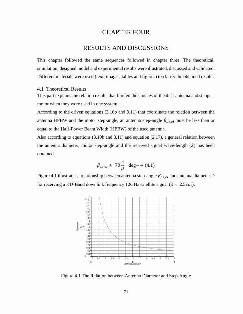
71

CHAPTER FOUR

4 RESULTS AND DISCUSSIONS

This chapter followed the same sequences followed in chapter three. The theoretical,

simulation, designed model and experimental results were illustrated, discussed and validated.

Different materials were used (text, images, tables and figures) to clarify the obtained results.

4.1 Theoretical Results

This part explains the relation results that limited the choices of the dish-antenna and stepper-

motor when they were used in one system.

According to the driven equations (3.10b and 3.11) that coordinate the relation between the

antenna HPBW and the motor step-angle, an antenna step-angle 𝛽𝑎𝑧,𝑒𝑙 must be less than or

equal to the Half-Power Beam Width (HPBW) of the used antenna.

Also according to equations (3.10b and 3.11) and equation (2.17), a general relation between

the antenna diameter, motor step-angle and the received signal wave-length (𝜆) has been

obtained.

𝛽𝑎𝑧,𝑒𝑙 ≤ 70𝜆

𝐷 deg−→ (4.1)

Figure 4.1 illustrates a relationship between antenna step-angle 𝛽𝑎𝑧,𝑒𝑙 and antenna diameter D

for receiving a KU-Band downlink frequency 12GHz satellite signal (𝜆 ≈ 2.5𝑐𝑚).

Figure 4.1 The Relation between Antenna Diameter and Step-Angle

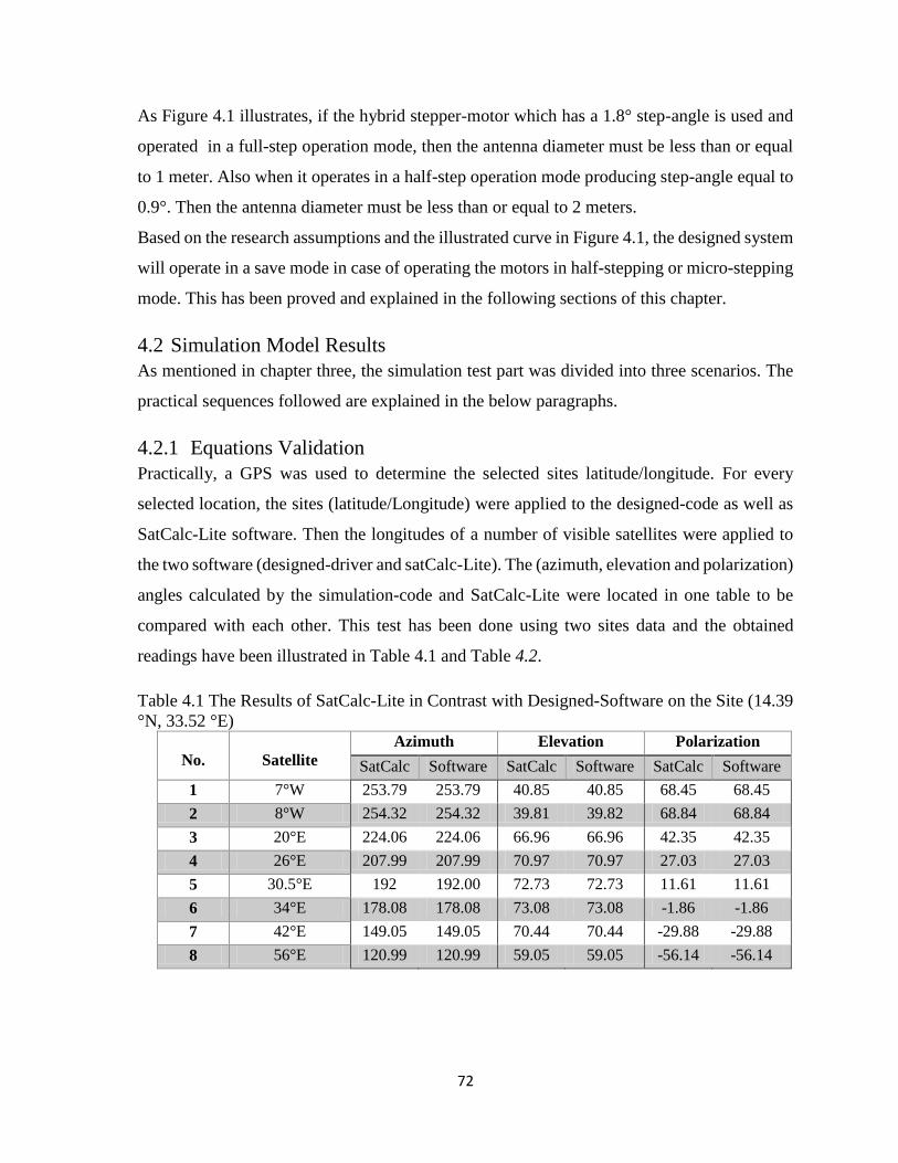
72

As Figure 4.1 illustrates, if the hybrid stepper-motor which has a 1.8° step-angle is used and

operated in a full-step operation mode, then the antenna diameter must be less than or equal

to 1 meter. Also when it operates in a half-step operation mode producing step-angle equal to

0.9°. Then the antenna diameter must be less than or equal to 2 meters.

Based on the research assumptions and the illustrated curve in Figure 4.1, the designed system

will operate in a save mode in case of operating the motors in half-stepping or micro-stepping

mode. This has been proved and explained in the following sections of this chapter.

4.2 Simulation Model Results

As mentioned in chapter three, the simulation test part was divided into three scenarios. The

practical sequences followed are explained in the below paragraphs.

4.2.1 Equations Validation

Practically, a GPS was used to determine the selected sites latitude/longitude. For every

selected location, the sites (latitude/Longitude) were applied to the designed-code as well as

SatCalc-Lite software. Then the longitudes of a number of visible satellites were applied to

the two software (designed-driver and satCalc-Lite). The (azimuth, elevation and polarization)

angles calculated by the simulation-code and SatCalc-Lite were located in one table to be

compared with each other. This test has been done using two sites data and the obtained

readings have been illustrated in Table 4.1 and Table 4.2.

Table 4.1 The Results of SatCalc-Lite in Contrast with Designed-Software on the Site (14.39

°N, 33.52 °E)

No.

Satellite

Azimuth Elevation Polarization

SatCalc Software SatCalc Software SatCalc Software

1 7°W 253.79 253.79 40.85 40.85 68.45 68.45

2 8°W 254.32 254.32 39.81 39.82 68.84 68.84

3 20°E 224.06 224.06 66.96 66.96 42.35 42.35

4 26°E 207.99 207.99 70.97 70.97 27.03 27.03

5 30.5°E 192 192.00 72.73 72.73 11.61 11.61

6 34°E 178.08 178.08 73.08 73.08 -1.86 -1.86

7 42°E 149.05 149.05 70.44 70.44 -29.88 -29.88

8 56°E 120.99 120.99 59.05 59.05 -56.14 -56.14

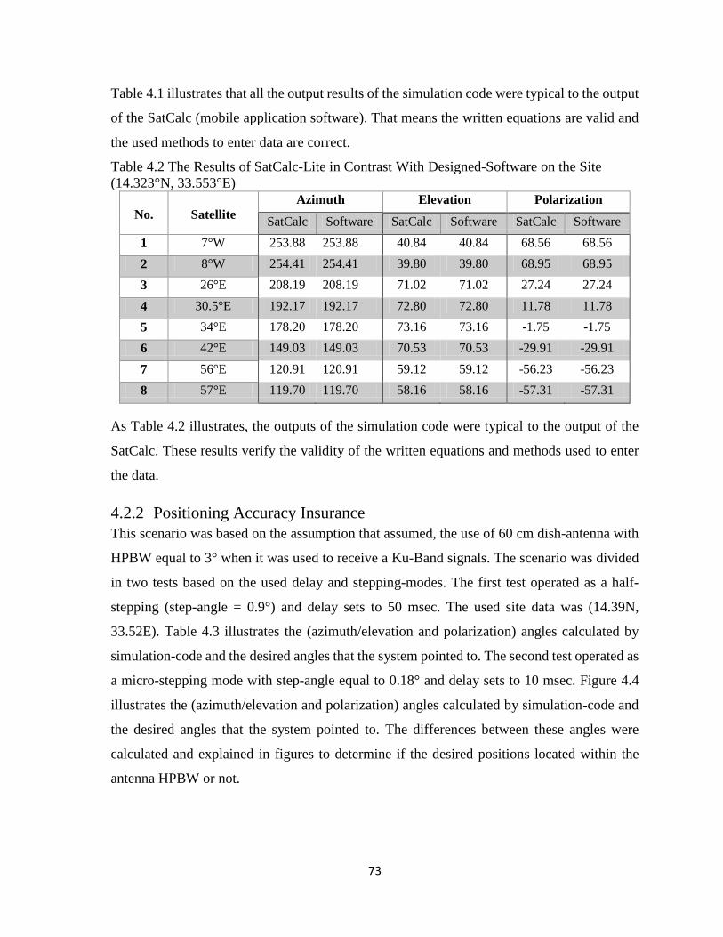
73

Table 4.1 illustrates that all the output results of the simulation code were typical to the output

of the SatCalc (mobile application software). That means the written equations are valid and

the used methods to enter data are correct.

Table 4.2 The Results of SatCalc-Lite in Contrast With Designed-Software on the Site

(14.323°N, 33.553°E)

No.

Satellite


SatCalc Software SatCalc Software SatCalc Software

1 7°W 253.88 253.88 40.84 40.84 68.56 68.56

2 8°W 254.41 254.41 39.80 39.80 68.95 68.95

3 26°E 208.19 208.19 71.02 71.02 27.24 27.24

4 30.5°E 192.17 192.17 72.80 72.80 11.78 11.78

5 34°E 178.20 178.20 73.16 73.16 -1.75 -1.75

6 42°E 149.03 149.03 70.53 70.53 -29.91 -29.91

7 56°E 120.91 120.91 59.12 59.12 -56.23 -56.23

8 57°E 119.70 119.70 58.16 58.16 -57.31 -57.31

As Table 4.2 illustrates, the outputs of the simulation code were typical to the output of the

SatCalc. These results verify the validity of the written equations and methods used to enter

the data.

4.2.2 Positioning Accuracy Insurance

This scenario was based on the assumption that assumed, the use of 60 cm dish-antenna with

HPBW equal to 3° when it was used to receive a Ku-Band signals. The scenario was divided

in two tests based on the used delay and stepping-modes. The first test operated as a half-

stepping (step-angle = 0.9°) and delay sets to 50 msec. The used site data was (14.39N,

33.52E). Table 4.3 illustrates the (azimuth/elevation and polarization) angles calculated by

simulation-code and the desired angles that the system pointed to. The second test operated as

a micro-stepping mode with step-angle equal to 0.18° and delay sets to 10 msec. Figure 4.4

illustrates the (azimuth/elevation and polarization) angles calculated by simulation-code and

the desired angles that the system pointed to. The differences between these angles were

calculated and explained in figures to determine if the desired positions located within the

antenna HPBW or not.

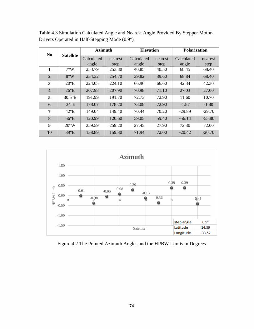
74

Table 4.3 Simulation Calculated Angle and Nearest Angle Provided By Stepper Motor-

Drivers Operated in Half-Stepping Mode (0.9°)

No

Satellite


Calculated

angle

nearest

step

Calculated

angle

nearest

step

Calculated

angle

nearest

step

1 7°W 253.79 253.80 40.85 40.50 68.45 68.40

2 8°W 254.32 254.70 39.82 39.60 68.84 68.40

3 20°E 224.05 224.10 66.96 66.60 42.34 42.30

4 26°E 207.98 207.90 70.98 71.10 27.03 27.00

5 30.5°E 191.99 191.70 72.73 72.90 11.60 10.70

6 34°E 178.07 178.20 73.08 72.90 -1.87 -1.80

7 42°E 149.04 149.40 70.44 70.20 -29.89 -29.70

8 56°E 120.99 120.60 59.05 59.40 -56.14 -55.80

9 20°W 259.59 259.20 27.45 27.90 72.30 72.00

10 39°E 158.89 159.30 71.94 72.00 -20.42 -20.70

Figure 4.2 The Pointed Azimuth Angles and the HPBW Limits in Degrees

-0.01

-0.38

-0.050.08

0.29

-0.13

-0.36

0.39 0.39

-0.41

-1.50

-1.00

-0.50

0.00

0.50

1.00

1.50

0 2 4 6 8 10

HP

BW

Lim

it

Satellite

Azimuth

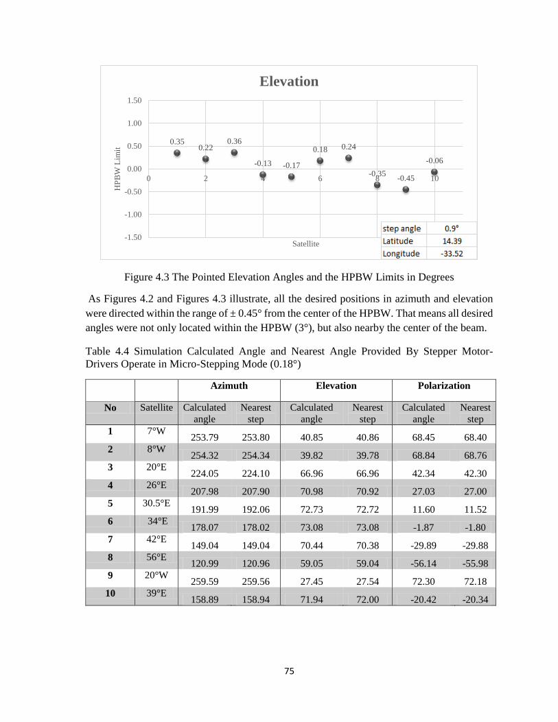
75

Figure 4.3 The Pointed Elevation Angles and the HPBW Limits in Degrees

As Figures 4.2 and Figures 4.3 illustrate, all the desired positions in azimuth and elevation

were directed within the range of ± 0.45° from the center of the HPBW. That means all desired

angles were not only located within the HPBW (3°), but also nearby the center of the beam.

Table 4.4 Simulation Calculated Angle and Nearest Angle Provided By Stepper Motor-

Drivers Operate in Micro-Stepping Mode (0.18°)


No Satellite Calculated

angle

Nearest

step

Calculated

angle

Nearest

step

Calculated

angle

Nearest

step

1 7°W 253.79 253.80 40.85 40.86 68.45 68.40

2 8°W 254.32 254.34 39.82 39.78 68.84 68.76

3 20°E 224.05 224.10 66.96 66.96 42.34 42.30

4 26°E 207.98 207.90 70.98 70.92 27.03 27.00

5 30.5°E 191.99 192.06 72.73 72.72 11.60 11.52

6 34°E 178.07 178.02 73.08 73.08 -1.87 -1.80

7 42°E 149.04 149.04 70.44 70.38 -29.89 -29.88

8 56°E 120.99 120.96 59.05 59.04 -56.14 -55.98

9 20°W 259.59 259.56 27.45 27.54 72.30 72.18

10 39°E 158.89 158.94 71.94 72.00 -20.42 -20.34

0.350.22

0.36

-0.13 -0.17

0.18 0.24

-0.35-0.45

-0.06

-1.50

-1.00

-0.50

0.00

0.50

1.00

1.50

0 2 4 6 8 10

HP

BW

Lim

it

Satellite

Elevation

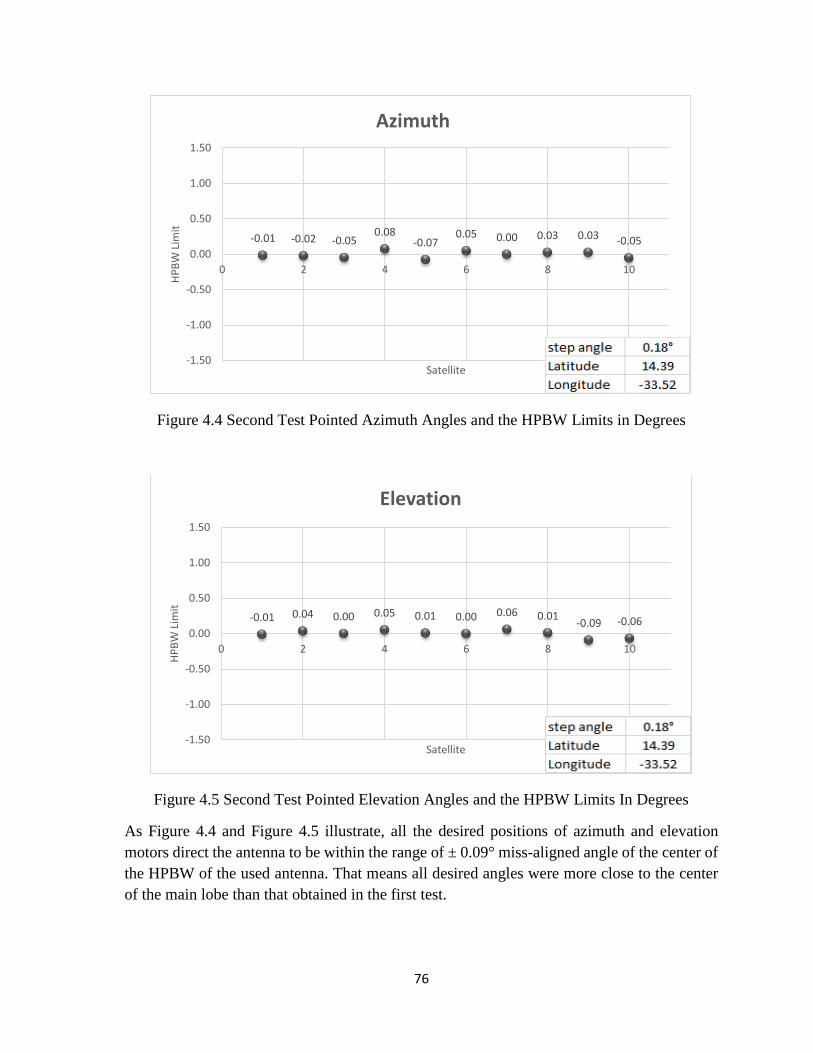
76

Figure 4.4 Second Test Pointed Azimuth Angles and the HPBW Limits in Degrees

Figure 4.5 Second Test Pointed Elevation Angles and the HPBW Limits In Degrees

As Figure 4.4 and Figure 4.5 illustrate, all the desired positions of azimuth and elevation

motors direct the antenna to be within the range of ± 0.09° miss-aligned angle of the center of

the HPBW of the used antenna. That means all desired angles were more close to the center

of the main lobe than that obtained in the first test.

-0.01 -0.02 -0.050.08

-0.070.05 0.00 0.03 0.03 -0.05

-1.50

-1.00

-0.50

0.00

0.50

1.00

1.50

0 2 4 6 8 10

HP

BW

Lim

it

Satellite

Azimuth

-0.01 0.04 0.00 0.05 0.01 0.00 0.06 0.01-0.09 -0.06

-1.50

-1.00

-0.50

0.00

0.50

1.00

1.50

0 2 4 6 8 10

HP

BW

Lim

it

Satellite

Elevation

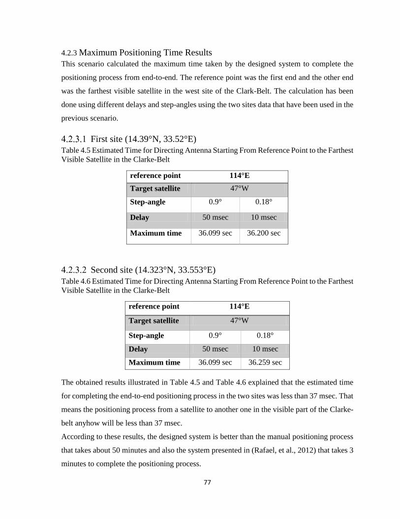
77

4.2.3 Maximum Positioning Time Results

This scenario calculated the maximum time taken by the designed system to complete the

positioning process from end-to-end. The reference point was the first end and the other end

was the farthest visible satellite in the west site of the Clark-Belt. The calculation has been

done using different delays and step-angles using the two sites data that have been used in the

previous scenario.

First site (14.39°N, 33.52°E)

Table 4.5 Estimated Time for Directing Antenna Starting From Reference Point to the Farthest

Visible Satellite in the Clarke-Belt

reference point 114°E

Target satellite 47°W

Step-angle 0.9° 0.18°

Delay 50 msec 10 msec

Maximum time 36.099 sec 36.200 sec

Second site (14.323°N, 33.553°E)

Table 4.6 Estimated Time for Directing Antenna Starting From Reference Point to the Farthest

Visible Satellite in the Clarke-Belt

reference point 114°E

Target satellite 47°W

Step-angle 0.9° 0.18°

Delay 50 msec 10 msec

Maximum time 36.099 sec 36.259 sec

The obtained results illustrated in Table 4.5 and Table 4.6 explained that the estimated time

for completing the end-to-end positioning process in the two sites was less than 37 msec. That

means the positioning process from a satellite to another one in the visible part of the Clarke-

belt anyhow will be less than 37 msec.

According to these results, the designed system is better than the manual positioning process

that takes about 50 minutes and also the system presented in (Rafael, et al., 2012) that takes 3

minutes to complete the positioning process.

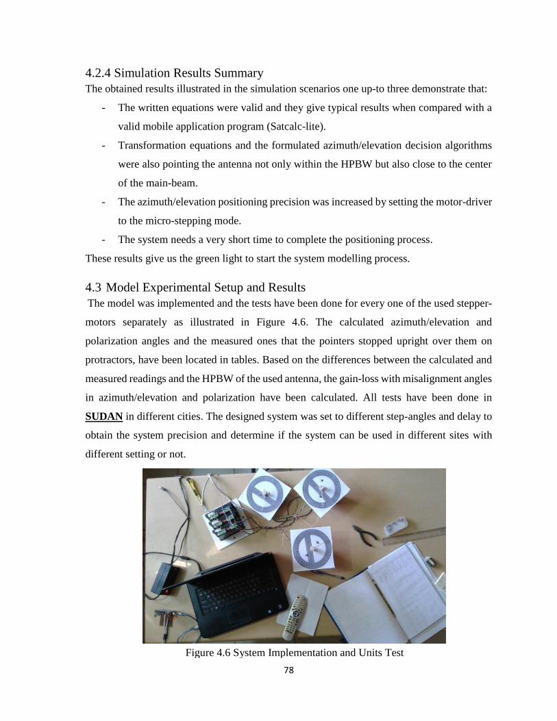
78

Figure 4.6 System Implementation and Units Test

4.2.4 Simulation Results Summary

The obtained results illustrated in the simulation scenarios one up-to three demonstrate that:

- The written equations were valid and they give typical results when compared with a

valid mobile application program (Satcalc-lite).

- Transformation equations and the formulated azimuth/elevation decision algorithms

were also pointing the antenna not only within the HPBW but also close to the center

of the main-beam.

- The azimuth/elevation positioning precision was increased by setting the motor-driver

to the micro-stepping mode.

- The system needs a very short time to complete the positioning process.

These results give us the green light to start the system modelling process.

4.3 Model Experimental Setup and Results

The model was implemented and the tests have been done for every one of the used stepper-

motors separately as illustrated in Figure 4.6. The calculated azimuth/elevation and

polarization angles and the measured ones that the pointers stopped upright over them on

protractors, have been located in tables. Based on the differences between the calculated and

measured readings and the HPBW of the used antenna, the gain-loss with misalignment angles

in azimuth/elevation and polarization have been calculated. All tests have been done in

SUDAN in different cities. The designed system was set to different step-angles and delay to

obtain the system precision and determine if the system can be used in different sites with

different setting or not.

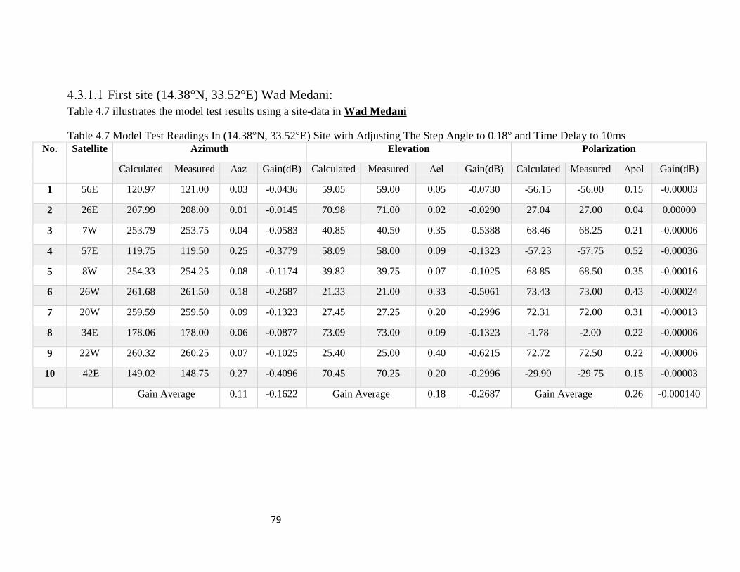
79

First site (14.38°N, 33.52°E) Wad Medani:

Table 4.7 illustrates the model test results using a site-data in Wad Medani

Table 4.7 Model Test Readings In (14.38°N, 33.52°E) Site with Adjusting The Step Angle to 0.18° and Time Delay to 10ms No. Satellite Azimuth Elevation Polarization

Calculated Measured Δaz Gain(dB) Calculated Measured Δel Gain(dB) Calculated Measured Δpol Gain(dB)

1 56E 120.97 121.00 0.03 -0.0436 59.05 59.00 0.05 -0.0730 -56.15 -56.00 0.15 -0.00003

2 26E 207.99 208.00 0.01 -0.0145 70.98 71.00 0.02 -0.0290 27.04 27.00 0.04 0.00000

3 7W 253.79 253.75 0.04 -0.0583 40.85 40.50 0.35 -0.5388 68.46 68.25 0.21 -0.00006

4 57E 119.75 119.50 0.25 -0.3779 58.09 58.00 0.09 -0.1323 -57.23 -57.75 0.52 -0.00036

5 8W 254.33 254.25 0.08 -0.1174 39.82 39.75 0.07 -0.1025 68.85 68.50 0.35 -0.00016

6 26W 261.68 261.50 0.18 -0.2687 21.33 21.00 0.33 -0.5061 73.43 73.00 0.43 -0.00024

7 20W 259.59 259.50 0.09 -0.1323 27.45 27.25 0.20 -0.2996 72.31 72.00 0.31 -0.00013

8 34E 178.06 178.00 0.06 -0.0877 73.09 73.00 0.09 -0.1323 -1.78 -2.00 0.22 -0.00006

9 22W 260.32 260.25 0.07 -0.1025 25.40 25.00 0.40 -0.6215 72.72 72.50 0.22 -0.00006

10 42E 149.02 148.75 0.27 -0.4096 70.45 70.25 0.20 -0.2996 -29.90 -29.75 0.15 -0.00003

Gain Average 0.11 -0.1622 Gain Average 0.18 -0.2687 Gain Average 0.26 -0.000140

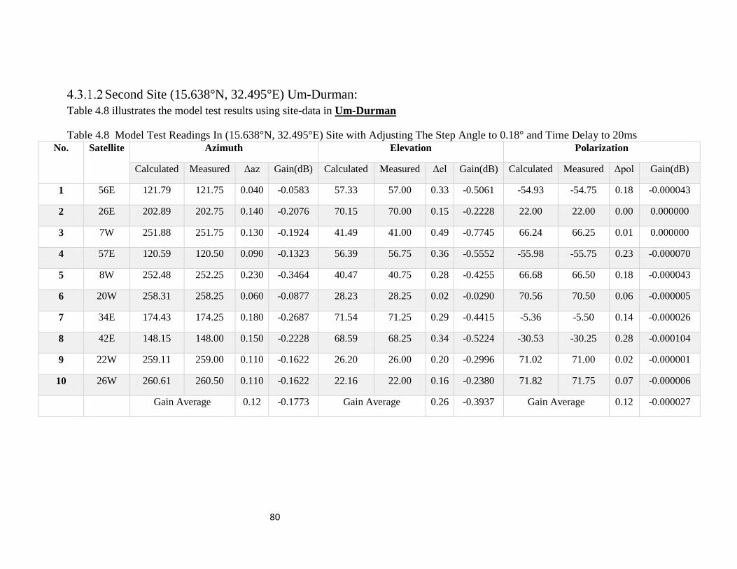
80

Second Site (15.638°N, 32.495°E) Um-Durman:

Table 4.8 illustrates the model test results using site-data in Um-Durman


Calculated Measured Δaz Gain(dB) Calculated Measured Δel Gain(dB) Calculated Measured Δpol Gain(dB)

1 56E 121.79 121.75 0.040 -0.0583 57.33 57.00 0.33 -0.5061 -54.93 -54.75 0.18 -0.000043

2 26E 202.89 202.75 0.140 -0.2076 70.15 70.00 0.15 -0.2228 22.00 22.00 0.00 0.000000

3 7W 251.88 251.75 0.130 -0.1924 41.49 41.00 0.49 -0.7745 66.24 66.25 0.01 0.000000

4 57E 120.59 120.50 0.090 -0.1323 56.39 56.75 0.36 -0.5552 -55.98 -55.75 0.23 -0.000070

5 8W 252.48 252.25 0.230 -0.3464 40.47 40.75 0.28 -0.4255 66.68 66.50 0.18 -0.000043

6 20W 258.31 258.25 0.060 -0.0877 28.23 28.25 0.02 -0.0290 70.56 70.50 0.06 -0.000005

7 34E 174.43 174.25 0.180 -0.2687 71.54 71.25 0.29 -0.4415 -5.36 -5.50 0.14 -0.000026

8 42E 148.15 148.00 0.150 -0.2228 68.59 68.25 0.34 -0.5224 -30.53 -30.25 0.28 -0.000104

9 22W 259.11 259.00 0.110 -0.1622 26.20 26.00 0.20 -0.2996 71.02 71.00 0.02 -0.000001

10 26W 260.61 260.50 0.110 -0.1622 22.16 22.00 0.16 -0.2380 71.82 71.75 0.07 -0.000006


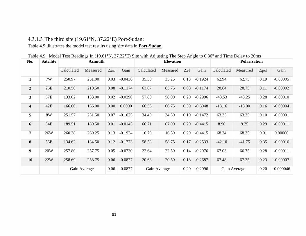
81

The third site (19.61°N, 37.22°E) Port-Sudan:

Table 4.9 illustrates the model test results using site data in Port-Sudan


Calculated Measured Δaz Gain Calculated Measured Δel Gain Calculated Measured Δpol Gain

1 7W 250.97 251.00 0.03 -0.0436 35.38 35.25 0.13 -0.1924 62.94 62.75 0.19 -0.00005

2 26E 210.58 210.50 0.08 -0.1174 63.67 63.75 0.08 -0.1174 28.64 28.75 0.11 -0.00002

3 57E 133.02 133.00 0.02 -0.0290 57.80 58.00 0.20 -0.2996 -43.53 -43.25 0.28 -0.00010

4 42E 166.00 166.00 0.00 0.0000 66.36 66.75 0.39 -0.6048 -13.16 -13.00 0.16 -0.00004

5 8W 251.57 251.50 0.07 -0.1025 34.40 34.50 0.10 -0.1472 63.35 63.25 0.10 -0.00001

6 34E 189.51 189.50 0.01 -0.0145 66.71 67.00 0.29 -0.4415 8.96 9.25 0.29 -0.00011

7 26W 260.38 260.25 0.13 -0.1924 16.79 16.50 0.29 -0.4415 68.24 68.25 0.01 0.00000

8 56E 134.62 134.50 0.12 -0.1773 58.58 58.75 0.17 -0.2533 -42.10 -41.75 0.35 -0.00016

9 20W 257.80 257.75 0.05 -0.0730 22.64 22.50 0.14 -0.2076 67.03 66.75 0.28 -0.00011

10 22W 258.69 258.75 0.06 -0.0877 20.68 20.50 0.18 -0.2687 67.48 67.25 0.23 -0.00007


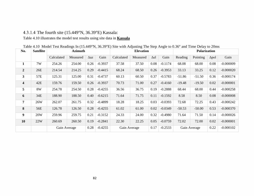
82

The fourth site (15.449°N, 36.39°E) Kassala:

Table 4.10 illustrates the model test results using site data in Kassala


Calculated Measured Δaz Gain Calculated Measured Δel Gain Reading Pointing Δpol Gain

1 7W 254.26 254.00 0.26 -0.3937 37.58 37.50 0.08 -0.1174 68.08 68.00 0.08 -0.000009

2 26E 214.54 214.25 0.29 -0.4415 68.24 68.50 0.26 -0.3953 33.13 33.25 0.12 -0.000020

3 57E 125.31 125.00 0.31 -0.4737 60.13 60.50 0.37 -0.5783 -51.86 -51.50 0.36 -0.000174

4 42E 159.76 159.50 0.26 -0.3937 70.73 71.00 0.27 -0.4160 -19.48 -19.50 0.02 -0.000001

5 8W 254.78 254.50 0.28 -0.4255 36.56 36.75 0.19 -0.2888 68.44 68.00 0.44 -0.000258

6 34E 188.90 188.50 0.40 -0.6215 71.64 71.75 0.11 -0.1592 8.58 8.50 0.08 -0.000008

7 26W 262.07 261.75 0.32 -0.4899 18.28 18.25 0.03 -0.0393 72.68 72.25 0.43 -0.000242

8 56E 126.78 126.50 0.28 -0.4255 61.02 61.00 0.02 -0.0349 -50.53 -50.00 0.53 -0.000370

9 20W 259.96 259.75 0.21 -0.3152 24.33 24.00 0.32 -0.4980 71.64 71.50 0.14 -0.000026

10 22W 260.69 260.50 0.19 -0.2841 22.30 22.25 0.05 -0.0759 72.02 72.00 0.02 -0.000001


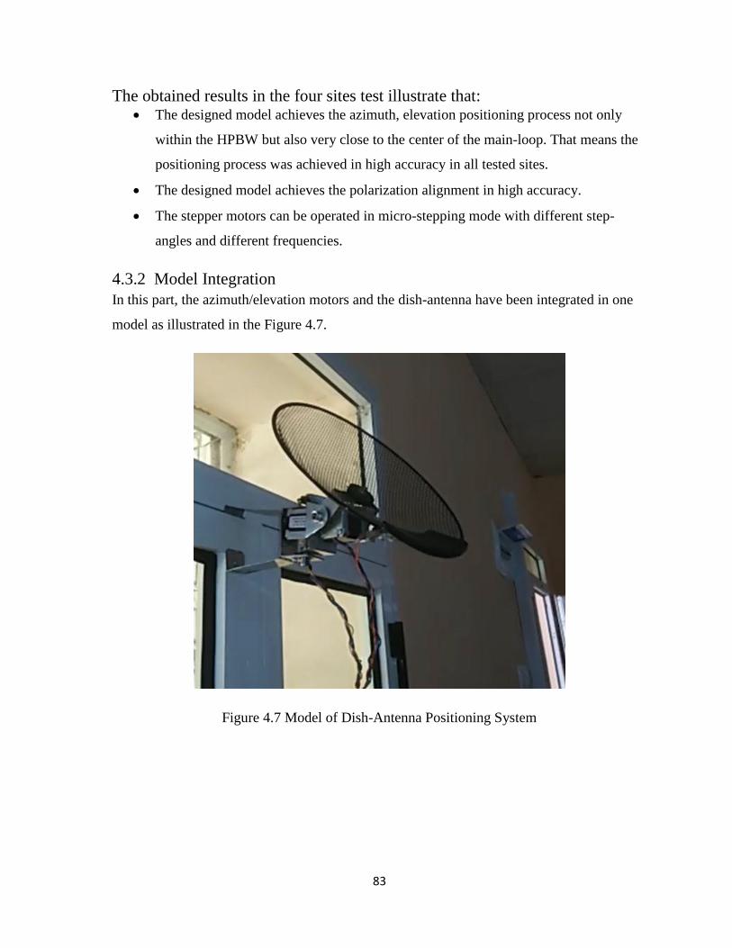
83

The obtained results in the four sites test illustrate that: The designed model achieves the azimuth, elevation positioning process not only

within the HPBW but also very close to the center of the main-loop. That means the

positioning process was achieved in high accuracy in all tested sites.

The designed model achieves the polarization alignment in high accuracy.

The stepper motors can be operated in micro-stepping mode with different step-

angles and different frequencies.

4.3.2 Model Integration

In this part, the azimuth/elevation motors and the dish-antenna have been integrated in one

model as illustrated in the Figure 4.7.

Figure 4.7 Model of Dish-Antenna Positioning System

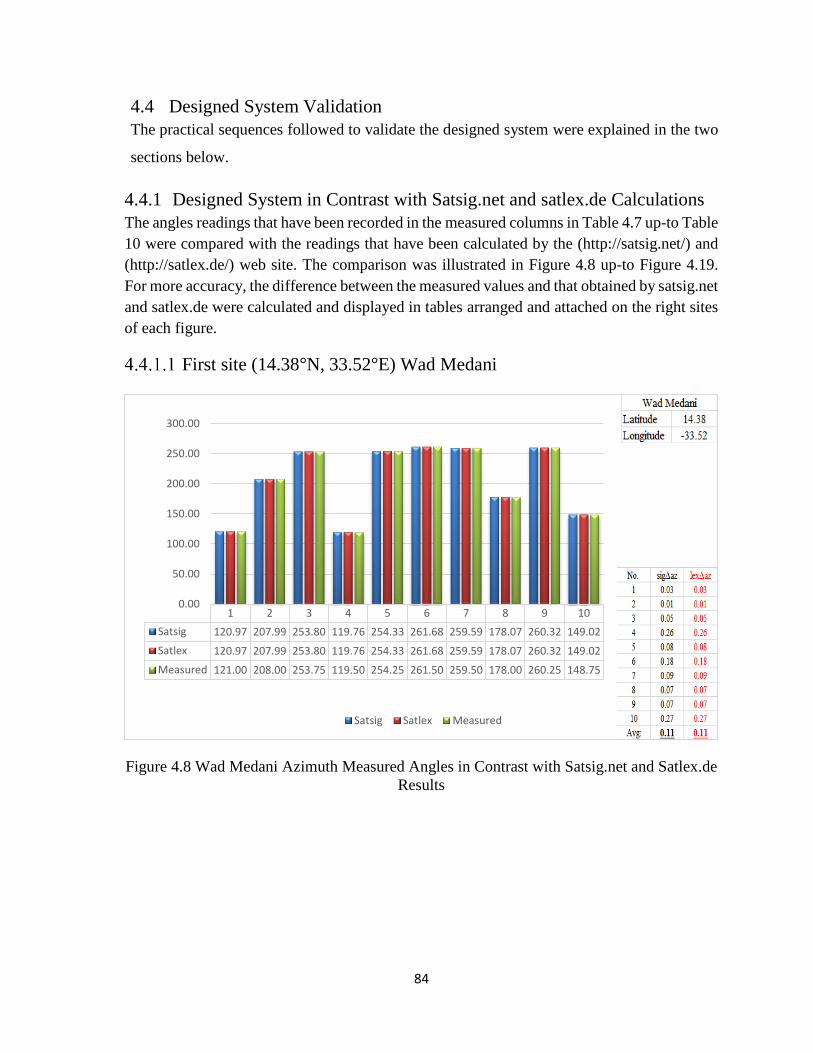
84

4.4 Designed System Validation

The practical sequences followed to validate the designed system were explained in the two

sections below.

4.4.1 Designed System in Contrast with Satsig.net and satlex.de Calculations

The angles readings that have been recorded in the measured columns in Table 4.7 up-to Table

10 were compared with the readings that have been calculated by the (http://satsig.net/) and

(http://satlex.de/) web site. The comparison was illustrated in Figure 4.8 up-to Figure 4.19.

For more accuracy, the difference between the measured values and that obtained by satsig.net

and satlex.de were calculated and displayed in tables arranged and attached on the right sites

of each figure.

First site (14.38°N, 33.52°E) Wad Medani

Figure 4.8 Wad Medani Azimuth Measured Angles in Contrast with Satsig.net and Satlex.de

Results

1 2 3 4 5 6 7 8 9 10

Satsig 120.97 207.99 253.80 119.76 254.33 261.68 259.59 178.07 260.32 149.02

Satlex 120.97 207.99 253.80 119.76 254.33 261.68 259.59 178.07 260.32 149.02

Measured 121.00 208.00 253.75 119.50 254.25 261.50 259.50 178.00 260.25 148.75

0.00

50.00

100.00

150.00

200.00

250.00

300.00

Satsig Satlex Measured

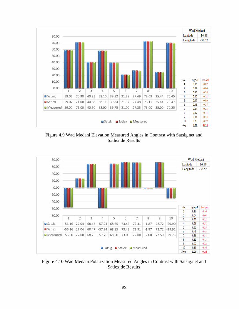
85

Figure 4.9 Wad Medani Elevation Measured Angles in Contrast with Satsig.net and

Satlex.de Results

Figure 4.10 Wad Medani Polarization Measured Angles in Contrast with Satsig.net and

Satlex.de Results

1 2 3 4 5 6 7 8 9 10

Satsig 59.06 70.98 40.85 58.10 39.82 21.38 27.49 73.09 25.44 70.45

Satlex 59.07 71.00 40.88 58.11 39.84 21.37 27.48 73.11 25.44 70.47

Measured 59.00 71.00 40.50 58.00 39.75 21.00 27.25 73.00 25.00 70.25

0.00

10.00

20.00

30.00

40.00

50.00

60.00

70.00

80.00


1 2 3 4 5 6 7 8 9 10

Satsig -56.16 27.04 68.47 -57.24 68.85 73.43 72.31 -1.87 72.72 -29.90

Satlex -56.16 27.04 68.47 -57.24 68.85 73.43 72.31 -1.87 72.72 -29.91

Measured -56.00 27.00 68.25 -57.75 68.50 73.00 72.00 -2.00 72.50 -29.75

-80.00

-60.00

-40.00

-20.00

0.00

20.00

40.00

60.00

80.00


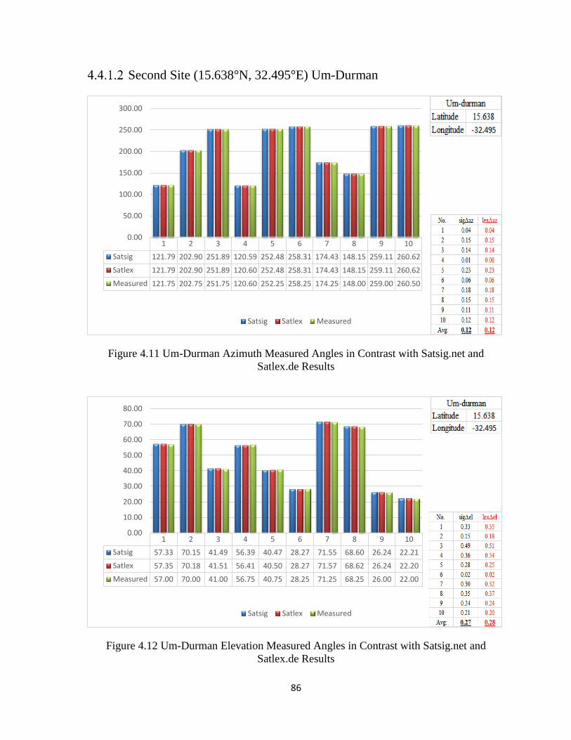
86

Second Site (15.638°N, 32.495°E) Um-Durman

Figure 4.11 Um-Durman Azimuth Measured Angles in Contrast with Satsig.net and

Satlex.de Results

Figure 4.12 Um-Durman Elevation Measured Angles in Contrast with Satsig.net and

Satlex.de Results

1 2 3 4 5 6 7 8 9 10

Satsig 121.79 202.90 251.89 120.59 252.48 258.31 174.43 148.15 259.11 260.62

Satlex 121.79 202.90 251.89 120.60 252.48 258.31 174.43 148.15 259.11 260.62

Measured 121.75 202.75 251.75 120.60 252.25 258.25 174.25 148.00 259.00 260.50

0.00

50.00

100.00

150.00

200.00

250.00

300.00


1 2 3 4 5 6 7 8 9 10

Satsig 57.33 70.15 41.49 56.39 40.47 28.27 71.55 68.60 26.24 22.21

Satlex 57.35 70.18 41.51 56.41 40.50 28.27 71.57 68.62 26.24 22.20

Measured 57.00 70.00 41.00 56.75 40.75 28.25 71.25 68.25 26.00 22.00

0.00

10.00

20.00

30.00

40.00

50.00

60.00

70.00

80.00


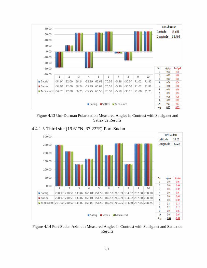
87

Figure 4.13 Um-Durman Polarization Measured Angles in Contrast with Satsig.net and

Satlex.de Results

Third site (19.61°N, 37.22°E) Port-Sudan

Figure 4.14 Port-Sudan Azimuth Measured Angles in Contrast with Satsig.net and Satlex.de

Results

1 2 3 4 5 6 7 8 9 10

Satsig -54.94 22.00 66.24 -55.99 66.68 70.56 -5.36 -30.54 71.02 71.82

Satlex -54.94 22.00 66.24 -55.99 66.68 70.56 -5.36 -30.54 71.02 71.82

Measured -54.75 22.00 66.25 -55.75 66.50 70.50 -5.50 -30.25 71.00 71.75

-80.00

-60.00

-40.00

-20.00

0.00

20.00

40.00

60.00

80.00


1 2 3 4 5 6 7 8 9 10

Satsig 250.97 210.59 133.02 166.01 251.58 189.52 260.39 134.62 257.80 258.70

Satlex 250.97 210.59 133.02 166.01 251.58 189.52 260.39 134.62 257.80 258.70

Measured 251.00 210.50 133.00 166.00 251.50 189.50 260.25 134.50 257.75 258.75

0.00

50.00

100.00

150.00

200.00

250.00

300.00


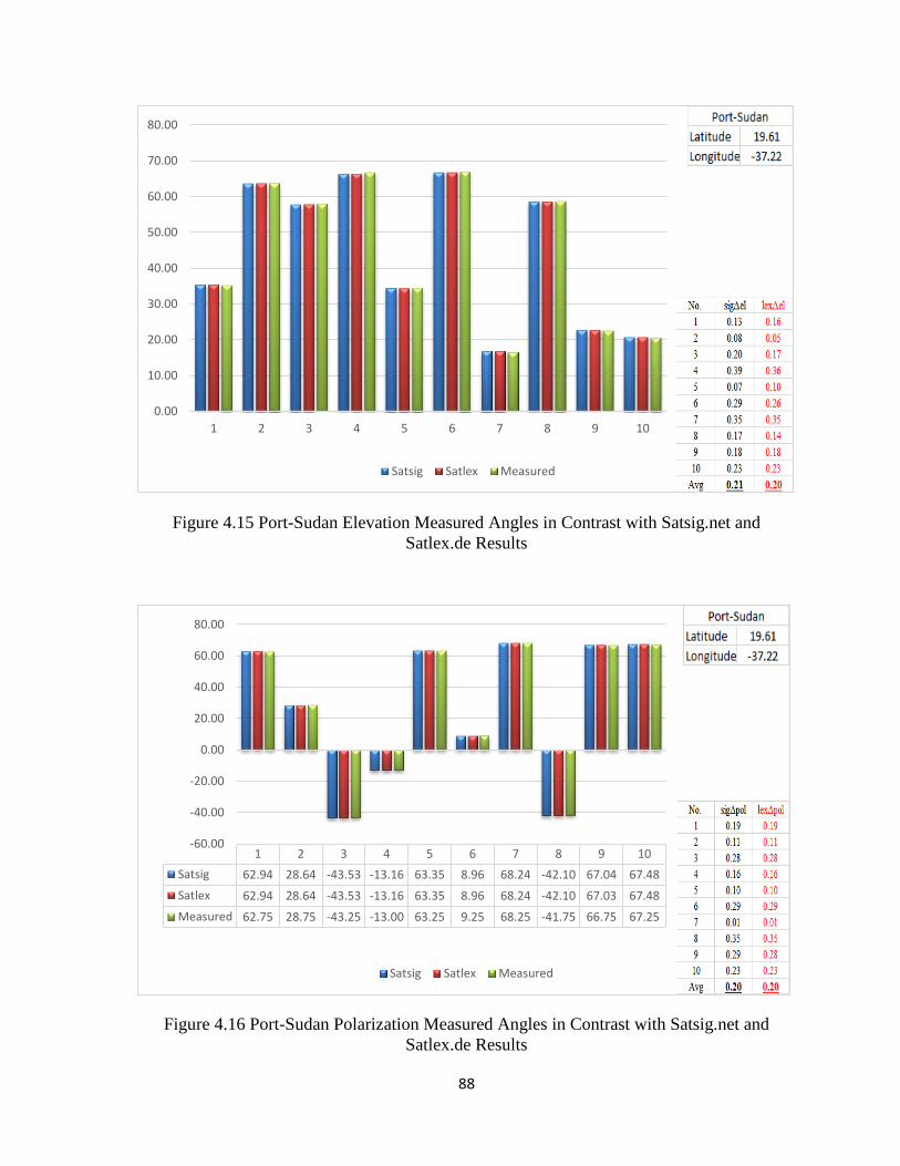
88

Figure 4.15 Port-Sudan Elevation Measured Angles in Contrast with Satsig.net and

Satlex.de Results

Figure 4.16 Port-Sudan Polarization Measured Angles in Contrast with Satsig.net and

Satlex.de Results

0.00

10.00

20.00

30.00

40.00

50.00

60.00

70.00

80.00

1 2 3 4 5 6 7 8 9 10


1 2 3 4 5 6 7 8 9 10

Satsig 62.94 28.64 -43.53 -13.16 63.35 8.96 68.24 -42.10 67.04 67.48

Satlex 62.94 28.64 -43.53 -13.16 63.35 8.96 68.24 -42.10 67.03 67.48

Measured 62.75 28.75 -43.25 -13.00 63.25 9.25 68.25 -41.75 66.75 67.25

-60.00

-40.00

-20.00

0.00

20.00

40.00

60.00

80.00


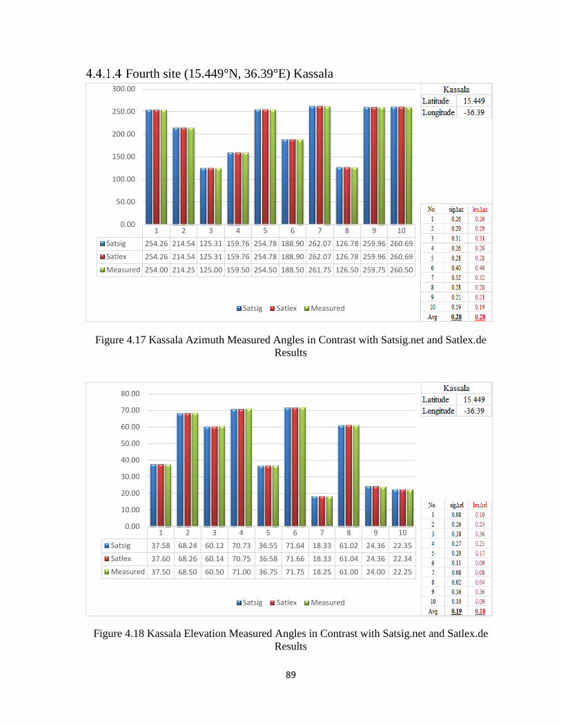
89

Fourth site (15.449°N, 36.39°E) Kassala

Figure 4.17 Kassala Azimuth Measured Angles in Contrast with Satsig.net and Satlex.de

Results

Figure 4.18 Kassala Elevation Measured Angles in Contrast with Satsig.net and Satlex.de

Results

1 2 3 4 5 6 7 8 9 10

Satsig 254.26 214.54 125.31 159.76 254.78 188.90 262.07 126.78 259.96 260.69

Satlex 254.26 214.54 125.31 159.76 254.78 188.90 262.07 126.78 259.96 260.69

Measured 254.00 214.25 125.00 159.50 254.50 188.50 261.75 126.50 259.75 260.50

0.00

50.00

100.00

150.00

200.00

250.00

300.00


1 2 3 4 5 6 7 8 9 10

Satsig 37.58 68.24 60.12 70.73 36.55 71.64 18.33 61.02 24.36 22.35

Satlex 37.60 68.26 60.14 70.75 36.58 71.66 18.33 61.04 24.36 22.34

Measured 37.50 68.50 60.50 71.00 36.75 71.75 18.25 61.00 24.00 22.25

0.00

10.00

20.00

30.00

40.00

50.00

60.00

70.00

80.00


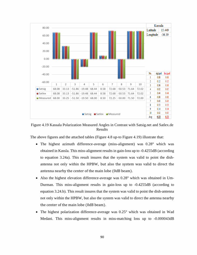
90

Figure 4.19 Kassala Polarization Measured Angles in Contrast with Satsig.net and Satlex.de

Results

The above figures and the attached tables (Figure 4.8 up-to Figure 4.19) illustrate that:

The highest azimuth difference-average (miss-alignment) was 0.28° which was

obtained in Kassla. This miss-alignment results in gain-loss up to -0.4255dB (according

to equation 3.24a). This result insures that the system was valid to point the dish-

antenna not only within the HPBW, but also the system was valid to direct the

antenna nearby the center of the main lobe (0dB beam).

Also the highest elevation difference-average was 0.28° which was obtained in Um-

Durman. This miss-alignment results in gain-loss up to -0.4255dB (according to

equation 3.24.b). This result insures that the system was valid to point the dish-antenna

not only within the HPBW, but also the system was valid to direct the antenna nearby

the center of the main lobe (0dB beam).

The highest polarization difference-average was 0.25° which was obtained in Wad

Medani. This miss-alignment results in miss-matching loss up to -0.000043dB

1 2 3 4 5 6 7 8 9 10

Satsig 68.08 33.13 -51.86 -19.48 68.44 8.58 72.68 -50.53 71.64 72.02

Satlex 68.08 33.13 -51.86 -19.48 68.44 8.58 72.68 -50.53 71.64 72.02

Measured 68.00 33.25 -51.50 -19.50 68.00 8.50 72.25 -50.00 71.50 72.00

-60.00

-40.00

-20.00

0.00

20.00

40.00

60.00

80.00


91

(according to equation 3.24.c). This result insures that the system was valid to align the

LNB with the satellite signal source.

4.4.2 Comparison between the Designed System and Related Studies

The properties of the designed system were highlighted and compared with that mentioned

in the related studies. The comparison was done based on a number of points shown in the

below points.

Positioning Time

The designed system achieved the positioning task with high accuracy in not more than

40 seconds instead of a number of minutes taken by the other systems or consuming long

time in manual positioning process.

Polarization alignment

The designed system is concerned with adjusting the antenna polarization as well as

pointing the antenna in azimuth and elevation.

Reduce the hardware and avoid complexity

The research focused in designing and developing the software-driver to reduce the

hardware that was found in the closed-loop systems and avoid the complexity of the PID,

PI and LQR controllers. Also to reduce the hardware, the designed system was based on

micro-controller and IR-remote control instead of PC.

Simple to use and develop

The designed system uses new technology (Arduino micro-controller) that was very

simple to be implemented and developed. Also it is simple to be handled by the user

because it uses a familiar tool to be controlled (public IR-remote control).

Portable System

The designed system can be tested in different sites all-round the northern hemisphere. It

needs only updating the site-data (latitude, longitude).

92

CHAPTER FIVE

CONCLUSIONS AND RECOMMENDATIONS

5.1 Conclusions

Based on the theories, methodology, experimental results and discussions illustrated in the

previous chapters, the designed model which was based on microcontroller Arduino Uno card,

stepper-motors and IR-remote control, achieves the goal of the research (design a small dish-

antenna control system model for receiving signals from geostationary satellites operating in

Ku-band). The designed model was tested using different sites data (longitude, latitude) for

different locations in Sudan (Wad Medani, Um-Durman, Port-Sudan and Kassala). The results

illustrate that the model achieves the azimuth/elevation positioning process in high precision.

The highest azimuth difference-average (miss-alignment) was 0.28° obtained in Kassla with

gain-loss up to -0.4255dB. Also the highest elevation difference-average was 0.28° obtained

in Um-Durman with gain-loss up to -0.4255dB. For the polarization, the highest difference-

average was 0.25° obtained in Wad Medani with miss-matching loss up to -0.000043dB. Also

the model improves the directing time. It takes 40 seconds to achieve the intended position

when compared with the previous studies where the minimum directing time was 3 minutes.

The research contributes in the satellite positioning systems in a number of issues that can be

arranged in: reducing the system hardware, avoiding the complexity of the closed-loop control

system that was found in existing systems, providing an effective positioning system, offering

a controlled system that can be embedded in the commercial IRDs or STBs, delivering an

easy-to-use technology for the users, navigating between satellites and increasing the number

of channels that can be watched.

5.2 Recommendations

The system was studied in sites in the northern part of the earth. The research

recommends the study of the designed system in the southern hemisphere as well as

in the northern one.

The research deals with studying the system software design and the general features

of the model and not caring for the antenna weight and the optimum motors torque

93

calculations. More works must be done in this part to operate the designed system in

a save mode.

Also the research recommends to apply this system in real to be validated by receiving

real signals from a number of visible satellites.

94

6 References

Abdul Rehman, Chishti; Bukhari, Syed Fasih-Ur-Rehman; Khaliq, Hafiz Saad; Khan,

Mohammad Hunain; Bukhari, Syed Zulfiqar Haider, 2014. Radio Telescope Antenna

Azimuth Position Control System Design and Analysis in Matlab/Simulink Using PID and

LQR Controller. Buletinul Institutului Politehnic Din Iaşi. LX (LXIV), Volume 3-4, pp. 45-

57.

Acarnley, P., (2007). Stepping Motors a Guide to Theory and Practice. 4th ed. United

Kingdom: The Institution of Enngineering and Technology.

Balanis, C. A., (2005). Antenna Theory Analysis and Design. 3rd ed. United States of

America: John Wiley and Sons.

Bhuyan, M. H., (2007). Wireless Control System for Dc Motor to Position a Dish Antenna

Using Microcomputer. Journal of Science and Technology, 2(1), pp. 44-49.

Brooks, D. R., (2015). Arduino-Based Dataloggers: Hardware and Software. Institute for

Earth Science Research and Education, Volume V 1.2.

Condit, R. and Jones, D. D. W., (2004). Stepping Motors Fundamentals. Microchip

Technology Inc., pp. 1-26.

Didactic, F., (2015). Satellite Orbits, Coverage, and Antenna Alignment. 1st ed. Canada: Festo

Didactic Ltee/Ltd.

Elbert, B. R., (2008). Introduction to Satellite Communication. 3rd ed. United States of

America: ARTECH HOUSE.

Evans, B. W., (2007). Arduino Programming Notebook. 1st ed. s.l.:Creative Commons

Attribution-Noncommercial-Share Alike 3.0 License..

Fung, C., (2011). Basic Antenna Theory and Application, s.l.: Project Number: SNM MQP

0414.

Grant, M., (2005). Quick Start for Beginners to Drive a Stepper Motor, Ver.1: Freescale

Semiconductor, Inc.

He, G., G.Li and Huang, M. L. a. Y., (2009). LQG Controller with Wind Gust Disturbance

Rejection Property for Cassegrain Antenna. s.l., Proceedings of IEEE International

Conference on Intelligent Computing and Intelligent Systems (ICIS),2: 344-348.

Jia, J and Qin, L. X. a. Y., (2009). Study of Adaptive Variable Structure Attitude Control and

its full Physical Simulation of Multi-Body Satellite Antenna Drive Control. , Proceedings of

World Congess on Computer and Information Engineering (WRI), 2: 546-549.

95

Kolawole, M. O., (2002). Satellite Communication Engineering. 1st ed. United States of

America,New York: Marcel Dekker.

Linus Aloo, A., Kihato, P. K. and Kamau, S. I., (2016). DC Servomotor-based Antenna

Positioning Control System Design using Hybrid PID-LQR Controller. European

International Journal of Science and Technology, 5(2), pp. 17-31.

Lwin, M. M. and Win, N. N., (2014). Microcontroller Based Smart Solar Tracking System.

International Journal of Scientific Engineering and Technology Research, 3(9), pp. 1845-

1859.

Me. Me, Tun, K. O. C. M. N. and Myo, H., (2012). Satellite Dish Positioning Control by DC

Motor Using IR Remote Control. International Journal of Electronics and Computer

Science Engineering, 3(3), pp. 199-207.

Milligan, T. A., (2005). MODERN ANTENNA DESIGN. 2nd ed. United States of America: A

JOHN WILEY and SONS.

Mohammed, A., Noor, S. B. B. M., Hassan, M. K. B. and Soh, A. B. C., (2014). A Review of

Strategies for Parabolic Antenna Control. Australian Journal of Basic and Applied Sciences,

8(7), pp. 135-148.

Mulla, A. A. and Vasambekar, P., (2017). Speed Rate Corrected Antenna Azimuth Axis

Positioning System. International Journal of Electronics Engineering Research, 9(2), pp.

151-158.

Nelson, D. R. A., (2014). Satellite Communication Design and Engineering. [Online]

Available at: http://www.aticourses.com/satellite_communications_systems.htm

[Accessed 28 July 2016].

Ogundele, A., D., E.C.A, A. H. and A, A. Y., (2010). Mathematical Modelling of Antenna

Look Angles of Geostationary Communications Satellite Using Two Models of Control

Stations. International Conference on Advanced Computer Theory and Engineering, 4(3),

pp. 236-240.

Okumus, H. İ., Sahin, E. and Akyazi, O., (2013). Antenna Azimuth Position Control with

Fuzzy Logic and Self-Tuning Fuzzy Logic Controllers. [Online]

Available at: http://www.emo.org.tr/ekler/30721392f46c410_ek.pdf

[Accessed 26 January (2017)].

Otieno, O. R., (2015). Solar Tracker For Solar Panel. University of Nairobi 2015, 24 April.

Prajwal, B., Grover, P. and Pannu, P., (2015). Remote Alignment of Dish Positioning By

Android Application. International Journal of Engineering Research and Management

Technology, 2(2), pp. 267-269.

96

Pran, S. K. et al., (1998). Microcomputer Based Dish Antenna Position Control System.

Dhaka, International Conference on Computer and Information Tech.

Purdum, P. J., (2012). Beginning C for Arduino. 1st ed. : Apress.

Rafael, M. C., Prado, J. B. G. and do, P. P. L., (2012). Development of an Automated System

for Maneuvering Parabolic Dish Antennas Used in Satellite Comunication. ABCM

Symposium Series in Mechatronics, 5(2), pp. 69-78.

Rajini, M. G. and Murthy, M. K. K., (2015). Design and Implementation of Antenna Servo

Control System for Ground Station. International Journal of Professional Engineering

Studies, V(5), pp. 57- 63.

Reid, K. N. and Hamid, S., (2006). SERVOACTUATORS FOR. In: M. Kutz, ed.

Instrumentation, Systems, Controls, and MEMS. s.l.:John Wiley and Sons, Inc., pp. 542-

619.

Roddy, D., (2001). Satellite Communications. 3rd ed. United States of America: McGraw-

Hill.

Russell and Callum, J., (2008). A Control System and Application Program. 20 October, pp.

73-74.

Sandin, P. E., (2003). Robot Mechanisms and Mechanical Devices Illustrated. 1st ed. United

States of America: McGraw-Hill.

Singh, R. H., Reddy, B. R. and B.C.S.Rao, (2013). Design and Implementation of Antenna

Control Servo System for Satellite Ground Station. International Journal of Electrical

Engineering and Technology, 4(4), pp. 93-100.

Stonejk, (2010). Defense Media Center Satellite Handbook. Ver 3.26, s.l.: AFRTS.

Theraja, B. L. and Theraja, A. K., (2006). Special Machines. In: Textbook of electrical

technology in SI units. : S Chand, pp. 1536-1546.

Thomson, I., (2001). Product Selection and Engineering Guide. Thomson Airpax Motors and

Actuators Catalog, pp. 2-9.

Thomson, I., (2013). Stepper Motor Technology. [Online]

Available at: http://courses.cs.washington.edu/courses/cse466/02au/Labs/motor.pdf

[Accessed 24 August (2013)].

Wang, A., Zhang, L. and Wei, L., (2011). The Design and Implementation of the Digital Servo

System for the Satellite Antenna. International Conference on Machines and Systems, pp.

1-5.

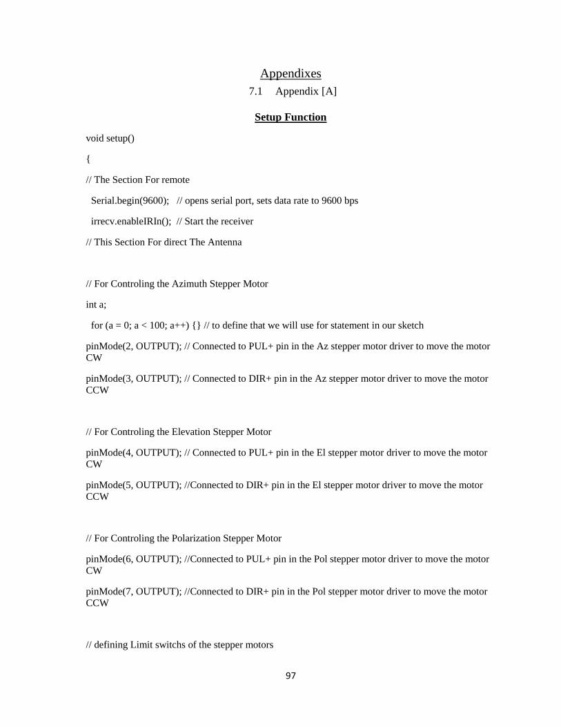
97

7 Appendixes

7.1 Appendix [A]

Setup Function

void setup()

// The Section For remote

Serial.begin(9600); // opens serial port, sets data rate to 9600 bps

irrecv.enableIRIn(); // Start the receiver

// This Section For direct The Antenna

// For Controling the Azimuth Stepper Motor

int a;

for (a = 0; a < 100; a++) // to define that we will use for statement in our sketch

pinMode(2, OUTPUT); // Connected to PUL+ pin in the Az stepper motor driver to move the motor

CW

pinMode(3, OUTPUT); // Connected to DIR+ pin in the Az stepper motor driver to move the motor

CCW

// For Controling the Elevation Stepper Motor

pinMode(4, OUTPUT); // Connected to PUL+ pin in the El stepper motor driver to move the motor

CW

pinMode(5, OUTPUT); //Connected to DIR+ pin in the El stepper motor driver to move the motor

CCW

// For Controling the Polarization Stepper Motor

pinMode(6, OUTPUT); //Connected to PUL+ pin in the Pol stepper motor driver to move the motor

CW

pinMode(7, OUTPUT); //Connected to DIR+ pin in the Pol stepper motor driver to move the motor

CCW

// defining Limit switchs of the stepper motors

98

pinMode(SW1, INPUT); // Connected to the Az Reference Point limit switch

pinMode(SW2, INPUT); // Connected to the El Reference Point limit switch

pinMode(SW3, INPUT); // Connected to the Pol Reference Point limit switch

/*---------------- (end setup ) ----------------*/

99

7.2 Appendix [B]

IR-remote encoded hexadecimal number representation sketch

The sketch that was used to display the hexadecimal number represent the IR-remote control keys

was formulated as follow:

#include <IRremote.h>

int RECV_PIN = 13;

IRrecv irrecv(RECV_PIN);

decode_results results;

void setup()

Serial.begin(9600);

irrecv.enableIRIn(); // Start the receiver

void loop()

if (irrecv.decode(andresults))

Serial.println(results.value, HEX);

irrecv.resume(); // Receive the next value

100

7.3 Appendix [C]

IR-remote Control Decoder

IRDecoder( ) // takes action based on IR code received

// Decoding IR-remote KEYES

switch(results.value)

case 0x807F807F: i=1; Serial.println(i); break;

case 0x807F40BF: i=2; Serial.println(i); break;


case 0x807F20DF: i=4; Serial.println(i); break;

case 0x807FA05F: i=5; Serial.println(i); break;

case 0x807FE01F: i=6; Serial.println(i); break;

case 0x807F10EF: i=7; Serial.println(i); break;

case 0x807F50AF: i=8; Serial.println(i); break;

case 0x807FD02F: i=9; Serial.println(i); break;


case 0x807F8877: i=777; Serial.println("EXIT"); break;

case 0x807F48B7: i=888; Serial.println(" OK "); break;

case 0x807FE817:i=9999; Serial.println(9999); break; // VOL (+)

case 0x807F28D7:i=9999; Serial.println(9999); break; // VOL (-)

case 0x807FA857:i=9999; Serial.println(9999); break; // CH (+)

case 0x807F6897:i=9999; Serial.println(9999); break; // CH (-)

case 0x807F629D:i=1004; Serial.println("FWD"); break; // FWD for skew CW

case 0x807F22DD:i=1005; Serial.println("REW"); break; // REW for skew CCW

case 0x807FE21D:i=1006; Serial.println("ResetSat"); break; // RECALL for ResetSat

101

case 0x807F00FF:i=9999; Serial.println(9999); break; // Power

case 0x807FC03F:i=9999; Serial.println(9999); break; // Mute

case 0x807F30CF:i=9999; Serial.println(9999); break; // TV/RAD

case 0x807FF00F:i=9999; Serial.println(9999); break; // TV/SAT

case 0x807F08F7:i=9999; Serial.println(9999); break; // Menu

case 0x807F18E7:i=9999; Serial.println(9999); break; // EPG

case 0x807F9867:i=9999; Serial.println(9999); break; // INFO

case 0x807FC837:i=9999; Serial.println(9999); break; // GROUP

case 0x807FF807:i=9999; Serial.println(9999); break; // COLOR

case 0x807F7887:i=9999; Serial.println(9999); break; // PAGE up

case 0x807FB04F:i=9999; Serial.println(9999); break; // PAGE down

case 0x807F58A7:i=9999; Serial.println(9999); break; // PAUSE

case 0x807F38C7:i=9999; Serial.println(9999); break; // ZOOM

case 0x807F827D:i=9999; Serial.println(9999); break; // AUDIO

case 0x807F42BD:i=9999; Serial.println(9999); break; // TEXT

case 0x807FB847:i=9999; Serial.println(9999); break; // MULTIVEIW

case 0x807FA25D:i=9999; Serial.println(9999); break; // ADVANCE

case 0x807F02FD:i=9999; Serial.println(9999); break; // REC

case 0x807F906F:i=9999; Serial.println(9999); break; // PLAY

case 0x807FD827:i=9999; Serial.println(9999); break; // STOP

case 0x807FD22D:i=9999; Serial.println(9999); break; // FILE LIST

case 0x807FC23D:i=9999; Serial.println(9999); break; // BOOK MARK

case 0x807FFA05:i=9999; Serial.println(9999); break; // SLEEP

// End Case switch

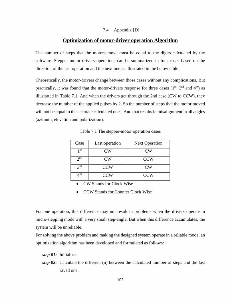
102

7.4 Appendix [D]

Optimization of motor-driver operation Algorithm

The number of steps that the motors move must be equal to the digits calculated by the

software. Stepper motor-drivers operations can be summarized in four cases based on the

direction of the last operation and the next one as illustrated in the below table.

Theoretically, the motor-drivers change between those cases without any complications. But

practically, it was found that the motor-drivers response for three cases (1st, 3rd and 4th) as

illustrated in Table 7.1. And when the drivers get through the 2nd case (CW to CCW), they

decrease the number of the applied pulses by 2. So the number of steps that the motor moved

will not be equal to the accurate calculated ones. And that results in misalignment in all angles

(azimuth, elevation and polarization).

Table 7.1 The stepper-motor operation cases

Case Last operation Next Operation

1st CW CW

2nd CW CCW

3rd CCW CW

4th CCW CCW

CW Stands for Clock Wise

CCW Stands for Counter Clock Wise

For one operation, this difference may not result in problems when the drivers operate in

micro-stepping mode with a very small step-angle. But when this difference accumulates, the

system will be unreliable.

For solving the above problem and making the designed system operate in a reliable mode, an

optimization algorithm has been developed and formulated as follows:

step 01: Initialize.

step 02: Calculate the different (n) between the calculated number of steps and the last

saved one.

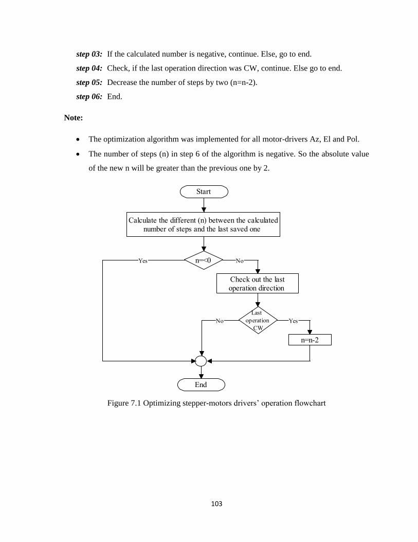
103

step 03: If the calculated number is negative, continue. Else, go to end.

step 04: Check, if the last operation direction was CW, continue. Else go to end.

step 05: Decrease the number of steps by two (n=n-2).

step 06: End.

Note:

The optimization algorithm was implemented for all motor-drivers Az, El and Pol.

The number of steps (n) in step 6 of the algorithm is negative. So the absolute value

of the new n will be greater than the previous one by 2.

Figure 7.1 Optimizing stepper-motors drivers’ operation flowchart

Start

Calculate the different (n) between the calculated number of steps and the last saved one

n=<0 NoNoYesYes

Check out the last operation direction

Last

operation

CW

NoNo YesYes

n=n-2

End

104

7.5 Appendix [E]

The specifications of the used Arduino card are as illustrated below:

ATmega32x 16 MHz Microcontroller

32 KB Flash Memory (program storage)

2 KB SRAM (program execution)

1 KB EEPROM (data storage)

14 Digital I/O Pins (6 PWM outputs)

6 Analog Input Pins

Operating Voltage 5V, 50mA

USB Interface

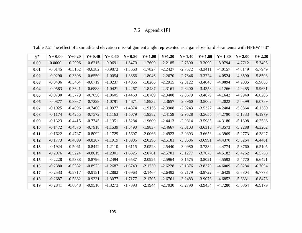
105

7.6 Appendix [F]

Table 7.2 The effect of azimuth and elevation miss-alignment angle represented as a gain-loss for dish-antenna with HPBW ≈ 3°

Y° Y+ 0.00 Y+0.20 Y+ 0.40 Y+ 0.60 Y+ 0.80 Y+ 1.00 Y+1.20 Y+ 1.40 Y+ 1.60 Y+ 1.80 Y+ 2.00 Y+ 2.20

0.00 0.0000 -0.2996 -0.6215 -0.9691 -1.3470 -1.7609 -2.2185 -2.7300 -3.3099 -3.9794 -4.7712 -5.7403

0.01 -0.0145 -0.3152 -0.6382 -0.9872 -1.3668 -1.7827 -2.2427 -2.7572 -3.3411 -4.0157 -4.8149 -5.7949

0.02 -0.0290 -0.3308 -0.6550 -1.0054 -1.3866 -1.8046 -2.2670 -2.7846 -3.3724 -4.0524 -4.8590 -5.8503

0.03 -0.0436 -0.3464 -0.6719 -1.0237 -1.4066 -1.8266 -2.2915 -2.8122 -3.4040 -4.0894 -4.9035 -5.9063

0.04 -0.0583 -0.3621 -0.6888 -1.0421 -1.4267 -1.8487 -2.3161 -2.8400 -3.4358 -4.1266 -4.9485 -5.9631

0.05 -0.0730 -0.3779 -0.7058 -1.0605 -1.4468 -1.8709 -2.3408 -2.8679 -3.4679 -4.1642 -4.9940 -6.0206

0.06 -0.0877 -0.3937 -0.7229 -1.0791 -1.4671 -1.8932 -2.3657 -2.8960 -3.5002 -4.2022 -5.0399 -6.0789

0.07 -0.1025 -0.4096 -0.7400 -1.0977 -1.4874 -1.9156 -2.3908 -2.9243 -3.5327 -4.2404 -5.0864 -6.1380

0.08 -0.1174 -0.4255 -0.7572 -1.1163 -1.5079 -1.9382 -2.4159 -2.9528 -3.5655 -4.2790 -5.1333 -6.1979

0.09 -0.1323 -0.4415 -0.7745 -1.1351 -1.5284 -1.9609 -2.4413 -2.9814 -3.5985 -4.3180 -5.1808 -6.2586

0.10 -0.1472 -0.4576 -0.7918 -1.1539 -1.5490 -1.9837 -2.4667 -3.0103 -3.6318 -4.3573 -5.2288 -6.3202

0.11 -0.1622 -0.4737 -0.8092 -1.1729 -1.5697 -2.0066 -2.4923 -3.0393 -3.6653 -4.3969 -5.2773 -6.3827

0.12 -0.1773 -0.4899 -0.8267 -1.1919 -1.5906 -2.0296 -2.5181 -3.0686 -3.6991 -4.4370 -5.3264 -6.4461

0.13 -0.1924 -0.5061 -0.8442 -1.2110 -1.6115 -2.0528 -2.5440 -3.0980 -3.7332 -4.4774 -5.3760 -6.5105

0.14 -0.2076 -0.5224 -0.8619 -1.2301 -1.6325 -2.0761 -2.5701 -3.1277 -3.7675 -4.5182 -5.4262 -6.5758

0.15 -0.2228 -0.5388 -0.8796 -1.2494 -1.6537 -2.0995 -2.5964 -3.1575 -3.8021 -4.5593 -5.4770 -6.6421

0.16 -0.2380 -0.5552 -0.8973 -1.2687 -1.6749 -2.1230 -2.6228 -3.1876 -3.8370 -4.6009 -5.5284 -6.7094

0.17 -0.2533 -0.5717 -0.9151 -1.2882 -1.6963 -2.1467 -2.6493 -3.2179 -3.8722 -4.6428 -5.5804 -6.7778

0.18 -0.2687 -0.5882 -0.9331 -1.3077 -1.7177 -2.1705 -2.6761 -3.2483 -3.9076 -4.6852 -5.6331 -6.8473

0.19 -0.2841 -0.6048 -0.9510 -1.3273 -1.7393 -2.1944 -2.7030 -3.2790 -3.9434 -4.7280 -5.6864 -6.9179

106

A Design of Automatic Dish-Antenna Positioning System for ...

Documents