A Depth-Optimal Canonical Form for Single-qubit Quantum Circuits

A Depth-Optimal Canonical Form for Single-qubit Quantum Circuits

Alex Bocharov and Krysta M. SvoreQuantum Architectures and Computation GroupMicrosoft Research, Redmond, WA 98052 USA

(Dated: June 15, 2012)

Given an arbitrary single-qubit operation, an important task is to efficiently decompose thisoperation into an (exact or approximate) sequence of fault-tolerant quantum operations. We derivea depth-optimal canonical form for single-qubit quantum circuits, and the corresponding rules forexactly reducing an arbitrary single-qubit circuit to this canonical form. We focus on the single-qubit universal {H,T} basis due to its role in fault-tolerant quantum computing, and show how ourformalism might be extended to other universal bases. We then extend our canonical representationto the family of Solovay-Kitaev decomposition algorithms, in order to find an ε-approximation to thesingle-qubit circuit in polylogarithmic time. For a given single-qubit operation, we find significantlylower-depth ε-approximation circuits than previous state-of-the-art implementations. In addition,the implementation of our algorithm requires significantly fewer resources, in terms of computationmemory, than previous approaches.

I. INTRODUCTION

Quantum algorithms assume the ability to perform anyquantum operation, however a scalable quantum com-puter will likely require the compilation of an arbitraryquantum operation into a discrete set of fault-tolerant op-erations. Various methods of decomposing an arbitraryquantum gate into a sequence of gates drawn from a uni-versal, discrete set are known [1], and typically requirefirst decomposing the operation into controlled single-qubit unitaries [2], and then decomposing the single-qubit unitaries into a circuit of gates from a universalbasis [3–5]. Given that the Steane code [6] and the sur-face code [7] yield high error thresholds, we choose todecompose into the basis containing the Hadamard op-eration (H) and the π/8 rotation (T ), {H,T}, since bothgates can be implemented fault-tolerantly in these codes.

Decomposing into a discrete gate set rarely results inan exactly equivalent unitary; the resulting sequence ismore often an ε-approximation to the original unitary. Inboth cases, it is crucial for the quantum gate decomposi-tion algorithm to minimize the circuit resources, such asthe circuit depth, the number of gates of a certain type,or the number of qubits. Since the cost of implementinga non-Clifford gate fault-tolerantly is higher than in thecase of a Clifford gate, we choose to minimize the numberof non-Clifford T gates. We call the corresponding costthe T -count of the sequence. Our approach simultane-ously minimizes circuit depth.

The Solovay-Kitaev theorem [4] states that for any εand single-qubit gate U , there exists a discrete approx-imation to U with precision ε using Θ(logc(1/ε)) gatesdrawn from the universal, discrete gate set, where c isa small constant. A constructive proof of the Solovay-Kitaev theorem was shown by Dawson et al. [8] andgives an algorithm to find an ε-approximation in timeO(log2.71(1/ε)). The resulting gate sequence has depthlogarithmic in precision ε.

Optimizing a given cost, such as the T -count, be-comes especially important in the context of the Dawson-

Nielsen algorithm [8]. The algorithm begins with a baseapproximation and then proceeds recursively, resultingin a circuit composed of O(5n) base circuits, where n isthe recursion depth. The precision of the resulting cir-cuit heavily depends on the precision of the base “0-level”circuits; if a base circuit has suboptimal cost, then thisinefficiency is amplified upon composition. In addition,the cost of a composition is often smaller than the sum ofthe costs of the factors (sub-additive); a resulting circuitcan often be compressed into a circuit with lower cost,even if the constituent factors are already optimal.

One technique for finding a better base circuit is givenby Fowler [9]. His algorithm uses previously computedknowledge of equivalent subcircuits to find a depth-optimal ε-approximation to a single-qubit gate, and runsin exponential time (and much faster than brute-forcesearch). Our canonical form algorithm does not requirecostly uniqueness checks and is relatively parsimoniousin the number of canonical circuits it generates.

Amy et al. [10] describe an algorithm for decompos-ing an n-qubit unitary into an exactly equivalent depth-

optimal circuit in time O(d |B|d/2), where d is the depthof the circuit and B is the basis. The technique is basedon a meet-in-the-middle algorithm and may be asymp-totically better than Fowler’s algorithm when determin-ing exact sequences. Their approach can also be usedfor multi-qubit circuit decomposition. We note that forsingle-qubit circuits, our canonical form algorithm can beused to find an exact decomposition, if it exists, in im-

proved time complexity O(d |B|d/4), where B = {H,T}.In this paper, we derive a canonical form for single-

qubit unitaries. A similar representation was given byMatsumoto and Amano [11], who develop a normal formfor {H,T}-circuits, where two circuits in normal formcompute the same unitary matrix if and only if the twocircuits are syntactically identical [12]. The first key dif-ference between our canonical form and the normal formin [11] is that their form is expressed in SU(2), whichcontains a non-trivial two-element center that makes thealgebra sensitive to the sign of the global phase; in con-

arX

iv:1

206.

3223

v1 [

quan

t-ph

] 1

4 Ju

n 20

12

2

trast, our canonical representation of circuits over the{H,T} basis is developed using group identities in theprojective special unitary group PSU(2). By factoringout the global phase and working in PSU(2), we are ableto further compress normal circuits. The second key dif-ference is our concept of canonical circuit , which is aunique representative of a double coset of circuits withrespect to the Clifford group. It allows further compres-sion of the depth of a circuit by writing a circuit in thecanonical form g1.c.g2, where g1, g2 are Clifford gates andc is a uniquely defined canonical circuit. Throughout, weuse . to represent circuit composition.

Our primary contributions are:

1. We present a single-qubit canonical form and cor-responding rules for reducing a single-qubit circuitinto the canonical form (Sec. II).

2. We develop an algorithm for finding an ex-act, depth-optimal decomposition of a single-qubit unitary, if it exists, else a depth-optimal ε-approximation (Sec. III).

3. We develop an efficient storage database of canon-ical circuits and an efficient search procedure overthe database (Sec. IV).

4. We develop an algorithm for finding an ε-approximation to a single-qubit unitary in polylog-arithmic time (Sec. V).

We begin by describing our canonical form and the cor-responding reduction rules.

II. A CANONICAL FORM AND CANONICALREDUCTION OF CIRCUITS

We start with PSU(2) representations of theHadamard gate H and the π/8-gate T :

H =

[i/√

2 i/√

2

i/√

2 −i/√

2

], T =

[e−iπ/8 0

0 e+iπ/8

].

The Phase gate S = T 2 and the Hadamard gate H to-gether generate a 24-element subgroup in PSU(2), whichis isomorphic to the to classical Coxeter group A3 andisomorphic to the 4-element symmetric group S4. Wedenote this group as C.

We introduce the following two circuits, each composedof two gates, and we call these basic circuits syllables:TH = T.H, and SH = S.H. In PSU(2), syllable THis a group element of infinite order (see Sec. 4.5.3 in[13]), whereas syllable SH is a group element of order3: SH.SH.SH = (SH)3 = 1.

Consider the set of all circuits generated by variouscompositions of TH and SH. We note that the basis{TH, SH} is an equivalent universal single-qubit basisto {H,T} since the following identities hold:

H = TH(SH)2TH;T = (TH)2(SH)2TH.

Throughout, we use {·} to indicate the basis elements ofa group and 〈·〉 to indicate the group generated by thoseelements.

We further note that because SH is a syllable of order3, any circuit in 〈TH, SH〉 can be immediately reducedto one where each SH-dependent subsequence is eitherSH or (SH)2. We also observe that any 〈TH, SH〉 cir-cuit with (SH)2 anywhere in the interior immediatelycollapses to an equivalent one with smaller TH count.After reducing all of the powers of SH to 0, 1, or 2,any occurrence of (SH)2 in the interior of a circuit hasthe TH syllables on both sides and thus is a part of aTH(SH)2TH pattern that collapses to H upon removalof two TH syllables. Unless this residual H is on the leftend of the reduced circuit, it further cancels with the Hof the preceding TH or SH. Intuitively, (SH)2 shouldnot occur in a well-formed circuit. In fact, we find thateven single occurrences of SH can be, in a sense, furthersqueezed out of the initial sequence of a circuit, leadingto the notion of a canonical form.

Definition. A non-empty circuit in 〈TH, SH〉 is said tobe normalized if it ends with TH and does not explic-itly contain (SH)2. A normalized circuit is either theidentity I or a non-empty normalized circuit.

In other words, a normalized circuit is either the iden-tity I or follows one of the two patterns: c.TH orc.SHTH, where c is a shorter normalized circuit.

Definition. A normalized circuit is said to be canonicalif it does not contain SH earlier than the fifth syllable.

There are only six canonical circuits with fewer thansix syllables: I, TH, (TH)2, (TH)3, (TH)4, (TH)5. Theshortest canonical circuit that contains the SH syllableis (TH)4SH.TH.

Proposition 1. Each 〈H,T 〉 circuit U can be efficientlyrepresented as either U = c.g or U = H.c.g, where c is anormalized circuit and g ∈ C.

Proposition 2. Each 〈H,T 〉 circuit U can be efficientlyrepresented as U = g1.c.g2, where c is a canonical circuitand g1, g2 ∈ C.

Thus the right C-coset of an arbitrary 〈H,T 〉 circuit Ucontains either c or H.c, where c is a normalized circuitthat can be efficiently identified, and the double C-cosetof U contains a canonical circuit that can be efficientlyidentified.

We now introduce the T -count cost and the corre-sponding trace level:

Definition. The T -count of a normalized circuit is thenumber of TH syllables in that circuit.

Definition. A trace level Lt corresponding to a value t,where 0 ≤ t ≤ 2, is the set

Lt = {U ∈ PSU(2)∣∣∣|tr(U)| = t}.

3

T -count is an invariant of the gate represented by acanonical circuit, which follows from:

Theorem 1. If c1, c2 are C-equivalent canonical circuits,i.e., ∃g1, g2 ∈ C such that c2 and g1.c1.g2 evaluate tothe same gate in PSU(2), then c1 and c2 are equal as〈TH, SH〉 circuits.

The proof of Theorem 1 is given in Appendix E.Note that in our proposed canonical form, the T -

count and and the overall circuit depth are closely tied,e.g., with a {H,T} canonical form there are at leastT -count − 1 and at most T -count + 1 Clifford gates inthe representation, and all but at most two of these gatesare either H or HSH (the number of HSH sequences isguaranteed to be less than T -count− 3).

III. DEPTH-OPTIMAL CIRCUITDECOMPOSITION

A natural technique (e.g, Fowler [9]) for finding adepth-optimal ε-approximation of U is to incrementallybuild a database containing unique quantum gates andtheir depth-optimal (shortest length) circuit representa-tion, and then for a given target gate U , perform a prox-imity search in the database. Such a database of uniquegates is expensive to build, store, and search.

In contrast, a database of canonical circuits can bebuilt without recursion and requires less memory for stor-age, allowing significantly longer (canonical) circuits tobe maintained in practice. The following remarkableobservation leads to a more efficient algorithm (thanbrute-force search and [9]) for finding a depth-optimalε-approximation:

Corollary 1. Given a single-qubit gate U ∈ PSU(2),U can be ε-approximated with an 〈H,T 〉 circuit withT -count < t if and only if one of the gates in the double

coset C.U.C = {g1.U.g2∣∣∣g1, g2 ∈ C} can be ε-approximated

by a canonical circuit with T -count < t.

It follows that the optimal ε-approximation of U un-der a certain T -count t is immediately derived from theoptimal ε-approximation of some gate G ∈ C.U.C underT -count t.

The search for metric neighbors of target gate U , wherethe measure is trace distance, in a database of all uniquegates is then replaced by a search for metric neighbors ofall elements of the C.U.C coset in the database of canoni-cal circuits. We note that there are at most 24×24 = 576elements in this coset and all of the searches can be donein parallel. The design of a scalable circuit look-up so-lution based on the canonical representation is discussedin more detail in the next section.

Fowler has compiled the multiplication table for thegroup C generated by H and S = T 2 (see Appendix A1in [9]); here we use the same notation for the group ele-ments. The H,S representations of these elements can be

found in Appendix A. Effective normalization of circuitsrelies on commutation relations between elements of Cand the T gate. There are three types of relations, estab-lished by direct computation in PSU(2) and cataloguedin Appendix B: (1) g1.T = T, g2, (2) g1.T = H.T.g2, (3)g1.T = HSH.T.g2, where g1, g2 ∈ C.

In order to work constructively with normalized andcanonical circuits, we prove the following propositions:

Proposition 3. The cost of finding a normalized repre-sentation U = c.g or U = H.c.g of an 〈H,T 〉 circuit Uis linear in the size of the circuit.

The proof of Propositions 1 and 3 is based on the actualnormalization algorithm presented in Appendix C.

Proposition 4. The cost of finding a canonical repre-sentation g1.c.g2 of an 〈H,T 〉 circuit U is quadratic inthe T -count of its normalization in the worst case.

We prove Propositions 2 and 4 in Appendix D.The inverse of a non-empty normalized circuit is not a

normalized circuit. However, its special form is describedin the following proposition:

Proposition 5. Normalized representation of the in-verse c−1 of a normalized circuit c is either of the fromH.c′.H or of the form H.c′.H.S3, where c′ is a normal-ized circuit computable in time linear in the depth of c.

Canonical circuits are parsimonious in terms of re-source requirements on a classical computer. There are2t−3 + 4 canonical circuits with T -count t or less; for ex-ample, at t = 24 the cardinality is 2, 097, 156 and theefficient lookup tree used to experiment with circuits ofthis size has a memory footprint of approximately 900MB. A classical database of canonical circuits can be usedfor many practical applications, including algorithms forperforming Solovay-Kitaev decomposition [8]. We de-scribe the classical database and how to search it effi-ciently in Section IV.

IV. SEARCH FOR CANONICALAPPROXIMATIONS

Let B = {b1, b2, ..., bk} ⊂ PSU(2). We say that B is abasis with Clifford reduction if there is a proper subset CC(to represent “Canonical Circuits”) of the subgroup 〈B〉of all of the circuits in basis B and a computable mappingCr : 〈B〉 → CC where ∀U ∈ 〈B〉, ∃g1, g2 ∈ C such thatU = g1.Cr(U).g2.

We also assume that there is a partial function

cost : 〈B〉 → Z+

that is (1) well-defined on CC; (2) zero on C; and(3) subadditive w.r.t. composition, i.e., cost(U1.U2) ≤cost(U1) + cost(U2) (whenever both the left-hand sideand the right-hand side are well-defined). We may addi-tionally assume that the cost function is strictly additiveon CC.

4

Our findings below apply to any such basis, eventhough the implicit focus of this section is on the {H,T}basis with the T -count as the target cost function. Con-sider the ε-approximation of a target gate U ∈ PSU(2)to precision ε > 0. Given a classical database of somecircuits in the basis B, the database query of primaryinterest is to find the minimum cost ε-approximation ofU :

Query 1. Find arg minv∈〈B〉(cost(V )∣∣∣dist(V,U) < ε).

Suppose now that we only have a database of some cir-cuits in the subset CC. The hypothetical approximatingcircuit V can be represented as h1.Cr(V ).h2, h1, h2 ∈ C.The cost(h1.Cr(V ).h2) ≤ cost(Cr(V )), by the assumedproperties of the cost function. We also have thatdist(h1.Cr(V ).h2, U) = dist(CR(V ), h−11 Uh−12 ).

We can now rewrite the query as

Query 2. Find

arg ming1,g2∈C,c∈CC

(cost(c)∣∣∣dist(c, g1.U.g2) < ε).

Consider the adjoint action of C on PSU(2):

Adg[U ] = g.U.g−1, g ∈ C, U ∈ PSU(2).

Since g1.U.g2 = g1.U.(g2.g1).g−11 = Adg1 [U.(g2.g1)], thequery can again be rewritten as:

Query 3. Find

arg ming,h∈C,c∈CC

(cost(c)∣∣∣dist(c, Adg[U.h]) < ε),

which is equivalent to

Query 4. Find

arg minh∈C

( ming∈C,c∈CC

(cost(c)∣∣∣dist(c, Adg[U.h]) < ε).

The final query above is scalable because the adjointaction Adg preserves the absolute matrix trace, whereasthe right action U → U.h tends to change the absolutematrix trace (for non-trivial elements of C). Thus the set

{U.h∣∣∣h ∈ C} tends to be distributed across several (up to

|C| = 24) trace levels.We use the absolute matrix trace as the primary key

in our database of CC circuits. We also assume that theproximity of two circuits implies the proximity of theirabsolute matrix trace values. This is obviously true whenthe distance measure is given by

dist(U, V ) =√

(2− |tr(U.V †|)/2,

where dist(U, V ) < ε implies that ||tr(U)|−|tr(V )|| < 4ε.Throughout, we assume this distance measure, althoughother distance measures are possible.

Now consider the list of distinct absolute trace val-

ues {t1, ..., tr} =⋃{|tr|U.h|

∣∣∣, h ∈ C} appearing in Query

4. When ε is small enough, the individual approxima-tion targets Adg[U.h], h ∈ C are distributed across non-

intersecting neighborhoods {U∣∣∣||tr(U)| − ti| < δ}, for

i = 1, . . . , r and some suitable δ > 0.Thus given that the database of the CC circuits is dis-

tributed across logical computational nodes indexed bythe absolute trace values, we have a good mapping ofapproximation target cases Adg[U.h], h ∈ C across r non-intersecting logical computational node groups.

Before describing ways of further partitioning thesearch space, we make the following empirical observa-tions:

1. Canonical circuits with T -count ≤ k have onlyO(2k/2) distinct absolute trace values (empirical es-timate: ≤ 6× 2k/2 trace values).

2. Each trace level Lt has either zero or at mostO(2k/2) canonical circuits with the T -count k.(Whenever Conjecture 1 of Sec. VII holds, the T -count is constant on trace level Lt).

3. The complexity of a search for the ε-approximationin the database of all canonical circuits with T -count ≤ k is O(εk2k) when the desired approxi-mation exists; the non-existence of the approxima-tion is discovered in O(k) steps on average and inO(k2k/2) steps in the worst case.

Now we explore the geometry of an individual trace

level Lt = {V∣∣∣|tr(V )| = t}. Except for the extreme val-

ues t = 0 and t = 2, this trace level has the geometryof a 2-dimensional Euclidean sphere with the adjoint ac-tion of the C faithful and isomorphic to the action ofthe group of symmetries of the octahedron with vertices(±1, 0, 0), (0,±1, 0), (0, 0,±1). The trace level Lt, viewedas the Euclidean sphere, can be covered with 24 funda-mental tiles of this action. For instance, we can selectthe spherical triangle F0 with vertices at x = y = 0,y = z = 0, and x = y = z, x > 0, z > 0 and generate alltiles as Adg[F0], g ∈ C. Now, consider an arbitrary fixedh ∈ C and the trace level {|tr(V )| = |tr(U.h)|} viewed asa the tiled sphere with the C tiling introduced above. Forthe majority of matrices U.h, the individual approxima-tion targets Adg[U.h], g ∈ C are distributed across differ-ent fundamental tiles.

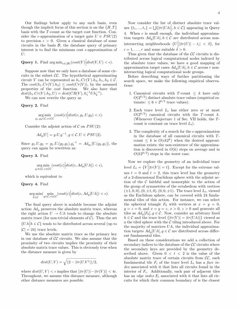
Based on these considerations we add a collection ofsecondary indices to the database of the CC circuits wherethe secondary keys are provided by the geometry de-scribed above. Given 0 < t < 2 is the value of theabsolute matrix trace of certain circuits from CC, eachfundamental tile Fi of the trace level Lt has a face in-dex associated with it that lists all circuits found in theinterior of Fi. Additionally, each pair of adjacent tileshas an edge index Ei associated with it that lists all cir-cuits for which their common boundary of is the closest

5

F0

F1

F2

F3

F13

V 0

V1

V2

V6

V5

E0

E1

E2

E3

FIG. 1. Trace level with 5 (out of 24) tiles and 6 (out of 14)vertices showing. Ei, Fi, Vi indicate edge, face, and vertexindices, respectively.

such boundary. Finally, we note 14 special points calledvertices on the trace level Lt that are meeting points ofmore than two tiles (see Figure 1). Each vertex ν has avertex index Vi associated with it that lists all circuits inLt for which ν is the closest vertex.

Consider the target U.h of the subquery of Query 4:

ming∈C,c∈CC

(cost(c)∣∣∣dist(c, Adg[U.h])) < ε.

Let 0 < t < 2, such that ||tr(U.h)| − t| < 4ε and tracelevel Lt contains some circuits from CC. For the ma-jority of matrices U , the projection of U.h on the tracelevel Lt, with high probability, is far enough from bound-aries of the fundamental tile F to the interior of whichthat projection belongs. Therefore in order to find theminc∈CC(cost(c)|dist(c, U.h)) < ε) in this case it suf-fices to inspect the face index of that tile. For a non-trivial g ∈ C the situation is isometric, so the search forminc∈CC(cost(c)|dist(c, Adg[U.h])) < ε) can be limited tothe interior of the Adg[F ] tile.

Of course with lower probability, U.h will fall withinε of some edge or vertex of the trace level Lt, whichrequires the use of multiple tile, edge or vertex indices. Inpractice the above subquery should be distributed overall relevant secondary indices. With high probability,most of the indices will be immediately eliminated basedon the trace-level geometry.

V. APPLICATION TO SOLOVAY-KITAEVDECOMPOSITION

In this section, we use our canonical representations forSolovay-Kitaev decomposition. Recall that the Dawson-Nielsen (D-N) algorithm for the Solovaty-Kitaev theorem[8] is recursive, and finer approximations require greater

recursion depth. At depth level 0, D-N returns an extrin-sic “basic” approximation of a requested single-qubit gateU . At depth n, it composes an approximation from thedepth n−1 approximation Un−1 and the depth n−1 ap-proximations of two auxiliary matrices Vn−1 and Wn−1,such that the resulting approximation is given by

Un = Vn−1.Wn−1.V†n−1.W

†n−1.Un−1. (1)

We want to maintain the canonical form for each of theapproximating circuits at each depth level, starting withbase level n = 0. We can efficiently lookup the 0-levelapproximations by using our design for efficient parallellookup over a large database of canonical circuits (seeSection IV). This results in an interesting tradeoff. Whenall 0-level approximations are sought in a database ofcanonical circuits with T -count ≤ t, where t is relativelylarge, in the worst case the D-N n-level recursion mayresult in a circuit with T -count cost O(t5n), seeminglyworsening the T -count vs. precision performance curvefor the algorithm.

On the other hand, improving the quality of the 0-level approximation may in fact decrease the requiredrecursion depth and exponentially decrease the circuit’sT -count. For example, increasing the 0-level databasescope from T -count ≤ 12 to T -count ≤ 28 improves theprecision of the 0-level approximation by a factor of 9.8 onaverage. According to the D-N estimate (Sec. 3, Eq 1 in[8]), this results in an improvement in precision by a coef-ficient around 10−6 at depth 4 and around 10−9 at depth6. Thus if we have an ε-approximation using a databasecontaining circuits with T -count ≤ 12, then we can ex-pect to have a significantly more precise ε-approximationby expanding the database to include circuits with T -counts in the high 20’s.

In practice, we find that our technique scales even bet-ter than the D-N estimate suggests. With a databaseof 0-level approximations up to T -count = 25 or 26, weare limited as early as recursion depth 4 only by the ac-curacy of the machine-defined double type. Therefore,our experimental results only cover recursion depths ≤ 3[14]. In terms of circuit cost, we barely exceed a T -count of 3000 for the longest of our circuit approxima-tions, whereas previous approaches cite T -counts of 105

or more.The impact of the canonical reduction on the quality

of the D-N commutant formula (Eq 1) is profound. Con-sider first the composition of a canonical presentationwith a normalized presentation (in this order). With-out loss of generality, we can consider composition in theform U = (g1.V.TH.g2).[H.].W.g3), where g1, g2, g3 ∈ C,W is normalized, and V.TH is canonical. The [·] indi-cates that the sequence is present in one case and ab-sent in the other. We are especially interested in caseswhere cancelation occurs, namely the resulting composi-tion has T -count smaller than the sum of the T -countsof V.TH and W . Cancelation is triggered by a certainstructure of the normalization of the (H.g2.[H.].W ) cir-cuit that is of the form W ′ = [H.][SH.]W1.g4, where

6

g4 ∈ C and the normalized circuit W1 is either emptyor starts and ends with TH. By Lemma 1, the trailingT in g1.V.T will not cancel when W ′ starts with H orSH, or when W1 is empty. Consider the remaining case:W ′ = TH.W2.g4. Here, U = g1.V.SH.W2.g4, implyingthat T -count(U) < T -count(V ) + T -count(W ).

Further transformations are necessary when V =V2.SH. If W2 starts with SH, i.e., W2 = SH.W3, thenU = g1.V2.W3.g4 is a normalized form and no furtherreduction in T -count is possible. However, if W2 startswith TH we get the infamous TH.(SH)2.TH pattern,which reduces to H, which is likely to cascade into fur-ther cancelations.

To summarize, normalized composition of circuits re-duces the T -count of the resulting circuit in many cases.An additional benefit is that by using canonical reduc-tion, we can restrict the number of Clifford gates as well.Each interior gate in a normalized circuit is either H orHSH (and if the circuit is canonical then the number ofHSH gates cannot be greater than T -count− 5).

Given an ε-approximation circuit c of a target gate U ,for example by using D-N, the normalized form of cir-cuit c, denoted by n(c), is a minimal cost circuit that isexactly equivalent to c; however, normalization does notguarantee that the result is a lowest cost ε-approximationof U . Indeed, there are potentially many normalized cir-cuits in the ε-neighborhood of U , including some withT -counts lower than the T -count of n(c), that are sim-ply not obtainable by a specific method (e.g., the D-Nalgorithm for Solovay-Kitaev).

VI. EXPERIMENTAL RESULTS

We evaluate the performance of our canonical formand reduction techniques in two experimental scenar-ios. In each case, we evaluate the performance of de-composing 10, 000 randomly generated, single-qubit uni-taries into their ε-approximations. First, we study thetradeoffs between T -count cost and precision ε for the0-level ε-approximation, employing our canonical circuitdatabase. Second, we study the same tradeoffs for the n-level ε-approximation, where n ≤ 3, using our database,canonical reduction, and the recursive Solovay-Kitaev al-gorithm [8].

To evaluate our findings, we generated and cata-logued each of the 268, 435, 460 canonical circuits withT -count ≤ 31. Our database of canonical circuits hasthe absolute matrix trace as its primary index, and hassecondary indices based on the fundamental tiles of theadjoint representation of the C group (see Sec. IV).

Our experiments and database required a memoryfootprint of 120GB and the use of a high-performancemulti-core workstation. We discovered, however, thatcanonical circuits with T -count > 25 did not offer signif-icant improvements in T -count/precision ε tradeoffs inthe second experimental scenario using machine doubleaccuracy. In practice, a database of canonical circuits of

0.0005

0.005

0.05

5 10 15 20 25 30 35

Pre

cisi

on

ϵ

T-count

Canonical lookup Fowler lookup

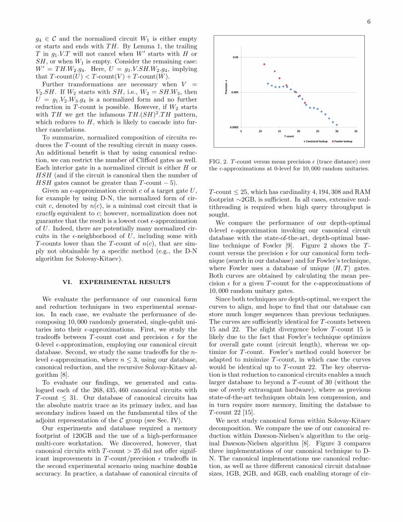
FIG. 2. T -count versus mean precision ε (trace distance) overthe ε-approximations at 0-level for 10, 000 random unitaries.

T -count ≤ 25, which has cardinality 4, 194, 308 and RAMfootprint ∼2GB, is sufficient. In all cases, extensive mul-tithreading is required when high query throughput issought.

We compare the performance of our depth-optimal0-level ε-approximation invoking our canonical circuitdatabase with the state-of-the-art, depth-optimal base-line technique of Fowler [9]. Figure 2 shows the T -count versus the precision ε for our canonical form tech-nique (search in our database) and for Fowler’s technique,where Fowler uses a database of unique 〈H,T 〉 gates.Both curves are obtained by calculating the mean pre-cision ε for a given T -count for the ε-approximations of10, 000 random unitary gates.

Since both techniques are depth-optimal, we expect thecurves to align, and hope to find that our database canstore much longer sequences than previous techniques.The curves are sufficiently identical for T -counts between15 and 22. The slight divergence below T -count 15 islikely due to the fact that Fowler’s technique optimizesfor overall gate count (circuit length), whereas we op-timize for T -count. Fowler’s method could however beadapted to minimize T -count, in which case the curveswould be identical up to T -count 22. The key observa-tion is that reduction to canonical circuits enables a muchlarger database to beyond a T -count of 30 (without theuse of overly extravagant hardware), where as previousstate-of-the-art techniques obtain less compression, andin turn require more memory, limiting the database toT -count 22 [15].

We next study canonical forms within Solovay-Kitaevdecomposition. We compare the use of our canonical re-duction within Dawson-Nielsen’s algorithm to the orig-inal Dawson-Nielsen algorithm [8]. Figure 3 comparesthree implementations of our canonical technique to D-N. The canonical implementations use canonical reduc-tion, as well as three different canonical circuit databasesizes, 1GB, 2GB, and 4GB, each enabling storage of cir-

7

1E-08

0.0000001

0.000001

0.00001

0.0001

0.001

0.01

0.1

10 100 1000 10000 100000

Pre

cisi

on

ϵ

T-count

SK+4G lookup SK+1G lookup Dawson code SK+2G lookup

FIG. 3. T -count versus mean precision ε (trace distance) overthe ε-approximations at n-level recursion for 10, 000 randomunitaries and n = 0, 1, 2, 3, where the markers indicate therecursion level n.

cuits with up to T -count 24, 25, and 26, respectively.Each curve represents the mean precision ε for a givenT -count for the ε-approximations of 10, 000 random uni-tary gates for recursion levels n = 0, 1, 2, 3. Both axes inthe graph are plotted on the logarithmic scale.

First, we note that there is no visible difference be-tween the 2GB canonical implementation and the 4GBcanonical implementation. Second, we observe that ourtechnique, for all three implementations, is able to find,for a given ε, approximations with significantly smaller T -count. In particular, at T -counts below 500, our methodsachieve ε = 5 × 10−8, offering a factor of 10−6 improve-ment over D-N. To improve the precision of our techniqueeven further, it would require computation of the matrixtrace using precision beyond the limit of machine doubleprecision. At the best D-N precision of ε = 5×10−5, D-Nrequires roughly 100, 000 T gates on average, while our2GB implementation (SK+2G) requires only 120 T gates

on average (a factor of 846 improvement).

VII. CONCLUSIONS AND FUTURE WORK

We have defined a depth-optimal canonical form andcorresponding reduction rules for single-qubit quantumcircuits. Our techniques result in significant improve-ments in terms of database size and achieved precisionin the case of the depth-optimal 0-level ε-approximation,and significant improvements in the T -count/precision εcurve when applied to Solovay-Kitaev decomposition forn-levels of recursion. A natural future direction is to gen-eralize the definition of a canonical form to multi-qubitgates as well as to other universal bases.

Another direction is to perform “lossy compression”,where the task is to find an approximately equivalentcircuit (within distance ε of the target gate) that requiresless cost, in terms of a given cost function such as T -count or number of gates. We believe such a solution itwill require the following conjecture:

Conjecture 1. If c1, c2 are canonical circuits andT -count(c1) 6= T -count(c2) then |tr(c1)| 6= |tr(c2)|.

This conjecture implies that if a trace level Lt = {U ∈PSU(2)

∣∣∣|tr(U)| = t} contains multiple canonical circuits,

all of these circuits have the same T -count. We currentlyhave only empirical brute-force evidence of Conjecture 1for T -count ≤ 31.

ACKNOWLEDGMENTS

We thank Dave Wecker, Burton Smith, Michael Freed-man, Zhenghan Wang and John Platt for useful discus-sions. We also wish to thank Rodney Van Meter andNathan Cody Jones for sharing the benchmark D-N al-gorithm data with us.

[1] P. O. Boykin, T. Mor, M. Pulver, V. Roychowdhury, andF. Vatan, http://arxiv.org/abs/quant-ph/9906054(1999), URL http://arxiv.org/abs/quant-ph/

9906054.[2] A. Barenco, C. Bennett, R. Cleve, D. DiVincenzo,

N. Margolus, P. Shor, T. Sleator, J. Smolin, and H. We-infurter, Phys. Rev. A 52 (1995).

[3] A. Kitaev, Russian Math. Surveys 52, 1191 (1997).[4] A. Kitaev, A. Shen, and M. Vyalyi, Classical and

Quantum Computation (American Mathematical Soci-ety, Providence, RI, 2002).

[5] N. C. Jones, J. D. Whitfield, P. L. McMahon, M. Yung,R. van Meter, A. Aspuru-Guzik, and Y. Yamamoto(2012), URL http://arxiv.org/abs/1204.0567v1.

[6] P. Aliferis, D. Gottesman, and J. Preskill, Quantum In-formation and Computation 6, 97 (2006), URL http:

//arxiv.org/abs/quant-ph/0504218.[7] A. G. Fowler, A. M. Stephens, and P. Groszkowski,

Phys. Rev. A 80 (2009), URL http://arxiv.org/abs/

quant-ph/0803.0272.[8] C. Dawson and M. Nielsen, Quantum Information and

Computation 6, 81 (2006), URL http://arxiv.org/

abs/quant-ph/0505030.[9] A. Fowler, Ph.D. thesis, Univ. of Melbourne (2005), URL

http://arxiv.org/abs/quant-ph/0506126.[10] M. Amy, D. Maslov, M. Mosca, and M. Roetteler (2012),

URL http://arxiv.org/abs/1206.0758.[11] K. Matsumoto and K. Amano (2008), URL http://

arxiv.org/abs/0806.3834.[12] Note1, our work was developed independently; we were

made aware of this work while writing our paper.[13] M.A.Nielsen and I.L.Chuang, Quantum Computation

8

and Quantum Information (Cambridge University Press,Cambridge, UK, 2000).

[14] Note2, finer analysis would seem to require extendedfloating point precision.

[15] Note3, note that each increase by 1 in T -count requiresroughly twice the amount of memory.

Appendix A: Elements of the C group

The following definitions are equivalent to the onesgiven in (Appendix A1 in [9]).

G0 = Id;G1 = H;G2 = HSSH;G3 = SS;G4 = S;G5 = SSS;G6 = HSS;G7 = SSH;G8 = SH;G9 = SSSH;G10 = SSHSSH;G11 = SHSSH;G12 = SSSHSSH;G13 = HS;G14 = HSSS;G15 = SSHSS;G16 = SHSS;G17 = SSSHSS;G18 = HSH;G19 = HSSSH;G20 = HSHSSH;

G21 = HSSSHSSH;G22 = SSSHS;G23 = SHSSS

Appendix B: C/T commutation relations

G1.T = H.T ;G2.T = T.G12;G3.T = T.G3;G4.T = T.G4;G5.T = T.G5;G6.T = H.T.G3;

G7.T = H.T.G12;G8.T = H.SH.T.G2;G9.T = H.SH.T.G4;G10.T = T.G11;G11.T = T.G2;G12.T = T.G10;

G13.T = H.T.G4;G14.T = H.T.G5;G15.T = H.T.G11;G16.T = H.SH.T.G10;G17.T = H.SH.T.G5;G18.T = H.SH.T ;G19.T = H.SH.T.G12;G20.T = H.T.G2;G21.T = H.T.G10;G22.T = H.SH.T.G3;

G23.T = H.SH.T.G11

Appendix C: Proof of Propositions 1 and 3

Since T 2 = S ∈ C, any 〈H,T 〉 circuit has the form

U = (∏ki=1 gi.T ).g, k ≥ 0, where g, gi ∈ C, gi 6= Id when

i > 1.Collect all factors in this product (in the order they

appear) into a gateList. The following algorithm is tail-recursive, and group C is denoted by C:

Algorithm

CircuitNormalize(input: gateList):gateList =if gateList is empty thenreturn empty list

let left <- {head(input)}let right <- tail(input)while (left is not empty) &&

(right is not empty) doif head(right) = T thenif head(left) = T thenleft <- tail(left)

right <- {G4} + tail(right)// G4=S=T.T

else // head(left) in Cif head(left) = H[SH] thenleft <- {T} + leftright <- tail(right)

elselet cmt <- //see Appendix 2apply C/T commutationtable to head(left) and T

left <- tail(left)if (cmt = H[SH].T.g , g in C)thenleft <- { g, T, H[SH]} + leftright <- tail(right)

else if (cmt = T.g , g in C)thenright <- { T, g} + right

elseif head(left) = T thenleft <-{head(right)} + left

else // head(left), head(right) in Clet g <- C product of

head(left) and head(right)left <- tail(left)if g <> Id thenleft = {g} + left

right <- tail(right)if left is empty then

return CircuitNormalize(right)else

return reverse(left) + right

The intent of this algorithm is to eliminate all of theClifford gates that are different from either H or HSHfrom the interior of the “gateList”. The cost of each suchelimination is bound by a constant. Thus the cost of thealgorithm is linear in terms of the number of such Cliffordgates and hence linear in terms of the length of the inputcircuit.

Appendix D: Proof of Propositions 2 and 4

Lemma 1. A normalized circuit of the form U =SHTH.c (where c is a normalized subcircuit) canbe effectively rewritten as a normalized representationH.SHTH.c1.g, g ∈ C with the number of rewrites linearin the T -count of c. The resulting circuit c1 has the sameT -count as c.

Proof. By brute force, we establish that SHTH =HSHT.HSS and “upset” the normalization to start withHSHT.HSS.c. The rest of the proof is similar to theproof of Propositions 1 and 3, i.e., we establish by linearinduction that HSS.c reduces to H.c1.g, g ∈ C, where c1is a normalized circuit.

Informally, if a normalized circuit starts with SH then

9

we can force it into a normalized presentation that startswith H.

We are now ready to prove Propositions 2 and 4.

Proof. Let U = [H.]c.g be a normalized representation ofa given U ∈ PSU(2). Note that c may start with theSH syllable, in which case, we split it off. Now considerU = [H.][SH.]c.g, where c is a normalized circuits start-ing with the TH syllable. Further proof is based on thefollowing identities that can be established by brute-forcecalculation in PSU(2):

THSHT = G2.THT.G4;THTHSHT = G3.THTHT.G2;THSHTHT = G10.THTHT.G11;THSHTHSHT = G2.THTHT.G5;

THTHTHSHT = G11.THTHTHT.G4;THTHSHTHT = G5.THTHTHT.G11;THSHTHTHT = G4.THTHTHT.G12;THTHSHTHSHT = G3.THTHTHT.G5;THSHTHSHTHT = G5.THTHTHT.G3;THSHTHTHSHT = G10.THTHTHT.G10;THSHTHSHTHSHT = G2.THTHTHT.G2;

Informally, these are used to “squeeze” SH sylla-bles out of the first four syllables of c into surround-ing C factors. If c has fewer than five TH syllables,we immediately obtain U = g1.c

′.g2, g1, g2 ∈ C, wherec′ is a canonical circuit. We now assume that c hasT -count t > 4 and that the propositions have beenproven for all T -counts smaller than t. Consider theshortest prefix of the circuit c spanned by its leftmostfour TH syllables and apply one of the above trans-formation rules to that prefix, thus obtaining reductionof the form U = g1.THTHTHT.g

′.c′.g, g1, g′, g ∈ C,

where c′ is a normalized circuit. Apply Proposition 1to subcircuit g′.c′.g to obtain a normalized presentationV = [H.][SH.]c′′.g′′, g′′ ∈ C, where c′′ is a normalizedcircuit that is either empty or starts with TH. In theempty case c′′, we trivially get the canonical presenta-tion U = g1.THTHTHTH.(H.[H.][SH.]g

′′). Otherwise,we need to consider the following three cases:

1. V starts with H. This yields canonical presentationU = g1.THTHTHTH.[SH.]c

′′.g′′;

2. V starts with SH, as per Lemma 1 we can force itto start with H and reduce to the first case.

3. V starts with TH, i.e., V = TH.c′′′.g′′,hence U = g1.THTHTHT.TH.c

′′′.g′′ =g1.THTHT.HSH.c

′′′.g′′, where THTHTHSH.c′′′

is normalized with T -count smaller than t. Thelatter is not canonical, since there is the SHoccurring earlier than the fifth syllable, howeverthe circuit is normalized with T -count smallerthan t and can be recursively brought to canonicalform as per the induction hypothesis.

Note that the last case is the only one responsible forthe potentially quadratic cost of the canonical reduction.

Normalization of subcircuits of the above g′.c′.g form haslinear cost. For the overall cost to become quadratic, thecircuit shape as in clause 3 must occur O(t) times in theat most t/2 recurring rewrites, which is fairly unlikely.In fact, in practice we have never seen clause 3 invokedin our experiments.

Appendix E: Proof of Theorem 1

We outline a proof by induction of Theorem 1. It isreminiscent of Sec. 4.2 in [11], albeit dramatically simplerand shorter.

Proof. The simple initial step is to note that if there existsuch g1, g2, c1, c2 that c2 = g1.c1.g2 as matrices and c2 6=c1 as circuits then there exists a normalized circuit n,with T -count(n) > 0, that evaluates to a matrix in C.Since SH ∈ C and T -count(SH) = 0, n, without loss ofgenerality, starts with TH.

Now consider the adjoint action of PSU(2) on its Liealgebra L = su(2), adu[m] = u.m.u†, u ∈ PSU(2), m ∈L. It is a well known fact that L consists of zero-traceHermitian matrices and is spanned over R by the Paulimatrices X,Y, Z.

The adjoint action of the C subgroup on L is thesymmetry group of the octahedron with vertices at±X,±Y,±Z. In particular, for each g ∈ C, adg[Z] mustbe one of these vertices. To obtain a contradiction itsuffices to show that for a normalized circuit n, adn(Z)cannot be in {±X,±Y,±Z}.

Let A ∈ L be a matrix over Q(√

2) represented as:

(√

2)lA = (x0 +x1√

2)X+ (y0 +y1√

2)Y + (z0 + z1√

2)Z,

where x0, x1, y0, y1, z0, z1 are integers.

We show that if A = adn(Z) then (1) x0 is odd and(2) y0, z0 have the opposite parity. The (1) implies thatthe coefficient at X is non-zero and the (2) implies thatat least one other coefficient (at Y or at Z) is non-zero;together they imply that adn(Z) cannot be proportionalto any one Pauli matrix.

We prove the desired properties (1) and (2) by induc-tion on the T -count of n. By direct computation:

adTH(X) = Z,

adTH(Y ) = (X − Y )/√

2,

adTH(Z) = (X + Y )/√

2,

adSHTH(X) = Y,

adSHTH(Y ) = (−X + Z)/√

2,

adSHTH(Z) = (X + Z)/√

2,

and, in particular, properties (1) and (2) hold for

adTH(Z) = (X + Y )/√

2 ( x0 = 1, y0 = 1, z0 = 0 ).

10

Given matrix A ∈ L presented as shown above, wehave:

(√

2)l+1adTH(A) = ((y0 + z0) + (y1 + z1)√

2)X +

((z0 − y0) + (z1 − y1)√

2)Y + (2x1 + x0√

2)Z,

(√

2)l+1adSHTH(A) = ((z0 − y0) + (z1 − y1)√

2)X +

(2x1 + x0√

2)Y + ((y0 + z0) + (y1 + z1)√

2)Z.

By induction hypothesis, y0, z0 have opposite parity,therefore the new x0 that is equal to either y0+z0 or z0−y0 is odd in both cases. In the expression for adTH(A),the new y′0 = z0−y0 is odd but the new z′0 = 2x1 is even.In the expression for adSHTH(A), the new y′0 = 2x1 iseven but the new z′0 = y0 + z0 is odd.

Since each non-trivial normalized circuit is eithern1.TH or n1.SHTH, where n1 is a shorter normalizedcircuit, this concludes the inductive proof.