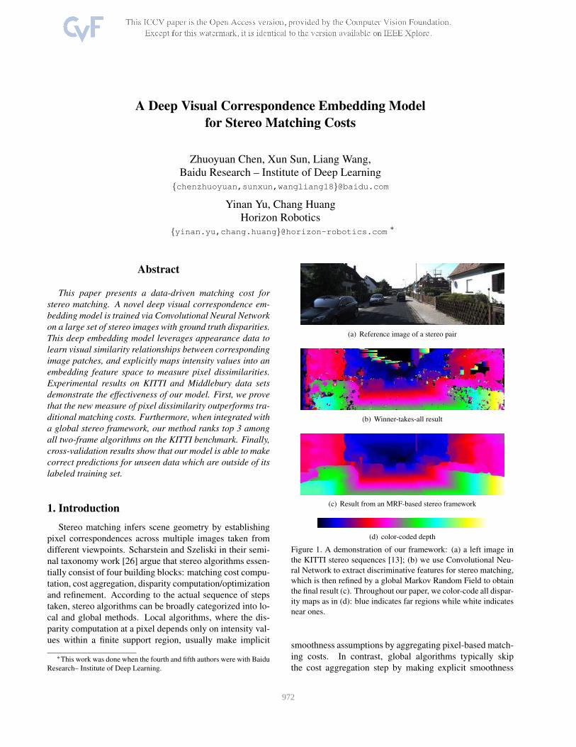
A Deep Visual Correspondence Embedding Model for … · A Deep Visual Correspondence Embedding Model for Stereo Matching Costs Zhuoyuan Chen, Xun Sun, Liang Wang, Baidu Research –

A Deep Visual Correspondence Embedding Model

for Stereo Matching Costs

Zhuoyuan Chen, Xun Sun, Liang Wang,

Baidu Research – Institute of Deep Learning

{chenzhuoyuan,sunxun,wangliang18}@baidu.com

Yinan Yu, Chang Huang

Horizon Robotics

{yinan.yu,chang.huang}@horizon-robotics.com ∗

Abstract

This paper presents a data-driven matching cost for

stereo matching. A novel deep visual correspondence em-

bedding model is trained via Convolutional Neural Network

on a large set of stereo images with ground truth disparities.

This deep embedding model leverages appearance data to

learn visual similarity relationships between corresponding

image patches, and explicitly maps intensity values into an

embedding feature space to measure pixel dissimilarities.

Experimental results on KITTI and Middlebury data sets

demonstrate the effectiveness of our model. First, we prove

that the new measure of pixel dissimilarity outperforms tra-

ditional matching costs. Furthermore, when integrated with

a global stereo framework, our method ranks top 3 among

all two-frame algorithms on the KITTI benchmark. Finally,

cross-validation results show that our model is able to make

correct predictions for unseen data which are outside of its

labeled training set.

1. Introduction

Stereo matching infers scene geometry by establishing

pixel correspondences across multiple images taken from

different viewpoints. Scharstein and Szeliski in their semi-

nal taxonomy work [26] argue that stereo algorithms essen-

tially consist of four building blocks: matching cost compu-

tation, cost aggregation, disparity computation/optimization

and refinement. According to the actual sequence of steps

taken, stereo algorithms can be broadly categorized into lo-

cal and global methods. Local algorithms, where the dis-

parity computation at a pixel depends only on intensity val-

ues within a finite support region, usually make implicit

∗This work was done when the fourth and fifth authors were with Baidu

Research– Institute of Deep Learning.

(a) Reference image of a stereo pair

(b) Winner-takes-all result

(c) Result from an MRF-based stereo framework

(d) color-coded depth

Figure 1. A demonstration of our framework: (a) a left image in

the KITTI stereo sequences [13]; (b) we use Convolutional Neu-

ral Network to extract discriminative features for stereo matching,

which is then refined by a global Markov Random Field to obtain

the final result (c). Throughout our paper, we color-code all dispar-

ity maps as in (d): blue indicates far regions while white indicates

near ones.

smoothness assumptions by aggregating pixel-based match-

ing costs. In contrast, global algorithms typically skip

the cost aggregation step by making explicit smoothness

1972

assumptions and seek an optimal disparity assignment by

solving an MRF (Markov Random Field) based energy op-

timization problem.

Matching cost computation, as a fundamental step

shared by both local and global stereo algorithms, plays an

important role in establishing visual correspondences. Typi-

cally, the reconstruction accuracy of a stereo method largely

depends on the dissimilarity measurement of image patches.

However, the visual correspondence search problem is dif-

ficult due to matching ambiguities, which generally results

from sensor noise, image sampling, lighting variations, tex-

tureless or repetitive regions, occlusions, etc.

In this paper, we focus on the matching cost computa-

tion step and present a data-driven approach to address am-

biguities. Inspired by the recent advances in deep learn-

ing, a new deep visual correspondence embedding model

is trained via Convolutional Neural Network on a large set

of stereo images with ground truth disparities. This deep

embedding model leverages appearance data to learn visual

dissimilarity between image patches, by explicitly mapping

raw intensity into a rich embedding space. Quantitative

evaluations with ground truth data demonstrate the effec-

tiveness of our learned deep embedding model for dissim-

ilarity computation. It is first proved that the proposed

measure of pixel dissimilarity outperforms some widely

used matching costs such as sampling-insensitive absolute

differences [1], absolute differences of gradient, normal-

ized cross-correlation and census transform [41] for local

window-based matching. Furthermore, we incorporate our

learning-based matching costs with a semi-global method

(SGM) [16] and show that our model matches state-of-the-

art performance on the KITTI stereo data set [13] for accu-

racy while being superior to other top performers for effi-

ciency and simplicity. Lastly, our deep embedding model

is evaluated on the Middlebury benchmark [25] to quan-

titatively assess its capability of generalization. Cross-

validation results show that our model is able to make cor-

rect predictions across stereo images outside of its labeled

training set.

1.1. Previous Work

Stereo has been a highly active research topic of com-

puter vision for decades and this paper owes a lot to a siz-

able body of literature on stereo matching, more than we

hope to account for here. For the scope of this paper, our

focus is on the matching costs computation step and we re-

fer interested readers to [18, 34, 26] for more detailed de-

scriptions and evaluations of different components of stereo

algorithms.

Common pixel-based matching costs include absolute

differences (AD), squared differences (SD) and sampling-

insensitive differences (BT) [1]. In practice, truncated

versions of these methods are usually adopted because of

the robustness brought about by the cost aggregation and

global optimization steps. Common window-based match-

ing costs include normalized cross-correlation (NCC), sum

of absolute or squared differences (SAD/SSD), gradient-

based measures, and non-parametric measures such as rank

and census transforms [41]. Methods such as BT, SAD

and SSD are built strictly on the brightness constancy as-

sumption while gradient-based and non-parametric mea-

sures are more robust to radiometric changes (e.g., due to

gain and exposure differences) or non-Lambertian surfaces

at the cost of lower discriminative power. Recently, self-

adapting dissimilarity measures that combine SAD, Census

and gradient-based measures are employed by some state-

of-the-art stereo algorithms [19, 4, 39].

CNN (Convolutional Neural Networks) dates back

decades in the machine learning community [21] and de-

veloped rapidly in recent years, thanks to the advances in

learning models [23], larger data sets, and parallel comput-

ing devices, as well as the access to many online resources

[6, 27]. CNN makes breakthroughs in various computer vi-

sion tasks such as image classification [20, 32], object de-

tection [14, 10], face recognition [33, 30], and image pars-

ing [11]. Besides its success in high-level vision appli-

cations, deep learning also shows its capability in solving

certain low-level vision tasks such as super-resolution [7],

denoising [2], and single-view depth estimation [8].

Our work is closely related to a recent paper [35], in

which CNN is leveraged to compute stereo matching costs.

In comparison to [35], our deep embedding model differs

from [35] in two main aspects: 1) Given the feature vec-

tors (corresponding to the left right patches in a stereo pair)

output by CNN, we directly compute their similarity in the

Euclidean space by a dot product. In contrast, the archi-

tecture in [35] is more complicated, in that feature vectors

requires further fully-connected DNN (Deep Neural Net-

work) to obtain the final similarity score in a non-Euclidean

space. The architecture of our CNN leads to two orders of

magnitude (100×) speed-up in computing a dense disparity

map compared to [35] with little sacrifice in reconstruction

accuracy. 2) Our embedding model is learned from a multi-

scale ensemble framework, which automatically fuses fea-

tures vectors learned at different scale-space. Deep learn-

ing is also applied in [12, 22] for feature matching. How-

ever, [12] extracts features at sparse locations while [22]

targets at matching semantically similar regions. Our model

is also related to the Deep Flow model [37], where convo-

lutional matching is applied to estimate optical flow. The

difference is that [37] applies bottom-up deep dynamic pro-

gramming on hand-crafted HOG features, while our model

is data-driven and learned.

2973

Le#$

image$

patch$

L1$ L2$ L3$ L4$

Share

Share

core1

L1$ L2$ L3$ L4$

L1$ L2$ L3$ L4$

Share Share

Share

core2

L1$ L2$ L3$ L4$

Share

Right$

image$

patch$

1x1x2 voting

Figure 2. The network architecture of our training model for deep embedding. Features are extracted in a pair of patches at different scales,

followed by an inner product to obtain the matching scores. The scores from different scales are then merged for an ensemble.

2. Deep Embedding for Stereo Estimation

Given a pair of rectified left/right images {IL, IR}, a

typical stereo algorithm begins by computing the matching

quality: denoting patches IL(p) and IR(p − d) centered

at pL = (x, y) and pRd = (x − d, y), we generate match-

ing score S(p,d) = f(IL(p), IR(p− d)) for each p with

different disparity d = (d, 0). The score serves as an im-

portant initialization, generally followed by a non-local re-

finement such as cost aggregation or filtering [24, 42]. In

this section, we focus on our data-driven model to learn a

good matching quality measure.

2.1. Multi-scale Deep Embedding Model

Consider a pair of patches IL(p), IR(p − d) of size

13 × 13, we propose to learn an embedding model to

extract features f(I), such that the inner-product S =<

f(IL(p)), f(IR(p−d)) > tends to be large in case of posi-

tive matching and small for negative ones. This differs from

the binary classification model in [35].

Multi-Scale Embedding: we apply an ensemble model

[11, 5, 8] in our deep embedding, which largely improves

the matching quality. Denoting IL↓ (p), IR↓ (p−d) as patches

at the coarse scale, we have:

S(p,d) = w1 < f(IL(p), f(IR(p− d)) > +

w2 < f(IL↓ (p), f(IR↓ (p− d) >

As we know, the choice of patch scale and size is very

tricky: large patches with richer information are less am-

biguous, but more risky of containing multiple objects and

producing blurred boundaries; small patches have merits in

motion details, but are very noisy. Accordingly, we propose

a weighted ensemble of two scales to combine the best of

two worlds.

Our embedding framework is shown in Figure 2. The

inputs are two pairs of 13 × 13 × 1 image patches, cen-

tered at p = (x, y), p − d = (x − d, y) with two differ-

ent scales. The blue-colored dash box indicates the orig-

inal resolution while the red is a ×2 down-sampling. We

apply a 4-layer CNN model to extract features f(I), fol-

lowed by an inner-product layer to calculate the matching

score < f(IL), f(IR) > and an ensemble voting. Layer

L1 and L2 contain c1 = c2 = 32 kernels of size 3 × 3;

Layer L3 and L4 contain kernels c3 = c4 = 200 of size

5 × 5. At both scales, the weights in all layers L1...L4 for

left and right patches are tied. Then, features f4(I) ∈ R200

undergo inner-product operations, outputting two scalars

S1 =< f4(IL), f4(I

R) > and S2 =< f4(IL↓ ), f4(I

R↓ ) >

as matching scores. Finally, S1 and S2 are merged by a

1× 1× 2 convolutional layer for a weighted ensemble.

In our training process, we apply a deep regression

model and minimize the Euclidean cost:

E(w) = ||S(p,d)− label(p,d)||2 (1)

where label(p,d) = {0, 1} indicates whether pL = (x, y)corresponds to p− d = (x− d, y) in the right image. Rec-

tified linear units [23] follow each layer, but we do not use

pooling to preserve spatial-variance.

3974

Figure 3. The deployed network architecture of our testing model

for deep embedding. Features are extracted in two images only

once respectively. Then, the sliding-window style inner product

can be grouped for matrix operation.

2.2. Efficient Embedding for Testing

With deep embedding, we achieve 100× speedup at test

time compared to MC-CNN [35]. We attribute this to the

largely shared computation in the forward pass as well as

grouped matrix operation.

The insight is shown in Figure 3, we extract features

f4(I) in each image only once with a fully convolutional

neural network, and then the matching score S(p,d) is

computed with all potential offsets d by the sliding-window

style inner product. In comparison, in [35] the fully-

connected layers require recomputation every time when d

is varied.

Moreover, multiple inner product operations can be

grouped together as a matrix operation for further accelera-

tion. That is, we multiply f(IL(p)) with the matrix F (IR),whose columns contain features f(IR(p− d)) with differ-

ent d. This matrix multiplication is highly parallel in nature.

2.3. Training Details

A training example comprises two pairs of patches

{IL(p), IR(p−d)}, {IL↓ (p), IR↓ (p−d)}. We sample pos-

itive and negative examples at ratio 1 : 1 at each location

where the disparity d is known. A negative example is ob-

tained by shifting the right patch to pd = (x−d+oneg, y),where oneg ∈ {−Nhi, ...,−Nlo, Nlo, ..., Nhi} is a random

corrupting offset. Similarly, positive examples are pd =(x− d+ opos, y), with opos ∈ {−Phi, Phi}.

In practice, we find that a warm start with large Nlo, Nhi

makes the training converges faster. We gradually decrease

Nlo, Nhi to pursue a hard negative mining.

3. Stereo Framework

To calculate the final disparity map using our proposed

matching costs, we adopt an MRF-based stereo framework.

First of all, a cost volume is initialized by negating our deep

embedding scores as C(p, d) = −S(p, pd).

Secondly, the initial costs are then fed to the semi-global

matcher (SGM) [16, 39] to compute a raw disparity map.

Thirdly, after removing unreliable matches via a left-right

check, the final disparity map is obtained by propagating

reliable disparities to non-reliable areas [29]. In the fol-

lowing, we will briefly summarize the key building blocks

in our framework.

Formulating the stereo problem as an MRF model, the

SGM aims to find a disparity assignment D that minimizes:

E(D) =X

p

(C(p, d) +X

q∈N(p)

P1[|d−Dq| = 1]

+X

q∈N(p)

P2[|d−Dq| > 1])(2)

The constant parameters P1 and P2 penalize disparity dis-

continuity and P1 < P2. While an exact solution to equa-

tion (2) is NP-hard, semi-global matcher obtains an ap-

proximation by performing multiple dynamic programming

(DP)-style 1D cost updates along multiple directions as

Lr(p, d) =C(p, d) + min(Lr(p− r, d),

Lr(p− r, d± 1) + P1,

mini(Lr(p− r, i) + P2))

(3)

where Lr(p, d) is the cost along a direction r. After averag-

ing the costs along 16 directions, the initial disparity map is

computed for left and right views by picking the disparity

hypothesis with the minimal cost.

To efficiently remove the remaining outliers in the initial

disparity map, we adopt a propagation scheme [29, 40]. We

start by performing a left-right consistency check to roughly

divide all pixels into stable and unstable sets. Assuming that

a stable pixel p should satisfy DLeft(p) = DRight(p− d),we carry out a propagation on the cost volume as:

C(p, d)pro =

⇢

|d−DLeftRaw (p)|2 p is stable,

0 else.(4)

Here for stable pixels, we penalize disparity deviation from

its initial disparity values. In contrast, for unstable pixels,

the costs are set to zero for all disparity hypotheses. Thus,

an edge-aware filter applied on this cost volume leads to re-

liable disparity propagation in the cost domain. We choose

the O(1) geodesic filter derived from a tree structure [29]

due to its effectiveness and efficiency. After filtering the

propagated cost volume C(p, d)pro, we again choose the

disparity assignment using winner-takes-all. Finally, we

employ a 3 × 3 median filter to remove remaining isolated

noises.

4975

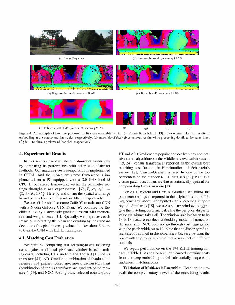
(a) Image Sequence (b) Low-resolution d↓, accuracy 94.2%

(c) High-resolution d, accuracy 89.6% (d) Ensemble d∗, accuracy 95.8%

(e) Refined result of d∗ (Section 3), accuracy 98.5% (f) (g) (h) (i)

Figure 4. An example of how the proposed multi-scale ensemble works. (a) Frame 10 in KITTI [13]; (b,c) winner-takes-all results of

embedding at the coarse and fine scales, respectively; (d) ensemble of (b,c) gives smooth results while preserving details at the same time;

(f,g,h,i) are close-up views of (b,c,d,e), respectively.

4. Experimental Results

In this section, we evaluate our algorithm extensively

by comparing its performance with other state-of-the-art

methods. Our matching costs computation is implemented

in CUDA. And the subsequent stereo framework is im-

plemented on a PC equipped with a 3.0 GHz Intel i5

CPU. In our stereo framework, we fix the parameter set-

tings throughout our experiments: {P1, P2, σs, σr} ={5, 80, 20, 10.5}. Here σs and σr are the spatial and range

kernel parameters used in geodesic filters, respectively.

We use off-the-shelf resource Caffe [6] to train our CNN

with a Nvidia GeForce GTX Titan. We optimize the Eu-

clidean loss by a stochastic gradient descent with momen-

tum and weight decay [31]. Specially, we preprocess each

image by subtracting the mean and dividing by the standard

deviation of its pixel intensity values. It takes about 3 hours

to train the CNN with KITTI training set.

4.1. Matching Cost Evaluation

We start by comparing our learning-based matching

costs against traditional pixel and window-based match-

ing costs, including BT (Bircheld and Tomasi) [1], census

transform [41], AD+Gradient (combination of absolute dif-

ferences and gradient-based measures), Census+Gradient

(combination of census transform and gradient-based mea-

sures) [39], and NCC. Among these selected counterparts,

BT and AD+Gradient are popular choices by many compet-

itive stereo algorithms on the Middlebury evaluation system

[19, 24]; census transform is reported as the overall best

matching cost function in Hirschmuller and Scharstein’s

survey [18]; Census+Gradient is used by one of the top

performers on the outdoor KITTI data sets [39]; NCC is a

classic patch-based measure that is statistically optimal for

compensating Gaussian noise [18].

For AD+Gradient and Census+Gradient, we follow the

parameter settings as reported in the original literature [19,

39], census transform is computed with a 5×5 local support

region. Similar to [18], we use a square window to aggre-

gate the matching costs and calculate the per-pixel disparity

value via winner-takes-all. The window size is chosen to be

13 × 13 because our deep embedding model is learned on

the same size. NCC does not go through cost aggregation

with the patch width set to 13. Note that no disparity refine-

ment step is applied in this experiment because we want the

raw results to provide a more direct assessment of different

methods.

We report performance on the 194 KITTI training im-

ages in Table 1. As can be seen, our learned matching costs

from the deep embedding model substantially outperform

traditional matching costs.

Validation of Multi-scale Ensemble: Close scrutiny re-

veals the complementary power of the embedding results

5976

Figure 5. Some disparity map results using our embedding cost on KITTI benchmark. The left column: grayscale images of the left

frames; The right column: our final results. From top to bottom: different frames in the KITTI data set.

Methods All err(%) Non-occ err(%)

Multi-scale 11.1 9.5

Single-scale (Coarse) 14.8 12.7

Single-scale (Fine) 17.4 14.6

BT 37.8 36.6

Census 25.1 23.4

AD+Gradient 37.4 36.1

Census+Gradient 23.5 21.7

NCC 21.8 19.9

Table 1. Quantitative evaluation of different costs with local-

window matching. We compare errors of winner-takes-all re-

sults obtained by classical costs with our deep embedding model

(single-scale and the multi-scale ensembles) in all and non-

occluded regions.

at different scales (e.g., the 10-th frame in KITTI train-

ing set). As shown in Figure 4, the embedding at low-

resolution tends to generate more smooth results, but is at

risk of losing motion details. Thin structures like the tree

marked in box in (a) are missing in (b,f), where the lost mo-

tion proposal can hardly be recovered by post-processing.

Meanwhile, noises in high-resolution results (c) can be sup-

pressed by accounting for larger contexts. The accuracy of

ensemble (95.8%) is higher than any single scale and a post-

processing can produce satisfactory stereo results.

Quantitatively, the average accuracy of winner-takes-all

results produced by the fine-scale, coarse-scale and multi-

scale ensemble are 85.4%, 87.3% and 90.5% on the KITTI

train set, respectively.

4.2. Stereo Pipeline Evaluation

In this section, we incorporate our matching costs with

the stereo framework introduced in section 3. The quantita-

tive evaluation results on KITTI test set are shown in table

2, where we compare our model with state-of-the-art meth-

ods with only two stereo images for fairness (algorithms

that leverage multi-view or temporal/scene flow cues are

beyond the scope of this paper). Our method ranks the 3rdamong these algorithms in terms of accuracy as of Septem-

ber 2015, and is over an order of magnitude faster than [15]

and [35]. Note that replacing our deep embedding costs

6977

Method Out-Noc Out-All Avg-Noc Avg-All Runtime Environment

Displets [15] 2.47 % 3.27 % 0.7 px 0.9 px 265s 8+ cores @ 3.0 Ghz (Matlab + C/C++)

MC-CNN [35] 2.61 % 3.84 % 0.8 px 1.0 px 100s Nvidia GTX Titan (CUDA, Lua/Torch7)

Ours 3.10 % 4.24 % 0.9 px 1.1 px 3.0s Nvidia GTX Titan (CUDA, Caffe)

Census+Gradient 3.91 % 5.10 % 0.9 px 1.0 px 2.5s single core @ 3.0Ghz GPU

CoR[3] 3.30 % 4.10 % 0.8 px 0.9 px 6s 6 cores @ 3.3 Ghz (Matlab + C/C++)

SPS-St[39] 3.39% 4.41% 0.9 px 1.0 px 2s 1 core @3.5 Ghz (C/C++)

DDS-SS[36] 3.83 % 4.59 % 0.9 px 1.0 px 1 min 1 core @ 2.5 Ghz (Matlab + C/C++)

PCBP[38] 4.04 % 5.37 % 0.9 px 1.1 px 5 min 4 cores @ 2.5 Ghz (Matlab + C/C++)

CoR-Conf[3] 4.49 % 5.26 % 1.0 px 1.2 px 6 s 6 cores @ 3.3 Ghz (Matlab + C/C++)

AARBM[9] 4.86 % 5.94 % 1.0 px 1.2 px 0.25 s 1 core @ 3.0 Ghz (C/C++)

wSGM [28] 4.97 % 6.18 % 1.3 px 1.6 px 6s 1 core @ 3.5 Ghz (C/C++)

Table 2. Qualitative evaluation of our pipeline on KITTI benchmark with the error threshold set as 3 pixels. The method ”Census+Gradient”

uses the same stereo framework, but with Census+Gradient cost function rather than our proposed learning-based matching costs. In terms

of runtime, we would like to emphasize that the numbers given in this table are total running time of the whole stereo framework. As

reported in the paper [35], the MC-CNN algorithm takes about 95 seconds to compute their learning-based matching costs and 5 seconds

for semi-global matching and disparity post-processing steps. In contrast, the running time for our matching cost computation is about 1.0

second, which is around 100 times faster than [35].

with Census+Gradient [39] produces inferior results. A

few disparity maps generated by our method are presented

in Figure 5, from which we can see that our algorithm pro-

duces piecewise smooth and visually plausible results. Our

method not only preserves geometry details near depth dis-

continuities, but also performs well on challenging regions

such as textureless and shadow areas.

Regarding the running time, the CNN step takes about

1.0s on average, 734ms at the original resolution and 267ms

at the coarse resolution. This is about 100× speedup com-

pared to MC-CNN [35]. The acceleration factor mainly re-

sults from fewer model parameters (116,000 versus 600,000

in [35]), fully-convolutional architecture and grouped ma-

trix operation. The not fully optimized MRF stereo imple-

mentation takes about 2s on CPU. In total, our approach

takes about 3s to process an image at the resolution of

1242 × 376 with a large disparity searching range from 0

to 255.

4.3. Cross-Validation

It is of interest to evaluate how our model performs on

different datasets. Besides KITTI (outdoor street view), we

further test our deep embedding model on indoor scenarios

without any fine-tuning. We choose stereo sequences from

Middlebury benchmarks [25, 17], containing a total num-

ber of 27 high resolution image pairs.

Quantitatively, we compare our algorithm with tradi-

tional costs such as AD, census transform and NCC. We

evaluate the performance with varying error thresholds τ

in Figure 6: similar to the setup in section 4.1, we carry

out a box aggregation on raw costs and obtain final dispar-

ities with a winner-takes-all treatment. It is clear that our

embedding model consistently outperforms other methods.

Especially, with τ = 3, our method achieves an average er-

Figure 6. The error curve on Middlebury benchmark with varying

error thresholds.

ror rate of 13.6%, which is much lower than SAD (33.8%),

census transform (22.2%), and NCC (21.9%). This demon-

strates that our deep embedding model generalizes well on

scenes that are sufficiently different from the training data.

We provide more qualitative results in Figure 7.

5. Conclusion and Future Work

In this paper, we introduce a novel data-driven patch

dissimilarity measure for visual correspondence. We learn

a deep embedding model to extract discriminative fea-

tures from patches in stereo pairs. Our model has fewer

parameters and shallower network structures therefore is

much more efficient than a previous learning-based model

[35]. Deep embedding produces high-quality initialization,

which can be refined with an MRF-based stereo algorithm

to obtain the state-of-the-art dense disparity estimates. Our

results on KITTI [13] and Middlebury [26] benchmarks

7978

Figure 7. Examples of winner-takes-all results using our deep embedding cost on Middlebury data. From left to right: the Cloth, Dolls,

Books and Moebius Sequences in Middlebury benchmark; From top to bottom: the left images, winner-takes-all results of our deep

embedding and ground truth.

suggest that deep embedding is robust across stereo images

taken from different environment. In the future, training

with larger data sets might have potential to further im-

prove the matching accuracy. We will also accelerate the

algorithm for real-time navigation and extend our model to

solve other low-level vision problems such as optical flow.

6. Acknowledgements

We would like to thank Haoyuan Gao and Fei Qing for

their efforts in data collection. We would also like to thank

Kai Yu and Carl Case for discussion and helpful advice.

References

[1] S. Birchfield and C. Tomasi. A pixel dissimilarity measure

that is insensitive to image sampling. PAMI, 20:401–406,

1998.

[2] H. C. Burger, C. J. Schuler, and S. Harmeling. Image denois-

ing: Can plain neural networks compete with bm3d? CVPR,

pages 2392–2399, 2012.

[3] A. Chakrabarti, Y. Xiong, S. J. Gortler, and T. Zickler. Low-

level vision by consensus in a spatial hierarchy of regions.

CVPR, 2015.

[4] Z. Chen, H. Jin, Z. Lin, S. Cohen, and Y. Wu. Large dis-

placement optical flow from nearest neighbor fields. CVPR,

2013.

[5] D. Ciresan, U. Meier, and J. Schmidhuber. Multi-column

deep neural networks for image classification. CVPR, pages

3642–3649, 2012.

[6] J. Donahue, Y. Jia, O. Vinyals, J. Hoffman, N. Zhang,

E. Tzeng, and T. Darrell. Decaf: A deep convolutional acti-

vation feature for generic visual recognition. ICML, 2014.

[7] C. Dong, C. C. Loy, K. He, and X. Tang. Learning a deep

convolutional network for image super-resolution. ECCV,

2014.

[8] D. Eigen, C. Puhrsch, and R. Fergus. Depth map prediction

from a single image using a multi-scale deep network. NIPS,

pages 2366–2374, 2014.

[9] N. Einecke and J. Eggert. Block-matching stereo with re-

laxed fronto-parallel assumption. In In Intelligent Vehicles

Symposium Proceedings, 2014 IEEE, pages 700–705, 2014.

[10] D. Erhan, C. Szegedy, A. Toshev, and D. Anguelov. Scalable

object detection using deep neural networks. CVPR, 2014.

[11] C. Farabet, C. Couprie, L. Najman, and Y. LeCun. Learning

hierarchical features for scene labeling. PAMI, 35(8):1915–

1929, 2013.

[12] P. Fischer, A. Dosovitskiy, and T. Brox. Descriptor match-

ing with convolutional neural networks: a comparison to sift.

Technical Report 1405.5769, arXiv(1405.5769), 2014.

8979

[13] A. Geiger, P. Lenz, and R. Urtasun. Are we ready for au-

tonomous driving? the kitti vision benchmark suite. In

CVPR, 2012.

[14] R. Girshick, J. Donahue, T. Darrell, and J. Malik. Rich fea-

ture hierarchies for accurate object detection and semantic

segmentation. CVPR, 2014.

[15] F. Guney and A. Geiger. Displets: Resolving stereo ambigu-

ities using object knowledge. In CVPR, 2015.

[16] H. Hirschmuller. Stereo processing by semiglobal matching

and mutual information. PAMI, 30(2):328–341, 2008.

[17] H. Hirschmuller and D. Scharstein. Evaluation of cost func-

tions for stereo matching. CVPR, 2007.

[18] H. Hirschmuller and D. Scharstein. Evaluation of stereo

matching costs on images with radiometric differences.

PAMI, 31:1582–1599, 2009.

[19] A. Klaus, M. Sormann, and K. Karner. Segment-based stereo

matching using belief propagation and a self-adapting dis-

similarity measure. ICPR, 2006.

[20] A. Krizhevsky, I. Sutskever, and G. E. Hinton. Imagenet clas-

sification with deep convolutional neural networks. NIPS,

2012.

[21] Y. LeCun, L. Bottou, Y. Bengio, and P. Haffner. Gradient-

based learning applied to document recognition. Proceed-

ings of the IEEE, 86(11):2278–2324, 1998.

[22] J. Long, N. Zhang, and T. Darrell. Do convnets learn corre-

spondence? NIPS, 2014.

[23] V. Nair and G. E. Hinton. Rectified linear units improve re-

stricted boltzmann machines. ICML, 2010.

[24] C. Rhemann, A. Hosni, M. Bleyer, C. Rother, and

M. Gelautz. Fast cost-volume filtering for visual correspon-

dence and beyond. In CVPR, 2011.

[25] D. Scharstein and C. Pal. Learning conditional random fields

for stereo. CVPR, 2007.

[26] D. Scharstein and R. Szeliski. A taxonomy and evaluation of

dense two-frame stereo correspondence algorithms. IJCV,

47(1-3):7–42, 2002.

[27] P. Sermanet, D. Eigen, X. Zhang, M. Mathieu, R. Fergus,

and Y. LeCun. Overfeat: Integrated recognition, localization

and detection using convolutional networks. arXiv preprint

arXiv:1312.6229, 2013.

[28] R. Spangenberg, T. Langner, and R. Rojas. Weighted semi-

global matching and center-symmetric census transform for

robust driver assistance. In In Computer Analysis of Images

and Patterns, pages 34–41, 2013.

[29] X. Sun, X. Mei, S. Jiao, M. Zhou, Z. Liu, and H. Wang. Real-

time local stereo via edge-aware disparity propagation. PRL,

49:201–206, 2014.

[30] Y. Sun, X. Wang, and X. Tang. Deep learning face represen-

tation from predicting 10,000 classes. CVPR, 2014.

[31] I. Sutskever, J. Martens, G. Dahl, and G. Hinton. On the

importance of initialization and momentum in deep learning.

ICML, 2013.

[32] C. Szegedy, W. Liu, Y. Jia, P. Sermanet, S. Reed,

D. Anguelov, D. Erhan, V. Vanhoucke, and A. Rabinovich.

Going deeper with convolutions. arXiv:1409.4842, 2014.

[33] Y. Taigman, M. Yang, M. Ranzato, and L. Wolf. Deepface:

Closing the gap to human-level performance in face verifica-

tion. CVPR, 2014.

[34] F. Tombari, S. Mattoccia, L. D. Stefano, and E. Addimanda.

Classification and evaluation of cost aggregation methods for

stereo correspondence. CVPR, 2008.

[35] J. Zbontar and Y. LeCun. Computing the stereo matching

cost with a convolutional neural network, 2014.

[36] D. Wei, C. Liu, and W. T. Freeman. A data-driven regular-

ization model for stereo and flow. In 3D Vision (3DV), 2014

2nd International Conference on, 1:277–284, 2014.

[37] P. Weinzaepfel, J. Revaud, Z. Harchaoui, and C. Schmid.

Deepflow: Large displacement optical flow with deep match-

ing. ICCV, pages 1385–1392, 2013.

[38] K. Yamaguchi, T. Hazan, D. McAllester, and R. Urtasun.

Continuous markov random fields for robust stereo estima-

tion. In ECCV, pages 45–58, 2012.

[39] K. Yamaguchi, D. McAllester, and R. Urtasun. Efficient joint

segmentation, occlusion labeling, stereo and flow estimation.

ECCV, 2013.

[40] Q. Yang. A non-local cost aggregation method for stereo

matching. In CVPR, 2012.

[41] R. Zabih and J. Woodfill. Non-parametric local transforms

for computing visual correspondence. ECCV, 1994.

[42] K. Zhang, J. Lu, and G. Lafruit. Cross-based local stereo

matching using orthogonal integral images. IEEE Trans-

actions on Circuits and Systems for Video Technology,

19(7):1073–1079, 2009.

9980