A Deep Learning Identification, Type-3 Fuzzy Control and LMI ...

energies

Article

Frequency Regulation System: A Deep Learning Identification,Type-3 Fuzzy Control and LMI Stability Analysis

Ayman A. Aly 1, Bassem F. Felemban 1 , Ardashir Mohammadzadeh 2,*, Oscar Castillo 3

and Andrzej Bartoszewicz 4

Citation: Aly, A.A.; Felemban, B.F.;

Mohammadzadeh, A.; Castillo, O.;

Bartoszewicz, A. Frequency

Regulation System: A Deep Learning

Identification, Type-3 Fuzzy Control

and LMI Stability Analysis. Energies

2021, 14, 7801. https://doi.org/

10.3390/en14227801

Received: 21 October 2021

Accepted: 18 November 2021

Published: 22 November 2021

Publisher’s Note: MDPI stays neutral

with regard to jurisdictional claims in

published maps and institutional affil-

iations.

Copyright: © 2021 by the authors.

Licensee MDPI, Basel, Switzerland.

This article is an open access article

distributed under the terms and

conditions of the Creative Commons

Attribution (CC BY) license (https://

creativecommons.org/licenses/by/

4.0/).

1 Department of Mechanical Engineering, College of Engineering, Taif University, P.O. Box 11099,Taif 21944, Saudi Arabia; [email protected] (A.A.A.); [email protected] (B.F.F.)

2 Independent Researcher, 1148 Baku, Azerbaijan3 Division of Graduate Studies and Research, Tijuana Institute of Technology, Tijuana 22414, Mexico;

[email protected] Institute of Automatic Control, Lodz University of Technology, 18 Stefanowskiego St., 90-537 Łódz, Poland;

[email protected]* Correspondence: [email protected]

Abstract: In this paper, the problem of frequency regulation in the multi-area power systems withdemand response, energy storage system (ESS) and renewable energy generators is studied. Dis-similarly to most studies in this field, the dynamics of all units in all areas are considered to beunknown. Furthermore time-varying solar radiation, wind speed dynamics, multiple load changes,demand response (DR), and ESS are considered. A novel dynamic fractional-order model basedon restricted Boltzmann machine (RBM) and deep learning contrastive divergence (CD) algorithmis presented for online identification. The controller is designed by the dynamic estimated model,error feedback controller and interval type-3 fuzzy logic compensator (IT3-FLC). The gains of errorfeedback controller and tuning rules of the estimated dynamic model are extracted through thefractional-order stability analysis by the linear matrix inequality (LMI) approach. The superiority ofa schemed controller in contrast to the type-1 and type-2 FLCs is demonstrated in various conditions,such as time-varying wind speed, solar radiation, multiple load changes, and perturbed dynamics.

Keywords: type-3 fuzzy systems; restricted Boltzmann machine; control systems; frequency regula-tion; linear matrix inequality

1. Introduction

By developing the renewable energy systems, the problem of the load frequencycontrol (LFC) in power systems has become one of the interesting topics. Because thechanges in solar radiation, time-varying wind speed, and variation of load power are thenatural perturbation in these systems. The main controllers that frequently have beenused are classified into 3 cases: simple PID controllers, fuzzy based PID controllers, andfractional-order PID controllers. The robust controllers with guaranteed stability are seldominvestigated in literature [1–5].

In the first case, the conventional PID controller and lag-lead compensators are used.The main difference between studies is the type of optimization algorithm. For instance,in [6], the imperialist competitive optimization technique is proposed to adjust the coeffi-cients of PID control system and its regulation function is compared by the PI controlleroptimized with genetic algorithm. In [7], the optimized PID controller by a chaotic op-timization method is proposed and its effectiveness is shown by applying on two areaspower system. In [8], the capability of the genetic algorithm is examined on the PIDfrequency regulation problem. In [9], the grey wolf optimization method is developedfor designing a PID control scheme for LFC. In [10], honey bee mating method is utilizedfor obtaining the optimized gains for PID and its regulation proficiency is investigated.

Energies 2021, 14, 7801. https://doi.org/10.3390/en14227801 https://www.mdpi.com/journal/energies

Energies 2021, 14, 7801 2 of 21

The PID controller tuned by bacterial foraging method is designed in [11] for two areassystem and its efficiency is studied in contrast to the conventional PID and optimized PIDby genetic algorithm. In [12], the PID controller is tuned on basis of grey wolf method andit is shown that the regulation performance is progressed in term of peak overshoot.

In the second case, the fuzzy PID (FPID) controllers have been developed for LFC. Thefuzzy systems are one of the best approach to deal with the uncertainties [13–15]. In thiscase, commonly the type-1 fuzzy logic systems (T1-FLSs) are employed to extract the gainsof the PID control scheme and various optimization techniques specially evolutionary basedalgorithms are used for optimization of the parameters of FLSs. For example, in [16], a FPIDis designed and the big bang–big crunch algorithm is proposed for optimization. In [17],the fuzzy PI controller is generated using the bat algorithm for LFC, and its superiorityis evaluated in comparison to other similar controllers, such as conventional PID. In [18],the teaching–learning optimization algorithm is studied for designing the FPID controllerfor LFC and it is verified that the regulation performance is improved in contrast to theother optimized PID controllers. In [19], the cuckoo and harmony search algorithms aresuggested for designing the FPID controller for LFC. In [20], the multi-verse algorithmis proposed for optimization of the FPID and its proficiency is evaluated by applying ontwo-area power system. The differential evolution tuning technique is developed in [21]for optimizing the FPID controller. In [22], the robustness of the FPID controller is studiedon two areas of the photovoltaic–thermal system. In [23], the sine–cosine algorithm isused for designing FPID. In [24], the effectiveness of grey wolf algorithm is studied incomparison with the bee colony method in the designing of FPID controller for LFC. In [25],the improvement of frequency regulation of FPID controller based on the moth swarmoptimization approach is studied by providing an real-time examination.

For the third case, recently the fractional-order (FO) PID (FO-PID) control techniqueand FO fuzzy logic controllers (FLCs) are also developed for LFC [26,27]. For example,in [28], the FO-PID controller is designed on the basis of a symbiotic organisms techniqueand is applied for frequency control in a microgrid. In [29], similarly to the previouslyreviewed studies, the FO-PID controller is optimized by multi-verse method and its superi-ority is authenticated by several simulations. In [30], the frequency regulation performanceof the traditional PID is improved employing fractional-order calculus and moth flametuning method. In [31], the effectiveness of the FO control scheme is examined by applyingon single and two areas system. In [32], the FO-PID controller is improved by Salp swarmoptimization algorithm and time-delay effect is analyzed. In [33], the impact of sometime-varying factors in the dynamics of a two areas power system is taken into accountand a FO-PID is designed and it is authenticated that FO-PID is more effective.

In most of the above reviewed studies, the closed-loop stability is not investigated andalso the control system is presented for a special power system with restricted objects andareas. Furthermore, the evolutionary based optimization algorithms are utilized to adjustthe control parameters that impose a high computational cost beside of lack of stabilityguarantee. Additionally, the effect of natural disturbances, such as simultaneous changes ofthe wind speed, solar radiation, and load perturbation, are rarely studied. The robustness ofthe controller are quite seldom studied. For example in [34], the event triggered controlleris combined with the H∞ criteria to ensure the robustness of the frequency regulator.Considering the aforementioned literature review and investigation, in this study a novelintelligent frequency regulator is suggested for multi-areas power system. Dissimilarlyto the reviewed studies, the system model is online identified by the suggested dynamicfractional-order RBM. A new compensator is designed by the IT3-FLS to tackle the effect ofthe approximation error and other perturbations. The closed-loop stability is analysed byLMI approach. The main contributions of this study are:

• The dynamics of all units in all areas are considered to be unknown;• In addition to unknown dynamics, the effects of time-varying parameters, solar

radiation, wind speed, and multiple load changes are taken to account;

Energies 2021, 14, 7801 3 of 21

• A novel dynamic fractional-order model using RBMs and deep learning algorithm isproposed for online identification;

• A novel compensator on basis of IT3-FLS is presented to cope with the dynamic modelapproximation error;

• A new LMI approach is developed to derive the error feedback gains and to guaranteethe stability and robustness.

In the remain of this study, the problem is described in Section 3, the suggesteddynamic fractional-order model is described in Section 4, the proposed IT3-FLC is given inSection 5, the stability is analyzed Section 6, the simulations and conclusions are presentedin Sections 7 and 8, respectively.

2. System Description

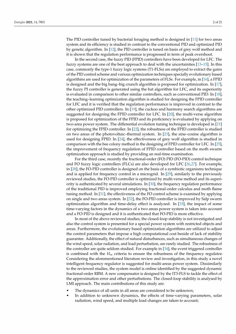
The under control plant is shown in Figure 1. The case study plant, includes, loads,photovoltaic (PVs), battery/flywheel ESS (BESS)/(FESS), micro-turbines, and wind turbine(WT). Consider the k-th area, the power changing is written as [35,36]:

Figure 1. The suggested control block diagram.

∆Pk,tie =N∑

i=1,i 6=k∆Pki,tie

= 2πs

[N∑

i=1,i 6=kTki∆ωk −

N∑

i=1,i 6=kTki∆ωi

] (1)

where, N represents number of area, ∆Pk,tie represents the power variation between tie-lineand k-th area, ∆ω is frequency deviation and Tki is torque coefficient of tie-line synchro-nization. Consider a disturbance applied to 1-th area as:

∆P1,tie =2π

s[T12∆ω1 − T12∆ω2] (2)

Then, ∆ω2 is:

∆ω2 =

(−∆P2,tie − ∆P2L +

n∑

k=1∆Pm2i

)D2 + 2H2s

(3)

Energies 2021, 14, 7801 4 of 21

Then, by applying the load disturbance into k-th area, ∆Pk,tie and ∆ωk are written as:

∆Pk,tie =2π

s

[N

∑i=1,i 6=k

Tki∆ωk

](4)

∆ωk =(−∆Pk,tie − ∆PkL)

Dk + 2Hks(5)

Considering a step perturbation in load as ∆PkL(s) = ∆PkL/s and from (5), ∆Pk,tie becomes:

∆Pk,tie =

−2π∆PkLN∑

i=1,i 6=kTki/2Hk(

s2 + Dk/2Hk + 2πN∑

i=1,i 6=kTki/2Hk

)s

(6)

The regional demand response (RDR) is implemented as follows. If d2∆Pk,tiedt2 < 0 and

d2∆Pi,tiedt2 > 0 or d2∆Pk,tie

dt2 > 0 and d2∆Pi,tiedt2 < 0, then:

RDRk = δ− d2∆Pk,tie

dt2 Hk

πN∑

i=1,i 6=kTki

(7)

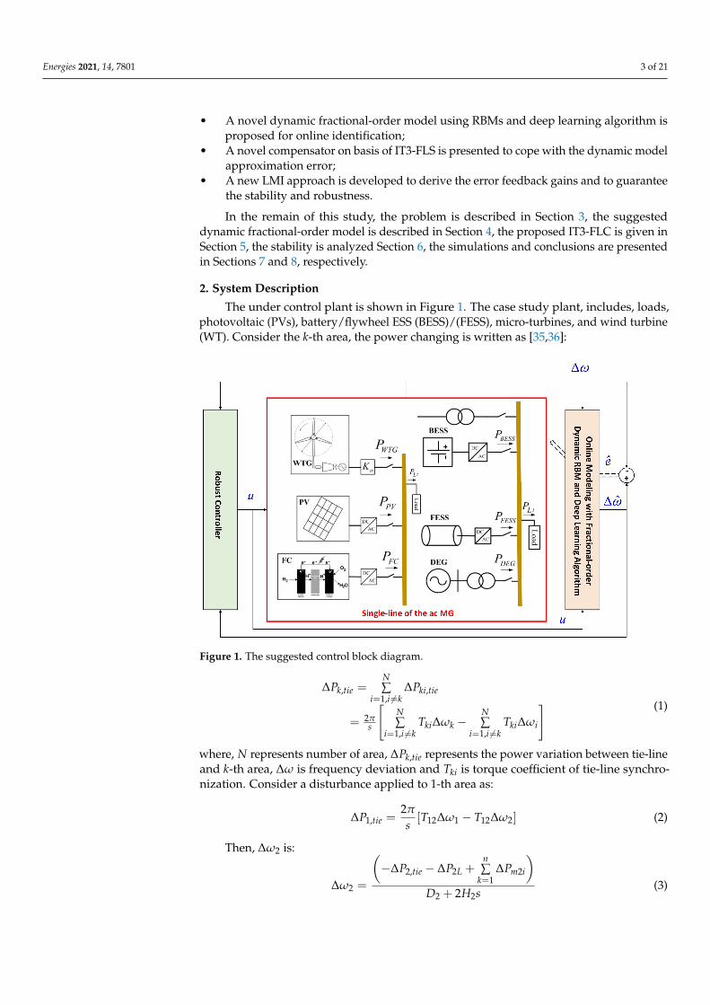
where, 0 < δ < 1. The dynamics of the other units are given in Figure 2.

Figure 2. The general diagram of case study.

Energies 2021, 14, 7801 5 of 21

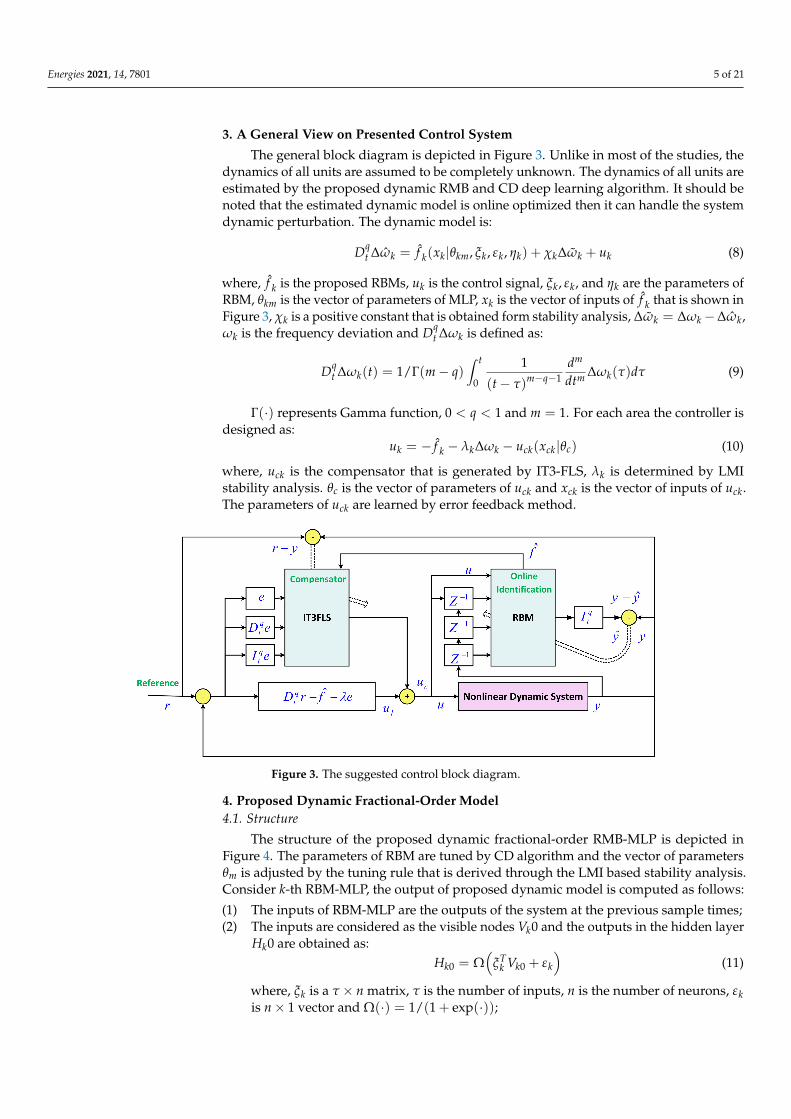
3. A General View on Presented Control System

The general block diagram is depicted in Figure 3. Unlike in most of the studies, thedynamics of all units are assumed to be completely unknown. The dynamics of all units areestimated by the proposed dynamic RMB and CD deep learning algorithm. It should benoted that the estimated dynamic model is online optimized then it can handle the systemdynamic perturbation. The dynamic model is:

Dqt ∆ωk = f k(xk|θkm, ξk, εk, ηk) + χk∆ωk + uk (8)

where, f k is the proposed RBMs, uk is the control signal, ξk, εk, and ηk are the parameters ofRBM, θkm is the vector of parameters of MLP, xk is the vector of inputs of f k that is shown inFigure 3, χk is a positive constant that is obtained form stability analysis, ∆ωk = ∆ωk−∆ωk,ωk is the frequency deviation and Dq

t ∆ωk is defined as:

Dqt ∆ωk(t) = 1/Γ(m− q)

∫ t

0

1

(t− τ)m−q−1dm

dtm ∆ωk(τ)dτ (9)

Γ(·) represents Gamma function, 0 < q < 1 and m = 1. For each area the controller isdesigned as:

uk = − f k − λk∆ωk − uck(xck|θc) (10)

where, uck is the compensator that is generated by IT3-FLS, λk is determined by LMIstability analysis. θc is the vector of parameters of uck and xck is the vector of inputs of uck.The parameters of uck are learned by error feedback method.

Figure 3. The suggested control block diagram.

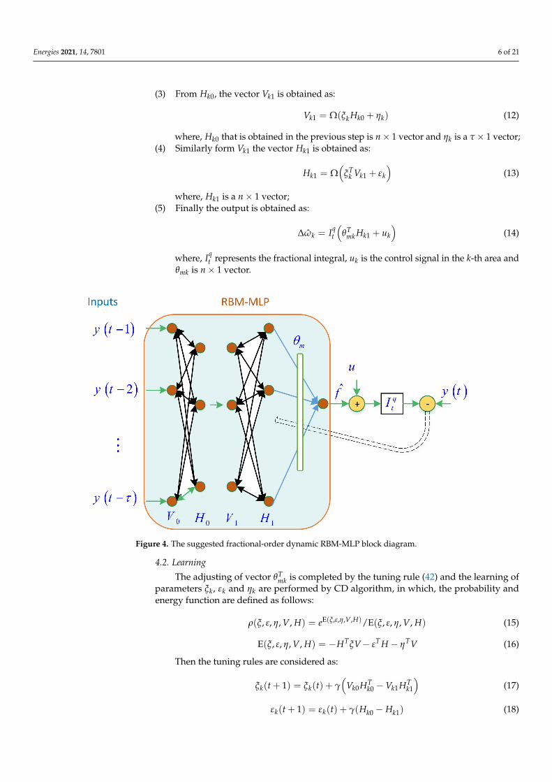
4. Proposed Dynamic Fractional-Order Model4.1. Structure

The structure of the proposed dynamic fractional-order RMB-MLP is depicted inFigure 4. The parameters of RBM are tuned by CD algorithm and the vector of parametersθm is adjusted by the tuning rule that is derived through the LMI based stability analysis.Consider k-th RBM-MLP, the output of proposed dynamic model is computed as follows:

(1) The inputs of RBM-MLP are the outputs of the system at the previous sample times;(2) The inputs are considered as the visible nodes Vk0 and the outputs in the hidden layer

Hk0 are obtained as:Hk0 = Ω

(ξT

k Vk0 + εk

)(11)

where, ξk is a τ × n matrix, τ is the number of inputs, n is the number of neurons, εkis n× 1 vector and Ω(·) = 1/(1 + exp(·));

Energies 2021, 14, 7801 6 of 21

(3) From Hk0, the vector Vk1 is obtained as:

Vk1 = Ω(ξk Hk0 + ηk) (12)

where, Hk0 that is obtained in the previous step is n× 1 vector and ηk is a τ× 1 vector;(4) Similarly form Vk1 the vector Hk1 is obtained as:

Hk1 = Ω(

ξTk Vk1 + εk

)(13)

where, Hk1 is a n× 1 vector;(5) Finally the output is obtained as:

∆ωk = Iqt

(θT

mk Hk1 + uk

)(14)

where, Iqt represents the fractional integral, uk is the control signal in the k-th area and

θmk is n× 1 vector.

Figure 4. The suggested fractional-order dynamic RBM-MLP block diagram.

4.2. Learning

The adjusting of vector θTmk is completed by the tuning rule (42) and the learning of

parameters ξk, εk and ηk are performed by CD algorithm, in which, the probability andenergy function are defined as follows:

ρ(ξ, ε, η, V, H) = eE(ξ,ε,η,V,H)/E(ξ, ε, η, V, H) (15)

E(ξ, ε, η, V, H) = −HTξV− εT H − ηTV (16)

Then the tuning rules are considered as:

ξk(t + 1) = ξk(t) + γ(

Vk0HTk0 −Vk1HT

k1

)(17)

εk(t + 1) = εk(t) + γ(Hk0 − Hk1) (18)

Energies 2021, 14, 7801 7 of 21

ηk(t + 1) = ηk(t) + γ(Vk0 −Vk1) (19)

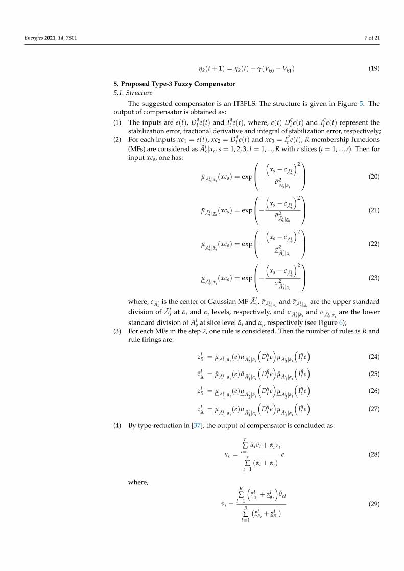
5. Proposed Type-3 Fuzzy Compensator5.1. Structure

The suggested compensator is an IT3FLS. The structure is given in Figure 5. Theoutput of compensator is obtained as:

(1) The inputs are e(t), Dqt e(t) and Iq

t e(t), where, e(t) Dqt e(t) and Iq

t e(t) represent thestabilization error, fractional derivative and integral of stabilization error, respectively;

(2) For each inputs xc1 = e(t), xc2 = Dqt e(t) and xc3 = Iq

t e(t), R membership functions(MFs) are considered as Al

s|αι, s = 1, 2, 3, l = 1, ..., R with r slices (ι = 1, ..., r). Then forinput xcs, one has:

µAls |αι

(xcs) = exp

−(

xs − cAls

)2

σ2Al

s |αι

(20)

µAls |αι

(xcs) = exp

−(

xs − cAls

)2

σ2Al

s |αι

(21)

µAl

s |αι(xcs) = exp

−(

xs − cAls

)2

σ2Al

s |αι

(22)

µAl

s |αι(xcs) = exp

−(

xs − cAls

)2

σ2Al

s |αι

(23)

where, cAls

is the center of Gaussian MF Als, σAl

s |αιand σAl

s |αιare the upper standard

division of Als at αι and αι levels, respectively, and σAl

s |αιand σAl

s |αιare the lower

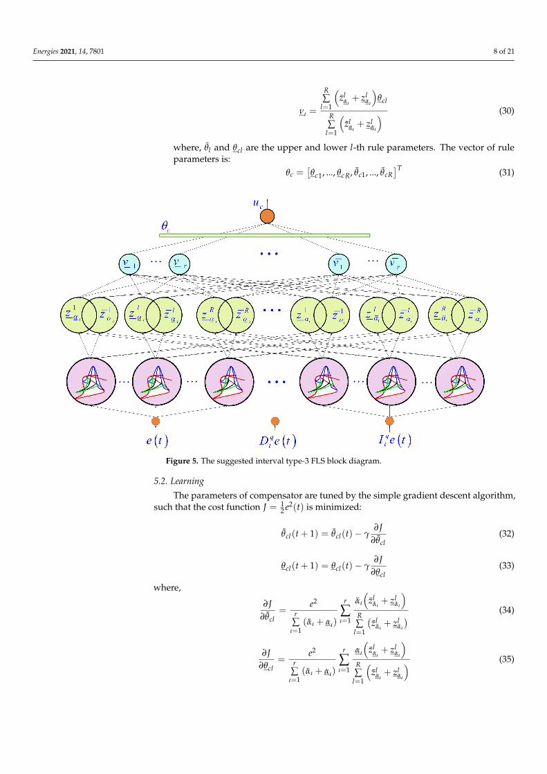
standard division of Als at slice level αι and αι, respectively (see Figure 6);

(3) For each MFs in the step 2, one rule is considered. Then the number of rules is R andrule firings are:

zlαι= µAl

1|αι(e)µAl

2|αι

(Dq

t e)

µAl3|αι

(Iqt e)

(24)

zlαι= µAl

1|αι(e)µAl

1|αι

(Dq

t e)

µAl1|αι

(Iqt e)

(25)

zlαι= µ

Al1|αι

(e)µAl

2|αι

(Dq

t e)

µAl

3|αι

(Iqt e)

(26)

zlαι= µ

Al1|αι

(e)µAl

1|αι

(Dq

t e)

µAl

1|αι

(Iqt e)

(27)

(4) By type-reduction in [37], the output of compensator is concluded as:

uc =

r∑

ι=1αινι + αινι

r∑

ι=1(αι + αι)

e (28)

where,

νι =

R∑

l=1

(zl

αι+ zl

αι

)θcl

R∑

l=1

(zl

αι+ zl

αι

) (29)

Energies 2021, 14, 7801 8 of 21

νι =

R∑

l=1

(zl

αι+ zl

αι

)θcl

R∑

l=1

(zl

αι+ zl

αι

) (30)

where, θl and θcl are the upper and lower l-th rule parameters. The vector of ruleparameters is:

θc =[θc1, ..., θcR, θc1, ..., θcR

]T (31)

Figure 5. The suggested interval type-3 FLS block diagram.

5.2. Learning

The parameters of compensator are tuned by the simple gradient descent algorithm,such that the cost function J = 1

2 e2(t) is minimized:

θcl(t + 1) = θcl(t)− γ∂J

∂θcl(32)

θcl(t + 1) = θcl(t)− γ∂J

∂θcl(33)

where,

∂J∂θcl

=e2

r∑

ι=1(αι + αι)

r

∑ι=1

αι

(zl

αι+ zl

αι

)R∑

l=1

(zl

αι+ zl

αι

) (34)

∂J∂θcl

=e2

r∑

ι=1(αι + αι)

r

∑ι=1

αι

(zl

αι+ zl

αι

)R∑

l=1

(zl

αι+ zl

αι

) (35)

Energies 2021, 14, 7801 9 of 21

01

1

100 -1

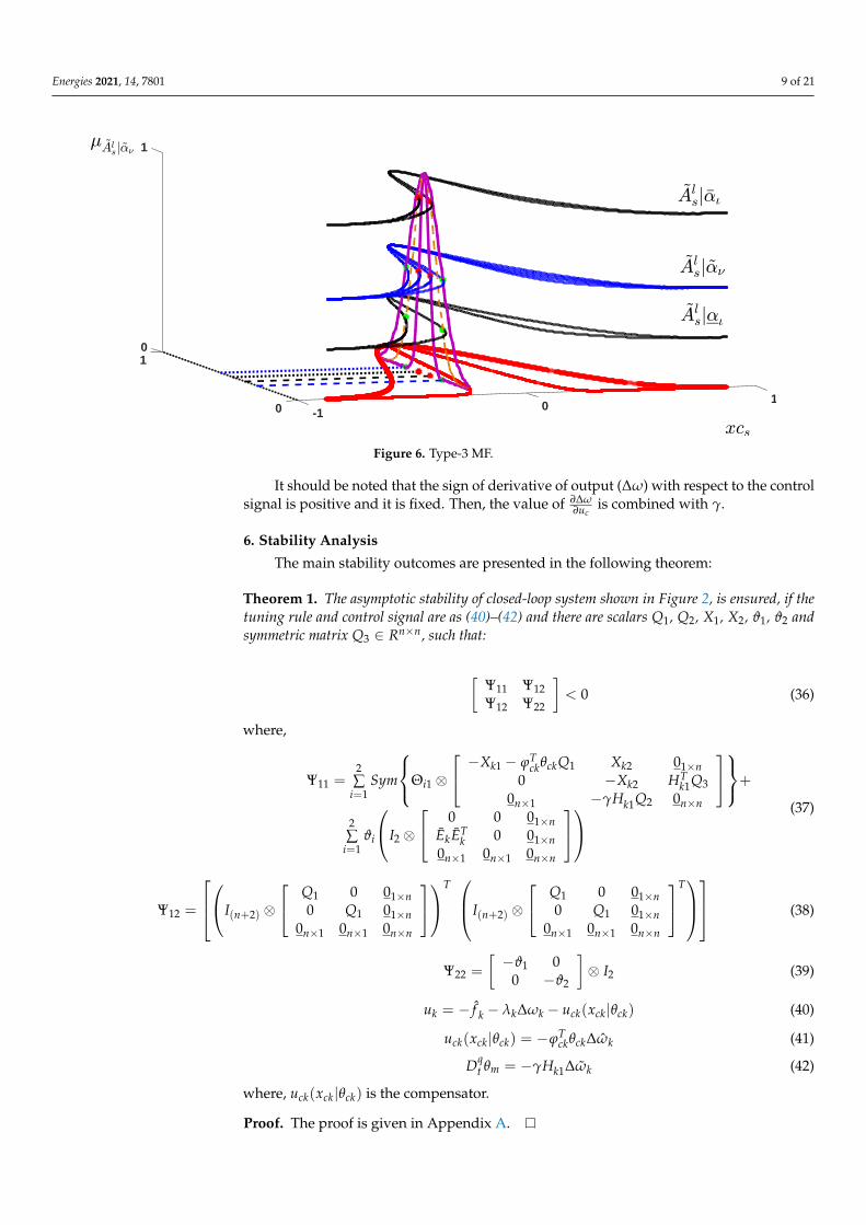
Figure 6. Type-3 MF.

It should be noted that the sign of derivative of output (∆ω) with respect to the controlsignal is positive and it is fixed. Then, the value of ∂∆ω

∂ucis combined with γ.

6. Stability Analysis

The main stability outcomes are presented in the following theorem:

Theorem 1. The asymptotic stability of closed-loop system shown in Figure 2, is ensured, if thetuning rule and control signal are as (40)–(42) and there are scalars Q1, Q2, X1, X2, ϑ1, ϑ2 andsymmetric matrix Q3 ∈ Rn×n, such that:

[Ψ11 Ψ12Ψ12 Ψ22

]< 0 (36)

where,

Ψ11 =2∑

i=1Sym

Θi1 ⊗

−Xk1 − ϕTckθckQ1 Xk2 01×n

0 −Xk2 HTk1Q3

0n×1 −γHk1Q2 0n×n

+

2∑

i=1ϑi

I2 ⊗

0 0 01×nEkET

k 0 01×n0n×1 0n×1 0n×n

(37)

Ψ12 =

I(n+2) ⊗

Q1 0 01×n0 Q1 01×n

0n×1 0n×1 0n×n

T I(n+2) ⊗

Q1 0 01×n0 Q1 01×n

0n×1 0n×1 0n×n

T (38)

Ψ22 =

[−ϑ1 0

0 −ϑ2

]⊗ I2 (39)

uk = − f k − λk∆ωk − uck(xck|θck) (40)

uck(xck|θck) = −ϕTckθck∆ωk (41)

Dqt θm = −γHk1∆ωk (42)

where, uck(xck|θck) is the compensator.

Proof. The proof is given in Appendix A.

Energies 2021, 14, 7801 10 of 21

7. Simulation

The regulation outcomes of the designed LFC is examined in several scenarios, suchas time-varying dynamics, suddenly changes in mechanical power, time-varying solarradiation, multiple load perturbation, and so on.

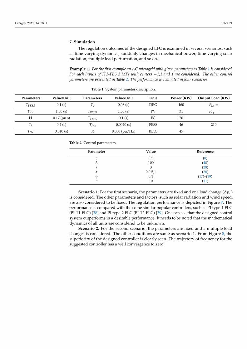
Example 1. For the first example an AC microgrid with given parameters as Table 1 is considered.For each inputs of IT3-FLS 3 MFs with centers −1,1 and 1 are considered. The other controlparameters are presented in Table 2. The performance is evaluated in four scenarios.

Table 1. System parameter description.

Parameters Value/Unit Parameters Value/Unit Unit Power (KW) Output Load (KW)

TBESS 0.1 (s) Tg 0.08 (s) DEG 160 PL2 =

TPV 1.80 (s) TWTG 1.50 (s) PV 31 PL1 =

H 0.17 (pu s) TFESS 0.1 (s) FC 70

Tt 0.4 (s) TI/c 0.0040 (s) FESS 46 210

TIN 0.040 (s) R 0.330 (pu/Hz) BESS 45

Table 2. Control parameters.

Parameter Value Reference

q 0.5 (8)λ 100 (40)r 3 (28)α 0,0.5,1 (28)γ 0.1 (17)–(19)n 10 (11)

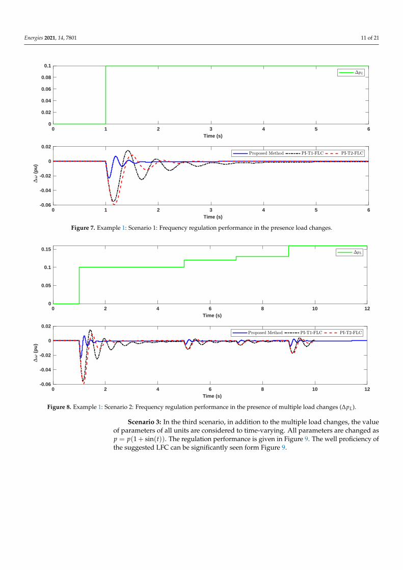
Scenario 1: For the first scenario, the parameters are fixed and one load change (∆pL)is considered. The other parameters and factors, such as solar radiation and wind speed,are also considered to be fixed. The regulation performance is depicted in Figure 7. Theperformance is compared with the some similar popular controllers, such as PI type-1 FLC(PI-T1-FLC) [38] and PI type-2 FLC (PI-T2-FLC) [39]. One can see that the designed controlsystem outperforms in a desirable performance. It needs to be noted that the mathematicaldynamics of all units are considered to be unknown.

Scenario 2: For the second scenario, the parameters are fixed and a multiple loadchanges is considered. The other conditions are same as scenario 1. From Figure 8, thesuperiority of the designed controller is clearly seen. The trajectory of frequency for thesuggested controller has a well convergence to zero.

Energies 2021, 14, 7801 11 of 21

0 1 2 3 4 5 6 Time (s)

0

0.02

0.04

0.06

0.08

0.1

0 1 2 3 4 5 6 Time (s)

-0.06

-0.04

-0.02

0

0.02

(

pu

)

Figure 7. Example 1: Scenario 1: Frequency regulation performance in the presence load changes.

0 2 4 6 8 10 12 Time (s)

0

0.05

0.1

0.15

0 2 4 6 8 10 12 Time (s)

-0.06

-0.04

-0.02

0

0.02

(

pu

)

Figure 8. Example 1: Scenario 2: Frequency regulation performance in the presence of multiple load changes (∆pL).

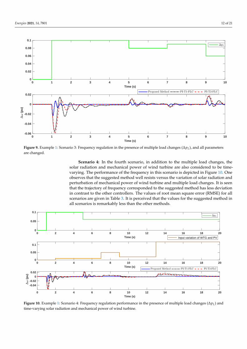
Scenario 3: In the third scenario, in addition to the multiple load changes, the valueof parameters of all units are considered to time-varying. All parameters are changed asp = p(1 + sin(t)). The regulation performance is given in Figure 9. The well proficiency ofthe suggested LFC can be significantly seen form Figure 9.

Energies 2021, 14, 7801 12 of 21

0 1 2 3 4 5 6 7 8 9 10 Time (s)

0

0.02

0.04

0.06

0.08

0.1

0 1 2 3 4 5 6 7 8 9 10 Time (s)

-0.06

-0.04

-0.02

0

0.02

(

pu

)

Figure 9. Example 1: Scenario 3: Frequency regulation in the presence of multiple load changes (∆pL), and all parametersare changed.

Scenario 4: In the fourth scenario, in addition to the multiple load changes, thesolar radiation and mechanical power of wind turbine are also considered to be time-varying. The performance of the frequency in this scenario is depicted in Figure 10. Oneobserves that the suggested method well resists versus the variation of solar radiation andperturbation of mechanical power of wind turbine and multiple load changes. It is seenthat the trajectory of frequency corresponded to the suggested method has less deviationin contrast to the other controllers. The values of root mean square error (RMSE) for allscenarios are given in Table 3. It is perceived that the values for the suggested method inall scenarios is remarkably less than the other methods.

0 2 4 6 8 10 12 14 16 18 20 Time (s)

0

0.05

0.1

0 2 4 6 8 10 12 14 16 18 20 Time (s)

0

0.05

0.1

Input variation of WTG and PV

0 2 4 6 8 10 12 14 16 18 20 Time (s)

-0.04

-0.02

0

0.02

(

pu

)

Figure 10. Example 1: Scenario 4: Frequency regulation performance in the presence of multiple load changes (∆pL) andtime-varying solar radiation and mechanical power of wind turbine.

Energies 2021, 14, 7801 13 of 21

Table 3. Regulation comparison by various controllers.

RMSE RMSE

Scenario Proposed Method PI-T1-FLC PI-T2-FLC

1 0.0027 0.0105 0.01072 0.0022 0.0084 0.00853 0.0017 0.0064 0.00664 0.0018 0.0078 0.0075

Example 2. For the second example, the IEEE 39-bus test system is taken to account. Thedemand response for the first, second, and third area are considered as 98.77, 22.21, and 54.6 MW,respectively. The power capacity of all units are given in Table 4. The other conditions are sameas [40]. The performance is examined in three scenarios.

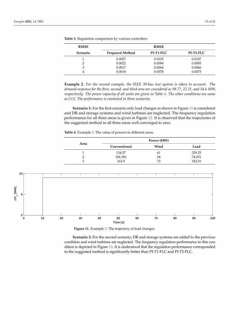
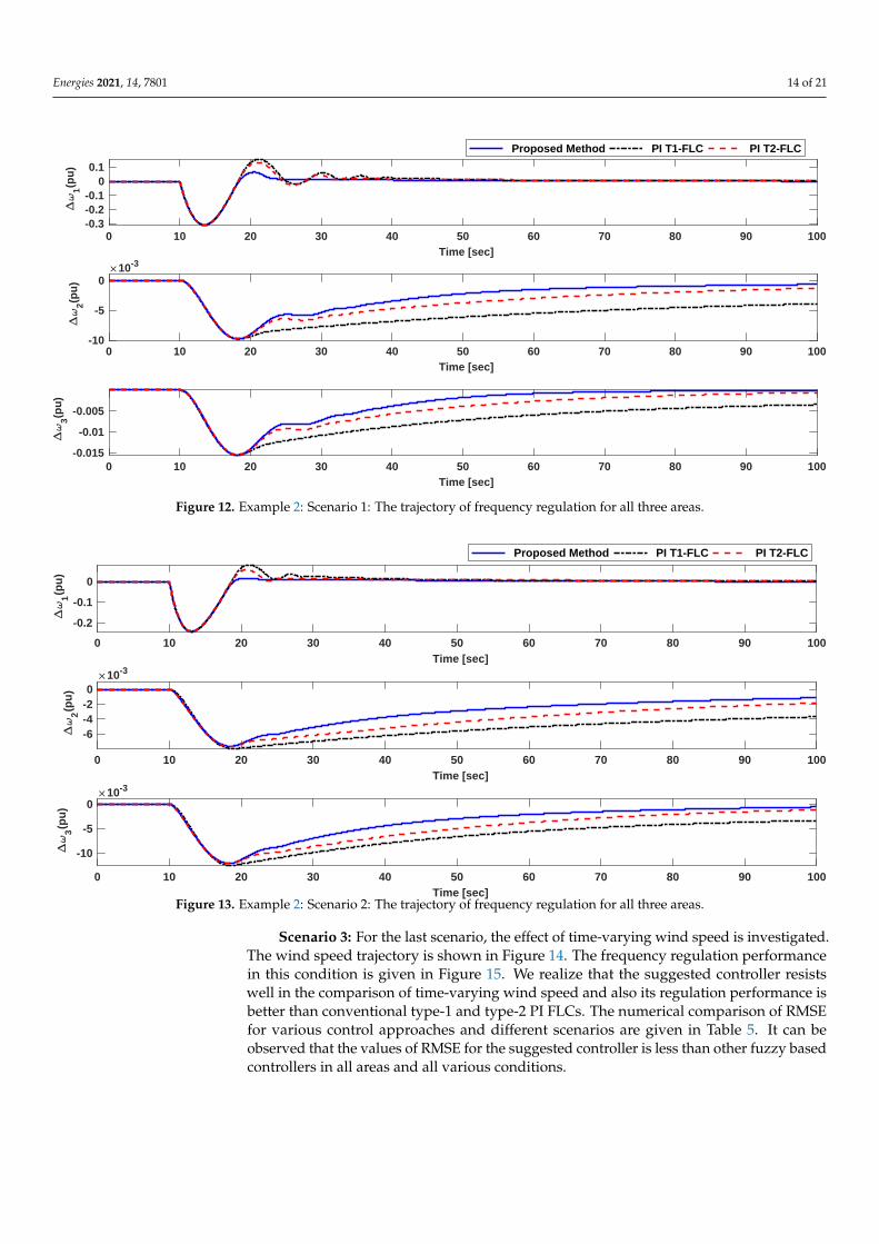
Scenario 1: For the first scenario only load changes as shown in Figure 11 is consideredand DR and storage systems and wind turbines are neglected. The frequency regulationperformance for all three areas is given in Figure 12. It is observed that the trajectories ofthe suggested method in all three areas well converged to zero.

Table 4. Example 2: The value of powers in different areas.

AreaPower (MW)

Conventional Wind Load

1 134.57 61 329.252 106.381 54 74.0513 163.9 72 182.01

0 10 20 30 40 50 60 70 80 90 100 Time [s]

0

5

10

P

L [

MW

]

Figure 11. Example 2: The trajectory of load changes.

Scenario 2: For the second scenario, DR and storage systems are added to the previouscondition and wind turbines are neglected. The frequency regulation performance in this con-dition is depicted in Figure 13. It is understood that the regulation performance correspondedto the suggested method is significantly better than PI-T1-FLC and PI-T2-FLC.

Energies 2021, 14, 7801 14 of 21

0 10 20 30 40 50 60 70 80 90 100 Time [sec]

-0.3-0.2-0.1

00.1

1(p

u)

Proposed Method PI T1-FLC PI T2-FLC

0 10 20 30 40 50 60 70 80 90 100 Time [sec]

-10

-5

0

2(p

u)

10-3

0 10 20 30 40 50 60 70 80 90 100 Time [sec]

-0.015

-0.01

-0.005

3(p

u)

Figure 12. Example 2: Scenario 1: The trajectory of frequency regulation for all three areas.

0 10 20 30 40 50 60 70 80 90 100 Time [sec]

-0.2

-0.1

0

1(p

u)

Proposed Method PI T1-FLC PI T2-FLC

0 10 20 30 40 50 60 70 80 90 100 Time [sec]

-6-4-20

2(p

u)

10-3

0 10 20 30 40 50 60 70 80 90 100 Time [sec]

-10

-5

0

3(p

u)

10-3

Figure 13. Example 2: Scenario 2: The trajectory of frequency regulation for all three areas.

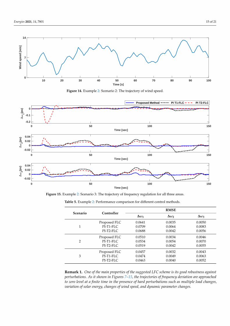
Scenario 3: For the last scenario, the effect of time-varying wind speed is investigated.The wind speed trajectory is shown in Figure 14. The frequency regulation performancein this condition is given in Figure 15. We realize that the suggested controller resistswell in the comparison of time-varying wind speed and also its regulation performance isbetter than conventional type-1 and type-2 PI FLCs. The numerical comparison of RMSEfor various control approaches and different scenarios are given in Table 5. It can beobserved that the values of RMSE for the suggested controller is less than other fuzzy basedcontrollers in all areas and all various conditions.

Energies 2021, 14, 7801 15 of 21

10 20 30 40 50 60 70 80 90 100 Time [s]

0

7

14

Win

d s

pee

d [

m/s

]

Figure 14. Example 2: Scenario 2: The trajectory of wind speed.

0 50 100 150 Time [sec]

-0.2

-0.1

0

1(p

u)

Proposed Method PI T1-FLC PI T2-FLC

0 50 100 150 Time [sec]

-0.02

0

0.02

0.04

2(p

u)

0 50 100 150 Time [sec]

-0.02

0

0.02

0.04

3(p

u)

Figure 15. Example 2: Scenario 3: The trajectory of frequency regulation for all three areas.

Table 5. Example 2: Performance comparison for different control methods.

Scenario ControllerRMSE

∆ω1 ∆ω2 ∆ω3

1Proposed FLC 0.0641 0.0035 0.0050

PI-T1-FLC 0.0709 0.0064 0.0083PI-T2-FLC 0.0688 0.0042 0.0056

2Proposed FLC 0.0510 0.0034 0.0046

PI-T1-FLC 0.0534 0.0054 0.0070PI-T2-FLC 0.0519 0.0042 0.0055

3Proposed FLC 0.0457 0.0032 0.0043

PI-T1-FLC 0.0474 0.0049 0.0063PI-T2-FLC 0.0463 0.0040 0.0052

Remark 1. One of the main properties of the suggested LFC scheme is its good robustness againstperturbations. As it shown in Figures 7–15, the trajectories of frequency deviation are approachedto zero level at a finite time in the presence of hard perturbations such as multiple load changes,variation of solar energy, changes of wind speed, and dynamic parameter changes.

Energies 2021, 14, 7801 16 of 21

8. Conclusions

In this study, a new adaptive FLC is designed for frequency regulation in multi-areapower systems. The suggested controller is constructed by an error feedback controller,dynamic estimated model, and IT3-FLS. The gains of error feedback controller and thetuning rules of the dynamic model is extracted through the LMI stability analysis. Theunknown dynamics of the units are estimated online by the suggested dynamic fractional-order RBM and deep learning CD algorithm. The effectiveness of the schemed controlapproach is examined various conditions. For the first simulation example, an ac mi-crogrid including loads, PVs, micro-turbines, WT, FESS, and BESS is considered and theperformance is evaluated in four scenarios. For the first scenario, only small changes inthe load is considered. In the second, multiple load changes is considered. For the thirdone, the issue of time-varying factors in all units is also added to the previous conditionand finally in the fourth scenario the effect variation of irradiation and wind speed isexamined. For the second simulation, the schemed controller is applied on the practicalIEEE 39-bus system. Similar to the example one, the performance is evaluated in variousconditions and effect of time-varying wind speed, multiple load changes, and DR andstorage systems are investigated. In all cases the performance is compared with the someother popular controllers, such as PI-T1-FLC and PI-T2-FLC. One observes that suggestedcontrol system results in desirable frequency regulation performance in versus of variouspractical conditions and has clear superiority in contrast to the conventional FLCs.

Author Contributions: Conceptualization, A.M., O.C., A.A.A., B.F.F. and A.B.; Data curation, A.M.,O.C., A.A.A., B.F.F. and A.B.; Formal analysis, A.M., O.C., A.A.A., B.F.F. and A.B.; Funding acquisition,A.A.A. and B.F.F.; Investigation, A.M., O.C., A.A.A., B.F.F. and A.B.; Methodology, A.M., O.C., A.A.A.,B.F.F. and A.B.; Software, A.M., O.C., A.A.A., B.F.F. and A.B.; Supervision, A.M., O.C., A.A.A., B.F.F.and A.B.; Visualization, A.M., O.C., A.A.A., B.F.F. and A.B.; Writing—original draft, A.M., O.C.,A.A.A., B.F.F. and A.B. All authors have read and agreed to the published version of the manuscript.

Funding: Taif University Researchers Supporting Project number (TURSP-2020/260), Taif University,Taif, Saudi Arabia.

Institutional Review Board Statement: Not applicable.

Informed Consent Statement: Not applicable.

Data Availability Statement: The study do not report any data.

Acknowledgments: The authors would like to express their sincere thanks to Rabia Safdar for hishelp in improving this paper.

Conflicts of Interest: The authors declare no conflict of interest.

Appendix A. Stability Analysis

The following Lemmas are applied to prove results of Theorem 1.

Lemma A1 ([41]). The following equations are equivalent for a real matrix Π = ΠT :

(a) Π =

[Π11 Π12∗ Π22

]> 0

(b) Π11 > 0, and Π22 −ΠT12Π−1

11 Π12 > 0(c) Π22 > 0, and Π11 −ΠT

12Π−122 Π12 > 0

Lemma A2 ([42]). Consider real matrices U and L and the following relation:

UF(t)L + LT FT(t)UT < 0

Energies 2021, 14, 7801 17 of 21

if FT(t)F(t) ≤ I, then there exists a ϑ, such that

ϑUUT + ϑ−1LT L < 0

Lemma A3 ([43]). The asymptotic stability of system Dqt x(t) = Ax(t) is authenticated if there

exist two symmetric matrices Πj1 ∈ <n×n, j = 1, 2 with positive definite property and twoskew-symmetric matrices Πj2 ∈ <n×n, j = 1, 2, such that:

2∑

i=1

2∑

j=1Sym

Θij ⊗

(AΠij

)< 0,[

Π11 Π12−Π12 Π11

]> 0,

[Π21 Π22−Π22 Π21

]> 0

(A1)

where

Θ11 =

[sin πq

2 − cos πq2

cos πq2 sin πq

2

], Θ12 =

[cos πq

2 sin πq2

− sin πq2 cos πq

2

]Θ21 =

[sin πq

2 cos πq2

− cos πq2 sin πq

2

], Θ22 =

[− cos πq

2 sin πq2

− sin πq2 − cos πq

2

]SymX = X + XT and ⊗ is Kronecker product.

From the universal approximation feature of neural networks and by considering theoptimal MLP the dynamics of ∆ωk can be written as:

Dqt ∆ωk = f ∗k (xk|θ∗km, ξk, εk, ηk) + Ek + uk (A2)

where, θ∗km is the vector of optimal parameters and Ek is the approximation error. From (8)and (A2), the dynamic of estimation error ∆ωk is obtained as:

Dqt ∆ωk = f ∗k (xk|θ∗m, ξk, εk, ηk)− f k(xk|θm, ξk, εk, ηk)− χk∆ωk + Ek (A3)

where, ∆ωk = ∆ωk − ∆ωk. Consider the flowing definitions:

θm = θ∗m − θmf ∗k (xk|θ∗m, ξk, εk, ηk)− f k(xk|θm, ξk, εk, ηk) = θT

mHk1(A4)

From (A4), Dqt ∆ωk in (A3) is rewritten as:

Dqt ∆ωk = θT

mHk1 − χk∆ωk + Ek (A5)

The approximation error Ek can be written as:

Ek = Dkφk(t)∆ωk (A6)

where, Ek is the upper bound of Ek and 0 ≤ φk(t) ≤ 1. From (A6), the Equation (A5) isrewritten as:

Dqt ∆ωk = θT

mHk1 − χk∆ωk + Ekφk(t)∆ωk (A7)

By applying the control signal (40), the dynamic of ∆ωk becomes:

Dqt ∆ωk = −λk∆ωk + χk∆ωk − uck(xck|θck) (A8)

By substituting uck(xck|θck) from (41), one has:

Dqt ∆ωk = −λk∆ωk + χk∆ωk − ϕT

ckθck∆ωk (A9)

Energies 2021, 14, 7801 18 of 21

In the vector form, one has:

Dqt

∆ωk∆ωkθm

=

−λk χk 01×n0 −χk HT

k10n×1 −γHk1 0n×n

∆ωk∆ωkθm

+

−uck(xck|θc)Ek0

(A10)

where, n is number of elements in Hk1.Considering (Lemma A3) and by choosing P12 = P22 = 0 and

P11 = P21 =

Q1 0 01×n0 Q2 01×n

0n×1 0n×1 Q3

(A11)

It is derived that system (A10) is asymptotically stable if:

2

∑i=1

Sym

Θi1 ⊗

−λk − ϕTckθck χk 01×n

Ekφk(t) −χk HTk1

0n×1 −γHk1 0n×n

Q1 0 01×n0 Q2 01×n

0n×1 0n×1 Q3

< 0 (A12)

The inequality (A12) can be rewritten as:

2∑

i=1Sym

Θi1 ⊗

−λkQ1 − ϕTckθckQ1 χkQ2 01×n

0 −χkQ2 HTk1Q3

0n×1 −γHk1Q2 0n×n

+

2∑

i=1Sym

Θi1 ⊗

0 0 01×nEkφk(t)Q1 0 01×n

0n×1 0n×1 0n×n

< 0

(A13)

From (A13), one has:

2∑

i=1Sym

Θi1 ⊗

0 0 01×nEkφk(t)Q1 0 01×n

0n×1 0n×1 0n×n

=

2∑

i=1Sym

Θi1 ⊗

0 0 01×nEk 0 01×n

0n×1 0n×1 0n×n

φk(t) 0 01×n0 φk(t) 01×n

0n×1 0n×1 0n×n

Q1 0 01×n0 Q1 01×n

0n×1 0n×1 0n×n

(A14)

From Equation (A14), the second term is rewritten as:

2∑

i=1Sym

Θi1 ⊗

0 0 01×nEk 0 01×n

0n×1 0n×1 0n×n

φk(t) 0 01×n0 φk(t) 01×n

0n×1 0n×1 0n×n

Q1 0 01×n0 Q1 01×n

0n×1 0n×1 0n×n

=

2∑

i=1Sym

Θi1 ⊗

0 0 01×nEk 0 01×n

0n×1 0n×1 0n×n

.I(n+2) ⊗

φk(t) 0 01×n0 φk(t) 01×n

0n×1 0n×1 0n×n

.I(n+2) ⊗

Q1 0 01×n0 Q1 01×n

0n×1 0n×1 0n×n

(A15)

Energies 2021, 14, 7801 19 of 21

From (A15), it can be written:I(n+2) ⊗

φk(t) 0 01×n0 φk(t) 01×n

0n×1 0n×1 0n×n

I(n+2) ⊗

φk(t) 0 01×n0 φk(t) 01×n

0n×1 0n×1 0n×n

T

=I(n+2) ⊗

φk(t)φTk (t) 0 01×n

0 φk(t)φTk (t) 01×n

0n×1 0n×1 0n×n

≤ I(n+2)

(A16)

Then form (A16) and Lemma A2, the equation (A14) is rewritten as:

2∑

i=1Sym

Θi1 ⊗

0 0 01×nEkφk(t)Q1 0 01×n

0n×1 0n×1 0n×n

≤2∑

i=1ϑi

Θi1 ⊗

0 0 01×nEk 0 01×n

0n×1 0n×1 0n×n

.

Θi1 ⊗

0 0 01×nEk 0 01×n

0n×1 0n×1 0n×n

T

+ϑ−1i

I(n+2) ⊗

Q1 0 01×n0 Q1 01×n

0n×1 0n×1 0n×n

T

.

I(n+2) ⊗

Q1 0 01×n0 Q1 01×n

0n×1 0n×1 0n×n

(A17)

From (A17), the inequality (A13) becomes:

2∑

i=1Sym

Θi1 ⊗

−λkQ1 − ϕTckθckQ1 χkQ2 01×n

0 −χkQ2 HTk1Q3

0n×1 −γHk1Q2 0n×n

+

2∑

i=1ϑi

Θi1 ⊗

0 0 01×nEk 0 01×n

0n×1 0n×1 0n×n

.

Θi1 ⊗

0 0 01×nEk 0 01×n

0n×1 0n×1 0n×n

T

+ϑ−1i

I(n+2) ⊗

Q1 0 01×n0 Q1 01×n

0n×1 0n×1 0n×n

T

.

I(n+2) ⊗

Q1 0 01×n0 Q1 01×n

0n×1 0n×1 0n×n

< 0

(A18)

By considering Xk1 = λkQ1, Xk2 = χkQ2 and ΘTi1Θi1 = I2, the inequality (A18), becomes:

2∑

i=1Sym

Θi1 ⊗

−Xk1 − ϕTckθckQ1 Xk2 01×n

0 −Xk2 HTk1Q3

0n×1 −γHk1Q2 0n×n

+

2∑

i=1ϑi

I2 ⊗

0 0 01×nEkET

k 0 01×n0n×1 0n×1 0n×n

+ϑ−1

i

I(n+2) ⊗

Q1 0 01×n0 Q1 01×n

0n×1 0n×1 0n×n

T

.

I(n+2) ⊗

Q1 0 01×n0 Q1 01×n

0n×1 0n×1 0n×n

< 0

(A19)

From (A19), one can has:

2∑

i=1ϑ−1

i

I(n+2) ⊗

Q1 0 01×n0 Q1 01×n

0n×1 0n×1 0n×n

T

.

I(n+2) ⊗

Q1 0 01×n0 Q1 01×n

0n×1 0n×1 0n×n

=

I(n+2) ⊗

Q1 0 01×n0 Q1 01×n

0n×1 0n×1 0n×n

T

ϑ−11

I(n+2) ⊗

Q1 0 01×n0 Q1 01×n

0n×1 0n×1 0n×n

+

Energies 2021, 14, 7801 20 of 21

I(n+2) ⊗

Q1 0 01×n0 Q1 01×n

0n×1 0n×1 0n×n

T

ϑ−12

I(n+2) ⊗

Q1 0 01×n0 Q1 01×n

0n×1 0n×1 0n×n

=

I(n+2) ⊗

Q1 0 01×n0 Q1 01×n

0n×1 0n×1 0n×n

T I(n+2) ⊗

Q1 0 01×n0 Q1 01×n

0n×1 0n×1 0n×n

T

T

.

([ϑ1 00 ϑ2

]⊗ I2

)−1

.I(n+2) ⊗

Q1 0 01×n0 Q1 01×n

0n×1 0n×1 0n×n

T I(n+2) ⊗

Q1 0 01×n0 Q1 01×n

0n×1 0n×1 0n×n

T (A20)

From Equations (A19) and (A20) and Lemma A1, the inequality (36) is obtained. Thiscompletes the proof.

References1. Mihet-Popa, L.; Saponara, S. Power Converters, Electric Drives and Energy Storage Systems for Electrified Transportation and

Smart Grid Applications. Energies 2021, 14, 4142. [CrossRef]2. Subramanian, S.; Sankaralingam, C.; Elavarasan, R.M.; Vijayaraghavan, R.R.; Raju, K.; Mihet-Popa, L. An Evaluation on Wind

Energy Potential Using Multi-Objective Optimization Based Non-Dominated Sorting Genetic Algorithm III. Sustainability 2021,13, 410. [CrossRef]

3. Armghan, A.; Azeem, M.K.; Armghan, H.; Yang, M.; Alenezi, F.; Hassan, M. Dynamical Operation Based Robust NonlinearControl of DC Microgrid Considering Renewable Energy Integration. Energies 2021, 14, 3988. [CrossRef]

4. Marti-Puig, P.; Blanco-M, A.; Cárdenas, J.J.; Cusidó, J.; Solé-Casals, J. Feature selection algorithms for wind turbine failureprediction. Energies 2019, 12, 453. [CrossRef]

5. Armghan, A.; Hassan, M.; Armghan, H.; Yang, M.; Alenezi, F.; Azeem, M.K.; Ali, N. Barrier Function Based Adaptive SlidingMode Controller for a Hybrid AC/DC Microgrid Involving Multiple Renewables. Appl. Sci. 2021, 11, 8672. [CrossRef]

6. Shabani, H.; Vahidi, B.; Ebrahimpour, M. A robust PID controller based on imperialist competitive algorithm for load-frequencycontrol of power systems. ISA Trans. 2013, 52, 88–95. [CrossRef]

7. Farahani, M.; Ganjefar, S.; Alizadeh, M. PID controller adjustment using chaotic optimisation algorithm for multi-area loadfrequency control. IET Control Theory Appl. 2012, 6, 1984–1992. [CrossRef]

8. Wies, R.W.; Chukkapalli, E.; Mueller-Stoffels, M. Improved frequency regulation in mini-grids with high wind contribution usingonline genetic algorithm for PID tuning. In Proceedings of the 2014 IEEE PES General Meeting|Conference & Exposition, IEEE,New York, NY, USA, 27–31 July 2014; pp. 1–5.

9. Sahoo, B.; Panda, S. Improved grey wolf optimization technique for fuzzy aided PID controller design for power system frequencycontrol. Sustain. Energy Grids Netw. 2018, 16, 278–299. [CrossRef]

10. Abedinia, O.; Naderi, M.S.; Ghasemi, A. Robust LFC in deregulated environment: Fuzzy PID using HBMO. In Proceedings ofthe 2011 10th International Conference on Environment and Electrical Engineering, IEEE, New York, NY, USA, 8–11 May 2011;pp. 1–4.

11. Ali, E.; Abd-Elazim, S. BFOA based design of PID controller for two area load frequency control with nonlinearities. Int. J. Electr.Power Energy Syst. 2013, 51, 224–231. [CrossRef]

12. Kouba, N.E.Y.; Menaa, M.; Hasni, M.; Boudour, M. LFC enhancement concerning large wind power integration using newoptimised PID controller and RFBs. IET Gener. Transm. Distrib. 2016, 10, 4065–4077. [CrossRef]

13. Kontogiannis, D.; Bargiotas, D.; Daskalopulu, A. Fuzzy control system for smart energy management in residential buildingsbased on environmental data. Energies 2021, 14, 752. [CrossRef]

14. Kontogiannis, D.; Bargiotas, D.; Daskalopulu, A. Minutely active power forecasting models using neural networks. Sustainability2020, 12, 3177. [CrossRef]

15. Cusidó, J.; López, A.; Beretta, M. Fault-Tolerant Control of a Wind Turbine Generator Based on Fuzzy Logic and Using EnsembleLearning. Energies 2021, 14, 5167. [CrossRef]

16. Yesil, E. Interval type-2 fuzzy PID load frequency controller using Big Bang–Big Crunch optimization. Appl. Soft Comput. 2014,15, 100–112. [CrossRef]

17. Khooban, M.H.; Niknam, T. A new intelligent online fuzzy tuning approach for multi-area load frequency control: Self AdaptiveModified Bat Algorithm. Int. J. Electr. Power Energy Syst. 2015, 71, 254–261. [CrossRef]

18. Sahu, B.K.; Pati, S.; Mohanty, P.K.; Panda, S. Teaching–learning based optimization algorithm based fuzzy-PID controller forautomatic generation control of multi-area power system. Appl. Soft Comput. 2015, 27, 240–249. [CrossRef]

Energies 2021, 14, 7801 21 of 21

19. Gheisarnejad, M. An effective hybrid harmony search and cuckoo optimization algorithm based fuzzy PID controller for loadfrequency control. Appl. Soft Comput. 2018, 65, 121–138. [CrossRef]

20. Kouba, N.E.Y.; Menaa, M.; Hasni, M.; Boudour, M. Application of multi-verse optimiser-based fuzzy-PID controller to improvepower system frequency regulation in presence of HVDC link. Int. J. Intell. Eng. Inform. 2018, 6, 182–203. [CrossRef]

21. Chintu, J.M.R.; Sahu, R.K. Differential Evolution Optimized Fuzzy PID Controller for Automatic Generation Control ofInterconnected Power System. In Computational Intelligence in Pattern Recognition; Springer: Berlin/Heidelberg, Germany, 2020;pp. 123–132.

22. Arya, Y. AGC of two-area electric power systems using optimized fuzzy PID with filter plus double integral controller. J. Frankl.Inst. 2018, 355, 4583–4617. [CrossRef]

23. Jena, T.; Debnath, M.K.; Sanyal, S.K. Optimal fuzzy-PID controller with derivative filter for load frequency control includingUPFC and SMES. Int. J. Electr. Comput. Eng. 2019, 9, 2813. [CrossRef]

24. Debnath, M.K.; Jena, T.; Sanyal, S.K. Frequency control analysis with PID-fuzzy-PID hybrid controller tuned by modified GWOtechnique. Int. Trans. Electr. Energy Syst. 2019, 29, e12074. [CrossRef]

25. Khamari, D.; Sahu, R.K.; Panda, S. A Modified Moth Swarm Algorithm-Based Hybrid Fuzzy PD–PI Controller for FrequencyRegulation of Distributed Power Generation System with Electric Vehicle. J. Control Autom. Electr. Syst. 2020, 31, 1–18. [CrossRef]

26. Alam, M.S.; Al-Ismail, F.S.; Abido, M.A. PV/Wind-Integrated Low-Inertia System Frequency Control: PSO-Optimized Fractional-Order PI-Based SMES Approach. Sustainability 2021, 13, 7622. [CrossRef]

27. Alam, M.S.; Al-Ismail, F.S.; Abido, M.A. Power management and state of charge restoration of direct current microgrid withimproved voltage-shifting controller. J. Energy Storage 2021, 44, 103253. [CrossRef]

28. Jena, N.K.; Sahoo, S.; Nanda, A.B.; Sahu, B.K.; Mohanty, K.B. Frequency Regulation in an Islanded Microgrid with OptimalFractional Order PID Controller. In Advances in Intelligent Computing and Communication; Springer: Berlin/Heidelberg, Germany,2020; pp. 447–457.

29. Singh, A.; Suhag, S. Frequency regulation in an AC microgrid interconnected with thermal system employing multiverse-optimised fractional order-PID controller. Int. J. Sustain. Energy 2020, 39, 250–262. [CrossRef]

30. Satapathy, P.; Debnath, M.K.; Mohanty, P.K.; Sahu, B.K. Participation of Geothermal and Dish-Stirling Solar Power Plant for LFCAnalysis Using Fractional-Order Controller. In Innovation in Electrical Power Engineering, Communication, and Computing Technology;Springer: Berlin/Heidelberg, Germany, 2020; pp. 113–122.

31. Saxena, S. Load frequency control strategy via fractional-order controller and reduced-order modeling. Int. J. Electr. Power EnergySyst. 2019, 104, 603–614. [CrossRef]

32. Babaei, F.; Lashkari, Z.B.; Safari, A.; Farrokhifar, M.; Salehi, J. Salp swarm algorithm-based fractional-order PID controller forLFC systems in the presence of delayed EV aggregators. IET Electr. Syst. Transp. 2020. [CrossRef]

33. Lamba, R.; Singla, S.K.; Sondhi, S. Design of Fractional Order PID Controller for Load Frequency Control in Perturbed Two AreaInterconnected System. Electr. Power Components Syst. 2019, 47, 998–1011. [CrossRef]

34. Tian, E.; Peng, C. Memory-Based Event-Triggering H∞ Load Frequency Control for Power Systems Under Deception Attacks.IEEE Trans. Cybern. 2020. [CrossRef]

35. Kanagaraj, N. Photovoltaic and Thermoelectric Generator Combined Hybrid Energy System with an Enhanced Maximum PowerPoint Tracking Technique for Higher Energy Conversion Efficiency. Sustainability 2021, 13, 3144.

36. Kanagaraj, N.; Rezk, H. Dynamic Voltage Restorer Integrated with Photovoltaic-Thermoelectric Generator for Voltage Distur-bances Compensation and Energy Saving in Three-Phase System. Sustainability 2021, 13, 3511. [CrossRef]

37. Mohammadzadeh, A.; Sabzalian, M.H.; Zhang, W. An interval type-3 fuzzy system and a new online fractional-order learningalgorithm: Theory and practice. IEEE Trans. Fuzzy Syst. 2019. [CrossRef]

38. Arya, Y.; Kumar, N. Design and analysis of BFOA-optimized fuzzy PI/PID controller for AGC of multi-area tradi-tional/restructured electrical power systems. Soft Comput. 2017, 21, 6435–6452. [CrossRef]

39. Meziane, K.B.; Naoual, R.; Boumhidi, I. Type-2 Fuzzy Logic based on PID controller for AGC of Two-Area with Three SourcePower System including Advanced TCSC. Procedia Comput. Sci. 2019, 148, 455–464. [CrossRef]

40. Babahajiani, P.; Shafiee, Q.; Bevrani, H. Intelligent demand response contribution in frequency control of multi-area powersystems. IEEE Trans. Smart Grid 2016, 9, 1282–1291. [CrossRef]

41. Boyd, S.P.; El Ghaoui, L.; Feron, E.; Balakrishnan, V. Linear Matrix Inequalities in System and Control Theory; SIAM: Philadelphia,PA, USA, 1994; Volume 15.

42. Xie, L. Output feedback H-infinity control of systems with parameter uncertainty. Int. J. Control 1996, 63, 741–750. [CrossRef]43. Lu, J.G.; Chen, Y.Q. Robust stability and stabilization of fractional-order interval systems with the fractional order α: The

0 ≤ α ≤ 1 case. Autom. Control IEEE Trans. 2010, 55, 152–158.