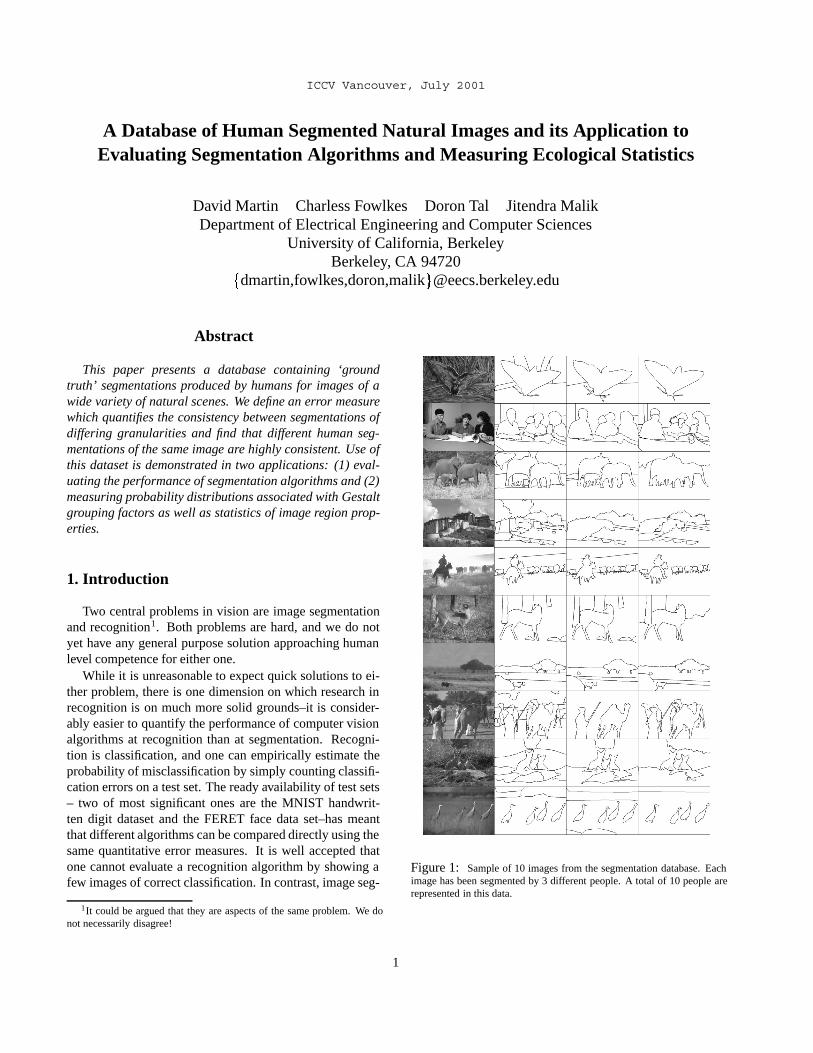
A Database of Human Segmented Natural Images and its ...fowlkes/papers/mftm-iccv01.pdf · Evaluating Segmentation Algorithms and Measuring Ecological ... mentations of the same image

ICCV Vancouver, July 2001

A Database of Human Segmented Natural Images and its Application toEvaluating Segmentation Algorithms and Measuring Ecological Statistics

David Martin Charless Fowlkes Doron Tal Jitendra MalikDepartment of Electrical Engineering and Computer Sciences

University of California, BerkeleyBerkeley, CA 94720

fdmartin,fowlkes,doron,[email protected]

Abstract

This paper presents a database containing ‘groundtruth’ segmentations produced by humans for images of awide variety of natural scenes. We define an error measurewhich quantifies the consistency between segmentations ofdiffering granularities and find that different human seg-mentations of the same image are highly consistent. Use ofthis dataset is demonstrated in two applications: (1) eval-uating the performance of segmentation algorithms and (2)measuring probability distributions associated with Gestaltgrouping factors as well as statistics of image region prop-erties.

1. Introduction

Two central problems in vision are image segmentationand recognition1. Both problems are hard, and we do notyet have any general purpose solution approaching humanlevel competence for either one.

While it is unreasonable to expect quick solutions to ei-ther problem, there is one dimension on which research inrecognition is on much more solid grounds–it is consider-ably easier to quantify the performance of computer visionalgorithms at recognition than at segmentation. Recogni-tion is classification, and one can empirically estimate theprobability of misclassification by simply counting classifi-cation errors on a test set. The ready availability of test sets– two of most significant ones are the MNIST handwrit-ten digit dataset and the FERET face data set–has meantthat different algorithms can be compared directly using thesame quantitative error measures. It is well accepted thatone cannot evaluate a recognition algorithm by showing afew images of correct classification. In contrast, image seg-

1It could be argued that they are aspects of the same problem. We donot necessarily disagree!

Figure 1: Sample of 10 images from the segmentation database. Eachimage has been segmented by 3 different people. A total of 10 people arerepresented in this data.

1

(a) (b) (c) (d)

Figure 2: Using the segmentation tool. See x2.1 for details.

(a) (b)

(c) (d)

Figure 3: Motivation for making segmentation error measures tolerantto refinement. (a) shows the original image. (b)-(d) show three segmen-tations in our database by different subjects. (b) and (d) are both simplerefinements of (c), while (b) and (d) illustrate mutual refinement.

mentation performance evaluation remains subjective. Typ-ically, researchers will show their results on a few imagesand point out why the results ‘look good’. We never knowfrom such studies whether the results are best examples ortypical examples, whether the technique will work only onimages that have no texture, and so on.

The major challenge is that the question “What is a cor-rect segmentation” is a subtler question than “Is this digita 5”. This has led researchers e.g. Borra and Sarkar[3]to argue that segmentation or grouping performance can beevaluated only in the context of a task such as object recog-nition. We don’t wish to deny the importance of evaluatingsegmentations in the context of a task. However, the the-sis of this paper is that segmentations can also be evaluatedpurely as segmentations by comparing them to those pro-duced by multiple human observers and that there is consid-erable consistency among different human segmentations ofthe same image so as to make such a comparison reliable.

Figure 1 shows some example images from the database

and 3 different segmentations for each image. The imagesare of complex, natural scenes. In such images, multiplecues are available for segmentation by a human or a com-puter program–low level cues such as coherence of bright-ness, texture or continuity of contour, intermediate levelcues such as symmetry and convexity, as well as high levelcues based on recognition of familiar objects. The instruc-tions to the human observers made no attempt to restrict orencourage the use of any particular type of cues. For in-stance, it is perfectly reasonable for observers to use theirfamiliarity with faces to guide their segmentation of the im-age in the second row of Figure 1. We realize that this im-plies that a computational approach based purely on, say,low-level coherence of color and texture, would find it dif-ficult to attain perfect performance. In our view, this is per-fectly fine. We wish to define a ‘gold standard’ for seg-mentation results without any prior biases on what cues andalgorithms are to be exploited to obtain those results. Weexpect that as segmentation and perceptual organization al-gorithms evolve to make richer use of multiple cues, theirperformance could continue to be evaluated on the samedataset.

Note that the segmentations produced by different hu-mans for a given image in Figure 1 are not identical. But,are they consistent? One can think of a human’s percep-tual organization as imposing a hierarchical tree structureon the image. Even if two observers have exactly the sameperceptual organization of an image, they may choose tosegment at varying levels of granularity. See e.g. Figure 3.This implies that we need to define segmentation consis-tency measures that do not penalize such differences. Wedemonstrate empirically that human segmentations for thewide variety of images in the database are quite consistentaccording to these criteria, suggesting that we have a re-liable standard with which to evaluate different computeralgorithms for image segmentation. We exploit this fact todevelop a quantitative performance measure for image seg-mentation algorithms.

There has been a limited amount of previous work evalu-ating segmentation performance using datasets with humanobservers providing the ground truth. Heath et al. [8] eval-uated the output of different edge detectors on a subjectivequantitative scale using the criterion of ease of recogniz-ability of objects (for human observers) in the edge images.Closer to our work is the Sowerby image dataset that hasbeen used by Huang [9] and Konishi et al. [12]. This datasetis small, not publicly available, and contains only one seg-mentation for each image. In spite of these limitations, thedataset has proved quite useful for work such as that of Kon-ishi et al. who used it to evaluate the effectiveness of dif-ferent edge filters as indicators of boundaries. We expectthat our dataset would find far wider use, by virtue of beingconsiderably more varied and extensive, and the fact that

2

0 0.2 0.4 0.6 0.8 10

20

40

60GCE measure (same images)

0 0.2 0.4 0.6 0.8 10

200

400

600

800

1000GCE measure (different images)

0 0.2 0.4 0.6 0.8 10

20

40

60LCE measure (same images)

0 0.2 0.4 0.6 0.8 10

200

400

600

800

1000LCE measure (different images)

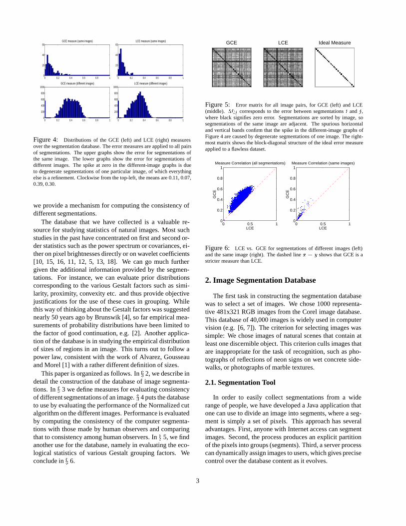
Figure 4: Distributions of the GCE (left) and LCE (right) measuresover the segmentation database. The error measures are applied to all pairsof segmentations. The upper graphs show the error for segmentations ofthe same image. The lower graphs show the error for segmentations ofdifferent images. The spike at zero in the different-image graphs is dueto degenerate segmentations of one particular image, of which everythingelse is a refinement. Clockwise from the top-left, the means are 0.11, 0.07,0.39, 0.30.

we provide a mechanism for computing the consistency ofdifferent segmentations.

The database that we have collected is a valuable re-source for studying statistics of natural images. Most suchstudies in the past have concentrated on first and second or-der statistics such as the power spectrum or covariances, ei-ther on pixel brightnesses directly or on wavelet coefficients[10, 15, 16, 11, 12, 5, 13, 18]. We can go much furthergiven the additional information provided by the segmen-tations. For instance, we can evaluate prior distributionscorresponding to the various Gestalt factors such as simi-larity, proximity, convexity etc. and thus provide objectivejustifications for the use of these cues in grouping. Whilethis way of thinking about the Gestalt factors was suggestednearly 50 years ago by Brunswik [4], so far empirical mea-surements of probability distributions have been limited tothe factor of good continuation, e.g. [2]. Another applica-tion of the database is in studying the empirical distributionof sizes of regions in an image. This turns out to follow apower law, consistent with the work of Alvarez, Gousseauand Morel [1] with a rather different definition of sizes.

This paper is organized as follows. In x 2, we describe indetail the construction of the database of image segmenta-tions. In x 3 we define measures for evaluating consistencyof different segmentations of an image. x 4 puts the databaseto use by evaluating the performance of the Normalized cutalgorithm on the different images. Performance is evaluatedby computing the consistency of the computer segmenta-tions with those made by human observers and comparingthat to consistency among human observers. In x 5, we findanother use for the database, namely in evaluating the eco-logical statistics of various Gestalt grouping factors. Weconclude in x 6.

GCE LCE Ideal Measure

Figure 5: Error matrix for all image pairs, for GCE (left) and LCE(middle). Mij corresponds to the error between segmentations i and j,where black signifies zero error. Segmentations are sorted by image, sosegmentations of the same image are adjacent. The spurious horizontaland vertical bands confirm that the spike in the different-image graphs ofFigure 4 are caused by degenerate segmentations of one image. The right-most matrix shows the block-diagonal structure of the ideal error measureapplied to a flawless dataset.

0 0.5 10

0.2

0.4

0.6

0.8

1

LCE

GC

E

Measure Correlation (all segmentations)

0 0.5 10

0.2

0.4

0.6

0.8

1

LCE

GC

E

Measure Correlation (same images)

Figure 6: LCE vs. GCE for segmentations of different images (left)and the same image (right). The dashed line x = y shows that GCE is astricter measure than LCE.

2. Image Segmentation Database

The first task in constructing the segmentation databasewas to select a set of images. We chose 1000 representa-tive 481x321 RGB images from the Corel image database.This database of 40,000 images is widely used in computervision (e.g. [6, 7]). The criterion for selecting images wassimple: We chose images of natural scenes that contain atleast one discernible object. This criterion culls images thatare inappropriate for the task of recognition, such as pho-tographs of reflections of neon signs on wet concrete side-walks, or photographs of marble textures.

2.1. Segmentation Tool

In order to easily collect segmentations from a widerange of people, we have developed a Java application thatone can use to divide an image into segments, where a seg-ment is simply a set of pixels. This approach has severaladvantages. First, anyone with Internet access can segmentimages. Second, the process produces an explicit partitionof the pixels into groups (segments). Third, a server processcan dynamically assign images to users, which gives precisecontrol over the database content as it evolves.

3

Figure 2 shows a sequence of snapshots taken from atypical session with the segmentation tool. Each snapshotshows two windows. The upper window is the main win-dow of the application. It shows the image with all segmentsoutlined in white. The lower window in each snapshot is thesplitter window, which is used to split an existing segmentinto two new segments.

Consider Figure 2(a). The main window shows two seg-ments. The user has selected the larger one in order to splitit using the lower window. Between (a) and (b), the userdrew a contour around the leftmost two pups in the top paneof the splitter window. This operation transfers the enclosedpixels to the bottom pane, creating a new segment. Between(c) and (d), the user split the two pups from each other. In(d), there are 4 segments.

In addition to simply splitting segments, the user cantransfer pixels between any two existing segments. Thisprovides a tremendous amount of flexibility in the way inwhich users create and define segments. The interface issimple, yet accommodates a wide range of segmentationstyles. In less than 5 minutes, one can create a high-quality,pixel-accurate segmentation with 10-20 segments using astandard PC.

2.2. Experiment Setup and Protocol

It is imperative that variation among human segmenta-tions of an image is due to different perceptual organiza-tions of the scene, rather than aspects of the experimentalsetup. In order to minimize variation due to different inter-pretations of the task, the instructions were made intention-ally vague in an effort to cause the subjects to break up thescene in a “natural” manner: Divide each image into pieces,where each piece represents a distinguished thing in the im-age. It is important that all of the pieces have approximatelyequal importance. The number of things in each image is upto you. Something between 2 and 20 should be reasonablefor any of our images.

The initial subject group was a set of students in agraduate-level computer vision class who were additionallyinstructed to segment as naive observers. The subjects wereprovided with several example segmentations of simple, un-ambiguous images as a visual description of the task.

Images were assigned to subjects dynamically. When asubject requested a new image, an image was chosen ran-domly with a bias towards images that had been segmentedby some other subject. In addition, the software ensuredthat (1) no subject saw the same image twice, (2) no im-age was segmented by more than 5 people, and (3) no twoimages were segmented by exactly the same set of subjects.

Figure 7: Segmentations produced by the Normalized Cuts algorithmusing both contour and texture cues. Compare with Figure 1.

0 0.2 0.4 0.6 0.8 10

20

40

60GCE measure (same images)

0 0.2 0.4 0.6 0.8 10

200

400

600

800

1000GCE measure (different images)

0 0.2 0.4 0.6 0.8 10

20

40

60LCE measure (same images)

0 0.2 0.4 0.6 0.8 10

200

400

600

800

1000LCE measure (different images)

Figure 8: Distributions of the GCE (left) and LCE (right) measures forNCuts segmentations vs. human segmentations. The error measures wereapplied to pairs of segmentations, where each pair contains one NCuts andone human segmentations (see x4 for details). The upper graphs show theerror for segmentations of the same image. For reference, the lower graphsshow the error for segmentations of different images. Clockwise from thetop-left, the means are 0.28, 0.22, 0.38, 0.31. Compare with Figure 4.

2.3. Database Status and Plans

The results in this paper were generated using our firstversion of the dataset that contains 150 grayscale segmen-tations by 10 people of 50 images, with 30 images with 3 ormore segmentations. The data collection is ongoing, and atthis time, we have 3000 segmentations by 25 people of 800images. We aim to ultimately collect at least 4 grayscaleand 4 color segmentations of 1000 images.

3. Segmentation Error Measures

There are two reasons to develop a measure that pro-vides an empirical comparison between two segmentationsof an image. First, we can use it to validate the segmen-tation database by showing that segmentations of the sameimage by different people are consistent. Second, we can

4

1 3 5 7 9 11 13 15 17 19 21 23 25 27 290

0.1

0.2

0.3

0.4

0.5

0.6

0.7

0.8

0.9

1Er

ror

Image Number

Figure 9: The GCE for human vs. human (gray) and NCuts vs. human(white) for each image for which we have � 3 human segmentations. TheLCE data is similar.

use the measure to evaluate segmentation algorithms in anobjective manner.

A potential problem for a measure of consistency be-tween segmentations is that there is no unique segmenta-tion of an image. For example, two people may segment animage differently because either (1) they perceive the scenedifferently, or (2) they segment at different granularities. Iftwo different segmentations arise from different perceptualorganizations of the scene, then it is fair to declare the seg-mentations inconsistent. If, however, one segmentation issimply a refinement of the other, then the error should besmall, or even zero. Figure 3 shows examples of both sim-ple and mutual refinement from our database. We do not pe-nalize simple refinement in our measures, since it does notpreclude identical perceptual organizations of the scene.

In addition to being tolerant to refinement, any errormeasure should also be (1) independent of the coarsenessof pixelation, (2) robust to noise along region boundaries,and (3) tolerant of different segment counts between the twosegmentations. The third point is due to the complexity ofthe images: We need to be able to compare two segmenta-tions when they have different numbers of segments. In theremainder of this section, we present two error measuresthat meet all of the aforementioned criteria. We then applythe measures to the database of human segmentations.

3.1. Error Measure Definitions

A segmentation is simply a division of the pixels of animage into sets. A segmentation error measure takes twosegmentations S1 and S2 as input, and produces a real-valued output in the range [0::1] where zero signifies noerror.

We define a measure of error at each pixel that is tolerantto refinement as the basis of both measures. For a givenpixel pi consider the segments in S1 and S2 that contain

that pixel. The segments are sets of pixels. If one segmentis a proper subset of the other, then the pixel lies in an areaof refinement, and the local error should be zero. If thereis no subset relationship, then the two regions overlap in aninconsistent manner. In this case, the local error should benon-zero. Let n denote set difference, and jxj the cardinalityof set x. If R(S; pi) is the set of pixels corresponding to theregion in segmentation S that contains pixel p i, the localrefinement error is defined as:

E(S1; S2; pi) =jR(S1; pi)nR(S2; pi)j

jR(S1; pi)j(1)

Note that this local error measure is not symmetric. Itencodes a measure of refinement in one direction only:E(S1; S2; pi) is zero precisely when S1 is a refinement ofS2 at pixel pi, but not vice versa. Given this local refinementerror in each direction at each pixel, there are two naturalways to combine the values into a error measure for the en-tire image. Global Consistency Error (GCE) forces all localrefinements to be in the same direction. Local ConsistencyError (LCE) allows refinement in different directions in dif-ferent parts of the image. Let n be the number of pixels:

GCE(S1; S2) =1

nmin

(Xi

E(S1; S2; pi);

Xi

E(S2; S1; pi)

)(2)

LCE(S1; S2) =1

n

Xi

min�E(S1; S2; pi);

E(S2; S1; pi)

(3)

As LCE � GCE for any two segmentations, it is clearthat GCE is a tougher measure than LCE. Looking at Fig-ure 3, GCE would tolerate the simple refinement from (c)to (b) or (d), while LCE would also tolerate the mutualrefinement of (b) and (d). Note that since both measuresare tolerant of refinement, they are meaningful only whencomparing two segmentations with an approximately equalnumber of segments. This is because there are two trivialsegmentations that achieve zero error: One pixel per seg-ment, and one segment for the entire image. The former isa refinement of any segmentation, and any segmentation isa refinement of the latter.

3.2. Error Measure Validation

We apply the GCE and LCE measures to all pairs of seg-mentations in our dataset with two goals. First, we hope toshow that given the arguably ambiguous task of segmentingan image into an unspecified number of segments, differentpeople produce consistent results on each image. Second,we hope to validate the measures by showing that the error

5

between segmentations of the same image is low, while theerror between segmentations of different images is high.

Figure 4 shows the distribution of error between pairs ofhuman segmentations. The top graphs show the error be-tween segmentations of the same image; the bottom graphsshow the error between segmentations of different images.As expected, the error distribution for segmentations of thesame image shows a strong spike near zero, while the errordistribution for segmentations of different images is neitherlocalized nor close to zero.

We characterize the separation of the two distributionsby noting that for LCE, 5.9% of segmentation pairs lieabove 0.12 for the same image or below 0.12 for differentimages. For GCE, 5.9% of pairs lie above 0.16 for the sameimage or below 0.16 for different images. Note the goodbehavior of both measures despite the fact that the numberof segments in each segmentation of a particular image canvary by a factor of 10. Figure 5 shows the raw data used tothe compute the histograms.

In Figure 6, we plot LCE vs. GCE for each pair of seg-mentations. As expected, we see (1) that GCE and LCE aremeasuring similar qualities, and (2) that GCE > LCE in allcases.

4. A Segmentation Benchmark

In this section, we use the segmentation database and er-ror measures to evaluate the Normalized Cuts (NCuts) im-age segmentation algorithm.

In collecting our dataset, we permitted a great deal offlexibility in how many segments each subject created for animage. This is desirable from the point of view of creatingan information-rich dataset. However, when comparing ahuman segmentation to a computer segmentation, our mea-sures are most meaningful when the number of segmentsis approximately equal. For example, an algorithm couldthwart the benchmark by producing one segment for thewhole image, or one segment for each pixel. Due to thetolerance of GCE and LCE to refinement, both of these de-generate segmentations have zero error.

Since image segmentation is an ill-posed problem with-out stating the desired granularity, we can expect any seg-mentation algorithm to provide some sort of control overthe number of segments it produces. If our human segmen-tations of an image contain 4, 9, and 13 segments, then weinstruct the computer algorithm to also produce segmenta-tions with 4, 9, and 13 segments. We then compare eachcomputer segmentation to each human segmentation. In thisway, we can make a meaningful comparison to the humansegmentation error shown in Figure 4. In addition, we con-sider the mean error over all images as a summary statisticthat can be used to rank different segmentation algorithms.

The NCuts algorithm [17, 14] takes a graph theoretic ap-

0 0.2 0.4 0.6 0.8 10

0.1

0.2

0.3

0.4

0.5

0.6

0.7

0.8

0.9

1P(samesegment|distance)

distance (normalized)

prob

abili

ty o

f sam

e se

gmen

t

Figure 10: Proximity: The probability that two points belong to thesame segment given their distance. Distances have been scaled per imageas discussed in the text and normalized to range from 0 to 1. We sample1000 points from each segmentation and compute all pairwise distances.Error bars show �� intervals.

proach to the problem of image segmentation. An imageis treated as a weighted graph. Each pixel corresponds toa node, and edge weights computed from both contour andtexture cues denote a local measure of similarity betweentwo pixels. NCuts segments an image by cutting this graphinto strongly connected parts. The version of NCuts de-scribed in [14] automatically determines the number of re-gions by splitting the graph until the cuts surpass a thresh-old. We modified the stopping criterion to provide explicitcontrol over the final number of segments.

Figure 8 shows the error between NCuts segmentationsand human segmentations. In comparing this NCuts errorto the human error shown in Figure 4, we see that NCuts isproducing segmentations worse than humans, but still betterthan “random.” The error distributions for segmentations ofdifferent images (the bottom graphs in each figure) approx-imate the performance of random segmentation. The meanerror over all segmentation pairs gives NCuts an overall er-ror of 22% by LCE (compared to 7% for humans), and 28%by GCE (compared to 11% for humans).

Figure 9 shows both the human error (blue) and NCutserror (red) for each image separately. In most cases, thehuman segmentations form a tight distribution near zero. Invirtually all cases, NCuts performs worse than humans, butit fares better on some images than others. This data can beused to find the type of images for which an algorithm hasthe most difficulty.

5. Bayesian Interpretation of Gestalt GroupingFactors

Brunswik [4] suggested that the various Gestalt factorsof grouping such as proximity, similarity, convexity, etc.made sense because they reflected the statistics of naturalscenes. For instance, if nearby pixels are more likely to

6

0 0.1 0.2 0.3 0.4 0.5 0.6 0.7 0.8 0.9 10

0.1

0.2

0.3

0.4

0.5

0.6

0.7

0.8

0.9

1P(samesegment|intensitydif)

intensity differnece (normalized)

prob

abili

ty o

f sam

e se

gmen

t

Figure 11: Similarity: The probability that two points belong to thesame segment given their absolute difference in intensity (256 gray levels).We sample 1000 points from each segmentation and compute all pairwisesimilarities. Error bars show �� intervals.

belong to the same region, it is justified to group them.In computer vision, we would similarly like grouping al-gorithms to be based on these ecological statistics. TheBayesian framework provides a rigorous approach to ex-ploiting this knowledge in the form of prior probability dis-tributions. Our database enables the empirical measurementof these distributions.

In this section, we present our measurements of theprobability distributions associated with the Gestalt cues ofproximity, similarity of intensity, and convexity of regions.As another interesting empirical finding, we determine thefrequency distribution of region areas and show that it fol-lows a power law.

5.1. Proximity Cues

Experiments have long shown that proximity is an im-portant low-level cue in deciding how stimuli will begrouped. We characterize this cue by estimating the prob-ability that two points in an image will lie in the same re-gion given their distance on the image plane. The resultsare summarized in the form of a histogram where eachbin counts the proportion of point-pairs in a given distancerange that lie within the same segment as designated by thehuman segmentor. We would like our estimate to be in-variant to the granularity at which a particular image hasbeen segmented. To this end, we scale all distances byq

number of segmentsimage area .

Results are show in Figure 10. As might be expected theprobability of belonging to the same group is one when thedistance is zero and decreases monotonically with increas-ing distance.

5.2. Similarity Cues

Using a similar methodology to x5.1, we examine theprobability that two points lie in the same region given their

0 0.1 0.2 0.3 0.4 0.5 0.6 0.7 0.8 0.9 10

20

40

60

80

100

120

140

160

frequency of convexity measure

convexity

num

ber

of o

ccur

ance

s

Figure 12: Convexity: The distribution of the convexity of segments.Convexity is measured as ratio of a region’s area to the area of its convexhull yielding a number between 0 and 1. Error bars show �� intervals.

similarity. We evaluate point-wise similarity based on theabsolute difference in pixel intensity (256 gray levels). Thiscould be clearly be extended to make use of color or localtexture. The results are shown in Figure 11. If images of ob-jects were uniform in intensity over the extent of the objectwith some additive noise and each object in a given scenehad a unique intensity, we would expect to see a curve thatstarted at 1 and quickly decayed to 0. However, images ofnatural objects feature variation in intensity due to texture,shading, and lighting so the histogram we compute startsat 0.6 and monotonically decays to 0.2. This suggests thatalthough similarity in intensity isn’t a perfect cue, it doescapture some useful information about group membership.

5.3. Region Convexity

One commonly posited mid-level grouping cue is theconvexity of foreground object boundaries. We capturethe notion of convexity for discrete, pixel-based regions bymeasuring the ratio of a region’s area to the area of its con-vex hull. This yields a number between zero and one whereone indicates a perfectly convex region. Since the regionsin our dataset have no labels that designate them as fore-ground or background we are forced to look at the distribu-tion of the convexity of all image regions. This on its own isarguably instructive and we imagine that since there can bemany foreground groups and only a few background groupsin a given image, the distribution for only foreground re-gions would look very similar. Figure 12 shows our results.As expected, grouped pixels commonly form a convex re-gion.

5.4. Region Area

The authors of [1] approach the problem of estimatingthe distribution of object sizes in natural imagery by au-tomatically finding connected components of bilevel setsand fitting the distribution of their areas. Our results from

7

103

104

105

10−3

10−2

10−1

100

region area

num

ber

of o

ccur

ance

s

frequency of region area

Figure 13: Region Area: This log-log graph shows the distribution inregion areas. We fit a curve of the form y =

Ax�

yielding an � = 1:008.For the purposes of fitting, we throw out those sparsely populated binswhich contain regions that are greater than 25% of the total image area.

x5.2 suggest that intensity bilevel sets are only a rough ap-proximation to perceptual segments in the image. Figure 13shows the distribution of region areas in our data set. We getan excellent fit from a power law curve of the form y = A

x�

yielding an � = 1:008.

6. Summary and Conclusion

In this paper, we presented a database of natural imagessegmented by human subjects along with two applicationsof the dataset. First, we developed an image segmentationbenchmark by which one can objectively evaluate segmen-tation algorithms. Second, we measured ecological statis-tics related to Gestalt grouping factors. In time, we expectthe database to grow to cover 1000 images, with 4 humansegmentations of each image in both grayscale and color.This data is to be made available to the community in thehope that we can place the problem of image segmentationon firm, quantitative ground.

Acknowledgments

We would like to thank Dave Patterson for his valu-able input, particularly in the data collection and bench-mark portions of this paper. We also graciously thank theFall 2000 students of UCB CS294, who provided our im-age segmentations. This work was supported in part by theUC Berkeley MICRO Fellowship (to CF), the NIH Train-ing Grant in Vision Science T32EY 07043-22 (to DT), AROcontract DAAH04-96-1-0341, the Digital Library grant IRI-9411334, Defense Advanced Research Projects Agency ofthe Department of Defense contract DABT63-96-C-0056,the National Science Foundation infrastructure grant EIA-9802069, and by a grant from Intel Corporation. The infor-

mation presented here does not necessarily reflect the po-sition or the policy of the Government and no official en-dorsement should be inferred.

References

[1] L. Alvarez, Y. Gousseau, and J. Morel. Scales in naturalimages and a consequence on their bounded variation norm.In Scale-Space Theories in Computer Vision, 1999.

[2] J. August and S. Zucker. The curve indicator random field:Curve organization via edge correlation. In K. L. Boyer andS. Sarkar, editors, Perceptual Organization in Artificial Vi-sion Systems, pages 265–287. Kluwer, 2000.

[3] S. Borra and S. Sarkar. A framework for performance char-acterization of intermediate-level grouping modules. PAMI,19(11):1306–1312, Nov. 1997.

[4] E. Brunswik and J. Kamiya. Ecological validity of proximityand other gestalt factors. Am. J. of Psych., pages 20–32,1953.

[5] R. W. Buccigrossi and E. P. Simoncelli. Image compressionvia joint statistical characterization in the wavelet domain.IEEE Trans. on Image Proc., 8(12):1688–1701, Dec. 1999.

[6] C. Carson, M. Thomas, S. Belongie, J. M. Hellerstein, andJ. Malik. Blobworld: A system for region-based image in-dexing and retrieval. Third International Conference on Vi-sual Information Systems, Jun. 1999.

[7] O. Chapelle, P. Haffner, and V. N. Vapnik. Support vectormachines for histogram-based image classification. IEEETrans. on Neural Networks, 10(5):1055–1064, Sep. 1999.

[8] M. D. Heath, S. Sarkar, T. Sanocki, and K. W. Bowyer. A ro-bust visual method for assessing the relative performance ofedge-detection algorithms. PAMI, 19(12):1338–1359, 1997.

[9] J. Huang. Statistics of Natural Images and Models. PhDthesis, Brown University, May 2000.

[10] J. Huang, A. B. Lee, and D. Mumford. Statistics of rangeimages. CVPR, pages 324–331, 2000.

[11] J. Huang and D. Mumford. Statistics of natural images andmodels. CVPR, pages 541–547, 1999.

[12] S. Konishi, A. L. Yuille, J. Coughlan, and S. C. Zhu. Funda-mental bounds on edge detection: an information theoreticevaluation of different edge cues. CVPR, pages 573–579,1999.

[13] A. B. Lee and D. Mumford. Scale-invariant random-collagemodel for natural images. In Proc. IEEE Workshop on Sta-tistical and Computational Theories of Vision. 1999.

[14] J. Malik, S. Belongie, T. Leung, and J. Shi. Contour and im-age analysis for segmentation. In K. L. Boyer and S. Sarkar,editors, Perceptual Organization for Artificial Vision Sys-tems, pages 139–172. Kluwer, 2000.

[15] D. L. Ruderman. The statistics of natural images. Network,5(4):517–548, 1994.

[16] D. L. Ruderman. Origins of scaling in natural images. VisionResearch, 37:3385–3395, 1997.

[17] J. Shi and J. Malik. Normalized cuts and image segmenta-tion. PAMI, 22(8):888–905, Aug. 2000.

[18] J. H. van Hateren and A. V. der Schaaf. Independent com-ponent filters of natural images compared with simple cellsin primary visual cortex. Proc. R. Soc. Lond., 265:359–366,1998.

8