A Data Locating Mechanism for Distributed XML Data over ...

A Data Locating Mechanism for Distributed XML Data over P2P

Networks ∗

Qiang Wang AND M. Tamer Ozsu

University of Waterloo

School of Computer Science

Waterloo, Canada

{q6wang,tozsu}@uwaterloo.ca

Technical Report CS-2004-45 Oct. 2004

∗submitted to ICDCS 2005

1

Abstract

Many emerging applications that use XML are distributed, usually over the Internet or over large

Peer-to-Peer (P2P) networks. A fundamental problem of XML query processing in these systems is how

to locate the data relevant to the queries so that only useful data are involved in query evaluation. In this

paper, we address this problem within the context of structured P2P networks, and propose a novel data

locating mechanism for query shipping systems. Our approach follows the multi-hop routing approach

and encodes the hierarchical information of the XML data into the overlay network, so that routing

keys can be hierarchical XML path expressions. We also propose a decentralized data locating algorithm

that does not employ a centralized catalog but also avoids flooding the network with XML queries. We

report comprehensive experiments to demonstrate the scalability and effectiveness of the data locating

mechanism.

1 Introduction

In recent years, Peer-to-Peer (P2P) distribution architecture has become a popular decentralized platform for

many Internet-scale applications such as file sharing1, instant messaging2, and computing resource sharing3.

Meanwhile, XML is being increasingly used as a data format for data exchange and storage on the Internet.

Many of the XML data repositories are distributed. For example, sensor data in XML format are stored

geographically close to the sensors [14], large XML documents are partitioned and allocated to distributed

physical sites [11], and XML-based descriptions in WSDL [8] and SOAP [9] provide interfaces for distributed

Web services. Although there exist some work on distributed XML query processing (e.g. [27]), we are faced

with new challenges when XML data are deployed over large-scale P2P networks, where centralized catalogs

are not available and peers may join and leave arbitrarily.

Consider, as an example, peer services in a self-organized P2P community, where services are pro-

vided such as book sharing and carpooling. We assume that each peer service publishes the informa-

tion about the available books or carpooling using simple XML paths shown in Figure 1. Alternatively,

Web service description languages such as WSDL and SOAP can be used, but we don’t consider that

approach in this paper. Another assumption of this work is that each peer is aware of the schema on

which queries are executed. Note that multiple schemas (e.g. one schema for each peer service) may

exist in the P2P network and XML queries can be issued at any peer. For example, the query “/PeerSer-

vice/Country[@name=‘Canada’]/Province[@name=‘Ontario’]/City[@name=‘Waterloo’] /Carpooling[date =

‘2004 Dec.19’]” can be issued by a peer in the network to retrieve all carpooling service data provided in the

city of Waterloo on the specified date. Besides Web services, many other distributed XML query processing

systems fit a similar computation model, e.g. distributed XML repositories [11] over P2P networks.

A fundamental problem for distributed query processing is how to locate the data relevant to the queries so

that only useful data are involved in the query execution. This is crucial for large-scale network environments

such as the Internet-scale P2P networks where the network communication cost of transferring data and

queries dominates the performance of the system. A number of approaches to the problem have been

proposed. Data may be located by looking up the information in DNS (Domain Name Service) style catalogs

[14]. However, such an approach assumes DNS servers to be stable, which is not guaranteed in a P2P network

1Gnutella http://www.gnutella.com2Skype http://www.skype.com3Seti@home http://setiathome.ssl.berkeley.edu

2

Book sharing:

/PeerService[@provider=‘Jane’]/Country[@name=‘United States’]/State[@name=‘New York’]

[@region=‘Northeast’]/City[@name=‘Boston’]/Book[@name=‘Road Worthy’]

Carpooling service:

/PeerService[@provider=‘John’]/Country[@name=‘Canada’]/Province[@name=‘Ontario’]/City

[@name=‘Waterloo’]/Carpooling[@via=‘Toronto’][@date=‘2004 Dec.19’]

Figure 1: Peer service descriptions

where peers may join or leave the network arbitrarily. Another approach is to fully replicate global catalog

information on all peers so that each peer knows exactly where the relevant data reside for the queries [11].

Obviously, this approach does not scale in an Internet-scale distributed system. Finally, in a generalized

P2P network environment, we do not assume the employment of centralized mechanisms such as superpeers

employed by P2P file sharing systems, e.g. KaZaA4.

In this paper, we design a novel data locating mechanism for distributed XML query processing over P2P

networks that is based on a purely decentralized catalog service and a multi-hop routing mechanism. More

specifically, to avoid a centralized catalog service, we encode the hierarchical information of the distributed

XML data on each peer into a specially-designed overlay network so that each peer manages part of the

catalog information. Based on the decentralized catalog information, a peer can be reached through a multi-

hop routing mechanism according to the path of the data published by that peer. For simple queries targeted

to one peer, the query can be sent over to the peer by routing directly, while for complex queries covering

several peers, the propagation of the query is inevitable. To avoid flooding the overlay network, we first

route the query to a logical rendezvous node from where it is propagated within a sub-network to locate the

relevant data. This approach is similar, in some sense, to IP multicast strategy.

There are similarities between our work and structured P2P file sharing systems (e.g. Chord [26], CAN

[22], Pastry [24], and Tapestry [29]), whose primary goal is to decentralize the catalog service and rout-

ing mechanism so as to locate the files efficiently over large-scale dynamic networks without flooding the

network with the queries or employing specialized peers for catalog service. The main idea behind these

structured P2P file sharing systems is to build overlay networks consisting of logical nodes derived from

the file names and impose some relationships among the logical nodes to facilitate the file locating pro-

cess. It has been proven both theoretically and experimentally that these systems are highly scalable over

Internet-scale networks, and can deal with the frequent changes of the network environments, i.e. the joining

and leaving of the peers. Although we exploit the idea of overlay networks and routing ideas developed

for P2P file sharing systems, our work differs from them in important ways. The P2P file sharing systems

only support a flat routing key (e.g. file names) rather than the hierarchically structured ones as exist in

XML path expressions defined in XPath language [13] that is also embedded in XQuery [10]. For example,

the query “/PeerService/Country[@name=‘Canada’]//City[@name=‘Waterloo’] /Carpooling[date = ‘2004

Dec.19’]” contains hierarchical constructs such as parent-child axis and ancestor-descendant axis. The most

likely approach for P2P file sharing systems to resolve the XML data locating is to treat the whole query

expression as a flat key, which means that a query can only locate the distributed XML data with an ex-

actly matching path expression. Alternatively, P2P file sharing systems can deal with XML data locating4KaZaA http://www.kazaa.com

3

by separating the data locating process on the flat names from the one on the hierarchical constructs [17].

Because of the separation, the matching of the queries against the distributed XML data on the hierarchical

constructs still employs some centralized mechanism, which leads to performance degradation and scalability

problems. To solve these problems, we integrate the matching process on the hierarchical constructs directly

into the decentralized catalog management and routing mechanism by designing an overlay network where

the hierarchical information of the distributed XML data is encoded. To the best of our knowledge, ours is

the first design that follows this approach.

In brief, our data locating mechanism can be highlighted as follows:

1. We avoid any centralized management of the catalog and adopt a purely decentralized mechanism,

where each peer keeps a part of the catalog information. Furthermore, catalog management is based

on a specially designed overlay network which encodes the hierarchical structure information of all

the distributed XML data. The overlay network consists of logical nodes, each corresponding to a

unique XML path expression published by peers, as shown in Figure 1. The relationship among the

logical nodes is built according to the hierarchical structure information contained in the XML path

expressions. This novel way of encoding hierarchical information of distributed XML data into the

overlay network greatly reduces the size of the catalog information. Moreover, the updates on the

catalog information, which are very common in a P2P system, can now be managed in a decentralized

way. Based on the decentralized catalog management, we design a multi-hop routing algorithm that

can reach an arbitrary peer through the paths published by that peer (e.g. Figure 1).

2. The data locating mechanism supports a declarative query language which captures the essential nav-

igational constructs of the XPath language. The data locating mechanism rewrites a declarative XML

query into either a process of routing towards a specific logical node in the overlay network or a process

of propagating the query within a limited part of the overlay network so as to locate all the peers con-

taining the relevant data. Consequently, our approach avoids flooding the network or using DNS-style

servers.

To evaluate the effectiveness of the data locating mechanism, we deploy synthetic distributed XML data

over a simulated P2P network generated using NS-2 [5] in transit-stub topology, and we take measurements

on several metrics related to the overlay network and different kinds of XML queries. Experimental results

demonstrate good scalability.

The organization of the paper is as follows. The related work is presented in Section 2. Section 3

introduces the preliminary knowledge including the definition of the distributed XML data and the overlay

network. Based on the overlay network, a decentralized catalog management and a decentralized multi-

hop routing mechanism are discussed, respectively, in Sections 4 and 5. In Section 6, the data locating

mechanism for declarative XML queries is addressed. In Section 7 we discuss the impact on our mechanism

of the frequent joining and leaving of the peers on our mechanism. Section 8 is focused on a series of

experiments for performance evaluation. Finally we conclude in Section 9.

2 Related Work

Galanis et al. [17] also address the problem of locating relevant data for XML queries. They propose

an approach that uses a two-phase process: in the first phase, a specific element name contained in the

4

XML queries is used as the routing key to locate a catalog that includes the physical site information of all

the distributed XML data containing the elements with that name. This phase is realized using existing

structured P2P routing mechanisms (e.g. Chord) because the routing keys are just flat-structured element

names. In the second phase, the path descriptions of the distributed XML data in the catalog are matched

against queries, and the physical sites containing the relevant data are located. Since the catalog information

is not evenly distributed among the distributed physical sites, some sites may become bottleneck when a

vast number of queries are targeted at them. Another problem is that the path description information is

replicated among the catalog sites corresponding to the names contained in the path descriptions, which adds

extra overhead for consistency maintenance. In contrast, we encode the hierarchical structure information

into the overlay network, consequently each distributed catalog can exclude the structure information and

manage much less information. Furthermore, since the distributed XML data cluster according to their

hierarchical structure in the overlay network, it is especially efficient to locate the relevant data for queries

containing the hierarchical constructs such as ancestor-descendant axis and wild cards, which aggregate

structurally similar distributed XML data.

There are other works addressing distributed XML processing. Deshpande et al. discuss distributed

XML processing in a sensor database [14], where the distributed XML data are stored geographically close

to sensors, and DNS-style servers are employed to locate all physical sites containing data relevant to a

query. The Active XML project [1] defines a P2P framework to integrate XML-based Web services, where

an Active XML document embeds calls for services distributed on different physical sites. Since the services

are referenced using the physical sites’ domain names or IP addresses, relevant data are located directly

through DNS services on the Internet. We avoid specialized servers in our design by decentralizing the

catalog information among all the peers. Similar to DNS style catalogs, XML dissemination systems (e.g.

[15]) employ a technique which aggregates the routing information on several distributed brokers based on

the topology of a broadcast tree. The aggregation technique is also employed by Koloniari et al. [19], where

summary information on each peer is aggregated on ancestor peers following a hierarchical organization. The

problem with this approach is that the routing information is replicated along the routing tree, substantially

increasing the consistency maintenance cost.

Bremer et al. [11] focus on a top-down design methodology of distributed XML repository systems,

whereby large XML documents are partitioned and allocated to distributed physical sites. In their design,

the catalog information is fully replicated to all distributed physical sites so that each one is aware of all the

mapping information between the fragment data and the physical sites. We, on the other hand, require each

peer to only manage a small amount of catalog information, improving scalability.

Suciu addresses the query processing problems on distributed semistructured data [27]. The queries are

sent to all distributed nodes and partial query results are collected. As pointed out in the paper, this work

is only targeted at a small-scale network environment consisting of dozens of distributed physical sites.

Since we employ a multi-dimensional coordinate space to encode the hierarchical structure information

of the distributed XML data into the overlay network, another related work is the construction of the multi-

dimensional space for an XML path expression by mapping the element names on each level of the path

expression to values [20]. In addition to the element names, we treat attribute values in the same way.

Furthermore, we use a secure hash function (i.e. SHA-1 [28]) for the mapping rather than a signature file

[21], because SHA-1 is recognized to have good distribution properties such as the guarantee of an even

distribution of the information in the overlay network [26].

5

3 Preliminaries

3.1 Distributed XML Data Definition

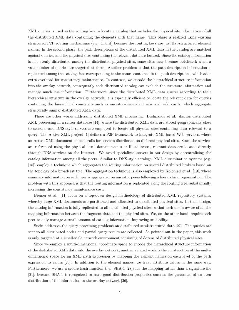
In this work, we use a simple XML path language to define distributed XML data deployed on each peer,

whose formal definition is shown in Figure 2. “Label” represents valid element or attribute names in XML

documents; “Number” and “String” represent numeric data and character string data respectively. For sim-

plicity of presentation, we do not include XML text nodes in this paper and an extension is straightforward.

Path ::= ‘/’ Steps

Steps ::= Step ‘/’ Step

Step::=Label (‘[’ Predicate ‘]’)*

Predicate ::= NumPred | StrPred

NumPred ::= ‘@’Label [‘=’ | ‘>’ | ‘<’ | ‘>=’ | ‘<=’] Number

StrPred ::= ‘@’Label ‘=’ String

Figure 2: Distributed XML data definition language

There are several other definitions of distributed XML data and XML fragment in literature, some used

for data exchange [16, 18], while others used for storage of distributed XML repositories [11]. Our distributed

XML data definition is simpler than these and is restricted to parent-child axis and relational predicates over

attributes. Our definition does not include ancestor-descendant axis, wild card, or the exclusion operation

(“-”) which can calculate the difference of two fragments as a new fragment [11]. There are multiple reasons

for using this simple language. First, there are existing distributed XML data that can be captured by this

language (e.g. the XML sensor data [14]). Second, this restricted language is a fundamental part of any XML

path language, thus it can be used as a building block of more complex definitions as in the top-down design

of distributed XML processing systems [11]. Third, the simplicity of the language indicates the possibility

of efficient manipulations over distributed data, which is obviously important for the overall performance of

the system.

A piece of distributed XML data on a peer can be published with the path expression defined using

the language, and one peer can publish multiple path expressions for different data. For example, in the

peer service example, two paths about service data, i.e. “/PeerService[@provider=‘John’]/Country[@name

=‘Canada’]/Province[@name =‘Ontario’]/City[@name =‘Toronto’]/Carpooling[@via =‘Toronto’][@date =

‘2004 Dec.19’]” and “/PeerService[@provider=‘John’]/Country[@name =‘Canada’]/Province[@name =‘On-

tario’]/City[@name =‘Toronto’]/Carpooling[@via =‘Kingston’][@date = ‘2004 Dec.22’]” can be published

by the same peer. Such path expressions can be extracted from the distributed XML data, e.g. in the

peer service case, or directly deployed by the data provider, e.g. in the distributed XML repository case.

For the latter case, fragments are computed by partitioning the original XML document in the repository

horizontally and vertically [11], where, in the context of distributed XML repository, horizontal partitioning

refers to a partition over the attribute values while vertical partitioning refers to a partition over rooted

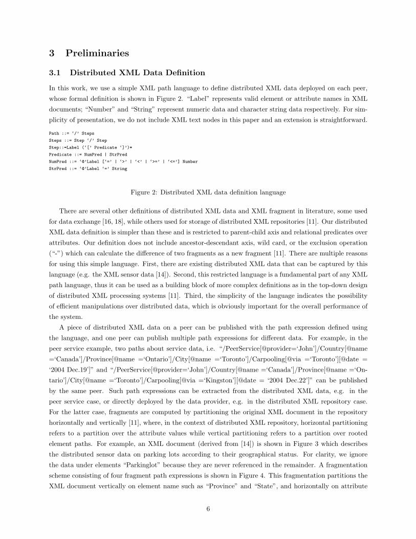
element paths. For example, an XML document (derived from [14]) is shown in Figure 3 which describes

the distributed sensor data on parking lots according to their geographical status. For clarity, we ignore

the data under elements “Parkinglot” because they are never referenced in the remainder. A fragmentation

scheme consisting of four fragment path expressions is shown in Figure 4. This fragmentation partitions the

XML document vertically on element name such as “Province” and “State”, and horizontally on attribute

6

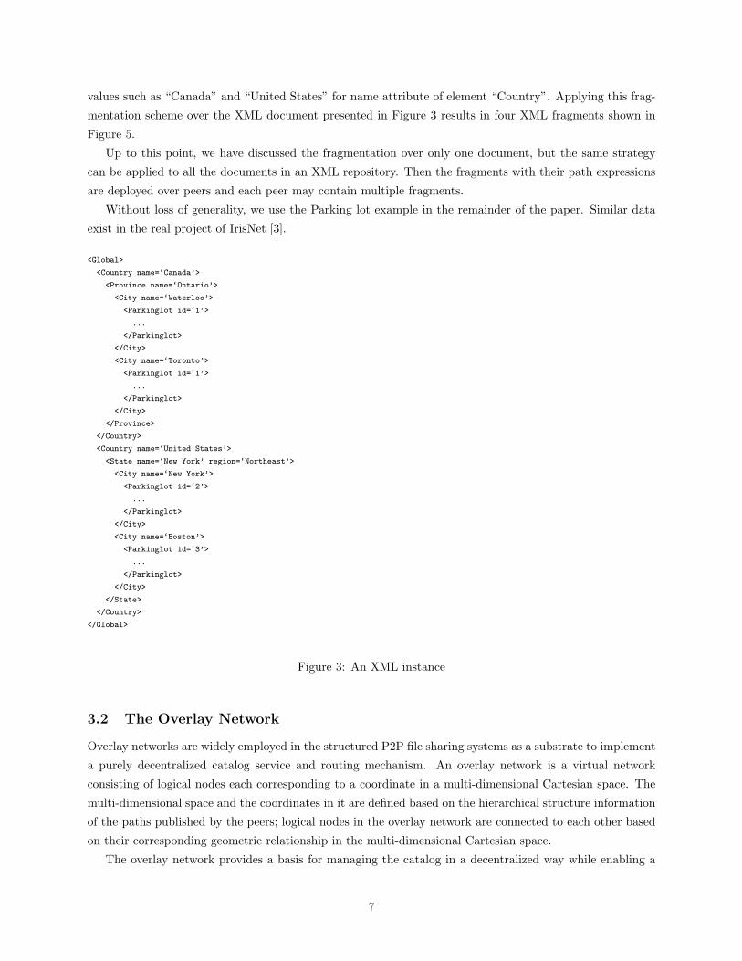
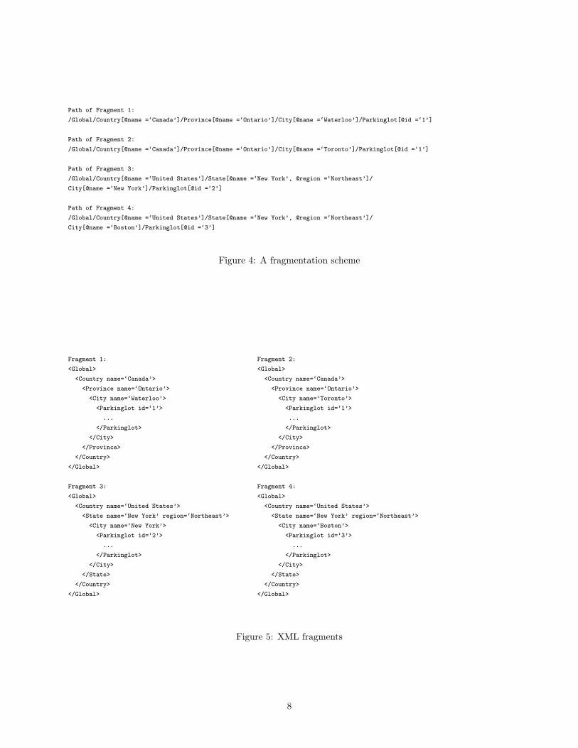
values such as “Canada” and “United States” for name attribute of element “Country”. Applying this frag-

mentation scheme over the XML document presented in Figure 3 results in four XML fragments shown in

Figure 5.

Up to this point, we have discussed the fragmentation over only one document, but the same strategy

can be applied to all the documents in an XML repository. Then the fragments with their path expressions

are deployed over peers and each peer may contain multiple fragments.

Without loss of generality, we use the Parking lot example in the remainder of the paper. Similar data

exist in the real project of IrisNet [3].

<Global>

<Country name=‘Canada’>

<Province name=‘Ontario’>

<City name=‘Waterloo’>

<Parkinglot id=‘1’>

...

</Parkinglot>

</City>

<City name=‘Toronto’>

<Parkinglot id=‘1’>

...

</Parkinglot>

</City>

</Province>

</Country>

<Country name=‘United States’>

<State name=‘New York’ region=‘Northeast’>

<City name=‘New York’>

<Parkinglot id=‘2’>

...

</Parkinglot>

</City>

<City name=‘Boston’>

<Parkinglot id=‘3’>

...

</Parkinglot>

</City>

</State>

</Country>

</Global>

Figure 3: An XML instance

3.2 The Overlay Network

Overlay networks are widely employed in the structured P2P file sharing systems as a substrate to implement

a purely decentralized catalog service and routing mechanism. An overlay network is a virtual network

consisting of logical nodes each corresponding to a coordinate in a multi-dimensional Cartesian space. The

multi-dimensional space and the coordinates in it are defined based on the hierarchical structure information

of the paths published by the peers; logical nodes in the overlay network are connected to each other based

on their corresponding geometric relationship in the multi-dimensional Cartesian space.

The overlay network provides a basis for managing the catalog in a decentralized way while enabling a

7

Path of Fragment 1:

/Global/Country[@name =‘Canada’]/Province[@name =‘Ontario’]/City[@name =‘Waterloo’]/Parkinglot[@id =‘1’]

Path of Fragment 2:

/Global/Country[@name =‘Canada’]/Province[@name =‘Ontario’]/City[@name =‘Toronto’]/Parkinglot[@id =‘1’]

Path of Fragment 3:

/Global/Country[@name =‘United States’]/State[@name =‘New York’, @region =‘Northeast’]/

City[@name =‘New York’]/Parkinglot[@id =‘2’]

Path of Fragment 4:

/Global/Country[@name =‘United States’]/State[@name =‘New York’, @region =‘Northeast’]/

City[@name =‘Boston’]/Parkinglot[@id =‘3’]

Figure 4: A fragmentation scheme

Fragment 1: Fragment 2:

<Global> <Global>

<Country name=‘Canada’> <Country name=‘Canada’>

<Province name=‘Ontario’> <Province name=‘Ontario’>

<City name=‘Waterloo’> <City name=‘Toronto’>

<Parkinglot id=‘1’> <Parkinglot id=‘1’>

... ...

</Parkinglot> </Parkinglot>

</City> </City>

</Province> </Province>

</Country> </Country>

</Global> </Global>

Fragment 3: Fragment 4:

<Global> <Global>

<Country name=‘United States’> <Country name=‘United States’>

<State name=‘New York’ region=‘Northeast’> <State name=‘New York’ region=‘Northeast’>

<City name=‘New York’> <City name=‘Boston’>

<Parkinglot id=‘2’> <Parkinglot id=‘3’>

... ...

</Parkinglot> </Parkinglot>

</City> </City>

</State> </State>

</Country> </Country>

</Global> </Global>

Figure 5: XML fragments

8

routing mechanism that locates the distributed XML data according to the hierarchial structure information,

rather than using the IP addresses as in IP routing. A number of proposals exist for catalog management and

routing: Chord [26], CAN [22], etc. Our approach is similar to CAN, but there are important differences.

CAN uses the Cartesian space to ensure the relationships among the nodes in the overlay network, but their

primary goal of using the cartesian space is for the even distribution of the data in the overlay network,

while our objective is to encode the hierarchical structure information of the distributed XML data in the

overlay network.

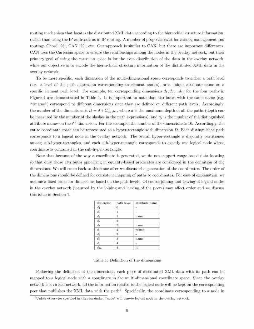
To be more specific, each dimension of the multi-dimensional space corresponds to either a path level

(i.e. a level of the path expression corresponding to element names), or a unique attribute name on a

specific element path level. For example, ten corresponding dimensions d1, d2, ...d10 for the four paths in

Figure 4 are demonstrated in Table 1. It is important to note that attributes with the same name (e.g.

“@name”) correspond to different dimensions since they are defined on different path levels. Accordingly,

the number of the dimensions is D = d + Σdi=1ai, where d is the maximum depth of all the paths (depth can

be measured by the number of the slashes in the path expressions), and ai is the number of the distinguished

attribute names on the ith dimension. For this example, the number of the dimensions is 10. Accordingly, the

entire coordinate space can be represented as a hyper-rectangle with dimension D. Each distinguished path

corresponds to a logical node in the overlay network. The overall hyper-rectangle is disjointly partitioned

among sub-hyper-rectangles, and each sub-hyper-rectangle corresponds to exactly one logical node whose

coordinate is contained in the sub-hyper-rectangle.

Note that because of the way a coordinate is generated, we do not support range-based data locating

so that only those attributes appearing in equality-based predicates are considered in the definition of the

dimensions. We will come back to this issue after we discuss the generation of the coordinates. The order of

the dimensions should be defined for consistent mapping of paths to coordinates. For ease of explanation, we

assume a fixed order for dimensions based on the path levels. Of course joining and leaving of logical nodes

in the overlay network (incurred by the joining and leaving of the peers) may affect order and we discuss

this issue in Section 7.

dimension path level attribute name

d1 0 -

d2 1 -

d3 1 name

d4 2 -

d5 2 name

d6 2 region

d7 3 -

d8 3 name

d9 4 -

d10 4 id

Table 1: Definition of the dimensions

Following the definition of the dimensions, each piece of distributed XML data with its path can be

mapped to a logical node with a coordinate in the multi-dimensional coordinate space. Since the overlay

network is a virtual network, all the information related to the logical node will be kept on the corresponding

peer that publishes the XML data with the path5. Specifically, the coordinate corresponding to a node in5Unless otherwise specified in the remainder, “node” will denote logical node in the overlay network.

9

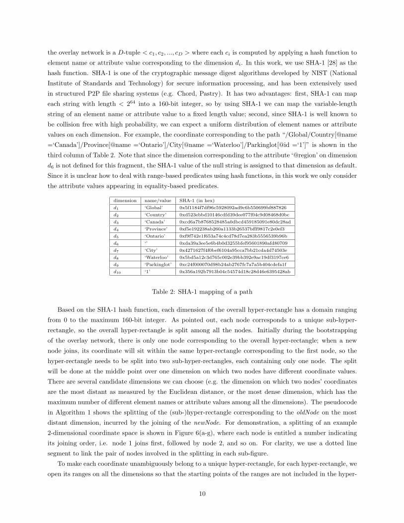
the overlay network is a D-tuple < c1, c2, ..., cD > where each ci is computed by applying a hash function to

element name or attribute value corresponding to the dimension di. In this work, we use SHA-1 [28] as the

hash function. SHA-1 is one of the cryptographic message digest algorithms developed by NIST (National

Institute of Standards and Technology) for secure information processing, and has been extensively used

in structured P2P file sharing systems (e.g. Chord, Pastry). It has two advantages: first, SHA-1 can map

each string with length < 264 into a 160-bit integer, so by using SHA-1 we can map the variable-length

string of an element name or attribute value to a fixed length value; second, since SHA-1 is well known to

be collision free with high probability, we can expect a uniform distribution of element names or attribute

values on each dimension. For example, the coordinate corresponding to the path “/Global/Country[@name

=‘Canada’]/Province[@name =‘Ontario’]/City[@name =‘Waterloo’]/Parkinglot[@id =‘1’]” is shown in the

third column of Table 2. Note that since the dimension corresponding to the attribute ‘@region’ on dimension

d6 is not defined for this fragment, the SHA-1 value of the null string is assigned to that dimension as default.

Since it is unclear how to deal with range-based predicates using hash functions, in this work we only consider

the attribute values appearing in equality-based predicates.

dimension name/value SHA-1 (in hex)

d1 ‘Global’ 0x5f1184f7df96c5928092ad9c6b550699bf887826

d2 ‘Country’ 0xd523ebbd10146cdfd39dee077f04c9d08468d0bc

d3 ‘Canada’ 0xcd6a7b8768528485a0dbcd459185091e80dc28ad

d4 ‘Province’ 0xf5e192238ab260a1133b26537bfff9817c2e0ef3

d5 ‘Ontario’ 0xf9f742e1f653a74c4cd78d7ea283b5556539b96b

d6 ‘’ 0xda39a3ee5e6b4b0d3255bfef95601890afd80709

d7 ‘City’ 0x4271627f4f0bef6104a95cca7bb21cda4d74503e

d8 ‘Waterloo’ 0x5bd5a12c3d765c002e39bb392e9ac19df3197ce6

d9 ‘Parkinglot’ 0xc24f000070d98b24ab2767fc7a7a5b404cdefa1f

d10 ‘1’ 0x356a192b7913b04c54574d18c28d46e6395428ab

Table 2: SHA-1 mapping of a path

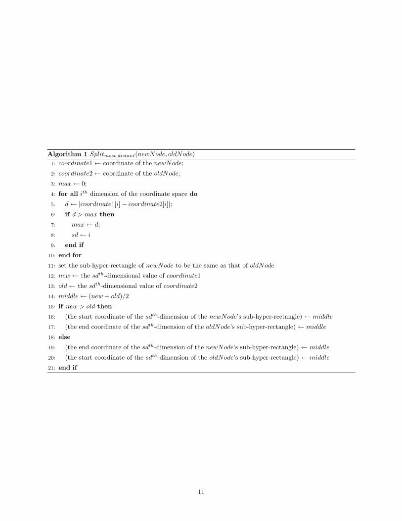
Based on the SHA-1 hash function, each dimension of the overall hyper-rectangle has a domain ranging

from 0 to the maximum 160-bit integer. As pointed out, each node corresponds to a unique sub-hyper-

rectangle, so the overall hyper-rectangle is split among all the nodes. Initially during the bootstrapping

of the overlay network, there is only one node corresponding to the overall hyper-rectangle; when a new

node joins, its coordinate will sit within the same hyper-rectangle corresponding to the first node, so the

hyper-rectangle needs to be split into two sub-hyper-rectangles, each containing only one node. The split

will be done at the middle point over one dimension on which two nodes have different coordinate values.

There are several candidate dimensions we can choose (e.g. the dimension on which two nodes’ coordinates

are the most distant as measured by the Euclidean distance, or the most dense dimension, which has the

maximum number of different element names or attribute values among all the dimensions). The pseudocode

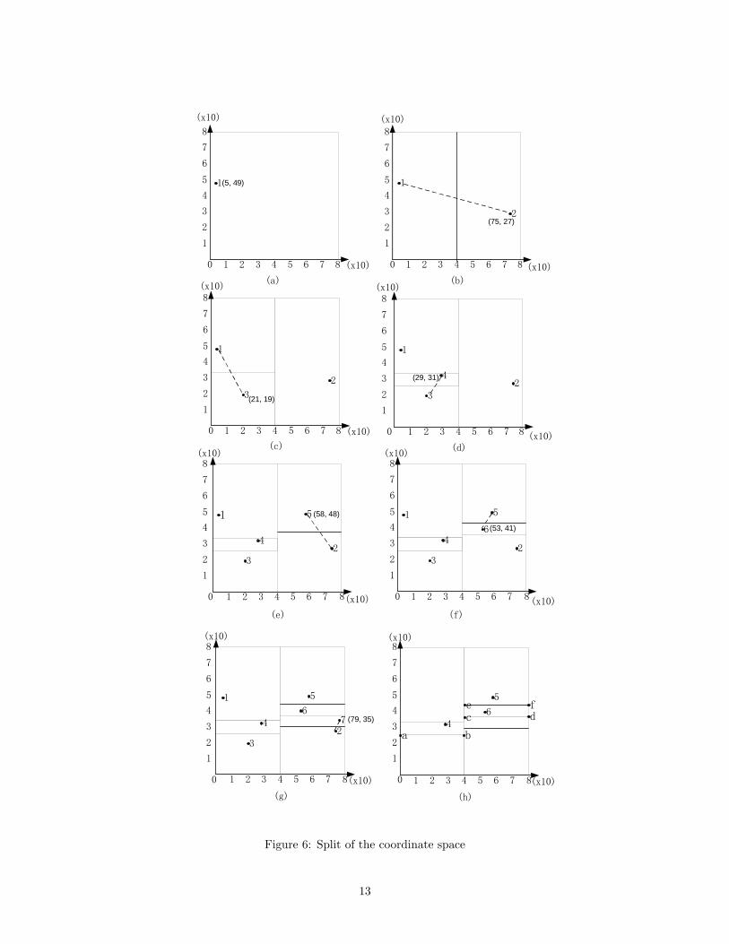
in Algorithm 1 shows the splitting of the (sub-)hyper-rectangle corresponding to the oldNode on the most

distant dimension, incurred by the joining of the newNode. For demonstration, a splitting of an example

2-dimensional coordinate space is shown in Figure 6(a-g), where each node is entitled a number indicating

its joining order, i.e. node 1 joins first, followed by node 2, and so on. For clarity, we use a dotted line

segment to link the pair of nodes involved in the splitting in each sub-figure.

To make each coordinate unambiguously belong to a unique hyper-rectangle, for each hyper-rectangle, we

open its ranges on all the dimensions so that the starting points of the ranges are not included in the hyper-

10

Algorithm 1 Splitmost distant(newNode, oldNode)1: coordinate1← coordinate of the newNode;

2: coordinate2← coordinate of the oldNode;

3: max← 0;

4: for all ith dimension of the coordinate space do

5: d← |coordinate1[i]− coordinate2[i]|;6: if d > max then

7: max← d;

8: sd← i

9: end if

10: end for

11: set the sub-hyper-rectangle of newNode to be the same as that of oldNode

12: new ← the sdth-dimensional value of coordinate1

13: old← the sdth-dimensional value of coordinate2

14: middle← (new + old)/2

15: if new > old then

16: (the start coordinate of the sdth-dimension of the newNode’s sub-hyper-rectangle) ← middle

17: (the end coordinate of the sdth-dimension of the oldNode’s sub-hyper-rectangle) ← middle

18: else

19: (the end coordinate of the sdth-dimension of the newNode’s sub-hyper-rectangle) ← middle

20: (the start coordinate of the sdth-dimension of the oldNode’s sub-hyper-rectangle) ← middle

21: end if

11

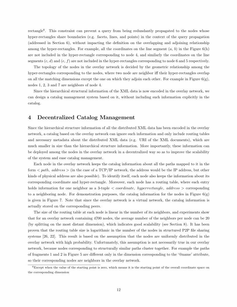
rectangle6. This constraint can prevent a query from being redundantly propagated to the nodes whose

hyper-rectangles share boundaries (e.g. facets, lines, and points) in the context of the query propagation

(addressed in Section 6), without impacting the definition on the overlapping and adjoining relationship

among the hyper-rectangles. For example, all the coordinates on the line segment (a, b) in the Figure 6(h)

are not included in the hyper-rectangle corresponding to node 4, and similarly the coordinates on the line

segments (c, d) and (e, f) are not included in the hyper-rectangles corresponding to node 6 and 5 respectively.

The topology of the nodes in the overlay network is decided by the geometric relationship among the

hyper-rectangles corresponding to the nodes, where two node are neighbor iff their hyper-rectangles overlap

on all the matching dimensions except the one on which they adjoin each other. For example in Figure 6(g),

nodes 1, 2, 3 and 7 are neighbors of node 4.

Since the hierarchical structural information of the XML data is now encoded in the overlay network, we

can design a catalog management system based on it, without including such information explicitly in the

catalog.

4 Decentralized Catalog Management

Since the hierarchical structure information of all the distributed XML data has been encoded in the overlay

network, a catalog based on the overlay network can ignore such information and only include routing tables

and necessary metadata about the distributed XML data (e.g. URI of the XML documents), which are

much smaller in size than the hierarchical structure information. More importantly, these information can

be deployed among the nodes in the overlay network in a decentralized way so as to improve the scalability

of the system and ease catalog management.

Each node in the overlay network keeps the catalog information about all the paths mapped to it in the

form < path, address > (in the case of a TCP/IP network, the address would be the IP address, but other

kinds of physical address are also possible). To identify itself, each node also keeps the information about its

corresponding coordinate and hyper-rectangle. Moreover, each node has a routing table, where each entry

holds information for one neighbor as a 3-tuple < coordinate, hyperrectangle, address > corresponding

to a neighboring node. For demonstration purposes, the catalog information for the nodes in Figure 6(g)

is given in Figure 7. Note that since the overlay network is a virtual network, the catalog information is

actually stored on the corresponding peers.

The size of the routing table at each node is linear in the number of its neighbors, and experiments show

that for an overlay network containing 4700 nodes, the average number of the neighbors per node can be 20

(by splitting on the most distant dimension), which indicates good scalability (see Section 8). It has been

proven that the routing table size is logarithmic in the number of the nodes in structured P2P file sharing

systems [26, 22]. This result is based on the assumption that the nodes are uniformly distributed in the

overlay network with high probability. Unfortunately, this assumption is not necessarily true in our overlay

network, because nodes corresponding to structurally similar paths cluster together. For example the paths

of fragments 1 and 2 in Figure 5 are different only in the dimension corresponding to the ‘@name’ attribute,

so their corresponding nodes are neighbors in the overlay network.6Except when the value of the starting point is zero, which means it is the starting point of the overall coordinate space on

the corresponding dimension

12

0

1

2

3

4

5

6

7

8

(x10)

(x10)

0 1 2 3 4 5 6 7

1

2

3

4

5

6

7

8

1

2

8

(b)

(x10)

(x10)

(x10)

0 1 2 3 4 5 6 7

1

2

3

4

5

6

7

8

1

8

(a)

(5, 49)

(75, 27)

0

1

2

3

4

5

6

7

8

1 2 3 4 5 6 7

1

3

42

0 1 2 3 4 5 6 7

1

2

3

4

5

6

7

8

1

3

2

8

(c) (d)

8(x10) (x10)

(x10)

(29, 31)

(21, 19)

(x10)

(x10)

8 01 2 3 4 5 6 7

1

2

3

4

5

6

7

8

1

3

42

5

67

(g)

(x10)

(79, 35)

(x10)

81 2 3 4 5 6 7

4

5

6

(h)

b

ec

0

1

2

3

4

5

6

7

8

1 2 3 4 5 6 7

1

3

42

5

80 1 2 3 4 5 6 7

1

2

3

4

5

6

7

8

1

3

42

6

8

(e) (f)

(x10)

(x10)

(x10)

(58, 48)

(53, 41)

5

(x10)

(x10)

a

df

Figure 6: Split of the coordinate space

13

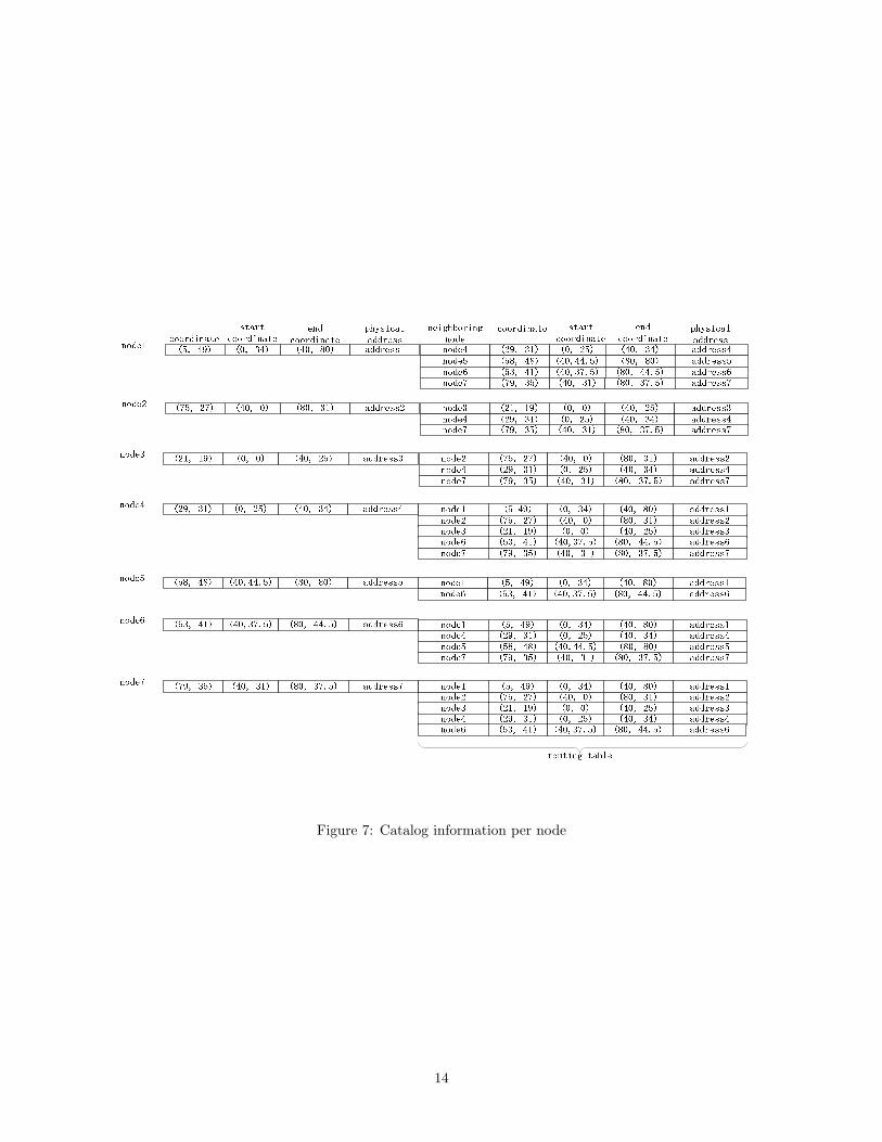
Figure 7: Catalog information per node

14

Catalog also includes metadata about the distributed XML data deployed in the P2P network. For ex-

ample, in the distributed XML repository case, URI (Universal Resource Identifier) information is important

to distinguish different XML documents deployed over the same P2P network. We replicate the metadata on

each node by reserving for it a special dimension in the multi-dimensional coordinate space. Furthermore,

as pointed out, the XML schema information used to execute queries is available on peers, which is useful

for query rewriting. Since each peer only needs to know the schema in which it is interested, such metadata

can be regarded as partially replicated in the network. Other useful metadata include the number of distin-

guished element names or attribute values on each dimension defined in the overlay network, which can be

used in the splitting algorithm shown in Algorithm 1 (e.g. when choosing the dimension with the maximum

number of different element names). This global statistical information can be deployed on a specific logical

node (physically on the corresponding peer) whose corresponding hyper-rectangle covers the coordinate of

(0, 0, 0, ...0). However, for better scalability, we replicate the information on several nodes in the overlay

network, e.g. the node whose corresponding hyper-rectangle covers the coordinate of (xi, 0, 0, ...0), where

xi is the SHA-1 hash value of the URI corresponding to each different XML document in the distributed

XML repository case. The problem of employing this information is that if peers join and leave the network

very frequently, the maintenance cost will be high. Fortunately, the experiments show that the splitting

algorithm based on the most distant dimension shows good scalability over thousands of nodes, so that we

can choose this option to keep the catalog management in a purely decentralized manner.

Since the URI information and the schema information can be expected to be stable, little maintenance

is needed. Then the biggest catalog maintenance work is on the routing tables: changes on the topology of

the overlay network affect the routing tables of the related nodes. For example, if a node leaves the overlay

network, its corresponding entries in its neighbors’ routing tables need to be removed and new entries are then

created there based on the new neighboring relationships among the remaining nodes. Since the maintenance

work is distributed among all the peers, we can expect the catalog management to be scalable over large-scale

P2P networks.

5 Routing towards peers

In the environment that is considered, XML data is distributed and stored on peers, as described above,

where the data is defined by paths. A fundamental point of query processing in this environment is to

efficiently match data to queries without extensive communication overhead. In this section we discuss a

multi-hop routing algorithm to reach an arbitrary peer. This algorithm is the basis of the data locating

mechanism described in the next section.

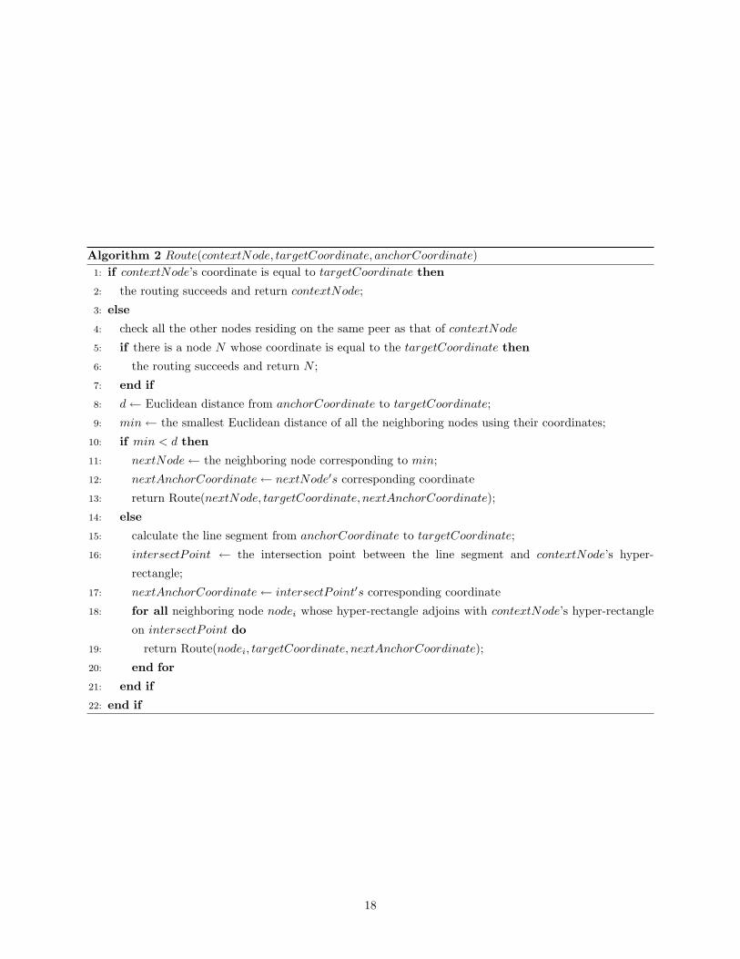
The routing algorithm is given in Algorithm 2, which works as follows. The target peer has a target

node in the overlay network and we call its corresponding coordinate as target coordinate; during each hop,

a node is reached that we call the context node. When a context node is reached (including the initial

node), its coordinate is checked against the target coordinate. If the target node is not reached, the context

node’s routing table is scanned and the neighboring node whose hyper-rectangle is geometrically closest

to the target coordinate is chosen as the context node for the next hop. The process continues until the

target is reached. Remember that a peer may publish multiple pieces of XML data resulting in multiple

overlay network nodes corresponding to that peer. So it is possible that the context node shares the same

peer as that corresponding to the target coordinate. To exploit this, in each hop all the other logical nodes

15

deployed on the peer corresponding to the context node are matched against the target coordinate for an

early finding. This is reflected in lines 4 and 5 of Algorithm 2. Furthermore, by replacing the equality tests

in lines 1 and 5 of the Algorithm 2 with containment tests to check whether targetCoordinate is contained

in the hyper-rectangles corresponding to contextNode and N respectively, the algorithm can route towards

any peer corresponding to the nodes whose hyper-rectangle cover specific coordinates such as (xi, 0, 0, ...0)

and (0, 0, 0, ...0), as used by the catalog management mentioned in the previous section.

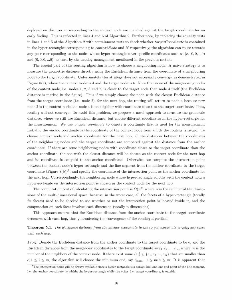
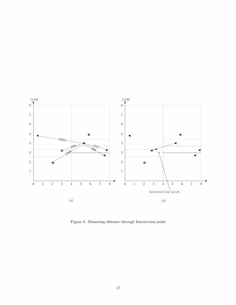
The crucial part of this routing algorithm is how to choose a neighboring node. A naive strategy is to

measure the geometric distance directly using the Euclidean distance from the coordinate of a neighboring

node to the target coordinate. Unfortunately this strategy does not necessarily converge, as demonstrated in

Figure 8(a), where the context node is 4 and the target node is 6. Note that none of the neighboring nodes

of the context node, i.e. nodes 1, 2, 3 and 7, is closer to the target node than node 4 itself (the Euclidean

distance is marked in the figure). Thus if we simply choose the node with the closest Euclidean distance

from the target coordinate (i.e. node 2), for the next hop, the routing will return to node 4 because now

node 2 is the context node and node 4 is its neighbor with coordinate closest to the target coordinate. Thus,

routing will not converge. To avoid this problem, we propose a novel approach to measure the geometric

distance, where we still use Euclidean distance, but choose different coordinates in the hyper-rectangle for

the measurement. We use anchor coordinate to denote a coordinate that is used for the measurement.

Initially, the anchor coordinate is the coordinate of the context node from which the routing is issued. To

choose context node and anchor coordinate for the next hop, all the distances between the coordinates

of the neighboring nodes and the target coordinate are compared against the distance from the anchor

coordinate. If there are some neighboring nodes with coordinate closer to the target coordinate than the

anchor coordinate, the one with the closest distance will be chosen as the context node for the next hop

and its coordinate is assigned to the anchor coordinate. Otherwise, we compute the intersection point

between the context node’s hyper-rectangle and the line segment from the anchor coordinate to the target

coordinate (Figure 8(b))7, and specify the coordinate of the intersection point as the anchor coordinate for

the next hop. Correspondingly, the neighboring node whose hyper-rectangle adjoins with the context node’s

hyper-rectangle on the intersection point is chosen as the context node for the next hop.

The computation cost of calculating the intersection point is O(n2) where n is the number of the dimen-

sions of the multi-dimensional space, because, in the worst case, all the facets of a hyper-rectangle (totally

2n facets) need to be checked to see whether or not the intersection point is located inside it, and the

computation on each facet involves each dimension (totally n dimensions).

This approach ensures that the Euclidean distance from the anchor coordinate to the target coordinate

decreases with each hop, thus guaranteeing the convergence of the routing algorithm.

Theorem 5.1. The Euclidean distance from the anchor coordinate to the target coordinate strictly decreases

with each hop.

Proof. Denote the Euclidean distance from the anchor coordinate to the target coordinate to be e, and the

Euclidean distances from the neighbors’ coordinates to the target coordinate as e1, e2, ..., em, where m is the

number of the neighbors of the context node. If there exist some {ei} ⊆ {e1, e2, ..., em} that are smaller than

e, 1 ≤ i ≤ m, the algorithm will choose the minimum one, say emin, 1 ≤ min ≤ m. It is apparent that7The intersection point will be always available since a hyper-rectangle is a convex hull and one end point of the line segment,

i.e. the anchor coordinate, is within the hyper-rectangle while the other, i.e. target coordinate, is outside.

16

80 1 2 3 4 5 6 7

1

2

3

4

5

6

7

8

1

3

4

2

5

6

7

(x10)

676

1508

2353

680712

80 1 2 3 4 5 6 7

1

2

3

4

5

6

7

8

1

3

4

2

5

6

7

(x10)

Intersection point

(a) (b)

Figure 8: Measuring distance through Intersection point

17

Algorithm 2 Route(contextNode, targetCoordinate, anchorCoordinate)1: if contextNode’s coordinate is equal to targetCoordinate then

2: the routing succeeds and return contextNode;

3: else

4: check all the other nodes residing on the same peer as that of contextNode

5: if there is a node N whose coordinate is equal to the targetCoordinate then

6: the routing succeeds and return N ;

7: end if

8: d← Euclidean distance from anchorCoordinate to targetCoordinate;

9: min← the smallest Euclidean distance of all the neighboring nodes using their coordinates;

10: if min < d then

11: nextNode← the neighboring node corresponding to min;

12: nextAnchorCoordinate← nextNode′s corresponding coordinate

13: return Route(nextNode, targetCoordinate, nextAnchorCoordinate);

14: else

15: calculate the line segment from anchorCoordinate to targetCoordinate;

16: intersectPoint ← the intersection point between the line segment and contextNode’s hyper-

rectangle;

17: nextAnchorCoordinate← intersectPoint′s corresponding coordinate

18: for all neighboring node nodei whose hyper-rectangle adjoins with contextNode’s hyper-rectangle

on intersectPoint do

19: return Route(nodei, targetCoordinate, nextAnchorCoordinate);

20: end for

21: end if

22: end if

18

emin is strictly smaller than the Euclidean distance from the coordinate of the context node to the target

coordinate. On the other hand, if no ei ∈ {e1, e2, ..., em} is smaller than e, the anchor coordinate of the next

hop will be the intersection point’s coordinate, which indicates a strictly smaller Euclidean distance because

the intersection point is located on the line segment between the two end points, i.e. the anchor coordinate

and the target coordinate.

Our routing algorithm differs from that in the CAN system [22] in the strategy we use to find a neighboring

node for the next hop. The measurement of the geometric distance directly using the coordinate of the context

node, as done in CAN, works only if the coordinate space is evenly split among all the nodes so that, with

high probability, there exist some neighboring nodes with coordinates closer to the target coordinate. This

is not true in general and does not hold in our case, since nodes corresponding to structurally similar paths

(and also data) cluster in the coordinate space. Sahin et al. develop a strategy on choosing the closest

neighboring node [25], where the geometric distance from the context node’s hyper-rectangle to the target

coordinate is measured from the facet adjoining with a neighboring zone of the context node which covers

the target coordinate. The computation cost is the same but the strategy is quite different.

6 Locating Relevant Data for Complex Queries

Based on the decentralized catalog management and routing mechanism described in the previous section,

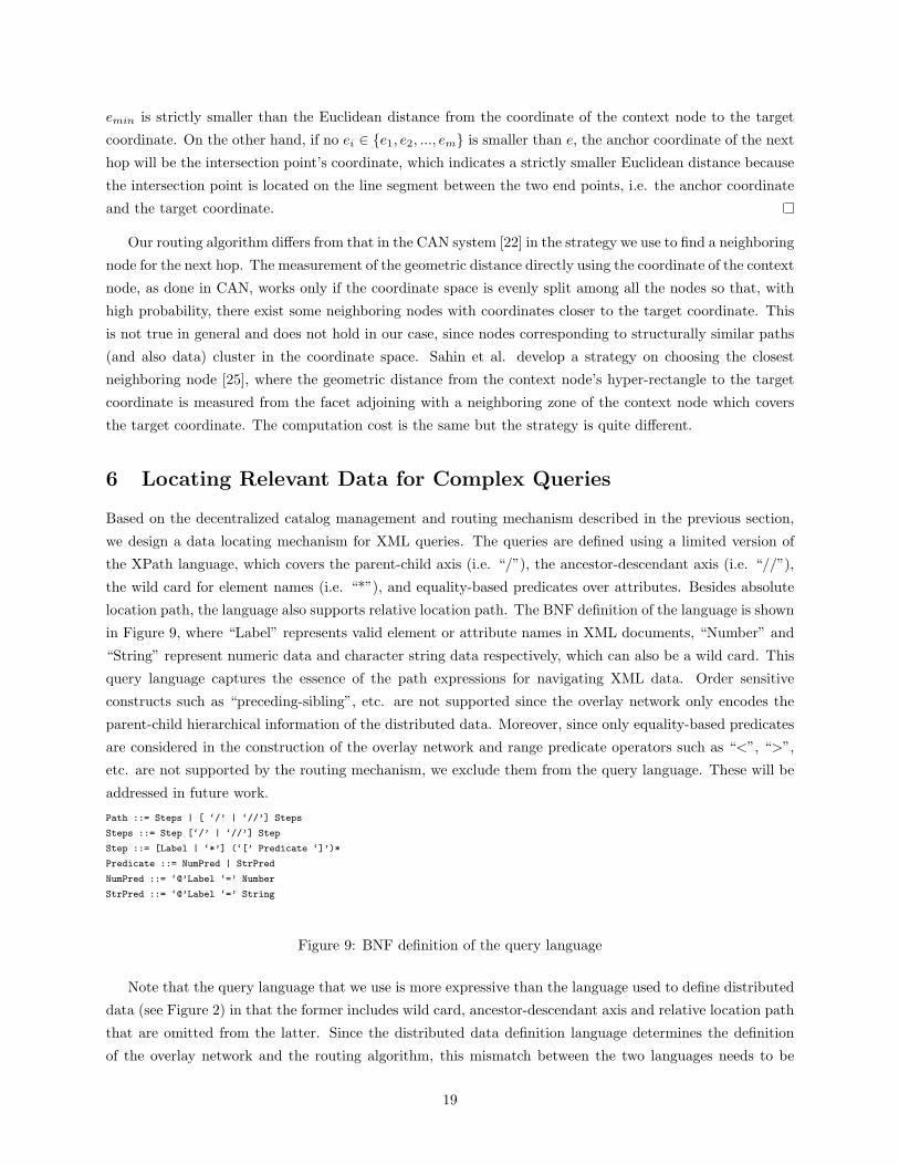
we design a data locating mechanism for XML queries. The queries are defined using a limited version of

the XPath language, which covers the parent-child axis (i.e. “/”), the ancestor-descendant axis (i.e. “//”),

the wild card for element names (i.e. “*”), and equality-based predicates over attributes. Besides absolute

location path, the language also supports relative location path. The BNF definition of the language is shown

in Figure 9, where “Label” represents valid element or attribute names in XML documents, “Number” and

“String” represent numeric data and character string data respectively, which can also be a wild card. This

query language captures the essence of the path expressions for navigating XML data. Order sensitive

constructs such as “preceding-sibling”, etc. are not supported since the overlay network only encodes the

parent-child hierarchical information of the distributed data. Moreover, since only equality-based predicates

are considered in the construction of the overlay network and range predicate operators such as “<”, “>”,

etc. are not supported by the routing mechanism, we exclude them from the query language. These will be

addressed in future work.

Path ::= Steps | [ ‘/’ | ‘//’] Steps

Steps ::= Step [‘/’ | ‘//’] Step

Step ::= [Label | ‘*’] (‘[’ Predicate ‘]’)*

Predicate ::= NumPred | StrPred

NumPred ::= ‘@’Label ‘=’ Number

StrPred ::= ‘@’Label ‘=’ String

Figure 9: BNF definition of the query language

Note that the query language that we use is more expressive than the language used to define distributed

data (see Figure 2) in that the former includes wild card, ancestor-descendant axis and relative location path

that are omitted from the latter. Since the distributed data definition language determines the definition

of the overlay network and the routing algorithm, this mismatch between the two languages needs to be

19

addressed. Briefly, the data locating for a query is transformed into a routing process towards a peer if

the following two conditions are satisfied: (1) the query contains only absolute location path and parent-

child axis, and (2) the query is defined on all the dimensions of the overlay network. Otherwise, for queries

containing wild card or ancestor-descendant axis, and queries that are not fully defined on all the dimensions,

the data locating mechanism will first locate a rendezvous node which is related to the query from where

the query is propagated in a limited subnetwork. Since there is no centralized catalog providing a complete

mapping of a query to candidate paths published in the network, a propagation is unavoidable. By choosing

a rendezvous node first and then making a limited broadcast, we avoid the naive flooding utilized in some

P2P file sharing systems. The experiments show good scalability of our data locating mechanism for all

kinds of queries.

6.1 Queries with absolute location path and parent-child axis

As mentioned above, queries that only contain absolute location path and parent-child axis completely match

the distributed XML data definition language. Thus the query path expression can be hashed to a coordinate

in the same way as a path published by peers in the network. We call this the query coordinate.

If the path expression of a query is defined on all the dimensions of the coordinate space, locating the

relevant data can be accomplished by routing the query towards the peer that publishes the same path. For

example, a query can be“/Global/Country[@name =‘United States’]/State[@name =‘New York’][@region

=‘Northeast’]/City[@name =‘New York’]/Parkinglot[@id =‘2’]”, which satisfies the above conditions. Thus

the relevant data can be located by directly routing the query towards the corresponding query coordinate

in the overlay network.

A more complicated case is that some dimensions are not defined in the query. For these missing

dimensions, we assign SHA-1 hash value of the null string as default values, denoted as “#” for con-

venience. For example, based on the dimensions defined in Table 1, the query coordinate of the query

“/Global/Country[@name =‘Canada’]/Province[@name =‘Ontario’]/City” is shown in the third column of

Table 3, which has four default values corresponding to the missing dimensions (i.e. Province region, City

name, Parkinglot, and Parkinglot id). Such a query can not be rewritten into paths published in the P2P

network without a centralized catalog. We solve this problem by propagating the query within a limited part

of the overlay network. In principle, all the nodes in the overlay network matching the query should be cov-

ered by a sub-coordinate-space that is defined by the query coordinate. Specifically, on the dimensions that

the query is defined, the sub-coordinate-space takes the point values of the query coordinate as its ranges

(i.e. range with single value); otherwise on the dimensions that the query is not defined, the sub-coordinate-

space takes the full range of the overall coordinate space (i.e. 0 to the maximum of 160-bit integer). For

demonstration, the sub-coordinate-space corresponding to the query coordinate in the third column of Table

3 is shown in the fourth column. Note that we set the range corresponding to the missing dimensions to be

the whole domain of the dimension so as to cover all the possible values on it. There are still two problems:

(1) how to choose a starting point for the propagation, and (2) how to propagate the query so that all the

relevant logical nodes are exhausted. The answer to the first question is that we can start from any node

in the overlay network whose hyper-rectangle intersects with the sub-coordinate-space. The answer to the

second question is that we can propagate the query to all of its neighbors in the overlay network whose

hyper-rectangles intersect with the sub-coordinate-space. Here, the intersection between a hyper-rectangle

20

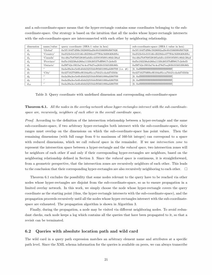
and a sub-coordinate-space means that the hyper-rectangle contains some coordinates belonging to the sub-

coordinate-space. Our strategy is based on the intuition that all the nodes whose hyper-rectangle intersects

with the sub-coordinate-space are interconnected with each other by neighboring relationship.

dimension name/value query coordinate (SHA-1 value in hex) sub-coordinate-space (SHA-1 value in hex)

d1 ‘Global’ 0x5f1184f7df96c5928092ad9c6b550699bf887826 0x5f1184f7df96c5928092ad9c6b550699bf887826

d2 ‘Country’ 0xd523ebbd10146cdfd39dee077f04c9d08468d0bc 0xd523ebbd10146cdfd39dee077f04c9d08468d0bc

d3 ‘Canada’ 0xcd6a7b8768528485a0dbcd459185091e80dc28ad 0xcd6a7b8768528485a0dbcd459185091e80dc28ad

d4 ‘Province’ 0xf5e192238ab260a1133b26537bfff9817c2e0ef3 0xf5e192238ab260a1133b26537bfff9817c2e0ef3

d5 ‘Ontario’ 0xf9f742e1f653a74c4cd78d7ea283b5556539b96b 0xf9f742e1f653a74c4cd78d7ea283b5556539b96b

d6 ‘’ 0xda39a3ee5e6b4b0d3255bfef95601890afd80709 (i.e. #) [0, 0xffffffffffffffffffffffffffffffffffffffff]

d7 ‘City’ 0x4271627f4f0bef6104a95cca7bb21cda4d74503e 0x4271627f4f0bef6104a95cca7bb21cda4d74503e

d8 ‘’ 0xda39a3ee5e6b4b0d3255bfef95601890afd80709 [0, 0xffffffffffffffffffffffffffffffffffffffff]

d9 ‘’ 0xda39a3ee5e6b4b0d3255bfef95601890afd80709 [0, 0xffffffffffffffffffffffffffffffffffffffff]

d10 ‘’ 0xda39a3ee5e6b4b0d3255bfef95601890afd80709 [0, 0xffffffffffffffffffffffffffffffffffffffff]

Table 3: Query coordinate with undefined dimension and corresponding sub-coordinate-space

Theorem 6.1. All the nodes in the overlay network whose hyper-rectangles intersect with the sub-coordinate-

space are, recursively, neighbors of each other in the overall coordinate space.

Proof. According to the definition of the intersection relationship between a hyper-rectangle and the same

sub-coordinate-space, if two arbitrary hyper-rectangles both intersect with the sub-coordinate-space, their

ranges must overlap on the dimensions on which the sub-coordinate-space has point values. Then the

remaining dimensions (with full range from 0 to maximum of 160-bit integer) can correspond to a space

with reduced dimensions, which we call reduced space in the remainder. If we use intersection zone to

represent the intersection space between a hyper-rectangle and the reduced space, two intersection zones will

be neighbors of each other if and only if their corresponding hyper-rectangles are neighbors, based on the

neighboring relationship defined in Section 3. Since the reduced space is continuous, it is straightforward,

from a geometric perspective, that the intersection zones are recursively neighbors of each other. This leads

to the conclusion that their corresponding hyper-rectangles are also recursively neighboring to each other.

Theorem 6.1 excludes the possibility that some nodes relevant to the query have to be reached via other

nodes whose hyper-rectangles are disjoint from the sub-coordinate-space, so as to ensure propagation in a

limited overlay network. In this work, we simply choose the node whose hyper-rectangle covers the query

coordinate as the starting point (thus, the hyper-rectangle intersects with the sub-coordinate-space), and the

propagation proceeds recursively until all the nodes whose hyper-rectangles intersect with the sub-coordinate-

space are exhausted. The propagation algorithm is shown in Algorithm 3.

Finally, during the propagation, a node may be visited via different neighboring nodes. To avoid redun-

dant checks, each node keeps a log which contains all the queries that have been propagated to it, so that a

revisit can be terminated.

6.2 Queries with absolute location path and wild card

The wild card in a query path expression matches an arbitrary element name and attributes at a specific

path level. Since the XML schema information for the queries is available on peers, we can always transcribe

21

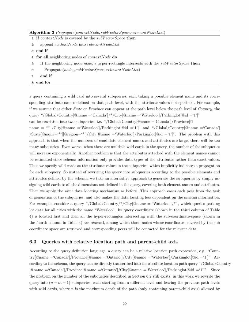
Algorithm 3 Propagate(contextNode, subV ectorSpace, relevantNodeList)1: if contextNode is covered by the subV ectorSpace then

2: append contextNode into relevantNodeList

3: end if

4: for all neighboring nodes of contextNode do

5: if the neighboring node nodei’s hyper-rectangle intersects with the subV ectorSpace then

6: Propagate(nodei, subV ectorSpace, relevantNodeList)

7: end if

8: end for

a query containing a wild card into several subqueries, each taking a possible element name and its corre-

sponding attribute names defined on that path level, with the attribute values not specified. For example,

if we assume that either State or Province can appear at the path level below the path level of Country, the

query “/Global/Country[@name =‘Canada’]/*/City[@name =‘Waterloo’]/Parkinglot[@id =‘1’]”

can be rewritten into two subqueries, i.e. “/Global/Country[@name =‘Canada’]/Province[@

name = ‘*’]/City[@name =‘Waterloo’]/Parkinglot[@id =‘1’]” and “/Global/Country[@name =‘Canada’]

/State[@name=‘*’][@region=‘*’]/City[@name =‘Waterloo’]/Parkinglot[@id =‘1’]”. The problem with this

approach is that when the numbers of candidate element names and attributes are large, there will be too

many subqueries. Even worse, when there are multiple wild cards in the query, the number of the subqueries

will increase exponentially. Another problem is that the attributes attached with the element names cannot

be estimated since schema information only provides data types of the attributes rather than exact values.

Thus we specify wild cards as the attribute values in the subqueries, which implicitly indicates a propagation

for each subquery. So instead of rewriting the query into subqueries according to the possible elements and

attributes defined by the schema, we take an alternative approach to generate the subqueries by simply as-

signing wild cards to all the dimensions not defined in the query, covering both element names and attributes.

Then we apply the same data locating mechanism as before. This approach eases each peer from the task

of generation of the subqueries, and also makes the data locating less dependent on the schema information.

For example, consider a query “/Global/Country/*/City[@name = ‘Waterloo’]/*”, which queries parking

lot data for all cities with the name “Waterloo”. Its query coordinate (shown in the third column of Table

4) is located first and then all the hyper-rectangles intersecting with the sub-coordinate-space (shown in

the fourth column in Table 4) are reached, among which those nodes whose coordinates covered by the sub

coordinate space are retrieved and corresponding peers will be contacted for the relevant data.

6.3 Queries with relative location path and parent-child axis

According to the query definition language, a query can be a relative location path expression, e.g. “Coun-

try[@name =‘Canada’]/Province[@name =‘Ontario’]/City[@name =‘Waterloo’]/Parkinglot[@id =‘1’]”. Ac-

cording to the schema, the query can be directly transcribed into the absolute location path query “/Global/Country

[@name =‘Canada’]/Province[@name =‘Ontario’]/City[@name =‘Waterloo’]/Parkinglot[@id =‘1’]”. Since

the problem on the number of the subqueries described in Section 6.2 still exists, in this work we rewrite the

query into (n −m + 1) subqueries, each starting from a different level and leaving the previous path levels

with wild cards, where n is the maximum depth of the path (only containing parent-child axis) allowed by

22

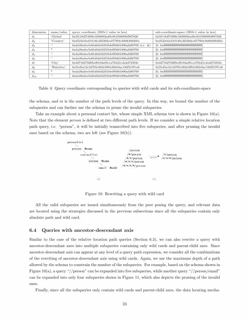
dimension name/value query coordinate (SHA-1 value in hex) sub-coordinate-space (SHA-1 value in hex)

d1 ‘Global’ 0x5f1184f7df96c5928092ad9c6b550699bf887826 0x5f1184f7df96c5928092ad9c6b550699bf887826

d2 ‘Country’ 0xd523ebbd10146cdfd39dee077f04c9d08468d0bc 0xd523ebbd10146cdfd39dee077f04c9d08468d0bc

d3 ‘’ 0xda39a3ee5e6b4b0d3255bfef95601890afd80709 (i.e. #) [0, 0xffffffffffffffffffffffffffffffffffffffff]

d4 * 0xda39a3ee5e6b4b0d3255bfef95601890afd80709 [0, 0xffffffffffffffffffffffffffffffffffffffff]

d5 ‘’ 0xda39a3ee5e6b4b0d3255bfef95601890afd80709 [0, 0xffffffffffffffffffffffffffffffffffffffff]

d6 ‘’ 0xda39a3ee5e6b4b0d3255bfef95601890afd80709 [0, 0xffffffffffffffffffffffffffffffffffffffff]

d7 ‘City’ 0x4271627f4f0bef6104a95cca7bb21cda4d74503e 0x4271627f4f0bef6104a95cca7bb21cda4d74503e

d8 ‘Waterloo’ 0x5bd5a12c3d765c002e39bb392e9ac19df3197ce6 0x5bd5a12c3d765c002e39bb392e9ac19df3197ce6

d9 * 0xda39a3ee5e6b4b0d3255bfef95601890afd80709 [0, 0xffffffffffffffffffffffffffffffffffffffff]

d10 ‘’ 0xda39a3ee5e6b4b0d3255bfef95601890afd80709 [0, 0xffffffffffffffffffffffffffffffffffffffff]

Table 4: Query coordinate corresponding to queries with wild cards and its sub-coordinate-space

the schema, and m is the number of the path levels of the query. In this way, we bound the number of the

subqueries and can further use the schema to prune the invalid subqueries.

Take an example about a personal contact list, whose simple XML schema tree is shown in Figure 10(a).

Note that the element person is defined at two different path levels. If we consider a simple relative location

path query, i.e. “person”, it will be initially transcribed into five subqueries, and after pruning the invalid

ones based on the schema, two are left (see Figure 10(b)).

Figure 10: Rewriting a query with wild card

All the valid subqueries are issued simultaneously from the peer posing the query, and relevant data

are located using the strategies discussed in the previous subsections since all the subqueries contain only

absolute path and wild card.

6.4 Queries with ancestor-descendant axis

Similar to the case of the relative location path queries (Section 6.3), we can also rewrite a query with

ancestor-descendant axes into multiple subqueries containing only wild cards and parent-child axes. Since

ancestor-descendant axis can appear at any level of a query path expression, we consider all the combinations

of the rewriting of ancestor-descendant axis using wild cards. Again, we use the maximum depth of a path

allowed by the schema to constrain the number of the subqueries. For example, based on the schema shown in

Figure 10(a), a query “//person” can be expanded into five subqueries, while another query “//person/email”

can be expanded into only four subqueries shown in Figure 11, which also depicts the pruning of the invalid

ones.

Finally, since all the subqueries only contain wild cards and parent-child axes, the data locating mecha-

23

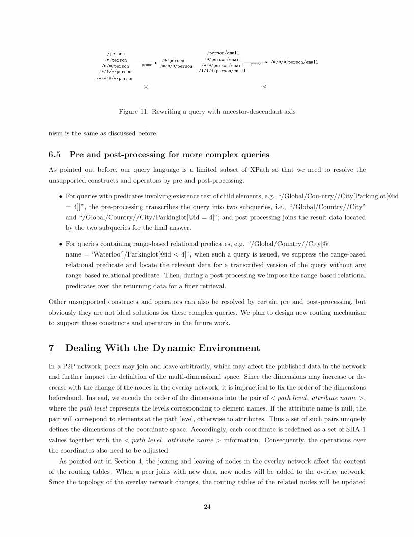
Figure 11: Rewriting a query with ancestor-descendant axis

nism is the same as discussed before.

6.5 Pre and post-processing for more complex queries

As pointed out before, our query language is a limited subset of XPath so that we need to resolve the

unsupported constructs and operators by pre and post-processing.

• For queries with predicates involving existence test of child elements, e.g. “/Global/Cou-ntry//City[Parkinglot[@id

= 4]]”, the pre-processing transcribes the query into two subqueries, i.e., “/Global/Country//City”

and “/Global/Country//City/Parkinglot[@id = 4]”; and post-processing joins the result data located

by the two subqueries for the final answer.

• For queries containing range-based relational predicates, e.g. “/Global/Country//City[@

name = ‘Waterloo’]/Parkinglot[@id < 4]”, when such a query is issued, we suppress the range-based

relational predicate and locate the relevant data for a transcribed version of the query without any

range-based relational predicate. Then, during a post-processing we impose the range-based relational

predicates over the returning data for a finer retrieval.

Other unsupported constructs and operators can also be resolved by certain pre and post-processing, but

obviously they are not ideal solutions for these complex queries. We plan to design new routing mechanism

to support these constructs and operators in the future work.

7 Dealing With the Dynamic Environment

In a P2P network, peers may join and leave arbitrarily, which may affect the published data in the network

and further impact the definition of the multi-dimensional space. Since the dimensions may increase or de-

crease with the change of the nodes in the overlay network, it is impractical to fix the order of the dimensions

beforehand. Instead, we encode the order of the dimensions into the pair of < path level, attribute name >,

where the path level represents the levels corresponding to element names. If the attribute name is null, the

pair will correspond to elements at the path level, otherwise to attributes. Thus a set of such pairs uniquely

defines the dimensions of the coordinate space. Accordingly, each coordinate is redefined as a set of SHA-1

values together with the < path level, attribute name > information. Consequently, the operations over

the coordinates also need to be adjusted.

As pointed out in Section 4, the joining and leaving of nodes in the overlay network affect the content

of the routing tables. When a peer joins with new data, new nodes will be added to the overlay network.

Since the topology of the overlay network changes, the routing tables of the related nodes will be updated

24

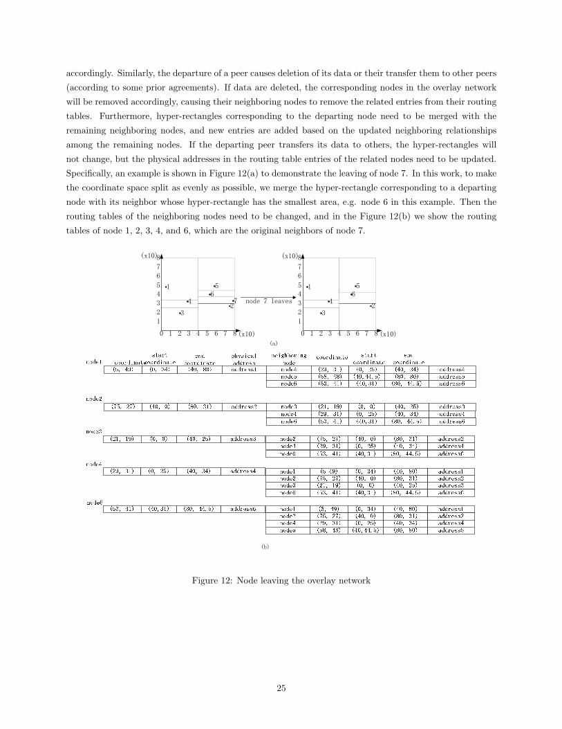
accordingly. Similarly, the departure of a peer causes deletion of its data or their transfer them to other peers

(according to some prior agreements). If data are deleted, the corresponding nodes in the overlay network

will be removed accordingly, causing their neighboring nodes to remove the related entries from their routing

tables. Furthermore, hyper-rectangles corresponding to the departing node need to be merged with the

remaining neighboring nodes, and new entries are added based on the updated neighboring relationships

among the remaining nodes. If the departing peer transfers its data to others, the hyper-rectangles will

not change, but the physical addresses in the routing table entries of the related nodes need to be updated.

Specifically, an example is shown in Figure 12(a) to demonstrate the leaving of node 7. In this work, to make

the coordinate space split as evenly as possible, we merge the hyper-rectangle corresponding to a departing

node with its neighbor whose hyper-rectangle has the smallest area, e.g. node 6 in this example. Then the

routing tables of the neighboring nodes need to be changed, and in the Figure 12(b) we show the routing

tables of node 1, 2, 3, 4, and 6, which are the original neighbors of node 7.

(a)

(b)

80 1 2 3 4 5 6 7

1

2

3

45

6

7

8

1

3

42

56

7

(x10) 80 1 2 3 4 5 6 7

1

2

3

45

6

7

8

1

3

42

56

(x10)

node 7 leaves

(x10) (x10)

Figure 12: Node leaving the overlay network

25

8 Experiments

8.1 Simulation Environment

We run tests on a physical network with Transit-Stub (TS) topology, which uses a two-level hierarchical

architecture consisting of transit domains and stub domains, where the former interconnect the latter. We

use GT-ITM [2] to generate a TS network containing 100 peers, which has one transit domain containing four

transit nodes, and eight stub domains each containing three stub nodes on average. The average inter-node

latency of the physical network is 1.0192s, which is measured by simulating TCP/IP traffic on the network

using Network Simulator-2 [5]. Network environments containing more peers are generated in a similar way.

8.2 Average hop length and routing table size for the overlay network

Although there are a number of XML query benchmarks, they do not address distributed XML query pro-

cessing. Following the parking lot example discussed earlier, we derive an XML data set from the World

Geographic Database at the University of Washington repository [7], from which we extract distinguished

paths each representing a city (e.g. shown in Figure 13). Note that the paths in the example demonstrate

some heterogeneity since different element names and attributes on defined on same path levels. We syn-

thesize parking lot id information into the paths by adding a path level with element name “Parkinglot”

and attribute name “id” at the end. Following a uniform distribution function, each city can receive up to

four parking lot ids. Altogether there are 4700 synthetic paths with parking lot id information, and some

examples are shown in Figure 14.....

/Global/Country[@name=‘Canada’]/Province[@area=‘1068582’][@name=‘Ontario’]/City[@name=‘Kitchener’]

....

/Global/Country[@name=‘China’]/Province[@name=‘Jiangsu’]/City[@population=‘2500000’][@name=‘Nanjing’]

....

/Global/Country[@name=‘United States’]/State[@name=‘New York’]/City[@name=‘Boston’]

....

Figure 13: Extracted XML paths

....

/Global/Country[@name=‘Canada’]/Province[@area=‘1068582’][@name=‘Ontario’]/City[@name=‘Kitchener’]/Parkinglot[@id=‘1’]

....

/Global/Country[@name=‘Canada’]/Province[@area=‘1068582’][@name=‘Ontario’]/City[@name=‘Kitchener’]/Parkinglot[@id=‘4’]

....

/Global/Country[@name=‘China’]/Province[@name=‘Jiangsu’]/City[@population=‘2500000’][@name=‘Nanjing’]/Parkinglot[@id=‘1’]

....

Figure 14: Parking lot data set

To demonstrate the scalability of the overlay network, we deploy the parking lot data uniformly over the

P2P network and measure the average inter-node hop length of the overlay network and the average routing

26

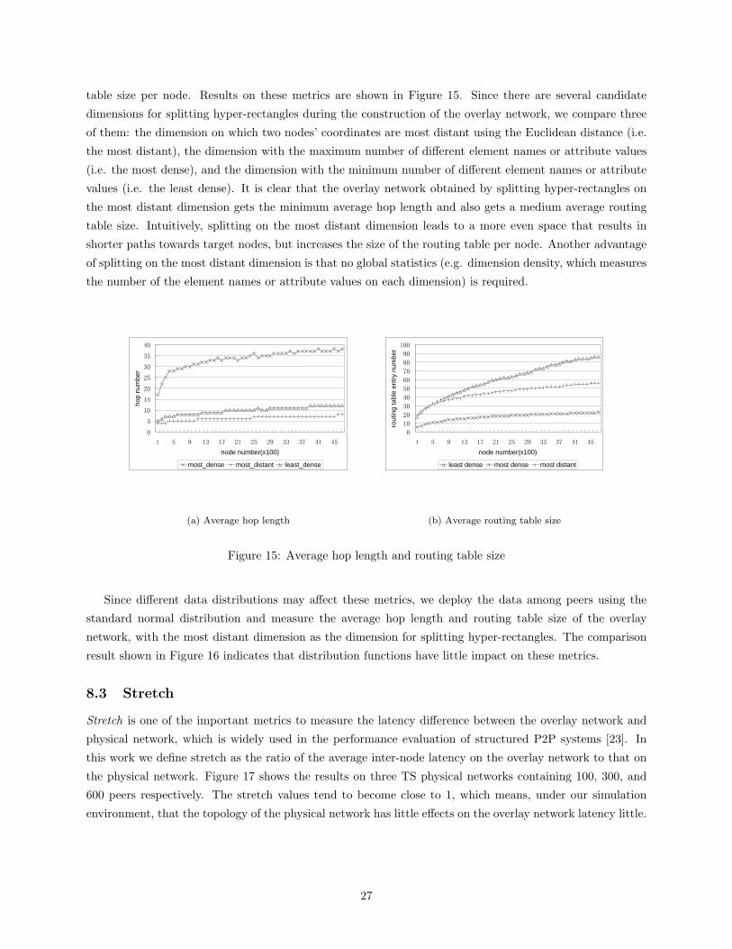
table size per node. Results on these metrics are shown in Figure 15. Since there are several candidate

dimensions for splitting hyper-rectangles during the construction of the overlay network, we compare three

of them: the dimension on which two nodes’ coordinates are most distant using the Euclidean distance (i.e.

the most distant), the dimension with the maximum number of different element names or attribute values

(i.e. the most dense), and the dimension with the minimum number of different element names or attribute

values (i.e. the least dense). It is clear that the overlay network obtained by splitting hyper-rectangles on

the most distant dimension gets the minimum average hop length and also gets a medium average routing

table size. Intuitively, splitting on the most distant dimension leads to a more even space that results in

shorter paths towards target nodes, but increases the size of the routing table per node. Another advantage

of splitting on the most distant dimension is that no global statistics (e.g. dimension density, which measures

the number of the element names or attribute values on each dimension) is required.

0

5

10

15

20

25

30

35

40

1 5 9 13 17 21 25 29 33 37 41 45

node number(x100)

hop

num

ber

most_dense most_distant least_dense

(a) Average hop length

0

10

20

30

40

50

60

70

80

90

100

1 5 9 13 17 21 25 29 33 37 41 45

node number(x100)

rout

ing

tabl

e en

try n

umbe

r

least dense most dense most distant

(b) Average routing table size

Figure 15: Average hop length and routing table size

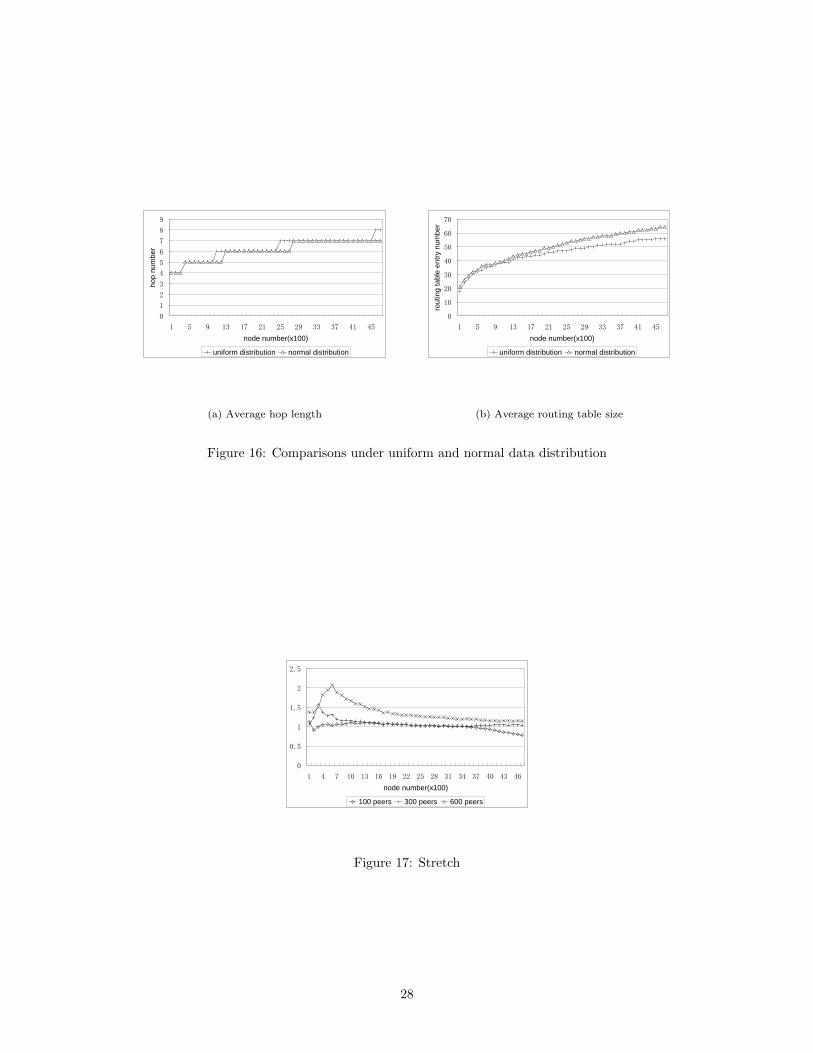
Since different data distributions may affect these metrics, we deploy the data among peers using the

standard normal distribution and measure the average hop length and routing table size of the overlay

network, with the most distant dimension as the dimension for splitting hyper-rectangles. The comparison

result shown in Figure 16 indicates that distribution functions have little impact on these metrics.

8.3 Stretch

Stretch is one of the important metrics to measure the latency difference between the overlay network and

physical network, which is widely used in the performance evaluation of structured P2P systems [23]. In

this work we define stretch as the ratio of the average inter-node latency on the overlay network to that on

the physical network. Figure 17 shows the results on three TS physical networks containing 100, 300, and

600 peers respectively. The stretch values tend to become close to 1, which means, under our simulation

environment, that the topology of the physical network has little effects on the overlay network latency little.

27

0

1

2

3

4

5

6

7

8

9

1 5 9 13 17 21 25 29 33 37 41 45

node number(x100)

hop

num

ber

uniform distribution normal distribution

(a) Average hop length

0

10

20

30

40

50

60

70

1 5 9 13 17 21 25 29 33 37 41 45

node number(x100)

rout

ing

tabl

e en

try n

umbe

r

uniform distribution normal distribution

(b) Average routing table size

Figure 16: Comparisons under uniform and normal data distribution

0

0.5

1

1.5

2

2.5

1 4 7 10 13 16 19 22 25 28 31 34 37 40 43 46

node number(x100)

100 peers 300 peers 600 peers

Figure 17: Stretch

28

8.4 Average hop length for queries

In this section we primarily test the average hop lengths for queries with wild card and ancestor-descendant

axis. We don’t consider simpler queries, e.g. queries with only parent-child axis and fully defined on all

dimensions, because the metric for these queries are reflected in the measurement of the overlay network

shown in Figure 15(a).

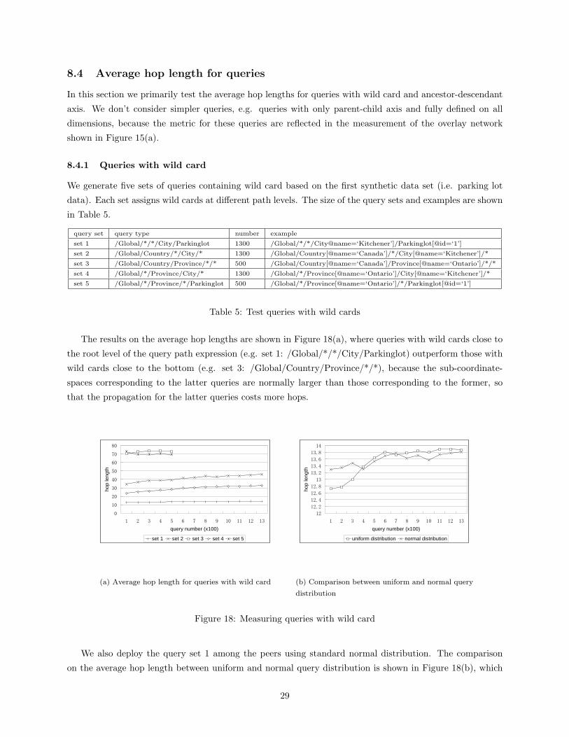
8.4.1 Queries with wild card

We generate five sets of queries containing wild card based on the first synthetic data set (i.e. parking lot

data). Each set assigns wild cards at different path levels. The size of the query sets and examples are shown

in Table 5.

query set query type number example

set 1 /Global/*/*/City/Parkinglot 1300 /Global/*/*/City@name=‘Kitchener’]/Parkinglot[@id=‘1’]

set 2 /Global/Country/*/City/* 1300 /Global/Country[@name=‘Canada’]/*/City[@name=‘Kitchener’]/*

set 3 /Global/Country/Province/*/* 500 /Global/Country[@name=‘Canada’]/Province[@name=‘Ontario’]/*/*

set 4 /Global/*/Province/City/* 1300 /Global/*/Province[@name=‘Ontario’]/City[@name=‘Kitchener’]/*

set 5 /Global/*/Province/*/Parkinglot 500 /Global/*/Province[@name=‘Ontario’]/*/Parkinglot[@id=‘1’]

Table 5: Test queries with wild cards

The results on the average hop lengths are shown in Figure 18(a), where queries with wild cards close to

the root level of the query path expression (e.g. set 1: /Global/*/*/City/Parkinglot) outperform those with

wild cards close to the bottom (e.g. set 3: /Global/Country/Province/*/*), because the sub-coordinate-

spaces corresponding to the latter queries are normally larger than those corresponding to the former, so

that the propagation for the latter queries costs more hops.

0

10

20

30

40

50

60

70

80

1 2 3 4 5 6 7 8 9 10 11 12 13

query number (x100)

hop

leng

th

set 1 set 2 set 3 set 4 set 5

(a) Average hop length for queries with wild card

12

12.2

12.4

12.6

12.8

13

13.2

13.4

13.6

13.8

14

1 2 3 4 5 6 7 8 9 10 11 12 13

query number (x100)

hop

leng

th

uniform distribution normal distribution

(b) Comparison between uniform and normal query

distribution

Figure 18: Measuring queries with wild card

We also deploy the query set 1 among the peers using standard normal distribution. The comparison

on the average hop length between uniform and normal query distribution is shown in Figure 18(b), which

29

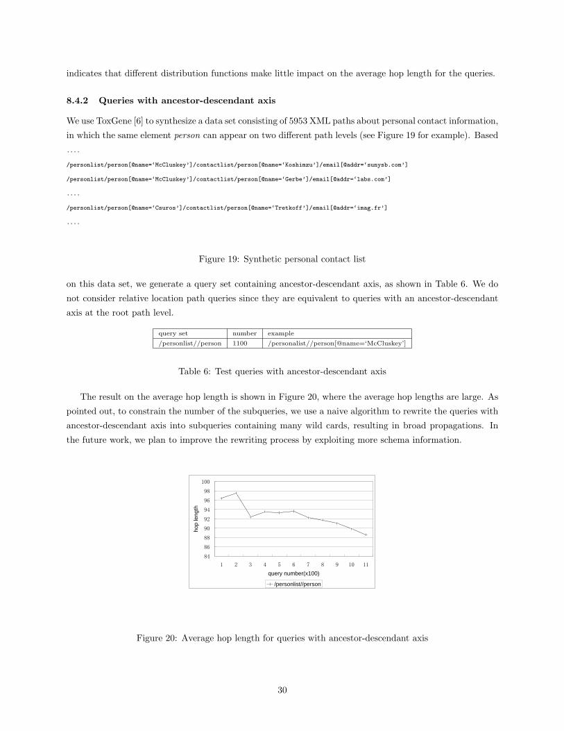
indicates that different distribution functions make little impact on the average hop length for the queries.

8.4.2 Queries with ancestor-descendant axis

We use ToxGene [6] to synthesize a data set consisting of 5953 XML paths about personal contact information,

in which the same element person can appear on two different path levels (see Figure 19 for example). Based

....

/personlist/person[@name=‘McCluskey’]/contactlist/person[@name=‘Koshimzu’]/email[@addr=‘sunysb.com’]

/personlist/person[@name=‘McCluskey’]/contactlist/person[@name=‘Gerbe’]/email[@addr=‘labs.com’]

....

/personlist/person[@name=‘Csuros’]/contactlist/person[@name=‘Tretkoff’]/email[@addr=‘imag.fr’]

....

Figure 19: Synthetic personal contact list

on this data set, we generate a query set containing ancestor-descendant axis, as shown in Table 6. We do

not consider relative location path queries since they are equivalent to queries with an ancestor-descendant

axis at the root path level.

query set number example

/personlist//person 1100 /personalist//person[@name=‘McCluskey’]

Table 6: Test queries with ancestor-descendant axis

The result on the average hop length is shown in Figure 20, where the average hop lengths are large. As

pointed out, to constrain the number of the subqueries, we use a naive algorithm to rewrite the queries with

ancestor-descendant axis into subqueries containing many wild cards, resulting in broad propagations. In

the future work, we plan to improve the rewriting process by exploiting more schema information.

84

86

88

90

92

94

96

98

100

1 2 3 4 5 6 7 8 9 10 11

query number(x100)

hop

leng

th

/personlist//person

Figure 20: Average hop length for queries with ancestor-descendant axis

30

9 Conclusion

We discussed the design of a novel data locating mechanism for distributed XML query processing over P2P

network. The primary problem we address is how to locate distributed XML data relevant to XML queries

without any centralized mechanism or flooding the network. To deal with these problems, we follow the

multi-hop style of the structured P2P file sharing systems, but is different in that we encode the hierarchical

information of the XML data into the overlay network, so that hierarchical routing keys (i.e. XML path

expressions) are supported. Furthermore, our data locating mechanism does not employ any centralized

catalogs. To avoid flooding the network with XML queries, we use a technique that propagates queries

within a limited sub-network to improve the performance.

Certain limitations exist in the current design. Since we use SHA-1 to map element names and attribute

values into the coordinate space, the data locating mechanism can not deal with range queries. Moreover,

order sensitive constructs in the XPath language are not defined in either distributed XML data definition

language or query definition language, so they are not supported in this work. These will be addressed in

follow-up work.

Furthermore, in this work we constrain each path for the published distributed XML data to only contain

parent-child axis. To support data with more heterogeneity (e.g. twig patterns [12]), a more complicated

distributed XML data definition language is needed. If we avoid a naive approach to decompose twig patterns

into parent-child and ancestor-descendant axes, the overlay network needs to be redesigned to encode more

complicated hierarchical structure information.

Finally, the experiments conducted in the simulated network environment show the effectiveness of our

approach. However, we plan to do more performance evaluation on real network environment (e.g. Planetlab

testbed [4]).

References

[1] Active XML. http://www-rocq.inria.fr/gemo/Gemo/ Projects/axml/.

[2] Georgia Tech Internetwork Topology Models. http://www.cc.gatech.edu/fac/Ellen.Zegura/graphs.html.

[3] Internet-scale Resource-Intensive Sensor Network Service. http://www.intel-iris.net/.

[4] Planetlab. http://www.planet-lab.org.

[5] The Network Simulator 2. http://www.isi.edu/nsnam/ns/ns-topogen.html.

[6] Toxgene-the TOX XML Data Generator. http://www.cs.toronto.edu/tox/toxgene/.

[7] XML data repository. http://www.cs.washington.edu/research/xmldatasets/.

[8] Web Services Description Language (WSDL). http://www.w3.org/TR/wsdl, March 2001.

[9] Simple Object Access Protocol (SOAP). http://www.w3.org/TR/soap, June 2003.

[10] Scott Boag, Don Chamberlin, Mary F. Fernandez, Daniela Florescu, Jonathan Robie, and Jerome

Simeon. Xquery 1.0 : An xml query language, w3c working draft. http://www.w3.org/TR/xquery,

August 2002.

31

[11] J-M. Bremer and M. Gertz. On distributing XML repositories. In Proc. 6th Int. Workshop on the World

Wide Web and Databases (WebDB), pages 73–78, 2003.

[12] N. Bruno, N. Koudas, and D. Srivastava. Holistic twig joins: optimal XML pattern matching. In Proc.

ACM SIGMOD Int. Conf. on Management of Data, pages 310–321, 2002.

[13] J. Clark and S. DeRose. XML Path Language (XPath) Version 1.0 W3C Recommendation.

http://www.w3.org/TR/xpath, November 1999.

[14] A. Deshpande, S. K. Nath, P. B. Gibbons, and S. Seshan. Cache-and-query for wide area sensor

databases. In Proc. ACM SIGMOD Int. Conf. on Management of Data, pages 503–514, 2003.

[15] Y. Diao, S. Rizvi, and M. J. Franklin. Towards an Internet-Scale XML Dissemination Service. In Proc.

30th Int. Conf. on Very Large Data Bases, pages 612–623, 2004.

[16] L. Fegaras, D. Levine, S. Bose, and V. Chaluvadi. Query processing of streamed XML data. In Proc.

11th Int. Conf. on Information and Knowledge Management, pages 126–133, 2002.

[17] L. Galanis, Y. Wang, S. R. Jeffery, and D. J. DeWitt. Locating data sources in large distributed systems.

In Proc. 29th Int. Conf. on Very Large Data Bases, pages 874–885, 2003.

[18] P. Grosso and D. Veillard. XML Fragment Interchange W3C Working Draft.

http://www.w3.org/TR/xml-fragment.html, February 2001.

[19] G. Koloniari and E. Pitoura. Content-based routing of path queries in peer-to-peer systems. In Advances

in Database Technology — EDBT’04, pages 29–47, 2004.

[20] M. Kratky, J. Pokorny, and V. Snasel. Indexing XML Data with UB-trees. In In Proceedings of 6th

East-European Conference on Advances in Databases and Information Systems, 2002.

[21] D. L. Lee, Y. M. Kim, and G. Patel. Efficient signature file methods for text retrieval. In IEEE Trans.

Knowledge and Data Eng., pages 423–435, 1995.

[22] S. Ratnasamy, P. Francis, M. Handley, R. Karp, and S. Shenker. A scalable content-addressable network.

In Proc. of the ACM SIGCOMM 2001 Conference on Applications, Technologies, Architectures, and

Protocols for Computer Communication, pages 161–172, 2001.

[23] S. Ratnasamy, M. Handley, R. Karp, and S. Shenker. Topologically-aware overlay construction and

server selection. In The 21st Annual Joint Conference of the IEEE Computer and Communications

Societies, 2002.

[24] A. Rowstron and P. Druschel. Pastry: Scalable, decentralized object location, and routing for large-scale

peer-to-peer systems. In Proc. Middleware 2001, IFIP/ACM International Conference on Distributed

Systems Platforms, pages 329–350, 2001.

[25] O. D. Sahin, A. Gupta, D. Agrawal, and A. Abbadi. Query processing over peer to peer data sharing

systems. Technical Report UCSB/CSD-2002-28, University of California at Santa Barbara, 2002.

32

[26] I. Stoica, R. Morris, D. Liben-Nowell, D. R. Karger, M. F. Kaashoek, F. Dabek, and H. Balakrish-

nan. Chord: a scalable peer-to-peer lookup protocol for internet applications. In Proc. of the ACM

SIGCOMM 2001 Conference on Applications, Technologies, Architectures, and Protocols for Computer

Communication, pages 149–160, 2001.

[27] D. Suciu. Distributed query evaluation on semistructured data. ACM Trans. Database Sys., pages 1–62,

2002.

[28] the National Institute of Standards and Technology (NIST). Secure hash standard.

http://www.itl.nist.gov/fipspubs/fip180-1.htm, August 2002.

[29] B. Y. Zhao, J. Kubiatowicz, and A. D. Joseph. Tapestry: An infrastructure for faulttolerant wide-area

location and routing. Technical Report UCB/CSD-01-1141, University of California, Berkeley, 2001.

33