A Critique of Partial Least Squares, and a Preliminary Assessement of an Alternative Estimation Method

�������������� �����������������������������

���������������������������������������������������������������������� ��!�����"���#�����$�

����

����

����

����

����

����

����

����

�� ��

Sprott Letters Working Papers � Occasional Reports � Article Reprints �

Frontiers in Business Research and Practice �

A Critique of Partial Least Squares, and a Preliminary Assessement

of an Alternative Estimation Method��������

����

D. Roland Thomas, Irene R.R. Lu, and Marzena Cedzynski����

February 2007 SL 2007-002

About the authors Irene R. R. Lu is Assistant Professor at the School of Administrative Studies, York University, and a graduate of the Ph.D. in Management program of the Sprott School of Business. D. Roland Thomas is Professor of Quantitative Methods, and Marzena Cedzynski a doctoral candidate, in the Sprott School of Business.

The research of the first author was supported by grants from the Natural Sciences and Engineering Research Council of Canada and from the National Program on Complex Data Structures.

Abstract Partial least squares (PLS) is sometimes used as an alternative to covariance-based structural equation modeling (SEM). This paper briefly reviews currently available SEM techniques, and provides a critique of the perceived advantages of PLS over covariance-based SEM as commonly cited by PLS users. Specific attention is drawn to the primary disadvantage of PLS, namely the lack of consistency of its parameter estimates. The instrumental variables (IV) / two stage least squares (2SLS) method of estimation is then described and presented as a potential alternative to PLS that might yield its perceived advantages without succumbing to its primary disadvantage. Preliminary simulation results show that: PLS parameter estimates exhibit substantial bias when the number of items is moderate; SEM-based methods yield lower bias; and IV/2SLS estimates may indeed provide a viable ordinary least squares (OLS)-based alternative to PLS.

Sprott Letters Working Papers

A Critique of Partial Least Squares, and a Preliminary Assessement

of an Alternative Estimation Method

D. Roland Thomas, Sprott School of Business Irene R.R. Lu, York University

Marzena Cedzynski, Sprott School of Business

SL 2007-002 Ottawa, Canada � February 2007

Corresponding author: Dr. Irene R.R. Lu, School of Administrative Studies, Atkinson Building, York University, 4700 Keele Street, Toronto, Canada M3J 1P3. (Phone: 416-736-2100 ext. 22414, E-mail: [email protected]). © By the authors. Please do not quote or reproduce without permission.

Sprott Letters (Print) ISSN 1912-6026 Sprott Letters (Online) ISSN 1912-6034

Sprott Letters includes four series: Working Papers, Occasional Reports, Article Reprints, and Frontiers in Business Research and Practice.

For more information please visit “Faculty & Research” at http://sprott.carleton.ca/.

1

A Critique of Partial Least Squares,

and a Preliminary Assessement of an Alternative Estimation Method

Introduction

Structural equation modelling (SEM) is now a popular technique in the social,

behavioural and business sciences for exploring and assessing complex linear relationships

among many variables, in particular between endogenous and exogenous latent variables that

cannot be directly observed but that must be inferred by means of manifest indicator variables,

i.e., variables measured without error. The main category of SEM techniques, which is based on

fitting the model-implied covariance matrix of the manifest variables (or items) to the empirically

determined covariance matrix, is implemented in a number of software package including Mplus

(Muthén & Muthén, 2001) and LISREL (Jöreskog & Sörbom, 1996). The covariance-based

approach to SEM is of particular interest because it explicitly models the measurement error

associated with each latent variable and therefore ensures that estimates of the SEM parameters

are consistent. Consistency of estimation is an important (some would say essential) statistical

property which states that with high probability, an estimate will become closer and closer to its

true value for increasingly large sample sizes. An alternative approach to SEM modeling called

partial least squares (PLS) was developed by Wold (1982, 1985), based on earlier work of his

dating from the mid-1960’s (for references see Tenenhaus, Vinzi, Chatelin, and Lauro, 2005).

PLS uses an iterative application of ordinary least squares (OLS) to first estimate values of the

latent variables for each individual, followed by OLS estimation of model parameters based on

the latent variable values, or scores. Jöreskog and Wold (1982) and Wold (1982, 1985) referred

to the PLS technique as “soft modelling”, because it did not require the “hard “ distributional

assumptions of maximum likelihood (ML)-SEM, and because it used a sub-optimal estimation

technique that is faster to run than ML-SEM and which therefore allowed for more user

interaction. They claimed that PLS and ML-SEM provided similar results, i.e., estimates for

which numerical differences “cannot or should not be substantial” (Jöreskog & Wold, 1982,

p.266), a claim is difficult to justify for reasons that will be discussed.

2

Other differences between PLS and covariance-based SEM have been identified by

Jöreskog and Wold (1982) and numerous other authors, and a brief summary of this literature

will be provided later in the paper. One particular difference mentioned by Jöreskog and Wold

(1982) and Wold (1982, 1985) is that PLS parameter estimates are not consistent in the usual

large sample sense. They state that PLS estimates will only converge to their true values for large

samples if the number of items associated with each latent variable is also large, an additional

requirement that they refer to as “consistency at large”. Lu (2004) and Lu, Thomas, and Zumbo

(2005) referred to the bias arising from a failure of “consistency at large” as “finite item bias”.

This lack of consistency is well known from the study of the errors arising in regression analysis

when measurement error in predictor variables is ignored, as discussed in detail by Fuller (1987),

for example. This issue has been raised in the technical literature pertaining to PLS (see, for

example, Dikstra, 1983; Schneeweiss, 1993) as well as in the expository literature on PLS (see

Barclay, Higgins, and Thompson, 1995; Chin, 1998). But apart from some cautions by Chin

(1995, 1998), the anecdotal and literary evidence is that the users and proponents of PLS believe

that it offers a number of practical advantages over covariance-based SEM methods, and that they

are unaware of the problem of finite item bias that arises from a violation of consistency at large.

Recent evidence of the low visibility of this issue is provided by the detailed review of PLS by

Tenenhaus et al., (2005) which makes no mention of consistency at large or related issues.

The focus of this paper is three-fold. First, after reviewing the competing SEM techniques

and providing some technical details relating to consistency at large, the paper provides a critique

of the perceived advantages of PLS over covariance-based SEM as commonly cited by PLS

users. The list of the perceived advantages is based on a small survey of the applied literature.

Second, the instrumental variables (IV) / two stage least squares (2SLS) method of estimation

will be described and presented as a potential alternative to PLS that might yield some of its

perceived advantages without succumbing to its primary disadvantage. Finally, some simulation

results will be presented that demonstrate: (i) that PLS parameter estimates exhibit substantial

bias when the number of items is moderate, (ii) that SEM-based methods yield lower bias, and

(iii) that IV estimates may provide a viable, ordinary least squares (OLS)-based alternative to

PLS. The paper is intended as a preliminary report on the authors’ investigation of PLS

3

modeling, and it is hoped that it will stimulate constructive discussion of the issues and spur

further research on what are important practical issues.

A Latent Regression Model and the Primary SEM Analysis Strategies

Multiple Latent Regression

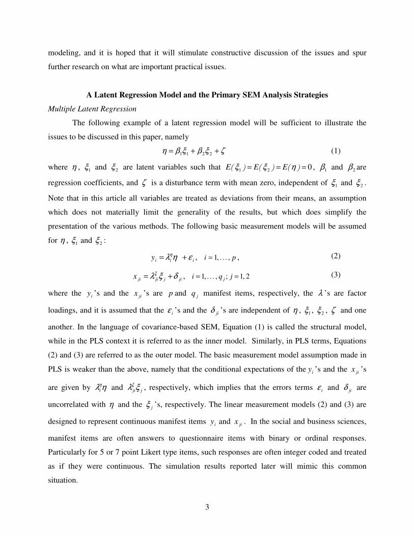
The following example of a latent regression model will be sufficient to illustrate the

issues to be discussed in this paper, namely

ζξβξβη ++= 2211 (1)

where η , 1ξ and 2ξ are latent variables such that 021 === ������ ηξξ EEE , 1β and 2β are

regression coefficients, and ζ is a disturbance term with mean zero, independent of 1ξ and 2ξ .

Note that in this article all variables are treated as deviations from their means, an assumption

which does not materially limit the generality of the results, but which does simplify the

presentation of the various methods. The following basic measurement models will be assumed

for η , 1ξ and 2ξ :

iiiy εηλη += , pi , . . . ,1 = , (2)

jijjijix δξλξ += , 2 ,1 ; , . . . ,1 == jqi j (3)

where the iy ’s and the jix ’s are p and jq manifest items, respectively, the λ ’s are factor

loadings, and it is assumed that the iε ’s and the jiδ ’s are independent of η , 1ξ , 2ξ , ζ and one

another. In the language of covariance-based SEM, Equation (1) is called the structural model,

while in the PLS context it is referred to as the inner model. Similarly, in PLS terms, Equations

(2) and (3) are referred to as the outer model. The basic measurement model assumption made in

PLS is weaker than the above, namely that the conditional expectations of the iy ’s and the jix ’s

are given by ηληi and jjiξλξ , respectively, which implies that the errors terms iε and jiδ are

uncorrelated with η and the jξ ’s, respectively. The linear measurement models (2) and (3) are

designed to represent continuous manifest items iy and jix . In the social and business sciences,

manifest items are often answers to questionnaire items with binary or ordinal responses.

Particularly for 5 or 7 point Likert type items, such responses are often integer coded and treated

as if they were continuous. The simulation results reported later will mimic this common

situation.

4

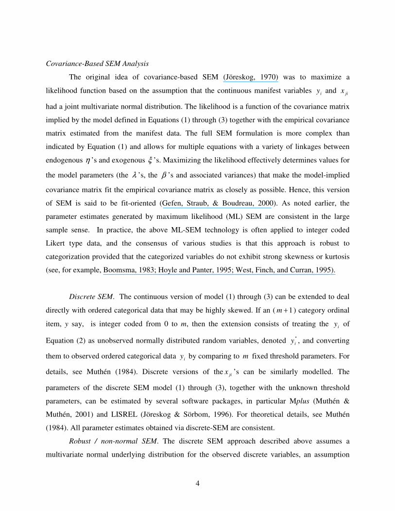
Covariance-Based SEM Analysis

The original idea of covariance-based SEM (Jöreskog, 1970) was to maximize a

likelihood function based on the assumption that the continuous manifest variables iy and jix

had a joint multivariate normal distribution. The likelihood is a function of the covariance matrix

implied by the model defined in Equations (1) through (3) together with the empirical covariance

matrix estimated from the manifest data. The full SEM formulation is more complex than

indicated by Equation (1) and allows for multiple equations with a variety of linkages between

endogenous η ’s and exogenous ξ ’s. Maximizing the likelihood effectively determines values for

the model parameters (the λ ’s, the β ’s and associated variances) that make the model-implied

covariance matrix fit the empirical covariance matrix as closely as possible. Hence, this version

of SEM is said to be fit-oriented (Gefen, Straub, & Boudreau, 2000). As noted earlier, the

parameter estimates generated by maximum likelihood (ML) SEM are consistent in the large

sample sense. In practice, the above ML-SEM technology is often applied to integer coded

Likert type data, and the consensus of various studies is that this approach is robust to

categorization provided that the categorized variables do not exhibit strong skewness or kurtosis

(see, for example, Boomsma, 1983; Hoyle and Panter, 1995; West, Finch, and Curran, 1995).

Discrete SEM. The continuous version of model (1) through (3) can be extended to deal

directly with ordered categorical data that may be highly skewed. If an ( 1+m ) category ordinal

item, y say, is integer coded from 0 to m, then the extension consists of treating the iy of

Equation (2) as unobserved normally distributed random variables, denoted �

iy , and converting

them to observed ordered categorical data iy by comparing to m fixed threshold parameters. For

details, see Muthén (1984). Discrete versions of the jix ’s can be similarly modelled. The

parameters of the discrete SEM model (1) through (3), together with the unknown threshold

parameters, can be estimated by several software packages, in particular Mplus (Muthén &

Muthén, 2001) and LISREL (Jöreskog & Sörbom, 1996). For theoretical details, see Muthén

(1984). All parameter estimates obtained via discrete-SEM are consistent.

Robust / non-normal SEM. The discrete SEM approach described above assumes a

multivariate normal underlying distribution for the observed discrete variables, an assumption

5

that is difficult to verify. Other approaches to non-normal observed items have been developed

that avoid this assumption. An early attempt by Browne (1984) featured an asymptotically

efficient and distribution free (ADF) approach based on weighted least squares (WLS), but more

recent work (Muthén & Kaplan, 1992) has shown that the ADF method requires prohibitively

large sample sizes. Variants of the ADF method have been developed that do not require such

large samples. Browne (1984) also proved that ML-SEM methods yield consistent parameter

estimates under non-normality, but that their standard error estimates are not consistent. Attention

has therefore been focussed on deriving corrected standard errors for ML estimates under non-

normality. For details on these so-called pseudo ML (or PML) methods, see Arminger and

Schoenberg (1989). Related “minimum-distance” (MD) methods based on weighted least

squares have also been developed that yield consistent parameter and standard error estimates and

require significantly smaller sample sizes than ADF. For PML and MD methods, Satorra and

Bentler (1994) have developed corrections that can be applied to the goodness of fit statistic that

recover its approximate chi-squared distribution for non-normal manifest items.

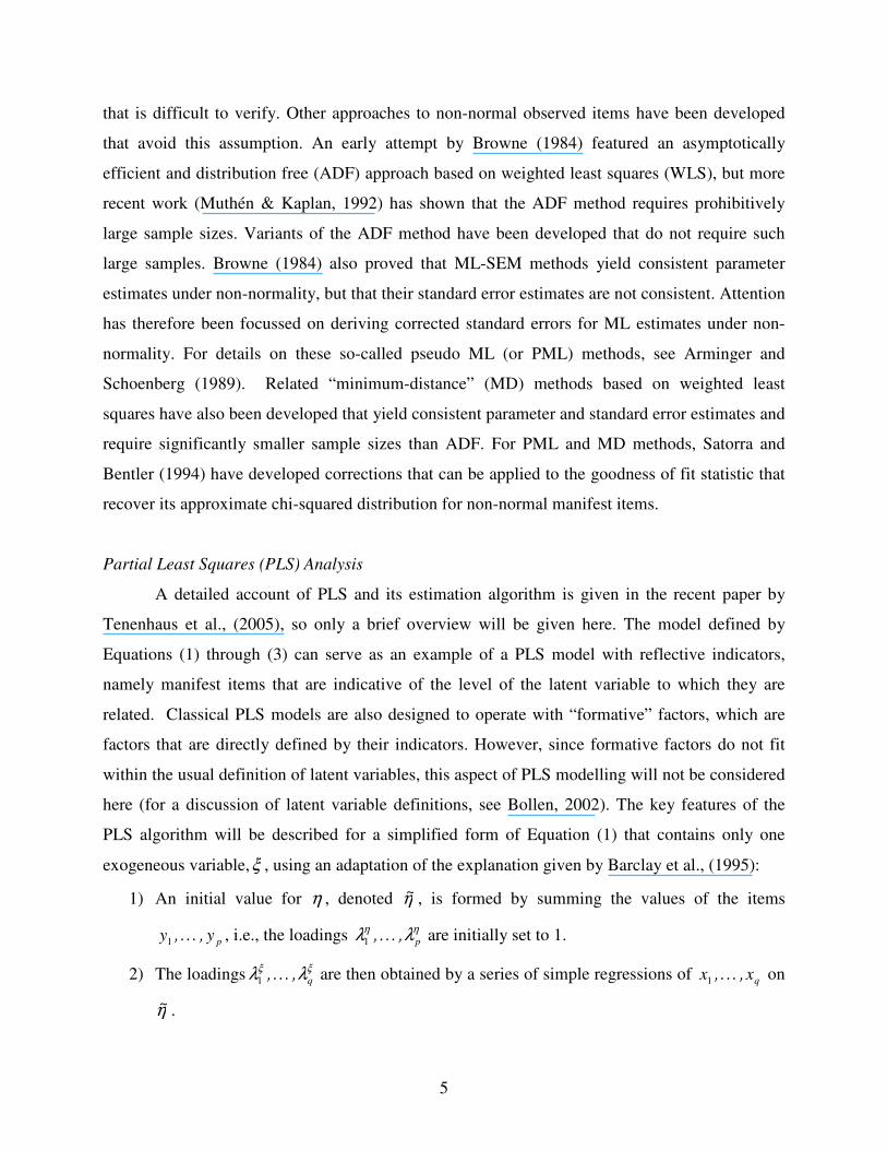
Partial Least Squares (PLS) Analysis

A detailed account of PLS and its estimation algorithm is given in the recent paper by

Tenenhaus et al., (2005), so only a brief overview will be given here. The model defined by

Equations (1) through (3) can serve as an example of a PLS model with reflective indicators,

namely manifest items that are indicative of the level of the latent variable to which they are

related. Classical PLS models are also designed to operate with “formative” factors, which are

factors that are directly defined by their indicators. However, since formative factors do not fit

within the usual definition of latent variables, this aspect of PLS modelling will not be considered

here (for a discussion of latent variable definitions, see Bollen, 2002). The key features of the

PLS algorithm will be described for a simplified form of Equation (1) that contains only one

exogeneous variable,ξ , using an adaptation of the explanation given by Barclay et al., (1995):

1) An initial value for η , denoted η� , is formed by summing the values of the items

pyy ����� 1 , i.e., the loadings ηη λλ p����� 1 are initially set to 1.

2) The loadings ξξ λλ q����� 1 are then obtained by a series of simple regressions of qxx ����� 1 on

η� .

6

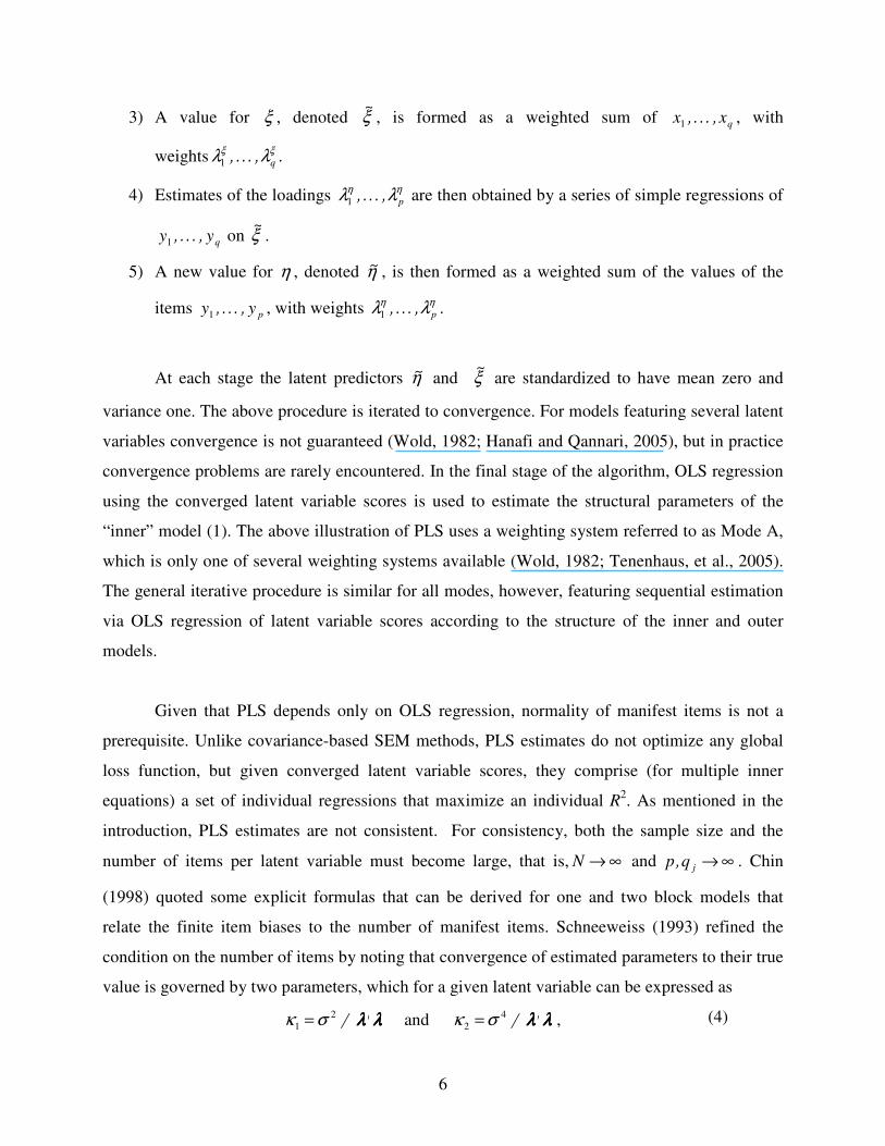
3) A value for ξ , denoted ξ� , is formed as a weighted sum of qxx ����� 1 , with

weights ξξ λλ q����� 1 .

4) Estimates of the loadings ηη λλ p����� 1 are then obtained by a series of simple regressions of

qyy ����� 1 on ξ� .

5) A new value for η , denoted η� , is then formed as a weighted sum of the values of the

items pyy ����� 1 , with weights ηη λλ p����� 1 .

At each stage the latent predictors η� and ξ� are standardized to have mean zero and

variance one. The above procedure is iterated to convergence. For models featuring several latent

variables convergence is not guaranteed (Wold, 1982; Hanafi and Qannari, 2005), but in practice

convergence problems are rarely encountered. In the final stage of the algorithm, OLS regression

using the converged latent variable scores is used to estimate the structural parameters of the

“inner” model (1). The above illustration of PLS uses a weighting system referred to as Mode A,

which is only one of several weighting systems available (Wold, 1982; Tenenhaus, et al., 2005).

The general iterative procedure is similar for all modes, however, featuring sequential estimation

via OLS regression of latent variable scores according to the structure of the inner and outer

models.

Given that PLS depends only on OLS regression, normality of manifest items is not a

prerequisite. Unlike covariance-based SEM methods, PLS estimates do not optimize any global

loss function, but given converged latent variable scores, they comprise (for multiple inner

equations) a set of individual regressions that maximize an individual R2. As mentioned in the

introduction, PLS estimates are not consistent. For consistency, both the sample size and the

number of items per latent variable must become large, that is, ∞→N and ∞→jqp� . Chin

(1998) quoted some explicit formulas that can be derived for one and two block models that

relate the finite item biases to the number of manifest items. Schneeweiss (1993) refined the

condition on the number of items by noting that convergence of estimated parameters to their true

value is governed by two parameters, which for a given latent variable can be expressed as

�21 σκ = λλλλλλλλ� and �4

2 σκ = λλλλλλλλ� , (4)

7

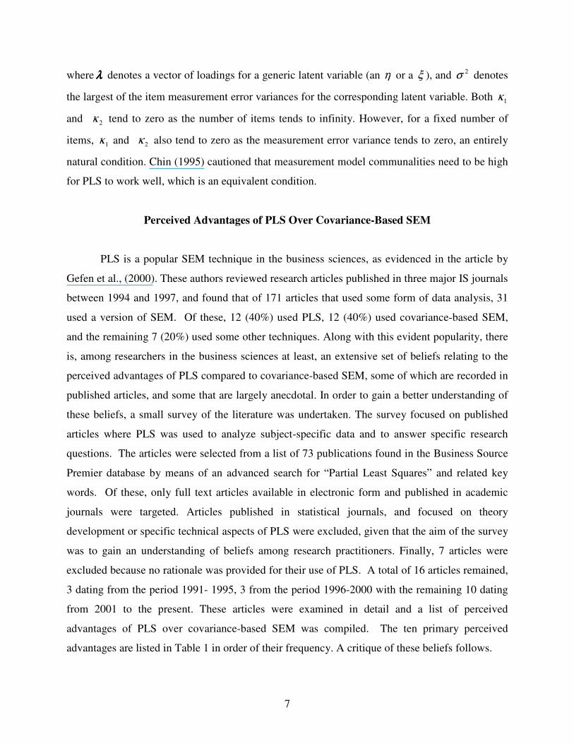
where λλλλ denotes a vector of loadings for a generic latent variable (an η or a ξ ), and 2σ denotes

the largest of the item measurement error variances for the corresponding latent variable. Both 1κ

and 2κ tend to zero as the number of items tends to infinity. However, for a fixed number of

items, 1κ and 2κ also tend to zero as the measurement error variance tends to zero, an entirely

natural condition. Chin (1995) cautioned that measurement model communalities need to be high

for PLS to work well, which is an equivalent condition.

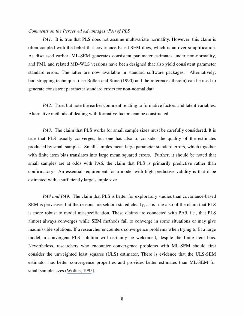
Perceived Advantages of PLS Over Covariance-Based SEM

PLS is a popular SEM technique in the business sciences, as evidenced in the article by

Gefen et al., (2000). These authors reviewed research articles published in three major IS journals

between 1994 and 1997, and found that of 171 articles that used some form of data analysis, 31

used a version of SEM. Of these, 12 (40%) used PLS, 12 (40%) used covariance-based SEM,

and the remaining 7 (20%) used some other techniques. Along with this evident popularity, there

is, among researchers in the business sciences at least, an extensive set of beliefs relating to the

perceived advantages of PLS compared to covariance-based SEM, some of which are recorded in

published articles, and some that are largely anecdotal. In order to gain a better understanding of

these beliefs, a small survey of the literature was undertaken. The survey focused on published

articles where PLS was used to analyze subject-specific data and to answer specific research

questions. The articles were selected from a list of 73 publications found in the Business Source

Premier database by means of an advanced search for “Partial Least Squares” and related key

words. Of these, only full text articles available in electronic form and published in academic

journals were targeted. Articles published in statistical journals, and focused on theory

development or specific technical aspects of PLS were excluded, given that the aim of the survey

was to gain an understanding of beliefs among research practitioners. Finally, 7 articles were

excluded because no rationale was provided for their use of PLS. A total of 16 articles remained,

3 dating from the period 1991- 1995, 3 from the period 1996-2000 with the remaining 10 dating

from 2001 to the present. These articles were examined in detail and a list of perceived

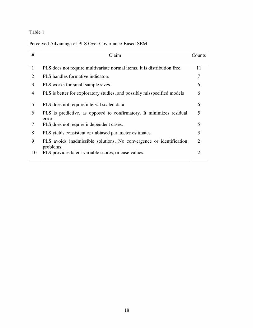
advantages of PLS over covariance-based SEM was compiled. The ten primary perceived

advantages are listed in Table 1 in order of their frequency. A critique of these beliefs follows.

8

Comments on the Perceived Advantages (PA) of PLS

PA1. It is true that PLS does not assume multivariate normality. However, this claim is

often coupled with the belief that covariance-based SEM does, which is an over-simplification.

As discussed earlier, ML-SEM generates consistent parameter estimates under non-normality,

and PML and related MD-WLS versions have been designed that also yield consistent parameter

standard errors. The latter are now available in standard software packages. Alternatively,

bootstrapping techniques (see Bollen and Stine (1990) and the references therein) can be used to

generate consistent parameter standard errors for non-normal data.

PA2. True, but note the earlier comment relating to formative factors and latent variables.

Alternative methods of dealing with formative factors can be constructed.

PA3. The claim that PLS works for small sample sizes must be carefully considered. It is

true that PLS usually converges, but one has also to consider the quality of the estimates

produced by small samples. Small samples mean large parameter standard errors, which together

with finite item bias translates into large mean squared errors. Further, it should be noted that

small samples are at odds with PA6, the claim that PLS is primarily predictive rather than

confirmatory. An essential requirement for a model with high predictive validity is that it be

estimated with a sufficiently large sample size.

PA4 and PA9. The claim that PLS is better for exploratory studies than covariance-based

SEM is pervasive, but the reasons are seldom stated clearly, as is true also of the claim that PLS

is more robust to model misspecification. These claims are connected with PA9, i.e., that PLS

almost always converges while SEM methods fail to converge in some situations or may give

inadmissible solutions. If a researcher encounters convergence problems when trying to fit a large

model, a convergent PLS solution will certainly be welcomed, despite the finite item bias.

Nevertheless, researchers who encounter convergence problems with ML-SEM should first

consider the unweighted least squares (ULS) estimator. There is evidence that the ULS-SEM

estimator has better convergence properties and provides better estimates than ML-SEM for

small sample sizes (Wolins, 1995).

9

PA5. The apparently common belief that PLS does not require interval scaled data is

bizarre, and totally incorrect. Nothing in the theory of OLS regression justifies such a claim.

PA6 and PA10. The claim that PLS is predictive as opposed to confirmatory derives from

the use of OLS regression which minimizes 2R for each estimated equation in the system.

However, the principle of least squares is also fundamental to confirmatory techniques such as

analysis of variance (ANOVA), so that the predictive claim should be treated cautiously. Many

studies based on PLS discuss their results entirely in confirmatory terms (see, for example,

Barclay et al., 1995) and do not use predictive measures, e.g., cross-validation. Also, contrary to

the implication of PA10 that only PLS generates latent variable scores, scores can be predicted

once the parameters of the measurement models (2) and (3) have been estimated by covariance-

based SEM techniques. The “regression” method for generating factor scores yields individual

predictions (scores) that minimize the mean-squared error of prediction, i.e., they minimize 2�� ηηηηηηηη −E . Thus covariance-based SEM can also be said to be prediction oriented. The package

Mplus offers a wide range of scoring methods, for both continuous and discrete SEM methods.

PA7. OLS methods applied to variables that are free of measurement error do yield

consistent parameter estimates even when observations are correlated. However, corresponding

parameter standard errors will be biased. PLS uses resampling methods to estimate these standard

errors, and standard resampling methods require independent, identically distributed

observations. Thus, if finite item bias is small enough to be ignored, the claim will be correct if

applied to point estimates, but false whenever inferential techniques are applied.

PA8. This belief is false, as described in the earlier description of PLS, unless the number

of items is very large and / or unless the measurement error is negligible.

Instrumental Variables (IV) / Two Stage Least Squares (2SLS)

Though popular in econometrics, the IV/2SLS approach to estimation has seen relatively

limited use in the fields of factor analysis and structural equation modeling. The IV/2SLS

approach to estimation in fact refers to a family of related techniques, among which several

10

variants have been proposed for latent variable models, for example those of Bentler (1982),

Lance, Cornwell, and Mulaik (1988), and Jöreskog and Sörbom (1996), the latter being

implemented in the LISREL program. More recently, Bollen (1996) proposed a flexible

IV/2SLS technique that differs from these earlier versions and that can easily be applied to

estimate the parameters of a single structural equation or of a system of such equations. In this

paper, the acronym IV/2SLS will refer to Bollen’s (1996) technique, unless otherwise noted.

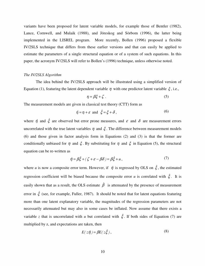
The IV/2SLS Algorithm

The idea behind the IV/2SLS approach will be illustrated using a simplified version of

Equation (1), featuring the latent dependent variable η with one predictor latent variable ξ , i.e.,

ζβξη += . (5)

The measurement models are given in classical test theory (CTT) form as

εηη += and δξξ += , (6)

where η and ξ are observed but error prone measures, and ε and δ are measurement errors

uncorrelated with the true latent variables η and ξ . The difference between measurement models

(6) and those given in factor analysis form in Equations (2) and (3) is that the former are

conditionally unbiased for η and ξ . By substituting for η and ξ in Equation (5), the structural

equation can be re-written as

u+=−++= ξββδεζξβη �� , (7)

where u is now a composite error term. However, if η is regressed by OLS on ξ , the estimated

regression coefficient will be biased because the composite error u is correlated with ξ . It is

easily shown that as a result, the OLS estimate β is attenuated by the presence of measurement

error in ξ (see, for example, Fuller, 1987). It should be noted that for latent equations featuring

more than one latent explanatory variable, the magnitudes of the regression parameters are not

necessarily attenuated but may also in some cases be inflated. Now assume that there exists a

variable z that is uncorrelated with u but correlated with ξ . If both sides of Equation (7) are

multiplied by z, and expectations are taken, then

���� ξβη zEzE = , (8)

11

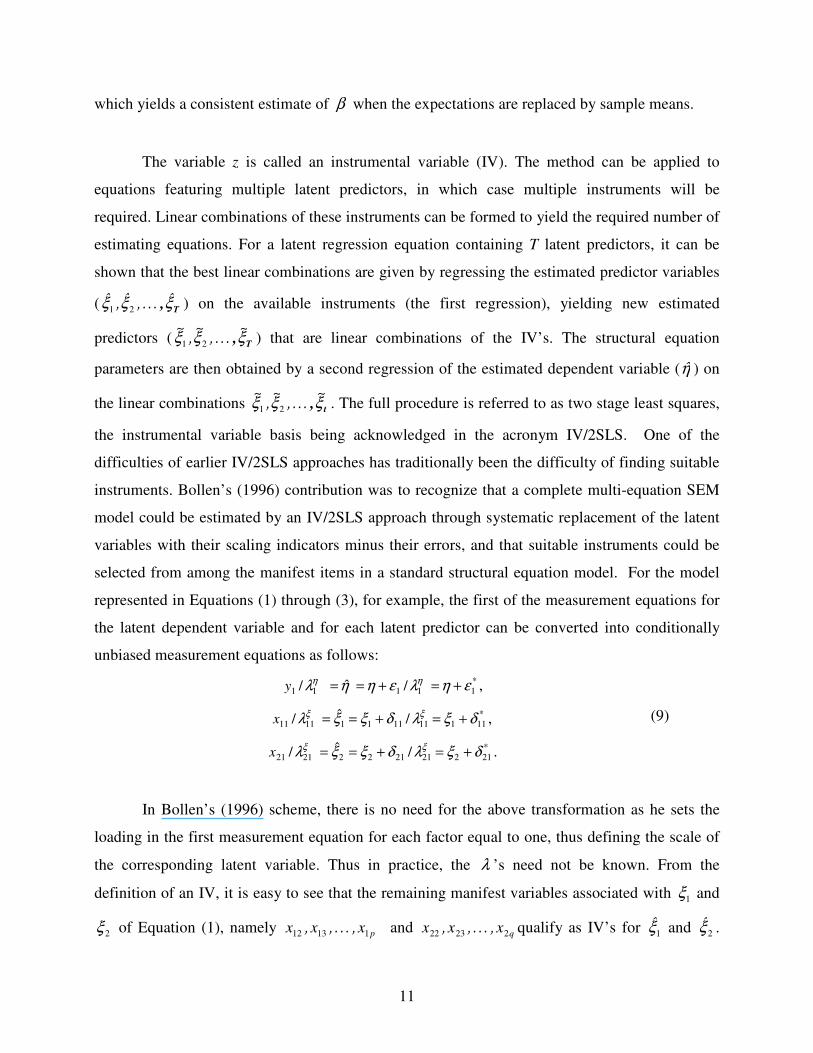
which yields a consistent estimate of β when the expectations are replaced by sample means.

The variable z is called an instrumental variable (IV). The method can be applied to

equations featuring multiple latent predictors, in which case multiple instruments will be

required. Linear combinations of these instruments can be formed to yield the required number of

estimating equations. For a latent regression equation containing T latent predictors, it can be

shown that the best linear combinations are given by regressing the estimated predictor variables

( T, ξξξ ����� 21 ) on the available instruments (the first regression), yielding new estimated

predictors ( T, ξξξ �����

��

�21 ) that are linear combinations of the IV’s. The structural equation

parameters are then obtained by a second regression of the estimated dependent variable (η ) on

the linear combinations t, ξξξ �����

��

�21 . The full procedure is referred to as two stage least squares,

the instrumental variable basis being acknowledged in the acronym IV/2SLS. One of the

difficulties of earlier IV/2SLS approaches has traditionally been the difficulty of finding suitable

instruments. Bollen’s (1996) contribution was to recognize that a complete multi-equation SEM

model could be estimated by an IV/2SLS approach through systematic replacement of the latent

variables with their scaling indicators minus their errors, and that suitable instruments could be

selected from among the manifest items in a standard structural equation model. For the model

represented in Equations (1) through (3), for example, the first of the measurement equations for

the latent dependent variable and for each latent predictor can be converted into conditionally

unbiased measurement equations as follows:

*11111 /ˆ/ εηλεηηλ ηη +=+== y ,

*1111111111111 /ˆ/ δξλδξξλ ξξ +=+== x , (9)

*2122121222121 /ˆ/ δξλδξξλ ξξ +=+== x .

In Bollen’s (1996) scheme, there is no need for the above transformation as he sets the

loading in the first measurement equation for each factor equal to one, thus defining the scale of

the corresponding latent variable. Thus in practice, the λ ’s need not be known. From the

definition of an IV, it is easy to see that the remaining manifest variables associated with 1ξ and

2ξ of Equation (1), namely pxxx 11312 ������ and qxxx 22322 ������ qualify as IV’s for 1ξ and 2ξ .

12

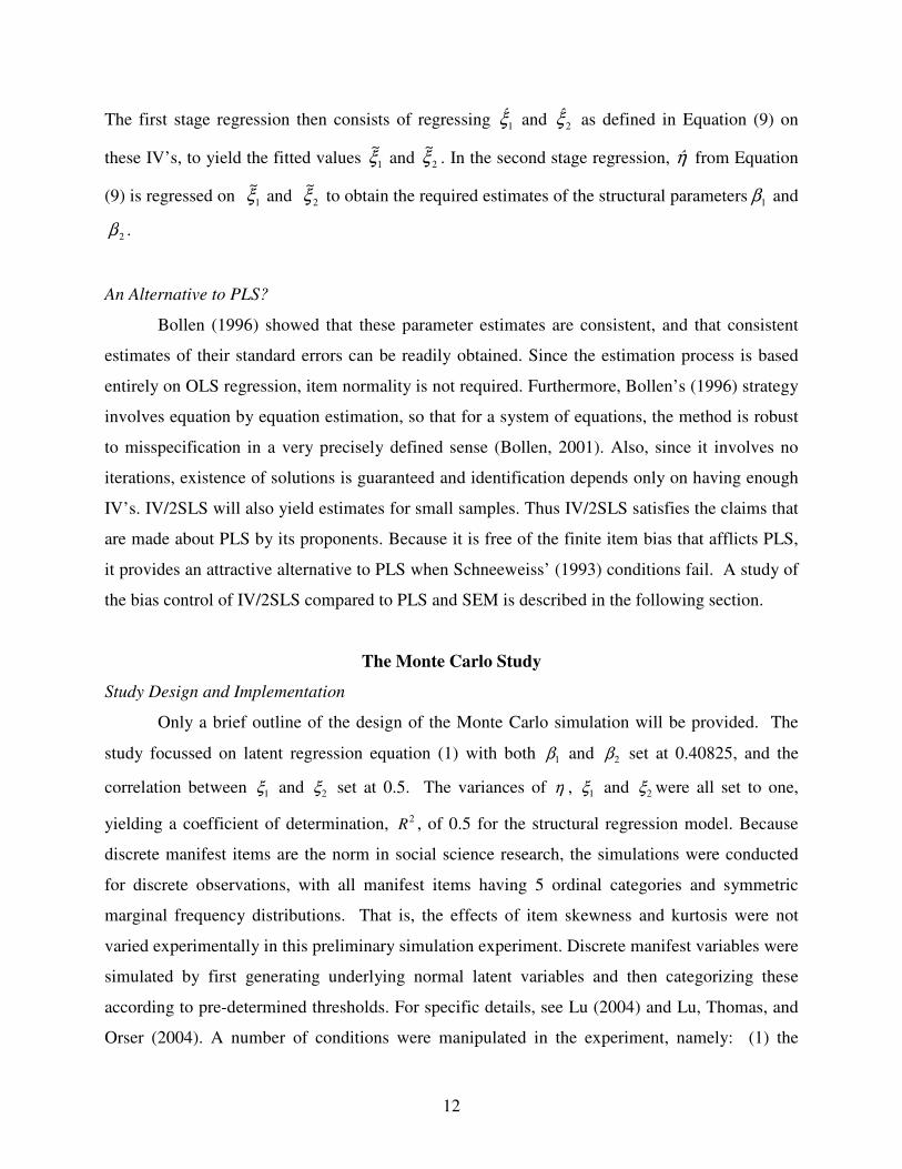
The first stage regression then consists of regressing 1ξ and 2ξ as defined in Equation (9) on

these IV’s, to yield the fitted values 1ξ� and 2ξ� . In the second stage regression, η from Equation

(9) is regressed on 1ξ� and 2ξ� to obtain the required estimates of the structural parameters 1β and

2β .

An Alternative to PLS?

Bollen (1996) showed that these parameter estimates are consistent, and that consistent

estimates of their standard errors can be readily obtained. Since the estimation process is based

entirely on OLS regression, item normality is not required. Furthermore, Bollen’s (1996) strategy

involves equation by equation estimation, so that for a system of equations, the method is robust

to misspecification in a very precisely defined sense (Bollen, 2001). Also, since it involves no

iterations, existence of solutions is guaranteed and identification depends only on having enough

IV’s. IV/2SLS will also yield estimates for small samples. Thus IV/2SLS satisfies the claims that

are made about PLS by its proponents. Because it is free of the finite item bias that afflicts PLS,

it provides an attractive alternative to PLS when Schneeweiss’ (1993) conditions fail. A study of

the bias control of IV/2SLS compared to PLS and SEM is described in the following section.

The Monte Carlo Study

Study Design and Implementation

Only a brief outline of the design of the Monte Carlo simulation will be provided. The

study focussed on latent regression equation (1) with both 1β and 2β set at 0.40825, and the

correlation between 1ξ and 2ξ set at 0.5. The variances of η , 1ξ and 2ξ were all set to one,

yielding a coefficient of determination, 2R , of 0.5 for the structural regression model. Because

discrete manifest items are the norm in social science research, the simulations were conducted

for discrete observations, with all manifest items having 5 ordinal categories and symmetric

marginal frequency distributions. That is, the effects of item skewness and kurtosis were not

varied experimentally in this preliminary simulation experiment. Discrete manifest variables were

simulated by first generating underlying normal latent variables and then categorizing these

according to pre-determined thresholds. For specific details, see Lu (2004) and Lu, Thomas, and

Orser (2004). A number of conditions were manipulated in the experiment, namely: (1) the

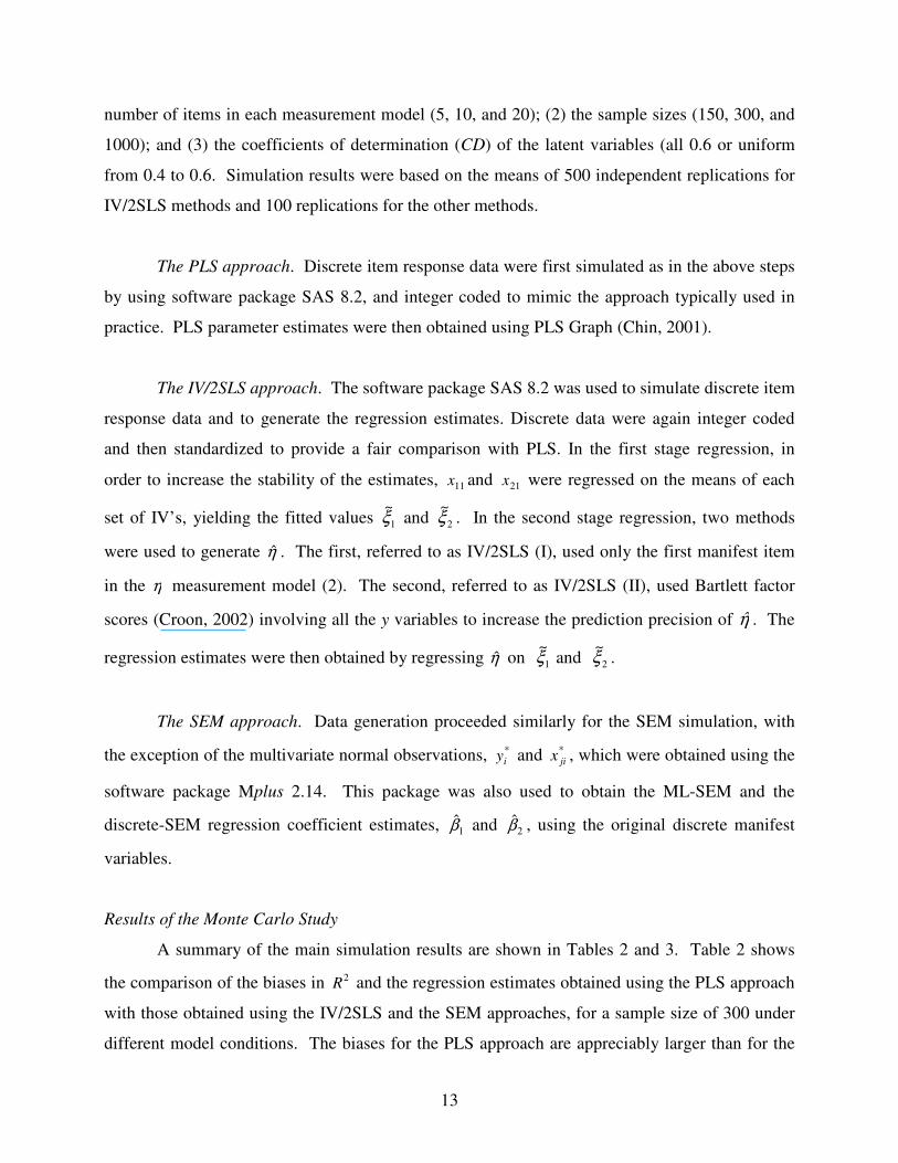
13

number of items in each measurement model (5, 10, and 20); (2) the sample sizes (150, 300, and

1000); and (3) the coefficients of determination (CD) of the latent variables (all 0.6 or uniform

from 0.4 to 0.6. Simulation results were based on the means of 500 independent replications for

IV/2SLS methods and 100 replications for the other methods.

The PLS approach. Discrete item response data were first simulated as in the above steps

by using software package SAS 8.2, and integer coded to mimic the approach typically used in

practice. PLS parameter estimates were then obtained using PLS Graph (Chin, 2001).

The IV/2SLS approach. The software package SAS 8.2 was used to simulate discrete item

response data and to generate the regression estimates. Discrete data were again integer coded

and then standardized to provide a fair comparison with PLS. In the first stage regression, in

order to increase the stability of the estimates, 11x and 21x were regressed on the means of each

set of IV’s, yielding the fitted values 1ξ� and 2ξ� . In the second stage regression, two methods

were used to generate η̂ . The first, referred to as IV/2SLS (I), used only the first manifest item

in the η measurement model (2). The second, referred to as IV/2SLS (II), used Bartlett factor

scores (Croon, 2002) involving all the y variables to increase the prediction precision of η . The

regression estimates were then obtained by regressing η̂ on 1ξ� and 2ξ� .

The SEM approach. Data generation proceeded similarly for the SEM simulation, with

the exception of the multivariate normal observations, *iy and *

jix , which were obtained using the

software package Mplus 2.14. This package was also used to obtain the ML-SEM and the

discrete-SEM regression coefficient estimates, 1β̂ and 2β̂ , using the original discrete manifest

variables.

Results of the Monte Carlo Study

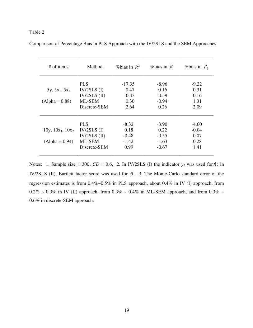
A summary of the main simulation results are shown in Tables 2 and 3. Table 2 shows

the comparison of the biases in 2R and the regression estimates obtained using the PLS approach

with those obtained using the IV/2SLS and the SEM approaches, for a sample size of 300 under

different model conditions. The biases for the PLS approach are appreciably larger than for the

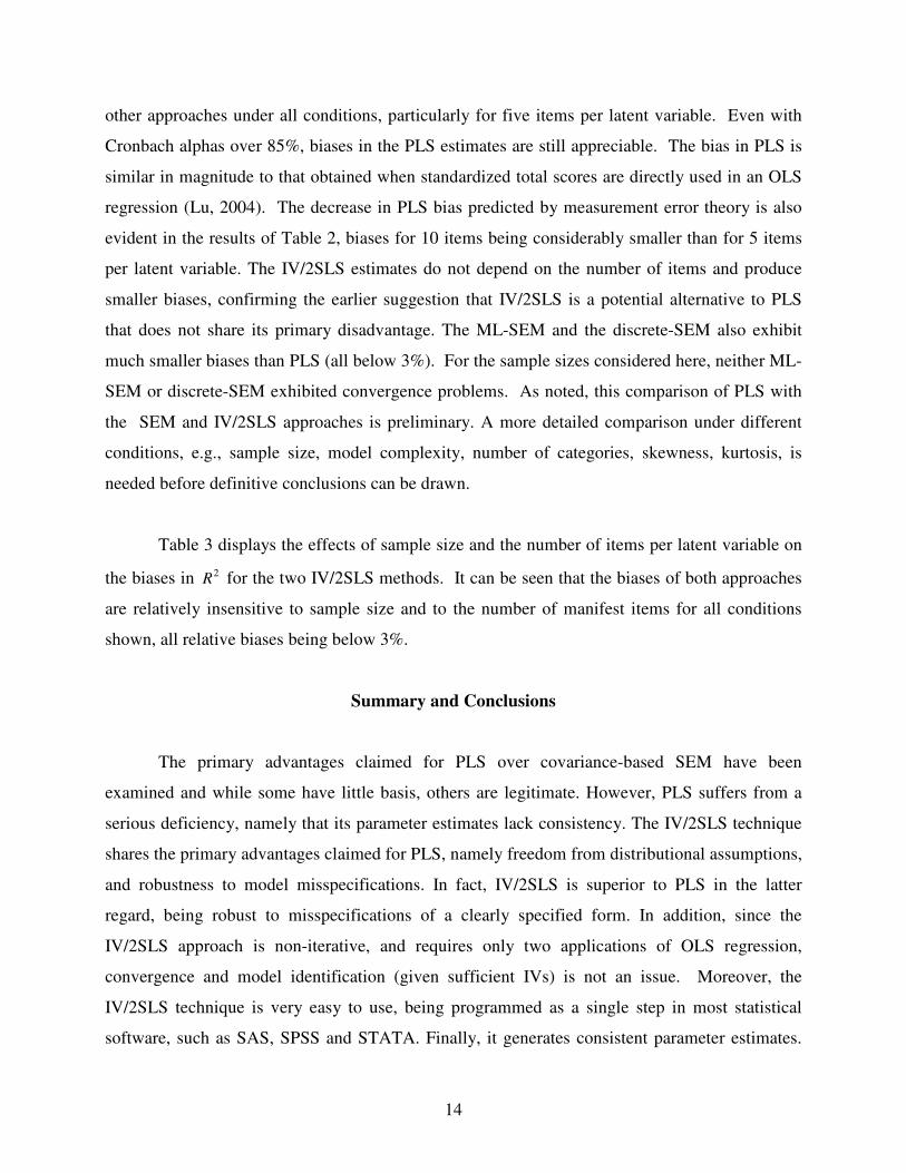
14

other approaches under all conditions, particularly for five items per latent variable. Even with

Cronbach alphas over 85%, biases in the PLS estimates are still appreciable. The bias in PLS is

similar in magnitude to that obtained when standardized total scores are directly used in an OLS

regression (Lu, 2004). The decrease in PLS bias predicted by measurement error theory is also

evident in the results of Table 2, biases for 10 items being considerably smaller than for 5 items

per latent variable. The IV/2SLS estimates do not depend on the number of items and produce

smaller biases, confirming the earlier suggestion that IV/2SLS is a potential alternative to PLS

that does not share its primary disadvantage. The ML-SEM and the discrete-SEM also exhibit

much smaller biases than PLS (all below 3%). For the sample sizes considered here, neither ML-

SEM or discrete-SEM exhibited convergence problems. As noted, this comparison of PLS with

the SEM and IV/2SLS approaches is preliminary. A more detailed comparison under different

conditions, e.g., sample size, model complexity, number of categories, skewness, kurtosis, is

needed before definitive conclusions can be drawn.

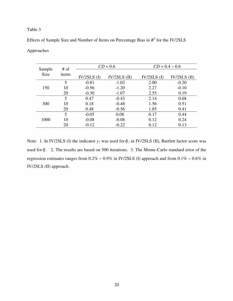
Table 3 displays the effects of sample size and the number of items per latent variable on

the biases in 2R for the two IV/2SLS methods. It can be seen that the biases of both approaches

are relatively insensitive to sample size and to the number of manifest items for all conditions

shown, all relative biases being below 3%.

Summary and Conclusions

The primary advantages claimed for PLS over covariance-based SEM have been

examined and while some have little basis, others are legitimate. However, PLS suffers from a

serious deficiency, namely that its parameter estimates lack consistency. The IV/2SLS technique

shares the primary advantages claimed for PLS, namely freedom from distributional assumptions,

and robustness to model misspecifications. In fact, IV/2SLS is superior to PLS in the latter

regard, being robust to misspecifications of a clearly specified form. In addition, since the

IV/2SLS approach is non-iterative, and requires only two applications of OLS regression,

convergence and model identification (given sufficient IVs) is not an issue. Moreover, the

IV/2SLS technique is very easy to use, being programmed as a single step in most statistical

software, such as SAS, SPSS and STATA. Finally, it generates consistent parameter estimates.

15

Preliminary simulation results confirm that finite item bias in PLS parameter estimates can be

serious, and that IV/2SLS is a potential alternative to PLS that is free of this problem. However,

further studies are required before definitive recommendations can be made.

References

Arminger, G., & Schoenberg, R. J. (1989). Pseudo-maximum likelihood estimation and a test for misspecification in mean and covariance structure models. Psychometrika, 54, 409-425.

Barclay, D. W., Higgins, C., & Thompson, R. (1995). The partial least squares (PLS) approach to causal modeling: Personal computer adaptation and use as an illustration. Technology Studies, 2(2), 285-309.

Bentler, P. M. (1982). Confirmatory factor analysis via noniterative estimation: A fast, inexpensive method. Journal of Marketing Research, 19, 417-424.

Bollen, K. A. (1996). An alternative two stage least squares (2SLS) estimator for latent variable equations. Psychometrika, 61, 109-121.

Bollen, K. A. (2001). Two-stage least squares and latent variable models: Simultaneous estimation and robustness to misspecifications. In R. Cudeck, S. Du Toit , & D. Sörbom (Eds.), Structural equation modeling: Present and future (pp. 119-138). Lincolnswood, IL: Scientific Software.

Bollen, K. A. (2002). Latent variables in psychology and the social sciences. Annual Review of Psychology, 53, 605-634.

Bollen, K. A., & Stine, R. A. (1990). Direct and Indirect effects: Classical and bootstrap estimates of variability. In C. C. Clogg (Ed.), Sociological methodology (pp. 115-140). Oxford: Basil Blackwell.

Boomsma, A. (1983). On the robustness of LISREL (maximum likelihood estimation) against small sample size and nonnormality. Amsterdam: Sociometric Research Foundation.

Browne, M.W. (1984). Asymptotic distribution free methods in analysis of covariance structures. British Journal of Mathematical and Statistical Psychology, 37, 62-83.

Chin, W.W. (1995). Partial least squares is to LISEL as principal components analysis is to factor analysis. Technology Studies, 2, 315-319.

Chin, W.W. (1998). The partial least squares approach to structural equation modeling. In G. A. Marcoulides (Ed.), Modern methods for business research (pp. 295-336). Mahwah, New Jersey: Lawrence Erlbaum Associates.

Chin, W.W. (2001). PLS-graph user’s guide. C.T. Bauer College of Business, University of Houston, USA.

Croon, M. (2002). Using predicted latent scores in general latent structure models. In G. A. Marcoulides & I. Moustaki (Eds.), Latent variable and latent structure models (pp. 195-223). Mahwah, NJ: Lawrence Erlbaum Associates.

Dikstra, T. (1983). Some comments on maximum likelihood and partial least squares methods. Journal of Econometrics, 21, 67-90.

Fuller, W.A. (1987). Measurement error models. New York: Wiley. Gefen, D., Straub, D. W., & Boudreau, M. C. (2000). Structural equation modeling and

regression: Guidelines for research practice. Communications of the Association for Information Systems, 4(7), 1-77.

16

Hanafi, M., & Qannari, E. M. (2005). An alternative algorithm to the PLS B problem. Computational Statistics and Data Analysis, 48, 63-67.

Hoyle, R. H., & Panter, A. T. (1995). Writing about structural equation models. In R. H. Hoyle (Ed.), Structural equation modeling: Concepts, issues, and applications (pp. 158-176). Thousand Oaks, CA: Sage.

Jöreskog, K. G. (1970). A general method for analysis of covariance structures. Biometrika, 57, 239-251.

Jöreskog, K. G., & Sörbom, D. (1996). LISREL 8 user's reference guide. Chicago: Scientific Software International.

Jöreskog, K. G. & Wold, H. (1982). The ML and PLS techniques for modelling with latent variables: Historical and comparative aspects. In K. G. Jöreskog & H. Wold (Eds.), Systems under indirect observation: Causality, structure, prediction (Vol. 1, pp. 263-270). Amsterdam: North-Holland.

Lance, C. E., Cornwell, J. M., & Mulaik, S. A. (1988). Limited information parameter estimates for latent or mixed manifest and latent variable models. Multivariate Behavioral Research, 23, 155-67.

Lu, I. R. R. (2004). Latent variable modeling in business research: A comparison of regression based on IRT and CTT scores with structural equation models. Doctoral dissertation, Carleton University, Canada.

Lu, I. R. R., Thomas, D. R., & Orser, B. J. (2004). Latent variable modeling in business research: A comparison of two-step approach with structural equation modeling. Proceedings of Administrative Sciences Association of Canada, 32nd Annual ASAC Conference, Quebéc city, Quebéc, June 5-8.

Lu, I. R. R., Thomas, D. R., & Zumbo, B. D. (2005). Embedding IRT in structural equation models: A comparison with regression based on IRT scores. Structural Equation Modeling, 12(2), 263-277.

Muthén, B. O. (1984). A general structural equation model with dichotomous, ordered categorical, and continuous latent variable indicators. Psychometrika, 49, 115–132.

Muthén, L. K., & Muthén, B. O. (2001). Mplus user's guide. Los Angeles, CA: Muthén & Muthén.

Muthén, B. O., & Kaplan, D. (1992). A comparison of some methodologies for the factor analysis of non-normal Likert variables: A note on the size of the model. British Journal of Mathematical and Statistical Psychology, 45, 19-30.

Satorra, A. (1992). Asymptotic robust inferences in the analysis of mean and covariance structures. In P. Marsden, (Ed.), Sociological methodology (pp. 249-278). Oxford, England: Blackwell Publishers.

Satorra, A., & Bentler, P. M. (1994). Corrections to test statistics and standard errors in covariance structure analysis. In A. von Eye and C. Clogg (Eds.), Latent variable analysis in developmental research (pp. 285-305). Newbury Park, CA: Sage.

Schneeweiss, H. (1993). Consistency at large in models with latent variables. In K. Haagen, D. J. Bartholomew, & M. Deistler (Eds.), Statistical modelling and latent variables (pp. 299-320). Amsterdam: Elsevier Science Publishers.

Tenenhaus, M., Vinzi, V. E., Chatelin Y-M., & Lauro, C. (2005). PLS path modeling. Computational Statistics and Data Analysis, 48, 159-205.

West, S. G., Finch, J. F., & Curran, P. J. (1995). Structural equation models with nonnormal variables: Problems and remedies. In R. H. Hoyle (Ed.), Structural equation modeling: Concepts, issues, and applications (pp. 56-75). Thousand Oaks, CA: Sage.

17

Wold, H. (1982). Soft modeling: The basic design and some extensions. In K. G. Jöreskog & H. Wold (Eds.), Systems under indirect observation: Causality, structure, prediction (Vol. 2, pp. 1-54). Amsterdam: North-Holland.

Wold, H. (1985). Systems analysis by partial least squares. In P. Nijkamp, H. Leitner, & N. Wrigley (Eds.), Measuring the unmeasurable (pp. 221-251). Boston: Martinus Nijhoff.

Wolins, L. (1995). A Monte-Carlo study of constrained factor-analysis using maximum likelihood and unweighted least-squares. Educational and Psychological Measurement, 55 (4), 545-557.

18

Table 1

Perceived Advantage of PLS Over Covariance-Based SEM

# Claim Counts

1 PLS does not require multivariate normal items. It is distribution free. 11

2 PLS handles formative indicators 7

3 PLS works for small sample sizes 6

4 PLS is better for exploratory studies, and possibly misspecified models 6

5 PLS does not require interval scaled data 6

6 PLS is predictive, as opposed to confirmatory. It minimizes residual error

5

7 PLS does not require independent cases. 5

8 PLS yields consistent or unbiased parameter estimates. 3

9 PLS avoids inadmissible solutions. No convergence or identification problems.

2

10 PLS provides latent variable scores, or case values. 2

19

Table 2

Comparison of Percentage Bias in PLS Approach with the IV/2SLS and the SEM Approaches

# of items

Method

%bias in 2R %bias in 1β�

%bias in 2β�

5y, 5x1, 5x2

(Alpha = 0.88)

PLS IV/2SLS (I) IV/2SLS (II) ML-SEM Discrete-SEM

-17.35 0.47 -0.43 0.30 2.64

-8.96 0.16 -0.59 -0.94 0.26

-9.22 0.31 0.16 1.31 2.09

10y, 10x1, 10x2

(Alpha = 0.94)

PLS IV/2SLS (I) IV/2SLS (II) ML-SEM Discrete-SEM

-8.32 0.18 -0.48 -1.42 0.99

-3.90 0.22 -0.55 -1.63 -0.67

-4.60 -0.04 0.07 0.28 1.41

Notes: 1. Sample size = 300; CD = 0.6. 2. In IV/2SLS (I) the indicator y1 was used forη̂ ; in

IV/2SLS (II), Bartlett factor score was used for η̂ . 3. The Monte-Carlo standard error of the

regression estimates is from 0.4%~0.5% in PLS approach, about 0.4% in IV (I) approach, from

0.2% ~ 0.3% in IV (II) approach, from 0.3% ~ 0.4% in ML-SEM approach, and from 0.3% ~

0.6% in discrete-SEM approach.

20

Table 3

Effects of Sample Size and Number of Items on Percentage Bias in R2 for the IV/2SLS

Approaches

CD = 0.6 CD = 0.4 ~ 0.6 Sample

Size # of

items IV/2SLS (I)

IV/2SLS (II)

IV/2SLS (I)

IV/2SLS (II)

150 5

10 20

-0.81 -0.56 -0.30

-1.02 -1.20 -1.07

2.00 2.27 2.55

-0.20 -0.10

0.19

300 5

10 20

0.47 0.18 0.48

-0.43 -0.48 -0.56

2.14 1.56 1.85

0.68 0.51 0.41

1000 5

10 20

-0.05 -0.08 -0.12

0.08 -0.08 -0.22

0.17 0.12 0.12

0.44 0.24 0.13

Note: 1. In IV/2SLS (I) the indicator y1 was used forη̂ ; in IV/2SLS (II), Bartlett factor score was

used forη̂ . 2. The results are based on 500 iterations. 3. The Monte-Carlo standard error of the

regression estimates ranges from 0.2% ~ 0.9% in IV/2SLS (I) approach and from 0.1% ~ 0.6% in

IV/2SLS (II) approach.