A critical overview of elasto-viscoplastic thixotropic modeling

A critical overview of elasto-viscoplastic thixotropic modeling

Paulo R. de Souza Mendes a,!, Roney L. Thompson b

aDepartment of Mechanical Engineering, Pontifícia Universidade Católica-RJ, Rua Marquês de São Vicente 225, Rio de Janeiro, RJ 22453-900, Brazilb LCFT-LMTA-PGMEC, Department of Mechanical Engineering, Universidade Federal Fluminense, Rua Passo da Pátria 156, Niterói, RJ 24210-240, Brazil

a r t i c l e i n f o

Article history:Received 11 February 2012Received in revised form 8 June 2012Accepted 24 August 2012Available online 2 September 2012

Keywords:ElasticityViscoplasticityThixotropyModeling

a b s t r a c t

The literature on thixotropy modeling is reviewed, with particular emphasis on models for yield stressmaterials that possess elasticity. The various possible approaches that have been adopted to model thedifferent facets of the mechanical behavior of this kind of materials are compared and discussed in detail.An appraisal is given of the advantages and disadvantages of algebraic versus differential stress equa-tions. The thixotropy phenomenon is described as a dynamical system whose equilibrium locus is theflow curve, and the importance of using the flow curve as an input of the model is emphasized. Differentforms for the evolution equation for the structure parameter are analyzed, and appropriate choices areindicated to ensure a truthful description of the thixotropy phenomenon.

! 2012 Elsevier B.V. All rights reserved.

1. General aspects of elasto-viscoplastic thixotropic models

The current status of modeling elasto-viscoplastic thixotropicmaterials has achieved a matured stage, as a result of the develop-ments of important research groups like the ones whose work is ci-ted in this manuscript. Although there is still a long journey aheadto reach the goal of predicting this kind of material behavior undercomplex motion, at least the viscometric response has achieved astage, where a comprehensive critical overview is worth while. Incontrast to the general thixotropic reviews of Mewis [1], Barnes[2], Mujumdar et al.[3], and Mewis and Wagner [4], the presenttext is focused on thixotropic effects in elasto-viscoplastic materi-als. Hence we are particularly interested in identifying in the liter-ature and analyzing the approaches that were employed to modelthe thixotropic behavior combined with elasticity and plasticity.

The various models available in the literature can be roughlygrouped into two different types. In one of these, which we will callType I, the approach starts with a viscoplastic stress equation, towhich elasticity and thixotropy are introduced, following Houska[5] [e.g. 3,6]. In the other type, here denominated Type II, the ap-proach starts with a viscoelastic stress equation, to which plasticityand thixotropy are introduced [e.g. 7,8].

For modeling yield stress materials, in Type II models plasticityis introduced by using a viscosity function that diverges at highstructuring levels [9,7]. For apparent yield stress fluids, a viscosityfunction that possesses a high-viscosity Newtonian plateau in thelow strain-rate limit is employed [10,8,11]. A recent Type II model

has been proposed that accommodates both true yield stress mate-rials and apparent yield stress fluids [12].

The most usual way to model thixotropic behavior is to intro-duce a structure parameter, typically called k, that represents thelevel of organization of the material internal microstructure.

The next step is generally to postulate a correlation between thestructure parameter k and bulk properties such as viscosity andelastic modulus (or yield stress). A common feature of thixotropymodels is to introduce an evolution equation for the structureparameter to capture the time-dependent behavior of the material.This is invariably formatted as a kinetic equation, where the com-petition between a buildup and a breakdown term is represented[13]. An equilibrium or steady state condition is achieved whenthe rates of destruction and of construction of the microstructurebecome equal.

2. Type I models

The Bingham model has a very strong influence on the visco-plasticity literature. Accordingly, a large number of thixotropymodels available in the literature are of Type I, i.e. are based onthe Bingham model, to which other features are added.

The Bingham model clearly arises from the introduction of theyield stress in the classic Newtonian fluid constitutive model.The yield stress sy is an entity that traditionally appears in consti-tutive equations of solid mechanics. When subjected to stress lev-els below this yield stress, the material has a ‘‘solid-like behavior’’,and above the yield stress it possesses a ‘‘liquid-like behavior’’.

In the Bingham model, the solid-like and the liquid-likecontributions are combined as additive parts of the total stress s.

0377-0257/$ - see front matter ! 2012 Elsevier B.V. All rights reserved.http://dx.doi.org/10.1016/j.jnnfm.2012.08.006

! Corresponding author. Tel.: +55 2131141177; fax: +55 2131141165.E-mail addresses: [email protected] (P.R. de Souza Mendes), rthompson@

mec.uff.br (R.L. Thompson).

Journal of Non-Newtonian Fluid Mechanics 187-188 (2012) 8–15

Contents lists available at SciVerse ScienceDirect

Journal of Non-Newtonian Fluid Mechanics

journal homepage: ht tp : / /www.elsevier .com/locate / jnnfm

Therefore, thinking in terms of a mechanical analog, we can saythat the two contributions are combined ‘‘in parallel.’’ An impor-tant consequence of this framework is that the viscosity goes toinfinity as the strain rate approaches zero.

The Newtonian fluid contribution may be replaced by a non-linear function of the strain rate. If this is done, then we get a mod-ified Bingham model that keeps its essential features. For example,if a power-law dependence with the strain rate is assumed, thenthe Herschel–Bulkley model is obtained. The Herschel–Bulkleymodel is perhaps the most representative constitutive relation ofthis kind, and also the most used one.

The solid mechanicians usually assume that below the yieldstress the material presents an elastic behavior, which is most of-ten ignored by the fluid mechanicians when modeling a viscoplas-tic material. However, it is true that a number of fluid-mechanicsoriented authors proposed ways to add elasticity in a Bingham-likemodel.

The most intuitive way to introduce elasticity into a viscoplasticmodel was proposed by Oldroyd [14], by replacing the solid contri-bution, i.e. the behavior below the yield stress, by an expressionthat takes the form of a Hookean solid. Thus, the elastic modulusG—another traditional quantity in solid mechanics—comes intoplay. In this case, the resulting constitutive equation is

s ! sy " lp _c if s P sys ! Gc if s < sy

!#1$

where lp is the plastic viscosity, c is the strain, and _c is the strainrate. Interestingly, this additional elastic expression creates anequivalence between the yield stress and a yield strain, the latterbeing defined as the deformation that occurs at the yield point, gi-ven by cy = sy/G.

Thixotropic models of Type I follow Oldroyd’s general idea tointroduce elasticity into the stress equation. In these models, thefeatures of Eq. (1) are generally expressed in the following singleequation for the stress:

s ! Gsce " gs _c #2$

In this equation, Gs is a structural elastic modulus, gs is a struc-tural viscosity, and ce is the elastic strain, i.e. the recoverable partof the total strain.

Representative elasto-viscoplastic thixotropic models [e.g. 3,6]originate from Oldroyd’s approach described above. Four ingredi-ents compose the models of this type: (i) the equation for stress,(ii) the relation between the material properties and the structureparameter, (iii) the evolution equation for k, and (iv) an equationfor the evolution of elastic strain ce. The three first ingredients alsoappear in Type II models (to be discussed later), while the lastingredient deserves special attention, due to its crucial role in themechanical behavior predicted by Type I models.

The physical reasoning that leads to a specific type of evolutionequation for ce is typically not discussed in enough detail in the lit-erature, in contrast to the prolific discussions often found to de-scribe the underlying physics of the other model ingredients. Forexample, it is common that the evolution equation for the struc-ture parameter be described as a competition between a break-down term and a buildup term. It follows that some generalfeatures arise from this viewpoint which provide guidance to theconstruction of a newmodel. The process of building a specific evo-lution equation for k is thus reduced to deciding what characteris-tic thixotropic time will be used, which parameters should bechosen to appear in the buildup term, what physical quantity isresponsible for the destruction of the material microstructure,and so on, as it will be discussed later on in this text. There areno counterparts, clearly stressed in the literature, for the evolutionequation of ce.

2.1. Examining Type I models from the viewpoint of mechanicalanalogs

It is interesting to analyze Type I models from the mechanical-analog viewpoint. Note that the existence of some mechanical ana-log for every model is a requirement of Newton’s second law.

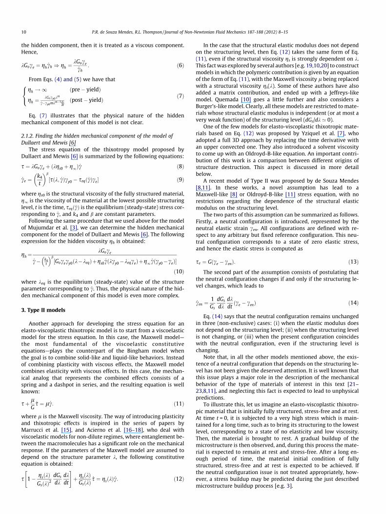
The two additive terms of Eq. (2) imply a mechanical analogwith two branches, one whose stress intensity is g _c, and the otherwhose stress intensity is Gce. Since c % ce, the equation for stresscannot be translated in to a mechanical analog in a straightforwardmanner. There is a need for a description of the mechanism thatrules the deformation c & ce. A possible analog for Type I modelsis shown in Fig. 1. This analog possesses a mechanical componentin series with the elastic component Gce. Because, by definition, theelasticity of the model is given by the elastic component Gce alone,it is reasonable to infer that this component—indicated by an inter-rogation mark in Fig. 1—is a viscous mechanism of the form gh _ch,where _ch ! _c& _ce is its strain rate. The subscript h stands for ‘‘hid-den,’’ because this component does not appear explicitly in theformulation.

The presence of this hidden mechanical component is whatmakes Eq. (2) different from the one describing a Kelvin–Voigtmaterial. This hidden mechanical component governs the strainrate _ch ! _c& _ce. In other words, the evolution equation for ce is di-rectly related to an evolution equation for ch, which in turn is aconsequence of the physical nature of the hidden mechanicalcomponent.

Next we examine two thixotropic models representative ofType I under the optics of the mechanical analog shown in Fig. 1.In these models, like in the vast majority of the models availablein the literature, the structure parameter is defined such that itvaries within the range between 0 and 1; k = 1 indicates the high-est structuring level, while k = 0 corresponds to the lowest struc-turing level.

2.1.1. Finding the hidden mechanical component of the model ofMujumdar et al. [3]

The stress equation of the thixotropy model proposed byMujumdar et al. [3] is summarized below:

s ! kGoce " #1& k$K _cn #3$_ce ! _c if jcej < cy#k$ #pre& yield$jcej ! cy#k$ #post& yield$

(#4$

where cy#k$ ! cy0km #5$

In the equations above, Go is the structural elastic modulus ofthe fully structured material, K is the consistency index, n is thepower-law index, and cy0 is the elastic strain of the fully structuredmaterial.

It is clear that the stress acting at the hidden mechanical com-ponent is the same as the stress acting at the elastic component. Asdiscussed earlier in a general context, since there is no elasticity in

Fig. 1. A possible mechanical analog for Type I models.

P.R. de Souza Mendes, R.L. Thompson / Journal of Non-Newtonian Fluid Mechanics 187-188 (2012) 8–15 9

the hidden component, then it is treated as a viscous component.Hence,

kGoce ! gh _ch ) gh ! kGoce_ch

: #6$

From Eqs. (4) and (5) we have that

gh ! 1 #pre& yield$

gh ! kGocy0km

_c&cy0mkm&1dkdt

#post& yield$

8<

: #7$

Eq. (7) illustrates that the physical nature of the hiddenmechanical component of this model is not clear.

2.1.2. Finding the hidden mechanical component of the model ofDullaert and Mewis [6]

The stress equation of the thixotropy model proposed byDullaert and Mewis [6] is summarized by the following equations:

s ! kGoce " #kgs0 " g1$ _c #8$

_ce !k4t

" #b

's#k; _c$cy0 & seq# _c$ce( #9$

where gs0 is the structural viscosity of the fully structured material,g1 is the viscosity of the material at the lowest possible structuringlevel, t is the time, seq# _c$ is the equilibrium (steady-state) stress cor-responding to _c, and k4 and b are constant parameters.

Following the same procedure that we used above for the modelof Mujumdar et al. [3], we can determine the hidden mechanicalcomponent for the model of Dullaert and Mewis [6]. The followingexpression for the hidden viscosity gh is obtained:

gh !kGoce

_c& k4t

$ %b'Gocecy0#k&keq$"gs0 _c#kcy0&keqce$"g1 _c#cy0&ce$(

#10$

where keq is the equilibrium (steady-state) value of the structureparameter corresponding to _c. Thus, the physical nature of the hid-den mechanical component of this model is even more complex.

3. Type II models

Another approach for developing the stress equation for anelasto-viscoplastic thixotropic model is to start from a viscoelasticmodel for the stress equation. In this case, the Maxwell model—the most fundamental of the viscoelastic constitutiveequations—plays the counterpart of the Bingham model whenthe goal is to combine solid-like and liquid-like behaviors. Insteadof combining plasticity with viscous effects, the Maxwell modelcombines elasticity with viscous effects. In this case, the mechan-ical analog that represents the combined effects consists of aspring and a dashpot in series, and the resulting equation is wellknown:

s" lG_s ! l _c: #11$

where l is the Maxwell viscosity. The way of introducing plasticityand thixotropic effects is inspired in the series of papers byMarrucci et al. [15], and Acierno et al. [16–18], who deal withviscoelastic models for non-dilute regimes, where entanglement be-tween the macromolecules has a significant role on the mechanicalresponse. If the parameters of the Maxwell model are assumed todepend on the structure parameter k, the following constitutiveequation is obtained:

s 1& gs#k$Gs#k$2

dGs

dkdkdt

" #" gs#k$Gs#k$

_s ! gs#k$ _c: #12$

In the case that the structural elastic modulus does not dependon the structuring level, then Eq. (12) takes the same form of Eq.(11), even if the structural viscosity gs is strongly dependent on k.This factwas explored by several authors [e.g. 19,10,20] to constructmodels in which the polymeric contribution is given by an equationof the form of Eq. (11), with the Maxwell viscosity l being replacedwith a structural viscosity gs(k). Some of these authors have alsoadded a matrix contribution, and ended up with a Jeffreys-likemodel. Quemada [10] goes a little further and also considers aBurger’s-likemodel. Clearly, all thesemodels are restricted tomate-rials whose structural elastic modulus is independent (or at most avery weak function) of the structuring level (dGs/dk ’ 0).

One of the few models for elasto-viscoplastic thixotropic mate-rials based on Eq. (12) was proposed by Yziquel et al. [7], whoadopted a full 3D approach by replacing the time derivative withan upper convected one. They also introduced a solvent viscosityto come up with an Oldroyd-B-like equation. An important contri-bution of this work is a comparison between different origins ofstructure destruction. This aspect is discussed in more detailbelow.

A recent model of Type II was proposed by de Souza Mendes[8,11]. In these works, a novel assumption has lead to aMaxwell-like [8] or Oldroyd-B-like [11] stress equation, with norestrictions regarding the dependence of the structural elasticmodulus on the structuring level.

The two parts of this assumption can be summarized as follows.Firstly, a neutral configuration is introduced, represented by theneutral elastic strain cen. All configurations are defined with re-spect to any arbitrary but fixed reference configuration. This neu-tral configuration corresponds to a state of zero elastic stress,and hence the elastic stress is computed as

se ! G#ce & cen$: #13$

The second part of the assumption consists of postulating thatthe neutral configuration changes if and only if the structuring le-vel changes, which leads to

_cen ! 1Gs

dGs

dkdkdt

#ce & cen$ #14$

Eq. (14) says that the neutral configuration remains unchangedin three (non-exclusive) cases: (i) when the elastic modulus doesnot depend on the structuring level; (ii) when the structuring levelis not changing, or (iii) when the present configuration coincideswith the neutral configuration, even if the structuring level ischanging.

Note that, in all the other models mentioned above, the exis-tence of a neutral configuration that depends on the structuring le-vel has not been given the deserved attention. It is well known thatthis issue plays a major role in the description of the mechanicalbehavior of the type of materials of interest in this text [21–23,8,11], and neglecting this fact is expected to lead to unphysicalpredictions.

To illustrate this, let us imagine an elasto-viscoplastic thixotro-pic material that is initially fully structured, stress-free and at rest.At time t = 0, it is subjected to a very high stress which is main-tained for a long time, such as to bring its structuring to the lowestlevel, corresponding to a state of no elasticity and low viscosity.Then, the material is brought to rest. A gradual buildup of themicrostructure is then observed, and, during this process the mate-rial is expected to remain at rest and stress-free. After a long en-ough period of time, the material initial condition of fullystructured, stress-free and at rest is expected to be achieved. Ifthe neutral configuration issue is not treated appropriately, how-ever, a stress buildup may be predicted during the just describedmicrostructure buildup process [e.g. 3].

10 P.R. de Souza Mendes, R.L. Thompson / Journal of Non-Newtonian Fluid Mechanics 187-188 (2012) 8–15

Type II models also require additional equations to relate thestructural viscosity and the structural elastic modulus to the struc-ture parameter, and also an evolution equation for the structureparameter itself. However, Type II models do not need an addi-tional evolution equation or rule for ce, in contrast to Type I mod-els, because this information is already embedded in their stressequation. This additional information is needed by Type I modelsbecause their stress equation does not provide it; it is exactly thisinformation that is needed to fully construct their mechanical ana-log (see Eqs. (7) and (10)).

In conclusion, models of Type II are capable of predicting elasticand thixotropic behavior, and plasticity is readily introduced byexpressing the bulk parameters as functions of the structuring le-vel such that the structural viscosity is unbounded when the mate-rial is fully structured [19,7,12].

4. Comparing the stress equations of Type I and Type II models

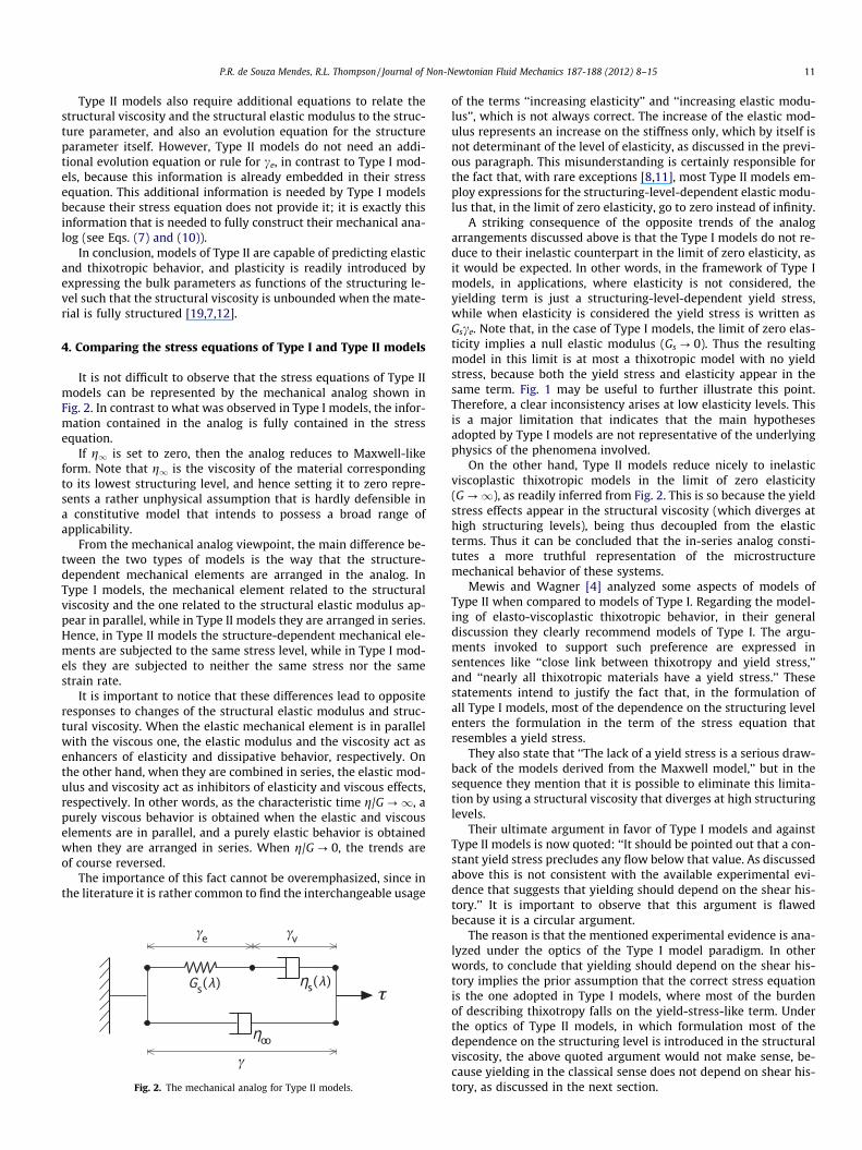
It is not difficult to observe that the stress equations of Type IImodels can be represented by the mechanical analog shown inFig. 2. In contrast to what was observed in Type I models, the infor-mation contained in the analog is fully contained in the stressequation.

If g1 is set to zero, then the analog reduces to Maxwell-likeform. Note that g1 is the viscosity of the material correspondingto its lowest structuring level, and hence setting it to zero repre-sents a rather unphysical assumption that is hardly defensible ina constitutive model that intends to possess a broad range ofapplicability.

From the mechanical analog viewpoint, the main difference be-tween the two types of models is the way that the structure-dependent mechanical elements are arranged in the analog. InType I models, the mechanical element related to the structuralviscosity and the one related to the structural elastic modulus ap-pear in parallel, while in Type II models they are arranged in series.Hence, in Type II models the structure-dependent mechanical ele-ments are subjected to the same stress level, while in Type I mod-els they are subjected to neither the same stress nor the samestrain rate.

It is important to notice that these differences lead to oppositeresponses to changes of the structural elastic modulus and struc-tural viscosity. When the elastic mechanical element is in parallelwith the viscous one, the elastic modulus and the viscosity act asenhancers of elasticity and dissipative behavior, respectively. Onthe other hand, when they are combined in series, the elastic mod-ulus and viscosity act as inhibitors of elasticity and viscous effects,respectively. In other words, as the characteristic time g/G?1, apurely viscous behavior is obtained when the elastic and viscouselements are in parallel, and a purely elastic behavior is obtainedwhen they are arranged in series. When g/G? 0, the trends areof course reversed.

The importance of this fact cannot be overemphasized, since inthe literature it is rather common to find the interchangeable usage

of the terms ‘‘increasing elasticity’’ and ‘‘increasing elastic modu-lus’’, which is not always correct. The increase of the elastic mod-ulus represents an increase on the stiffness only, which by itself isnot determinant of the level of elasticity, as discussed in the previ-ous paragraph. This misunderstanding is certainly responsible forthe fact that, with rare exceptions [8,11], most Type II models em-ploy expressions for the structuring-level-dependent elastic modu-lus that, in the limit of zero elasticity, go to zero instead of infinity.

A striking consequence of the opposite trends of the analogarrangements discussed above is that the Type I models do not re-duce to their inelastic counterpart in the limit of zero elasticity, asit would be expected. In other words, in the framework of Type Imodels, in applications, where elasticity is not considered, theyielding term is just a structuring-level-dependent yield stress,while when elasticity is considered the yield stress is written asGsce. Note that, in the case of Type I models, the limit of zero elas-ticity implies a null elastic modulus (Gs ? 0). Thus the resultingmodel in this limit is at most a thixotropic model with no yieldstress, because both the yield stress and elasticity appear in thesame term. Fig. 1 may be useful to further illustrate this point.Therefore, a clear inconsistency arises at low elasticity levels. Thisis a major limitation that indicates that the main hypothesesadopted by Type I models are not representative of the underlyingphysics of the phenomena involved.

On the other hand, Type II models reduce nicely to inelasticviscoplastic thixotropic models in the limit of zero elasticity(G?1), as readily inferred from Fig. 2. This is so because the yieldstress effects appear in the structural viscosity (which diverges athigh structuring levels), being thus decoupled from the elasticterms. Thus it can be concluded that the in-series analog consti-tutes a more truthful representation of the microstructuremechanical behavior of these systems.

Mewis and Wagner [4] analyzed some aspects of models ofType II when compared to models of Type I. Regarding the model-ing of elasto-viscoplastic thixotropic behavior, in their generaldiscussion they clearly recommend models of Type I. The argu-ments invoked to support such preference are expressed insentences like ‘‘close link between thixotropy and yield stress,’’and ‘‘nearly all thixotropic materials have a yield stress.’’ Thesestatements intend to justify the fact that, in the formulation ofall Type I models, most of the dependence on the structuring levelenters the formulation in the term of the stress equation thatresembles a yield stress.

They also state that ‘‘The lack of a yield stress is a serious draw-back of the models derived from the Maxwell model,’’ but in thesequence they mention that it is possible to eliminate this limita-tion by using a structural viscosity that diverges at high structuringlevels.

Their ultimate argument in favor of Type I models and againstType II models is now quoted: ‘‘It should be pointed out that a con-stant yield stress precludes any flow below that value. As discussedabove this is not consistent with the available experimental evi-dence that suggests that yielding should depend on the shear his-tory.’’ It is important to observe that this argument is flawedbecause it is a circular argument.

The reason is that the mentioned experimental evidence is ana-lyzed under the optics of the Type I model paradigm. In otherwords, to conclude that yielding should depend on the shear his-tory implies the prior assumption that the correct stress equationis the one adopted in Type I models, where most of the burdenof describing thixotropy falls on the yield-stress-like term. Underthe optics of Type II models, in which formulation most of thedependence on the structuring level is introduced in the structuralviscosity, the above quoted argument would not make sense, be-cause yielding in the classical sense does not depend on shear his-tory, as discussed in the next section.Fig. 2. The mechanical analog for Type II models.

P.R. de Souza Mendes, R.L. Thompson / Journal of Non-Newtonian Fluid Mechanics 187-188 (2012) 8–15 11

5. Comments on yielding

The yield stress sy was firstly introduced as a steady-state flowconcept, being defined as the stress below which no unrecoverabledeformation is observed. It is thus a single fixed parameter of theflow curve, and below the yield stress there is no steady state flow( _c ! 0 in the flow curve). It is simply given bysy ! limt!1'lim _c!0s# _c; t$(. The yield stress is also the minimumstress required to trigger a major microstructure breakdown inan initially fully-structured material. It is thus a quantity relatedto the fully structured state only.

Hence, to use the term yield stress to denote a quantity that is afunction of the structuring level is clearly not consistent with theconcept of yield stress. This inconsistency is commented by Mewisand Wagner [4]: ‘‘It could be argued on physical grounds thatattributing a Bingham yield stress to a structure that exists duringflow is not suitable. In practice it is often found to be adequateparameter to fit constant k curves.’’

As discussed earlier, the strategy usually employed by the mostrepresentative Type I models in order to incorporate thixotropy ef-fects is to modify a classical flow curve expression by introducingthe dependence on the structure parameter. Taking the Herschel–Bulkley equation as an example, the idea is to allow the flow curveparameters to depend on the structuring level:

s ! sy#k$ " K#k$ _cn#k$ #15$

It is worth noting that, in most applications that use this type ofequation [e.g. 24], K and n are taken as constants, so that thedependence on the structuring level appears in the first RHS term(sy(k)) only.

The underlying physics of Eq. (15) is not clear. Due to the histor-ical use of the symbol sy in association with the yield stress, one isreadily invited to interpret sy(k) as a yield stress that depends onthe structure parameter. And in fact this is the usual interpretationin a vast majority of articles. However, while the classic Herschel–Bulkley equation represents a flow curve, Eq. (15) does not. Actu-ally, Eq. (15) represents a family of curves parametrized by k (seeBarnes [2] and Fig. 4 therein).

The flow curve is the relation between stress (or viscosity)and strain rate that is observed in steady flow. Each point ofthe flow curve is associated with a different value of k, i.e. a dif-ferent structuring level. Therefore, the flow curve is interceptedby each and every curve obtained from equations of the typeof Eq. (15). This means that, if an equation such as Eq. (15) isemployed, then there will be a different value of sy(k) associatedwith each point of the flow curve, even in the range of very highstrain rates. While the material is flowing, no yielding process—i.e. dramatic change in the microstructure—occurs that couldpossibly justify interpreting sy(k) as a yield stress. Therefore itbecomes quite clear that the only resemblance between sy(k)and the concept of yield stress originates from the form ofEq. (15).

It is worth emphasizing that the discussion above is directed to-wards physical meaning and nomenclature issues only. There is noimplication regarding the appropriateness of employing stressequations of the form of Eq. (15). A straightforward way to pre-serve the concept of yield stress and to preclude further nomencla-ture confusions is to use different symbols to denote the structuredependent parameter in Eq. (15):

s#k; _c$ ! A#k$ " B#k$ _cC#k$: #16$

The parameter A(k) is given by A#k$ ! lim _c!0s#k; _c$, and itshould be seen just as a convenient quantity for fitting constant kcurves, as suggested by Mewis and Wagner [4].

As a final comment on equations of the type of Eq. (15)—which,as mentioned above, originate from the classic Herschel–Bulkleyflow curve—it is interesting to observe that the flow curve corre-sponding to these equations is not the Herschel–Bulkley one, inas-much as sy, K, and n will be functions of the shear rate:

s ! sy#keq# _c$$ " K#keq# _c$$ _cn#keq# _c$$ #17$

where keq# _c$ is the structural parameter under equilibrium (steady-state) conditions (see Eq. (19) below for an example of keq# _c$). Con-sequently, the thixotropy models that employ stress equations likeEq. (15) do not reduce to the Herschel–Bulkley equation as thixot-ropy becomes negligible. This important fact is not discussed inthe literature, and, actually, flow curve equations are seldom givenexplicitly.

6. The role of the flow curve in thixotropy modeling

6.1. General aspects

Some theories for predicting the behavior of microstructuredliquids are developed with basis on features of the microstructureand its interactions with the main flow. Other theories are basedon mechanical analogs.

The resulting model is then checked with respect to its ability topredict the trends observed experimentally in different flow situa-tions, including steady shear flow and other rheological flows. Ifthe trends are correct, then the model parameters can in principlebe determined, acquiring the status of properties of the material.

In the case of thixotropy modeling, an alternate approach fordeveloping a constitutive theory is to use the flow curve as an in-put for the model [8,11]. Since this curve can in principle be ob-tained in laboratory, it is a material property that containsvaluable information about the material behavior in shear, beinganalogous to the viscosity of the Newtonian fluids. Hence, to usethis information in the construction of the model seems to be anatural choice.

A similar approach was used by Schunk and Scriven [25] andothers [e.g. 26–30] in the context of predicting viscoelastic behav-ior in complex flows.

One immediate advantage of this approach is the obvious factthat the flow curve is predicted exactly. Other advantages are dis-cussed in detail in the following sections. It will be shown that theimportance and convenience of using the flow curve as an input fora thixotropy model cannot be overemphasized.

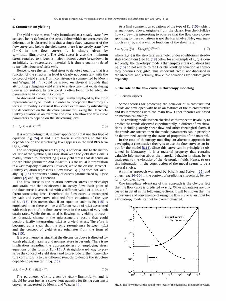
Fig. 3. The flow curve as the equilibrium locus of the dynamical thixotropic system.

12 P.R. de Souza Mendes, R.L. Thompson / Journal of Non-Newtonian Fluid Mechanics 187-188 (2012) 8–15

6.2. The flow curve as the set of all attractor points

The flow curve is the equilibrium locus of the dynamical thixo-tropic system. Therefore, the evolution equation for the structureparameter must be such that these equilibrium points are reach-able and linearly stable.

Considering viscometric flows, the flow curve is thus the set ofattractor points of non-equilibrium states on the Cartesian plane_c) s. In other words, if at some instant of time t0 the point# _ct0 ; st0 $ on this plane does not belong to the flow curve (Fig. 3),then it represents a non-equilibrium state of the microstructure,and hence there is a potential that drives this point along a trajec-tory that ends at some point on the flow curve.

Therefore, it becomes clear that introducing the flow curve asinput into the thixotropy model defines a priori the correct locusof atractor points, which constitutes a piece of information thatis crucial to the predictive capability of the model.

It remains to determine which point on the flow curve is theattractor point for the current state. This issue is not as straight-forward as it may seem at first glance. For example, in a constantstrain rate experiment, the steady-state situation which corre-sponds to the current state is defined by the intersection betweenthe vertical line of the current strain rate and the flow curve. Onthe other hand, in a constant stress experiment the steady-statepoint corresponding to the current state is defined by the inter-section between the horizontal line of the current stress andthe flow curve. In these two flows, it may appear that this stea-dy-state point is the only attractor point throughout the flow,but it may be not.

As it is explained in the following section, in fact the attractorpoint is defined by the characteristics of the evolution equationfor the structure parameter used by the model. Therefore, thesecharacteristics must bear the correct physics, under penalty ofunrealistic predictions.

6.3. The implicit choice of the attractor point

We now analyze a typical kinetic equation whose form is repre-sentative of several evolution equations for the structure parame-ter found in the literature, for the case that k is chosen to varybetween 0 (fully unstructured state) and 1 (fully structured state).This typical equation is written as

dkdt

! 1teq

'k1#1& k$ & k2kg# _c$(; #18$

where teq, k1 and k2 are non-negative constants and g# _c$ is a non-negative function of the strain rate. Eq. (18) assumes that the build-up term is proportional to the ‘‘distance’’ (1 & k) from the present tothe fully structured state, and that the breakdown term is propor-tional both to the ‘‘distance’’ (k & 0) from the present to the fullyunstructured state and to a function of the strain rate, g# _c$. Theequilibrium (steady-state) value of the structure parameter, keq isgiven by

keq# _c$ !k1

k1 " k2g# _c$#19$

keq# _c$ is the value of the structure parameter corresponding to theflow curve at the strain rate _c.

It is observed that the equilibrium states as given by Eq. (19) arelinearly stable, since, for a small departure from the equilibriumstate Dk, the corresponding derivative of k acquires the sign thatwill drive k back to its equilibrium value:

dkdt

! & k1 " k2g# _c$teq

Dk; #20$

For evolution equations like Eq. (18), which possess a break-down term that is a function of the strain rate, it is seen that thekeq value that is the attractor point for the (non-equilibrium) valueof k at time t depends on the value of the strain rate at the sametime t, say _ct .

This is better understood with the aid of Fig. 3, where we cansee that a constant strain rate experiment starting at time t = t0is a vertical trajectory _c ! _ct0 on the _c) s plane. During the exper-iment, both the function g# _c$ and the equilibrium structure param-eter keq remain fixed at g# _ct0 $ and k1='k1 " k2g# _ct0 $(, respectively.

The point of the flow curve that plays the role of the attractor ofthe dynamical system is a fixed point corresponding to the pair# _ct0 ; s# _ct0 $$, where the function s# _c$ gives the value of s of the(steady-state) flow curve corresponding to _c.

A constant shear stress experiment starting at time t = t0 wouldlead to a horizontal trajectory s ! st0 on the _c) s plane. However,due to the dependence of the function g on _c, the equilibrium struc-ture parameter keq is not constant. Since keq is a function of the cur-rent value of the strain rate, this quantity varies along the constantstress trajectory. Therefore, the attractor point on the flow curvealso changes with time. At the current time t, it corresponds tothe point # _ct ; s# _ct$$ on the flow curve, where _ct0 6 _ct 6 s&1#st0 $,and the function s&1(s) is the inverse function of s# _c$, i.e. it givesthe value of _c on the flow curve corresponding to s.

In summary, equations such as Eq. (18) implicitly assume thatthe changes of structuring level are dictated by the strain rate.

A totally different response is obtained if instead we employ thefollowing form of evolution equation for k:

dkdt

! 1teq

'c1#1& k$ & c2kf #s$( ) keq#s$ !c1

c1 " c2f #s$; #21$

where teq, c1 and c2 are non-negative constants and f(s) is a non-negative function of the stress. An equation similar to Eq. (21)was proposed by De Kee and Fong [9], for a kinetic equation forthe number of structural bonds.

For evolution equations like Eq. (21), in a constant strain rateexperiment ( _c ! _ct0 ) starting at t = t0, the attractor point on theflow curve changes with time, while in a constant stress experi-ment (s ! st0 ) starting at t = t0, the atractor point is fixed, corre-sponding to keq#st0 $. Therefore, equations such as Eq. (21)implicitly assume that the changes of structuring level are dictatedby the stress.

It is thus clear that these two possible kinds of evolution equa-tion lead to totally different predictions for the dynamic behaviorof the thixotropic system. The recognition of this fact has not re-ceived the deserved attention and is not an issue commonly dis-cussed in the literature of thixotropy. A notable exception isfound in Yziquel et al. [7], where three possible causes of structuredestruction are analyzed: the level of strain rate, the first invariantof the stress, and the level of dissipation. Comparing with experi-mental results, they conclude that the assumption that dissipationis the main cause of breakdown was the better choice. Howeverthey did not test the level of stress (represented by the secondinvariant of the stress tensor).

In the next section we discuss the underlying physics of the twooptions, namely to assume that breaking of the microstructure isgoverned by the stress or by the strain rate.

Before concluding this section, however, we describe how touse the flow curve as an input of the thixotropic model, irrespec-tive of the type chosen for the evolution equation or for the stressequation (Type I or Type II).

Because the structural viscosity is given as a function of k (oneof the assumptions needed in any model), then, if we apply thisfunction to the equilibrium state and invert it, then we obtain keq

P.R. de Souza Mendes, R.L. Thompson / Journal of Non-Newtonian Fluid Mechanics 187-188 (2012) 8–15 13

as a function of the equilibrium structural viscosity, which is givenby the flow curve.

The function g# _c$ (or the function f(s), depending on the type ofthe evolution equation) is readily determined by writing it as afunction of the equilibrium structure parameter keq. Then it canbe eliminated in the evolution equation in favor of keq:

g# _c$ ! k1k2

1& keq# _c$keq# _c$

) dkdt

! k1teq

#1& k$ & k1& keq# _c$keq# _c$

& '#22$

or

f #s$ ! c1c2

1& keq#s$keq#s$

) dkdt

! c1teq

#1& k$ & k1& keq#s$keq#s$

& '#23$

Note that this procedure reduces by one the number of con-stants of the model (k2 and c2 cancel out), and embeds in the for-mulation the correct attractor points of the dynamic thixotropicsystem by using the flow curve to determine keq.

This procedure, firstly proposed by de Souza Mendes [8], seemsmore reasonable than the usual approach, which consists of arbi-trarily guessing a function g# _c$ (or f(s)) and then obtaining a keqwhich will be a direct function of this arbitrary guess. The resultingthixotropy model is usually unable to give acceptable predictionsnot even for the flow curve, and, more important, the thixotropicdynamical system is governed by incorrect driving potentials.

6.4. What breaks the microstructure, is it the strain rate or the stress?

In the previous section we showed that Eqs. (18) and (21) rep-resent rather different descriptions of the evolution of the thixotro-pic dynamical system. Therefore, it is important to decide what isthe choice that gives the best description of the physics involved.

In what follows we argue that it seems much more physicallysound to assume that breaking of the microstructure occurs dueto the stress level. This is because the microstructure involvesbonds between structural units, and bonds consist of interparticleforces. Thus, to break a bond it takes some external force, providedby the stress level. On the other hand, there is no physical argu-ment to support the strain rate as the agent that causes bondbreaking. This line of arguments in favor of the stress as the break-ing agent had already been adumbrated by de Souza Mendes[8,11], but the evolution equation for k proposed therein is notquite consistent with this viewpoint. The correct formulation canbe found in de Souza Mendes and Thompson [12].

It is possible to imagine situations in which the stress is zerobut the strain rate is arbitrarily large, and, since there is no stress,no bond breaking can occur. For example, we can imagine a fullystructured material initially stress-free and at rest, to which attime t = 0 a constant shear rate _c is applied. The stress is zero att = 0 and increases linearly with time during the elastic regime, un-til it reaches the yield stress. No breaking of the microstructure isexpected during the elastic regime (by definition of elastic regimeand yield stress).

Since the strain rate is constant in this case, models that assumethat microstructure breakage is due to the strain rate will predictthe highest breaking rate exactly at t = 0 (because k = 1 and g# _c$is constant), when the stress is zero and hence no breaking what-soever can occur. On the other hand, models that assume thatmicrostructure breakage is due to the stress will perform as ex-pected, because the breakdown term will be zero all the way dur-ing the elastic regime (since k = keq = 1 and hence there is nodriving potential).

It is also worth examining the performance of models employ-ing each of the options in the case of a lump of thixotropic elasto-viscoplastic material, initially at rest and fully structured, on an

inclined plane. Coussot et al. [31] report very interesting experi-mental results for a related problem.

Before discussing model predictions, it is worth describing thephysical behavior expected. It is clear that, if the inclination isnot large enough to generate stresses above the yield stress, thenthe material will remain fully structured and at rest forever, by def-inition of yield stress. For a large enough inclination, the stress le-vel in the material is above the yield stress, and hence breakage ofthe microstructure occurs. Therefore, the lump will eventuallystart moving and deforming down the plane. If thixotropy is negli-gible, the flow starts immediately, while, if not, there will be a de-lay between the moment that the inclination is applied and themoment that the structuring level becomes low enough to causethe viscosity to decrease dramatically, which in turn causes a sud-den flow to take place—the avalanche effect.

Since the initial strain rate is zero in this case (neglecting elas-ticity), models that assume that microstructure breakage is due tothe strain rate will predict no breakage1 of the microstructure,meaning that the lump is predicted to remain at rest and fully struc-tured forever, regardless of the level of stress! On the other hand, mod-els that assume that microstructure breakage is due to the stress willperform as expected. The breakdown term will be zero while in theelastic regime, and will be an increasing function of the stress in thecase that the stress level is above the yield stress. Moreover, the ava-lanche effect is nicely predicted, the delay time being determined byboth the stress level and the equilibrium time teq.

It is also important to emphasize that, even when elasticity ef-fects are not present, it is important to assume that the breakdownterm is a function of the stress rather than the strain rate, as dis-cussed next.

To illustrate this, it is worth analyzing the Lagrangian motion ofa material particle that occupies a given position in a given instantof time, in a complex flow of an inelastic thixotropic yield-stressmaterial. If at this instant of time the material particle is fullystructured (k = 1), then its instantaneous strain rate must be zero(because zero elasticity is assumed). If the breaking agent is chosento be the strain rate, then the breakdown term will always be null.This means that the microstructure of this material particle is pre-dicted to never break, regardless the level of stress to which it is ex-posed. Of course this is unacceptable. On the other hand, it is clearthat the correct prediction is again obtained when the breakdownterm is assumed to be a function of the instantaneous local stress.

Finally it is observed that the two choices for the breaking agentdiscussed above become equivalent in the particular case of yield-stress materials that possess no thixotropy (teq = 0), because k is al-ways equal to keq in this case. In this connection, it is interesting toobserve that, in this limit of no thixotropy, Type II models reduce toelasto-viscoplastic models that look like Maxwell or Jeffreys mod-els, with the structural elastic modulus and structural viscositybeing functions of the equilibrium structure parameter keq. Theresulting models are thus aligned with the standard formulationused to represent this type of behavior. On the other hand, in thesame limit of teq = 0 (no thixotropy), Type I models reduce to mod-els that have no resemblance with the usual formulations, andwhose physical interpretation is not quite clear.

7. Final remarks

In this paper the different aspects involved in elasto-viscoplastic thixotropic models are discussed in detail.

To describe thixotropy, most models rely on the introduction ofa structure parameter, which is a measure of the structuring level

1 Here and in the remainder of this text it is assumed that the function g# _c$appearing as a factor in the breakdown term is null when _c ! 0, as it is invariablypostulated.

14 P.R. de Souza Mendes, R.L. Thompson / Journal of Non-Newtonian Fluid Mechanics 187-188 (2012) 8–15

of the microstructure. This structure parameter is governed by anevolution equation that associates the rate of change of the struc-turing level with a competition between the processes of buildupand breakdown of the microstructure.

In addition to the evolution equation for the structure parame-ter, all models possess a stress equation and expressions that relatethe structural elastic modulus and the structural viscosity with thestructuring level.

If the stress equation is algebraic and originated from theBingham model (Type I models), then an additional equation isneeded to describe the elastic strain ce. For models whose stressequations are differential and originate from the classic viscoelasticmodels (Type II models), no additional equation is needed.

It is argued that the framework of Type II models is more robust,because

* the underlying physics of Type II models are clearly describedby a mechanical analog, and thus the elastic strain ce—a variablepertaining to the microscopic description only—does not appearexplicitly in the formulation;

* Type II models can be seen as general models that reduce nicelyto usual formulations for a wide range of special cases of inter-est, such as inelastic thixotropic viscoplastic materials, and sev-eral types of non-thixotropic materials like elasto-viscoplasticmaterials, and viscoelastic solids and fluids;

* The formulation adopted by Type II models is consistent withthe yield stress concept in its classical sense.

The thixotropy phenomenon is described as a dynamic systemwhose equilibrium locus is the flow curve, and the importance ofusing the flow curve as an input of the model is explained in detail.

Lastly, it is shown that the breakdown term of the evolutionequation for the structure parameter must be a function of theinstantaneous stress (rather than strain rate), under penalty of anunphysical description of the thixotropy phenomenon.

Acknowledgments

The authors are indebted to Petrobras S.A., MCTI/CNPq, CAPES,FAPERJ, and FINEP for the financial support to the Group of Rheol-ogy at PUC-RIO.

References

[1] J. Mewis, Thixotropy—a general review, J. Non-Newtonian Fluid Mech. 6 (1979)1–20.

[2] H.A. Barnes, Thixotropy—a review, J. Non-Newtonian Fluid Mech. 70 (1997) 1–33.

[3] A. Mujumdar, A.N. Beris, A.B. Metzner, Transient phenomena in thixotropicsystems, J. Non-Newtonian Fluid Mech. 102 (2002) 157–178.

[4] J. Mewis, N.J. Wagner, Thixotropy, Adv. Colloid Interface Sci. 147-148 (2009)214–227.

[5] M. Houska, Engineering Aspects of the Rheology of Thixotropic Liquids, Ph.D.Thesis, Czech Technical University of Prague-CVUT, Prague, Czechoslovakia,1981.

[6] K. Dullaert, J. Mewis, A structural kinetics model for thixotropy, J. Non-Newtonian Fluid Mech. 139 (2006) 21–30.

[7] F. Yziquel, P. Carreau, M. Moan, P. Tanguy, Rheological modeling ofconcentrated colloidal suspensions, J. Non-Newtonian Fluid Mech. 86 (1999)133–155.

[8] P.R. de Souza Mendes, Modeling the thixotropic behavior of structured fluids, J.Non-Newtonian Fluid Mech. 164 (2009) 66–75.

[9] D. De Kee, C. Fong, Letter to the editor: a true yield stress?, J Rheol. 37 (1993)775.

[10] D. Quemada, Rheological modelling of complex fluids: IV: Thixotropic and‘‘thixoelastic’’ behaviour. Start-up and stress relaxation, creep tests andhysteresis cycles, Eur. Phys. J. AP 5 (1999) 191–207.

[11] P.R. de Souza Mendes, Thixotropic elasto-viscoplastic model for structuredfluids, Soft Matter 7 (2011) 2471–2483.

[12] P.R. de Souza Mendes, R.L. Thompson, A unified approach to model elasto-viscoplastic thixotropic yield-stress materials and apparent-yield-stress fluids,Rheol. Acta. submitted for publication.

[13] F. Moore, The rheology of ceramic slips and bodies, Trans. Brit. Ceram. Soc. 58(1959) 470–492.

[14] J.G. Oldroyd, A rational formulation of the equations of plastic flow for aBingham solid, Proc. Cambridge Philos. Soc. 43 (1947) 100–105.

[15] G. Marrucci, G. Titomanlio, G.C. Sarti, Testing of a constitutive equationforentangled networks by elongational and shear data of polymer melts, Rheol.Acta 12 (1973) 269–275.

[16] D. Acierno, F.P. La Mantia, G. Marrucci, G. Titomanlio, A non-linear viscoelasticmodel with structure-dependent relaxation times: I. Basic formulation, J. Non-Newtonian Fluid Mech. 1 (1976) 125–146.

[17] D. Acierno, F.P. La Mantia, G. Marrucci, G. Rizzo, G. Titomanlio, A non-linearviscoelastic model with structure-dependent relaxation times: II. Comparisonwith LD polyethylene transient stress results, J. Non-Newtonian Fluid Mech. 1(1976) 147–157.

[18] D. Acierno, F.P. La Mantia, G. Marrucci, A non-linear viscoelastic model withstructure-dependent relaxation times: III. Comparison with LD polyethylenecreep and recoil data, J. Non-Newtonian Fluid Mech. 2 (1977) 271–280.

[19] P. Coussot, A.I. Leonov, J.M. Piau, Rheology of concentrated dispersed systemsin a low molecular weight matrix, J. Non-Newtonian Fluid Mech. 46 (1993)179–217.

[20] F. Bautista, J.M. de Santos, J.E. Puig, O. Manero, Understanding thixotropic andantithixotropic behavior of viscoelastic micellar solutions and liquidcrystalline dispersions. I. The model, J. Non-Newt. Fluid Mech. 80 (1999) 93–113.

[21] K.R. Rajagopal, A.R. Srinivasa, Mechanics of the inelastic behavior ofmaterials—Part I. Theoretical underpinnings, Int. J. Plast. 14 (1998) 945–967.

[22] K.R. Rajagopal, A.R. Srinivasa, Mechanics of the inelastic behavior ofmaterials—Part II. Inelastic response, Int. J. Plast. 14 (1998) 969–995.

[23] K.R. Rajagopal, A.R. Srinivasa, A thermodynamic framework for rate type fuidmodels, J. Non-Newtonian Fluid Mech. 88 (2000) 207–227.

[24] A.N. Alexandrou, N. Constantinou, G. Georgiou, Shear rejuvenation, anging andshear banding in yield stress fluids, J. Non-Newtonian Fluid Mech. 158 (2009)6–17.

[25] P.R. Schunk, L.E. Scriven, Constitutive equation for modeling mixed extensionand shear in polymer solution processing, J. Rheol. 34 (1990) 1085–1117.

[26] P.R. de Souza Mendes, M. Padmanabhan, L.E. Scriven, C.W. Macosko, Inelasticconstitutive equations for complex flows, Rheol. Acta 34 (1995) 209–214.

[27] R.L. Thompson, P.R. Souza Mendes, M.F. Naccache, A new constitutive equationand its performance in contraction flows, J. Non-Newt. Fluid Mech. 86 (1999)375–388.

[28] E. Ryssel, P. Brunn, Flow of a quasi-newtonian fluid through a planarcontraction, J. Non-Newt. Fluid Mech. 85 (1999) 11–27.

[29] E. Ryssel, P. Brunn, Comparison of a quasi-newtonian fluid with a viscoelasticfluid in planar contraction flow, J. Non-Newt. Fluid Mech. 86 (1999) 309–335.

[30] R. Thompson, P. de Souza Mendes, A constitutive model for non-Newtonianmaterials based on the persistence-of-straining tensor, Meccanica. 46 (2011)1035–2045.

[31] P. Coussot, Q.D. Nguyen, H.T. Huynh, D. Bonn, Avalanche behavior in yieldstress fluids, Phys. Rev. Lett. 88 (2002) 175501.

P.R. de Souza Mendes, R.L. Thompson / Journal of Non-Newtonian Fluid Mechanics 187-188 (2012) 8–15 15