A Creep Model for Metallic 'Composites Based onMatrix ... CREEP MODEL FOR METALLIC COMPOSITES BASED ON MATRIX TESTING: APPLICATION TO KANTHAL COMPOSITES W.K. Binienda and D.N. Robinson

r__n- _ ;'* _ " " . .....

NASA Technica!_ Mem_ora_ndum 103172 ........

• -- 2_ L C_ -_ ? ...... _ ..... " - " _

A Creep Model for Metallic ' Composites

Based onMatrix Testing: Applicationto Kanthal Composites

W.K. Binienda and D.N. Robinson

University of Akron- _'tkro-nl Ohio .........................

Lewis Research-Center

Cleveland, Ohio

June 1990

_ (NASA-TM-IO317Z) A CREEP MOOEL FOR MFTALLIC

-_ COMPOSITES _A_ED ON MATRIX TESTING:

_,_ APPLICATION T_ KANTHAL COMPOSITES (NASA)CSCL II0

19 p

NQ0-ZS193

Unclas

Ga/24 0291051

https://ntrs.nasa.gov/search.jsp?R=19900015877 2018-06-22T15:32:52+00:00Z

A CREEP MODEL FOR METALLIC COMPOSITES BASED ON MATRIX

TESTING: APPLICATION TO KANTHAL COMPOSITES

W.K. Binienda and D.N. Robinson

University of AkronAkron, Ohio 44325

S.M. Arnold and P.A, Bartolotta

National Aeronautics and Space AdministrationLewis Research Center

Cleveland, Ohio 44135

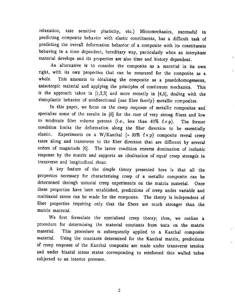
ABSTRACT

An anisotropic creep model is formulated for metallic composites withstrong fibers and low to moderate fiber volume percent (< 40%). The ideal-ization admits no creep in the local fiber direction and assumes equal creep

strength in longitudinal and transverse shear. Identification of the matrixbehavior with that of the isotropic limit of the theory permits characterization

of the composite through uniaxial creep tests on the matrix material.Constant and step-wise creep tests are required as a data base. The model

provides an upper bound on the transverse creep strength of a compositehaving strong fibers embedded in a particular matrix material. Comparison ofthe measured transverse strength with the upper bound gives an assessment ofthe integrity of the composite. Application is madeto a Kanthal composite, amodel high-temperature composite system. Predictions are made of the creepresponse of fiber reinforced Kanthal tubes under interior pressure.

INTRODUCTION

Monolithic structural alloys used in high temperature environments

(T/Tm > .3 or .4) exhibit complex thermomechanical behavior that is both

time and history dependent. The wealth of research activity over the past

decade directed toward high temperature structural alloys is testimony to these

behavioral complexities and to the need for mathematical representations

(constitutive equations) of this behavior insupp0rt of component design.

When two metallic alloys are combined to form a composite that is

exposed to high temperature, one or both of the constituents may behave

inelastically in this same time dependent, hereditary way. Although inelastic

response may be suppressed under some special conditions, viz., when a single

stress component is aligned directly with strong fibers, high temperature

response under general states of stress inevitably involves inelasticity (creep,

relaxation, rate sensitive plasticity, etc.) Micromechanics, successful in

predicting composite behavior with elastic constituents, has a difficult task of

predicting the overall deformation behavior of a composite with its constituents

behaving in a time dependent, hereditary way, particularly when an interphase

material develops and its properties are also time and history dependent.

An alternative is to consider the composite as a material in its own

right, with its own properties that can be measured for the composite as a

whole. This amounts to idealizing the composite as a psuedohomogeneous,

anisotropic material and applying the principles of continuum mechanics. This

is the approach taken in [1,2,3] and more recently in [4,5], dealing with the

viscoplastic behavior of unidirectional (one fiber family) metallic composites.

In this paper, we focus on the creep response of metallic composites and

specialize some of the results in [5] for the case of very strong fibers and low

to moderate fiber volume percent (i.e., less than 40% f.v.p). The former

condition limits the deformation along the fiber direction to be essentially

elastic. Experiments on a W]Kanthal (~ 35% f.v.p) composite reveal creep

rates along and transverse to the fiber direction that are different by several

orders of magnitude [6]. The latter condition ensures domination of inelastic

response by the matrix and supports an idealization of equal creep strength in

transverse and longitudinal shear.

A key feature of the simple theory presented here is that all the

properties necessary for characterizing creep of a metallic composite can be

determined through uniaxial creep experiments on the matrix material. Once

these properties have been established, predictions of creep under variable and

multiaxial stress can be made for the composite. The theory is independent of

fiber properties requiring only that the fibers are much stronger than the

matrix material.

We first formulate the specialized creep theory; then, we outline a

procedure for determining the material constants from tests on the matrix

material. This procedure is subsequently applied to a Kanthal composite

material. Using the constants determined for the Kanthal matrix, predictions

of creep response of the Kanthal composite are made under transverse tension

and under biaxial stress states corresponding to reinforced thin walled tubes

subjected to an interior pressure.

2

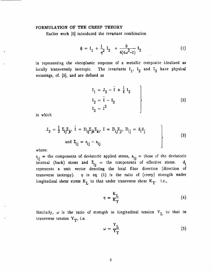
FORMULATION OF THE CREEP THEORY

Earlier work [5] introduced the invariant combination

1 9 I3¢ = I1 + _2 I2 + 4(4_-1)(1)

in representing the viscoplastic response of a metallic composite idealized as

locally transversely isotropic. The invariants I1, 12 and 13 have physical

meanings, cf. [5], and are defined as

in which

I1 = J2- _ ÷ _ I3

^

12 = I -13

13 12

(2)

1 i I= = did j ]J2 = _ _ij_ji ' = DijZjk_ki' Difiji' Dij (3)

and _]ij = sij - aij

where:

sij = the components of deviatoric applied stress, aij = those of the deviatoric

internal (back) stress and Zij = the components of effective stress, d i

represents a unit vector denoting the local fiber direction (direction of

transverse isotropy). _? in eq. (1) is the ratio of (creep) strength under

longitudinal shear stress K L to that under transverse shear K T. i.e.,

K L

,7= _T (4)

Similarly, w is the ratio of strength in longitudinal tension YL to that in

transverse tension YT' i.e.

YL

= _ (5)

As we wish to consider the case of very strong fibers, we take

w _ ® (6)

Also, reflecting low to moderate fiber volume percent, we take K L = K T = Kso that

= 1 (7)

With eqs. (6) and (7) the invariant _ becomes

3 12dp = J2- :t (8)

Guided by [5] we propose a creep representation based on the invariant ¢

and an analogous one defined as

where

(9)

1

fl_ = _ aijaji , ]= Dijaji (10)

A full statement of the proposed (isothermal) theory is as follows

4 4

F = _ dp G = _ ¢ (11)% %

(flow law) (12)eiJ = 2f(F) Fij

_o %_

aij = h(G)_o

1_° °

-r(G)

ao_/_

(evolutionary law) (13)

rij _ij- _ I(3Dij- gij)

IIij = aij- ½ J(3Dij- 6ij )

(14)

(15)

4

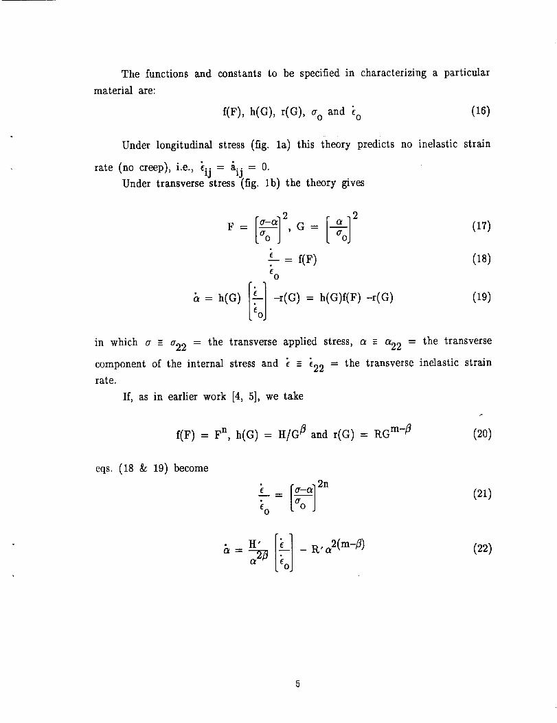
The functions and constants to be specified in characterizing a particular

material are:

f(F), h(G), r(G), a o and _o (16)

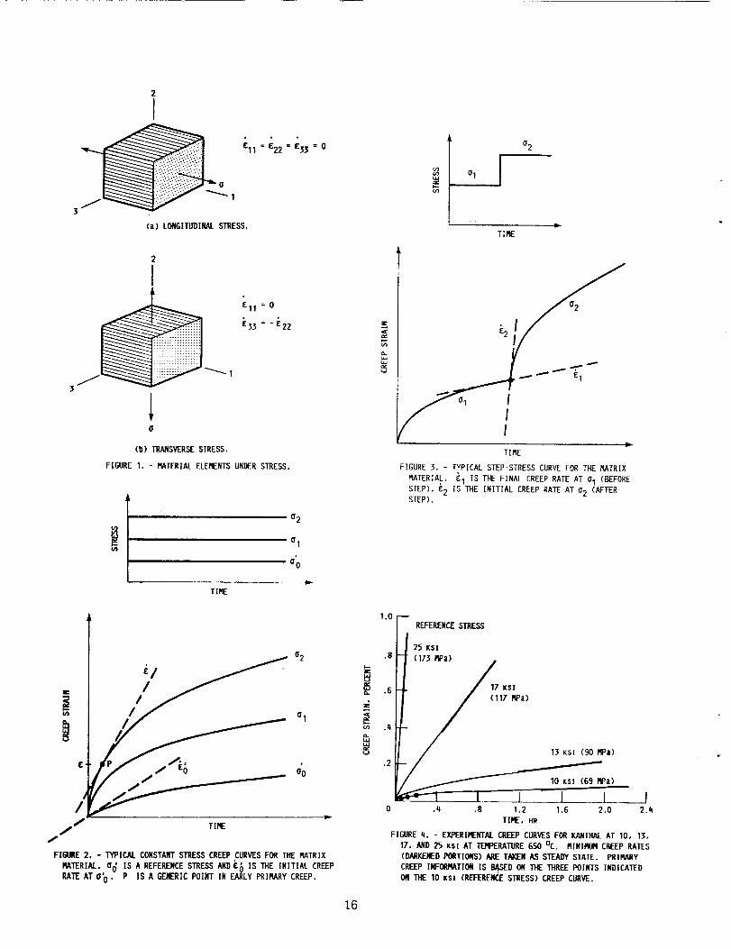
Under longitudinal stress (fig. la) this theory predicts no inelastic strain

rate (no creep), i.e., eij = £ij = 0.

Under transverse stress (fig. lb) the theory gives

2 2

L = f(F) (18)

&= h(G) [:e--o]-r(G) = h(G)f(F)-r(G)(19)

in which a = a22 = the transverse applied stress, a - a22 = the transverse

component of the internal stress and } - }22 = the transverse inelastic strain

rate.

If, as in earlier work [4, 5], we take

f(F) = Fn, h(G) = H/G fl and r(G) = RG m-fl (20)

eqs. (18 & 19) become

(21)

H' [_ol _R, a2(m-fl )(22)

5

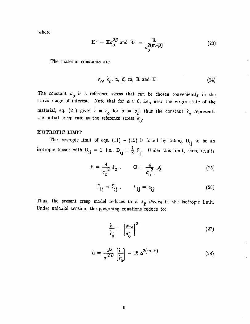
where

H' --- Ha2o _ and R' = R%2(m-Z)

(23)

The material constants are

ao' Co' n, fl, m, R and H (24)

The constant a o is a reference stress that can be chosen conveniently in the

stress range of interest. Note that for o_ _ 0, i.e., near the virgin state of the

material, eq. (21) gives _ = eo for a = ao; thus the constant eo represents

the initial creep rate at the reference stress a o.

ISOTROPIC LIMIT

The isotropic limit of eqs. (11) - (15) is found by taking Dij to be an1

isotropic tensor with Dii = 1, i.e., Dij = _ _ij" Under this limit, there results

4 4F = _ J2 ' G = _ _ (25)

g O O"O

Fij = _ij' 1-Iij = aij (26)

Thus, the present creep model reduces to a J2 theory in the isotropic limit.

Under uniaxial tension, the governing equations reduce to:

" t%J_0

(2T)

(2s)

6

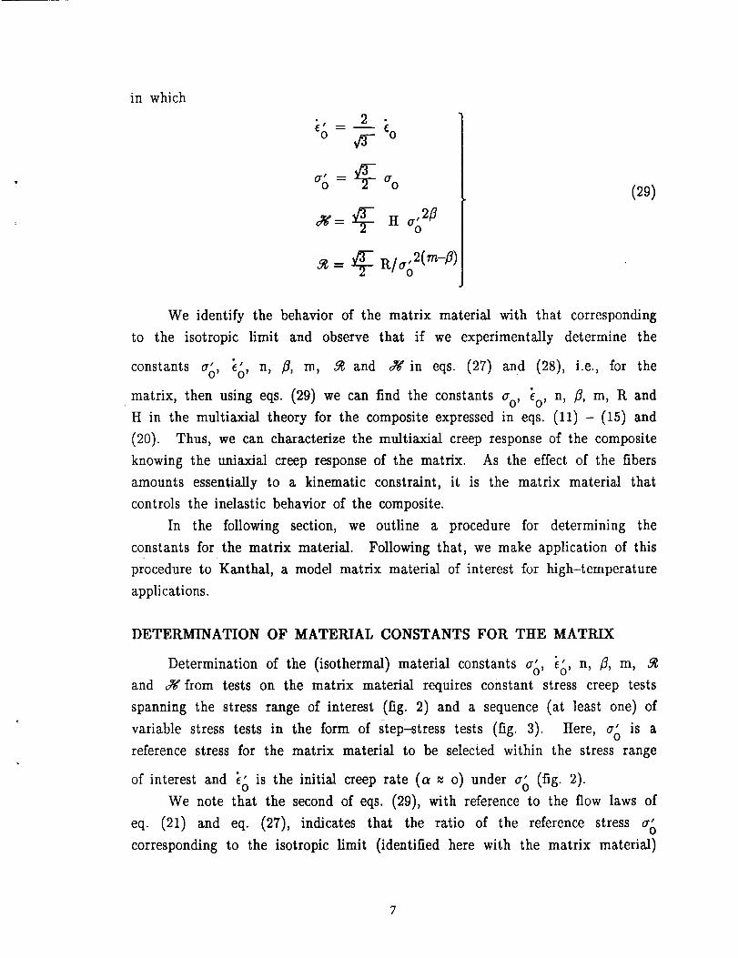
in which

Oro --_ :_ O"0

or= @ H %2Z

= @ a/Oo2(m-z)

(29)

We identify the behavior of the matrix material with that corresponding

to the isotropic limit and observe that if we experimentally determine the

constants ao, "'• Co, n, /3, m, 5_ and gg in eqs. (27) and (28), i.e., for the

matrix, then using eqs. (29) we can find the constants ao, _o' n, /3, m, R and

H in the multiaxial theory for the composite expressed in eqs. (11) - (15) and

(20). Thus, we can characterize the multiaxial creep response of the composite

knowing the uniaxial creep response of the matrix. As the effect of the fibers

amounts essentially to a kinematic constraint, it is the matrix material that

controls the inelastic behavior of the composite.

In the following section, we outline a procedure for determining the

constants for the matrix material. Following that, we make application of this

procedure to Kanthal, a model matrix material of interest for high-temperature

applications.

DETERMINATION OF MATERIAL CONSTANTS FOR THE MATRIX

Determination of the (isothermal) material constants ao, "•• Co, n, /3, m, 5_

and _ from tests on the matrix material requires constant stress creep tests

spanning the stress range of interest (fig. 2) and a sequence (at least one) of

variable stress tests in the form of step-stress tests (fig. 3). Here, a o is a

reference stress for the matrix material to be selected within the stress range

of interest and eo', is the initial creep rate (a _ o) under a o' (fig. 2).

We note that the second of eqs. (29), with reference to the flow laws of

eq. (21) and eq. (27), indicates that the ratio of the reference stress a_

corresponding to the isotropic limit (identified here with the matrix material)

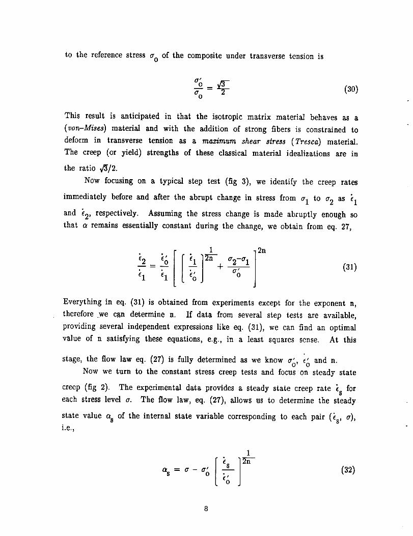
to the reference stress ¢ro of the composite under transverse tension is

°o (3o)

This result is anticipated in that the isotropic matrix material behaves as a

(von-Mises) material and with the addition of strong fibers is constrained to

deform in transverse tension as a maximum shear stress (Tresca) material.

The creep (or yield) strengths of these classical material idealizations are in

the ratio v_/2.

Now focusing on a typical step test (fig 3), we identify the creep rates

immediately before and after the abrupt change in stress from a 1 to a 2 as i 1

and i2, respectively. Assuming the stress change is made abruptly enough so

that a remains essentially constant during the change, we obtain from eq. 27,

• j

_2 eo

i I i 1

i 1b

_0

1

a2-al+_

%

2n

(31)

Everything in eq. (31) is obtained from experiments except for the exponent n,

therefore we can determine n. If data from several step tests are available,

providing several independent expressions like eq. (31), we can find an optimal

value of n satisfying these equations, e.g., in a least squares sense. At this

stage, the flow law eq. (27) is fully determined as we know ao, eo and n.

Now we turn to the constant stress creep tests and focus on steady state

creep (fig 2). The experimental data provides a steady state creep rate i s for

each stress level a. The flow law, eq. (27), allows us to determine the steady

state value a s of the internal state variable corresponding to each pair (is, a),

i.e.,

i s ] n_n--% = % .--;-eo

(32)

8

At steady state _ = 0 and the evolutionary law eq. (28) gives

es _ 2m

eo

(33)

The only unknowns in eqs. (32) and (33) are m and the ratio _/Jg. As

before, optimal values of these can be found satisfying several pairs of

equations like (32) and (33) resulting from the available test data. We now

know ao, Co' n, m and the ratio _] Jg

Now we focus on the primary creep stage. During early primary creep

the first term in eq. (28) dominates and we can write

a = a--2"-_ eo(34)

Upon integration of eq. (34) with the initial values e = 0 and a = 0 we

obtain:

o 2Z+ t (35)e=_

Again, from the flow law, eq. (27)

1

.-7_O

Now we consider a typical data point P during early primary creep as in fig.

2. At P we know the creep strain e, the creep strain rate _ , and the stress

a. Thus for a given P the only unknowns in eqs. (35) and (36) are _ and

d_'. Again, consideration of a number of data points P during early primary

creep yields optimal values of the constants _ and _.

This completesthe procedure for specifying the material constants ao, Co'

n, 8, m, _ and _ for the matrix material. As indicated earlier, use of eq.

(29) then allows determination of the constants for the composite material, eq.

(24). In the next section we present the results of applying this procedure to

Kanthal, the matrix material of a Kanthal composite.

DETERMINATION OF THE MATERIAL CONSTANTS FOR KANTHAL

The Kanthal matrix material considered here is of the following

composition by weight percentage: 73.2% Fe, 21% Cr, 5.8% A1 and 0.04% C.

The data base for Kanthal is comprised of a set of constant stress creep tests

(fig. 4) and a variable stress test (fig. 5) involving two abrupt stress steps.

The data are isothermal at 650 C; this corresponds to T/T m _ .45 for

Kanthal. The constant stress tests are at 10,13,17 and 25 ksi (69,90,117 and

173 MPa) taken over the relatively short time period < 2.2 hr with

accumulated creep strain <1%, as seen in fig 4. The short time duration of

the creep data exemplifies the cycle duration in some aerospace applications.

The creep curves show typical primary creep and the minimum creep rate (the

darkened portions of the curves) is identified as steady state for the present

purposes.

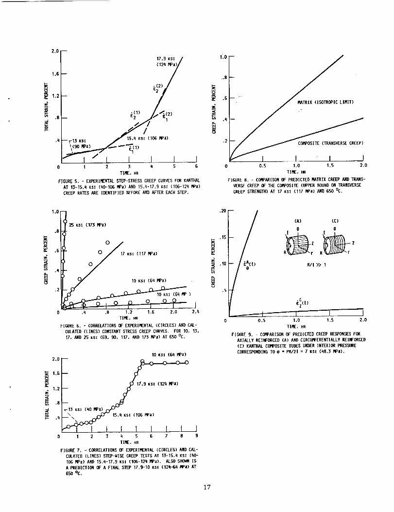
The step creep test of fig. 5 begins at 13 ksi (90 MPa) with a step to

15.4 ksi (106 MPa) at 2 hr and a second step to 17.9 ksi (124 MPa) at 4 hr;

the loading rate is 9000 ksi/hr (62100 MPa/hr). It is assumed that the stress

steps are made sufficiently abruptly so that the negligible changes occur in the

internal microstructure governing creep behavior (measured phenomenologically

by a in eqs. (27) and (28)).

The test data was processed as outlined in the foregoing section. The

"' the measuredreference stress a o was chosen as 10 ksi (69 MPa) with eo

initial creep rate at 10 ksi. Inelastic strain rates were estimated before and

after each of the two stress steps of fig. 5 giving two equations, eq. (31), from

which an optimal value of the exponent n was obtained. This was

accomplished using a Levenberg/Marquardt least squares method.

Steady state (minimum creep rate) data (is,a) were obtained from the

constant stress creep curves of fig. 4 and used in eqs. (32) and (33). Using

the same least squares method indicated above the optimal values of m and

2/,_ were obtained.

lO

Primary creep information was based on the three data points on the 10

ksi (reference stress) creep curve indicated in fig. 4. Respective measurements

of e, _ and a at these points were used in eqs. (35) and (36) similarly

providing optimal values of the constants /3 and Jg This completes the

specification of the material constants for the Kanthal matrix.

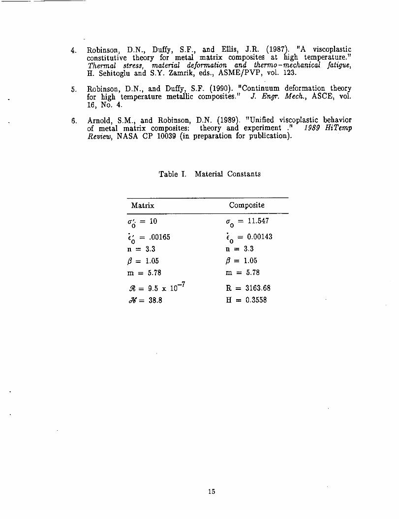
Values of the material constants for Kanthal and for a composite at

650 °C are given in Table I (the material constants values are consistent with

the units ksi and hr).

Figs. 6 and 7 show correlations of the data of figs. 4 and 5 with

calculations using the matrix constants of Table I in eqs. (27) - (29). Equiv-

alently, the calculations could be made using the composite constants of Table

I in the multiaxial forms eq. (11) - (15), (20) under the isotropic limit Dij -_1

PREDICTIONS OF THE CREEP THEORY

The predictions of this section are made using the composite constants of

Table I in eqs. (11) - (15), (20). Fig. 8 compares the Creep response of the

Kanthal matrix (isotropic limit) at 17 ksi (117 MPa) and 650 C with that

predicted for transverse creep of the Kanthal composite, i.e., after the inclusion

of strong unidirectional fibers (for example W-fibers) that suppress creep along

their direction. As indicated earlier this amounts to a kinematic constraint

that forces the matrix material, which would deform inelasticaUy as a J2

(von-Mises) material without fibers, to deform as a maximum shear stress -

Tresca material. This is reflected in the ratio of reference stresses stated in

eq. (30). Note, from eqs. (21),(27) and (29) the ratio of initial creep rates in

fig. 8 is

trans _ ]2n-1_matrix [_(37)

Here, with n = 3.3 this ratio is approximately 0.45.

The lower curve (transverse creep) in fig. 8 can be interpreted as the

creep response of the constrained matrix with no weakening from the

introduction of fiber[matrix interfacial imperfections or from the evolution of a

11

weak interphase material through diffusion. In this sense, the lower curve of

fig. 8 represents an upper bound on the transverse creep strength of the

composite. Just as a comparison of creep of the unreinforced matrix with that

of the composite along the fiber direction provides a measure of the

effectiveness of fiber strengthening, a comparison of matrix creep with that

transverse to the fibers (fig. 8) provides a measure of the integrity of the

composite. Departure from the prediction of fig. 8 may indicate possible

interracial imperfection or degradation of properties resulting from the

introduction of the fibers.

A generic point in a structure composed of a unidirectional (or

multidirectional) composite generally experiences stress components in addition

to that aligned directly with the fibers; in fact, these adverse stress

components (shear, transverse tension, etc.) control the inelastic response

(creep) of the structure. This is illustrated by the final predictions shown in

fig. 9.

Fig. 9 shows the predicted responses of (closed end) thin walled Kanthal

composite tubes subjected to an interior pressure. In one case the tube is

axially reinforced (insert A in fig 9) and the other is circumferentially re-

inforced (insert C). Each is subjected to an interior pressure p such that a =

_tR with _->>1. The axial stress is _ = a, the circumferential stress is a 0

= 2cr and the radial stress is a r _ 0.

For the axially reinforced tube (A), the governing eqs. (11) - (15), (20)

become

.A

A A ,'-'ez = r = -e0 ; "o

(38)

Integration of these equations using the composite constants Table I gives the

creep curve labelled e_(t) in fig. 9.

12

The correspondingequations for the circumferentially reinforced tube (C)

are

}C 2n•C .C __C. z _ [ a-a]

e# = 0; er = z' }o []a°

.C

H e__..z

=

2- RG m-]_ ; G =

fro

(39)

These lead to the curve labelled eC(t) in fig. 9. Clearly, the creep strength of

the circumferentially reinforced Kanthal composite tube is much greater. The

ratio of initial creep rates is

(40)

differing by almost two orders of magnitude. This large difference reflects that

the transverse stress controls the creep behavior. Transverse tension in the

axially reinforced tube (A) is a 0 = 2a ; that in the circumferentially

reinforced tube (C) is a z = a. In either case the fibers perform as expected,

• A 0 for case (A) and _ = 0 for case (C).i.e., ensuring ez =

SUMMARY AND CONCLUSIONS

An anisotropic creep model is presented for metallic composites having

strong fibers and low to moderate fiber volume percent (< 40%).

Identification of the matrix behavior with that of the isotropic limit of the

theory allows characterization of the composite through creep tests on the

matrix alone. This amounts to assuming that the fibers provide a constraint

that suppresses creep in their direction and, under transverse tension, forces

the J2 (von-Mises) matrix material to deform as a maximum shear stress

(Tresca) material. The fiber-matrix interface is assumed to be perfect without

any weakening through the introduction of fiber/matrix interfacial imperfections

13

or from the diffusion related evolution of a weak interphase material. The

prediction of transverse creep under these assumptions (fig. 8) thus provides an

upper bound on the transverse creep strength of the composite. Comparison of

the measured transverse creep response of the composite with that of the

matrix as in fig. 8 provides an assessment of the integrity of the composite.

A procedure is prescribed for characterizing the composite using creep

tests on the matrix material. The required (isothermal) data base includes

constant and step-wise constant creep tests. The procedure is applied to

Kanthal composite, a model high-temperature composite material. Creep tests

on Kanthal at 650 °C in the stress range 10-25 ksi (69-173 MPa) comprise

the data base from which the material constants are derived.

As an application of the theory, predictions are made of the creep

response of thin-walled Kanthal composite tubes (closed ends) subjected to an

interior pressure. Longitudinally and circumferentially reinforced tubes are

considered. The predictions substantiate that circumferential reinforcement is

far more efficient in limiting creep. The applications illustrate that creep is

controlled, not by the stress along the fiber direction, but by the transverse

component. This stress component is larger by a factor of two in the

longitudinally reinforced tube.

When weakening mechanisms arising from imperfect bonding, diffusion or

the fiber volume percent becomes significant and the effect of the fibers is not

limited just to a kinematic constraint as described earlier, the composite can-

not be characterized accurately on matrix testing alone. The composite should

then be modeled and tested as a material in its own right as in [4,5]. Then

the intrinsic weakening effects and their time and history dependent evolution

are appropriately reflected in the experimental results.

REFERENCES

.

.

.

Lance, R.H., and Robinson, D.N. (1971)."A maximum shear stress theoryof plasticity of fiber reinforced materials." J. Mech. Phys. Solids, 19.

Spencer, A.J.M. (1972). Deformations of fibre-reinforced materials.Clarendon Press, Oxford, England.

Spencer, A.J.M (1984). "Constitutive theory for strongly anisotropicsolids." Continuum theory of fibre-reinforced composites, Springer-Verlag,New York, N.Y.

14

.

.

.

Robinson, D.N., Duffy, S.F., and Ellis, J.R. (1987). "A viscoplasticconstitutive theory for metal matrix composites at high temperature."Thermal stress, material deformation and thermo-mechanicaI fatigue,H. Sehitoglu and S.Y. Zamrik, eds., ASME/PVP, vol. 123.

Robinson, D.N., and Duffy, S.F. (1990). "Continuum deformation theoryfor high temperature metallic composites." J. Engr. Mech., ASCE, vol.16, No. 4.

Arnold, S.M., and Robinson, D.N. (1989). "Unified viscoplastic behaviorof metal matrix composites: theory and experiment ." 1989 HiTempReview, NASA CP 10039 (in preparation for publication).

Table I. Material Constants

Matrix Composite

o'_ = 10

"" = .00165Eo

n=3.3

-- 1.05

m = 5.78

,_= 9.5 x 10 -7

J_'= 38.8

_o = 11.547

_o = 0.00143

n=3.3

= 1.05

m = 5.78

R = 3163.68

H = 0.3558

15

(a) LONG[TUDINALSTRESS.

Ell = E22 = E33 = 0 o 2

o 1

TIME

0

(b) TRANSVERSESTRESS.

F[GURE 1. - MATERIAL ELEMENTSUNDERSTRESS.

O2

O1

Oo

TIME

_'2

TIME

FIGURE 3. - TYPICAL STEP-STRESS CURVE FOR THE MATRIX

MATERIAL. El IS THE FINAL CREEP RATE AT (BEFORE

STEP), _2 IS THE INITIAL CREEP RATE AT 02 (AFTERSTEP).

f

FIGURE 2, - TYPICAL CONSTANTSTRESS CREEP CURVESFOR THE MATRIX

MATERIAL. O_ IS A REFERENCESTRESS ANB_h IS THE ]N]TIAL CREEP

RATE AT O_ . P IS A GENERIC POINT IN EARLY PRIMARY CREEP.

REFERENCESTRESS

J 125 KSI

02 .8 I-t" (173 MPa)

• _ _

i , 17 MPa)

/ 01

13 KSl (90 R°a)

E O,0 .2

,I"_ (69 VPa)I_, 1 1 [ J

/ o .. .8 1.2 1.6 2 o-----3._/ TIME = TIME, HR

J FIGURE q. - EXPERIMENTALCREEP CURVESFOR KANTHALAT 10, 13,

17, AND 25 KSl AT _KATURE 650 °C. MINIMIJM CREEP RATES

(DARKENEDPORTIONS) ARE TAKEN AS STEADYSTAE. PRIMARY

CREEP INFORMATION IS BASED ON THE THREE POINTS INDICATED

ON THE 10 KSl (REFERENCE STRESS) CREEP CURVE.

16

2.0

1,G

1.2a¢

.q

m

- 7

_ _1) L._(_,

1....._" 15.q KSZ (106 RPa)KS[

_(90 RPa) ;-" -""_'(1)

i'7 I / I I I 1 J1 2 3 II 5 G

TIRE, H9

FIGURE 5. - EXPERIENTAL STEP-STRESS CREEP CURVESFOR KANTHAL

AT 13-15.q KSl (q0-106 PPa) AND 15.q-17.9 KSZ (106-12q RPa)

CREEP RATESARE ]])ENTIFIED EFORE AND AFTER EACH STEP.

1', 0

,.8

m

.2

--, HIT)

;'_ I I " I J0.5 1.0 1.5 2,0

TIRE, HR

FIGURE 8. - COR_AR]SONOF PREDICTED NATR[X CREEP AND TRANS-

VERSE CREEPOF THE COK°OSITE (UPPER BOUNDON TRANSVERSE

CREEP STRENGTH) AT 17 KSl (117 PPa) AND 650 °C.

1,0 F1

.8L_ 25 KSl (173 RPa)

IY

,6 KS. (117 RPa)

.zl

¢P" 1oK.,

0 0

0 ._ ,8 1.2 1.5 2.0 2.e_

TIRE, HR

FIGURE 6. - CORRELATIONSOF EXPERIRENTAL(CIRCLES) AND CAL-

CULATED (LINES) CONSTANTSTRESS CREEPCURVES. FOR 10, 13,17, AND 25 KS[ (59, 90, 117, AND 173 PIPa) AT 550 °C.

2.0

1.6

1.2

.q

10 KSl (6e; RPa)

_-13 KSl (qO RPa) CTa.-'

___\ _ 15.,,Ks, IlO6_a)

I I I I I I I1 2 3 h 5 6 7 8 9

TIRE, HR

FIGURE 7. - CORRELATIONSOF EXPERTRENTAL(CIRCLES) AND CAL-

CULATED (LINES) SEP-W[SE CREEPTESTS AT 13-15.zl KS[ (z10-

105 RPa) AND 15.q-17.9 KS[ (106-124 RPa). ALSO S_ IS

A PRED]CTION OF A FINAL STEP 17.9-10 Ksz (12h--6_1 /_a) AT

650°c.

.15

.10

,5

.211--

(A) (C)

O 6

t Z

R/t>> 1

_(t)

----- I --_ I J0.5 1.0 1.5 2.0

TIRE, He

FIGURE 9. - CONPARISONOF PREDICTED CREEP RESPONSESFON

AXIALLY REINFORCED (A) AND C]RCUR:ERENT[ALLY REINFORCED

(C) KANTHALCOt_OSITE TUBES UNDERINTERIOR PRESSURE

CORRESPONDINGTO 0 = PR/2t = 7 KSt (q8.3 PIPa).

17

Report Documentation PageNational Aeronautics and

Space Administration

1. Report No, 2. GovernmentAccessionNo, 3. Reciplent's Catalog No.

NASA TM- 103172

5. ReportDate4, Titleand Subtitle

A Creep Model for Metallic Composites Based on Matrix Testing:

Application to Kanthai Composites

7. Author(s)

W.K. Binienda, D.N. Robinson, S.M. Arnold and P.A. Bartolotta

9. PerformingOrganization Name andAddress

National Aeronautics and Space AdministrationLewis Research Center

Cleveland, Ohio 44135-3191

12. SponsoringAgency Name andAddress

National Aeronautics and Space Administration

Washington, D.C. 20546-0001

6.PerformingOrganizationCode

8. PerformingOrganization Report No.

E-5550

10. WorkUnit No.

510-01-01

11. Contract or Grant No.

13. Type of Report andPeriod Covered

Technical Memorandum

14. SponsoringAgencyCode

15. SupplementaryNotes

W.K. Binienda and D.N. Robinson, University of Akron, Akron, Ohio 44325 (work funded by NASA Grant

NAG3-379). S.M. Arnold and P.A. Bartolotta, NASA Lewis Research Center.

16. Abstract

An anisotropic creep model is formulated for metallic composites with strong fibers and low to moderate fiber

volume percent (<40%). The idealization admits no creep in the local fiber direction and assumes equal creep

strength in longitudinal and transverse shear. Identification of the matrix behavior with that of the isotropic limit

of the theory permits characterization of the composite through uniaxial creep tests on the matrix material.

Constant and step-wise creep tests are required as a data base. The model provides an upper bound on the

transverse creep strength of a composite having strong fibers embedded in a particular matrix material.

Comparison of the measured transverse strength with the upper bound gives an assessment of the integrity of the

composite, Application is made to a Kanthal composite, a model high-temperature composite system. Predictions

are made of the creep response of fiber reinforced Kanthai tubes under interior pressure.

17. KeyWordsiSuggested by Author(s))

Metal matrix; Composites; High temperature;

Creep; Reference stress

lB. DistributionStatement

Unclassified- Unlimited

Subject Category 24

19. SecurityClassif.(of this report) 20. SecurityClassif.(of this page) 21. No. of pagesUnclassified Unclassified 1$

NASA FORM 1626 OCT 86 *For sale by the National Technical Information Service, Springfield, Virginia 22161

22. Price*

A03