A Coverage-Based Scheduling Algorithm for WSNs

A Coverage-Based Scheduling Algorithm for WSNs

Quazi Mamun

Received: 26 December 2012 / Accepted: 16 September 2013 / Published online: 28 September 2013

� Springer Science+Business Media New York 2013

Abstract Node scheduling in wireless sensor networks

(WSNs) plays a vital role in conserving energy and

lengthening the lifetime of networks, which are considered

as prime design challenges. In large-scaled WSNs, espe-

cially where sensor nodes are deployed randomly, 100 %

coverage is not possible all the times. Additionally, several

types of applications of WSNs do not require 100 % cov-

erage. Following these facts, in this paper, we propose a

coverage based node scheduling algorithm. The algorithm

shows that by sacrificing a little amount of coverage, a

huge amount of energy can be saved. This, in turns, helps

to increase the lifetime of the network. We provide math-

ematical analysis, which verifies the correctness of the

proposed algorithm. The proposed algorithm ensures bal-

anced energy consumption over the sensor networks.

Moreover, simulation results demonstrate that the proposed

algorithm almost doubles the lifetime of a wireless sensor

network by sacrificing only 5–8 % of coverage.

Keywords WSN � Node scheduling � Coverage �Deployment density � Coverage ratio

1 Introduction

Node scheduling algorithms are extensively used in wire-

less sensor networks (WSNs) to preserve energy con-

sumption [1–5]. In these techniques, some sensor nodes are

put in sleep mode, whereas the other sensor nodes are kept

in active mode for sensing and communication tasks. When

a sensor node is in sleep mode, it shuts down all functions,

except for a low power timer to wake itself up at a certain

time as defined by its node scheduling protocol [6].

Therefore, the sensor node consumes only a tiny fraction of

the energy, compared to the energy consumed when the

sensor node is in active mode all the time [7–9].

In WSNs, due to the limited resources and vulnerable

nature of individual sensor nodes, sensors are deployed

with high density (up to 20 nodes/m3) [10]. As a result, the

same area is covered by many sensor nodes. This causes

heavy redundancy because multiple sensor nodes consume

energy to sense the same area, and also to send/receive the

identical data. In addition, higher node density incurs more

contentions among neighbouring nodes [11]. As a result,

additional time slots are required to implement time divi-

sion multiple access (TDMA) techniques. The solution to

avoid this redundancy is to turn off the redundant nodes,

because turning off some nodes does not affect the overall

system functions as long as there are enough working

nodes to provide the services [12, 13]. Turned-off sensor

nodes save a significant amount of energy, and this

addresses one of the main constraints of WSNs, which is

limited energy. Therefore, if sensor nodes are scheduled to

perform alternately, more energy can be saved, and the

system lifetime is prolonged correspondingly. In addition

to redundancy, it is also worth mentioning that not all

applications of WSNs require 100 % coverage of the target

field [14–16]. Some 80–90 % or even a smaller amount of

coverage of the target field is adequate. For example,

applications, such as tracking humidity or temperature in

an area, detecting forest fire etc. do not require 100 %

coverage by the deployed sensor nodes. It has been shown

that sacrificing a little coverage substantially reduces the

total energy consumption of the networks [15] and thus

helps to lengthen the lifetime of the network.

Q. Mamun (&)

School of Computing and Mathematics, Charles Sturt

University, Wagga Wagga, NSW, Australia

e-mail: [email protected]

123

Int J Wireless Inf Networks (2014) 21:48–57

DOI 10.1007/s10776-013-0231-7

Following the principles described above various cov-

erage based node scheduling algorithms have been pro-

posed by researchers [12, 13, 17–20]. For example, in [17],

Xu et al. propose a node scheduling algorithm where a

subset of nodes is maintained in working mode to ensure

the desired sensing coverage. Working nodes continue

working until they run out of their energy or until they are

destroyed. A sleeping node wakes up occasionally to probe

its local neighbourhood, and starts working only if there is

no working node within its probing range. Geometrical

knowledge is used to derive the relationship between

probing range and redundancy. In this algorithm, the

authors assume that all nodes have the same sensing ranges

to calculate the desired redundancy by choosing their

corresponding probing range. However, if nodes have

different sensing ranges it is hard to find a relationship

between the probing range and the desired redundancy.

In [12], Tian and Georganas propose an algorithm that

provides complete coverage using the concept of sponsored

area. The authors present a basic model for a coverage-

based off-duty eligibility rule and back-off scheme. But the

algorithm results in more active nodes because of the

imprecise coverage degree calculation.

In [13], Ye et al. present a probing-based density control

algorithm, named PEAS, which depends on location

information to derive redundancy and allows redundant

nodes to fall asleep. In the PEAS, some nodes work con-

tinuously and die prematurely. This causes the uneven

distribution of nodes’ energy consumption across the net-

work, reducing the quality of the network coverage. Thus,

in PEAS, a sensing hole takes place permanently once it

occurs. Furthermore, it may cause partitioning of the net-

work or isolation of nodes.

PECAS [21] is a collaborating adaptive sleeping scheme

to improve PEAS. Unlike PEAS, PECAS informs the prob-

ing node of the next sleep time of a current working sensor

node in the reply message. It allows probing nodes to sub-

stitute for the current working node right after the working

nodes goes to sleep to reduce the permanent sensing holes.

From the abovementioned protocol descriptions, it is

apparent that the existing node scheduling protocols treat

coverage and connectivity separately. Moreover, the

scheduling algorithms should be aiming to achieve longer

lifetime for the network. One basic requirement for maxi-

mizing the lifetime of WSNs is to assure even distribution

of energy consumption [22, 23]. Therefore, the node

scheduling algorithm has to be designed to distribute

energy consumption properly. In addition, there are a few

more requirements for the node scheduling algorithm,

which are listed below:

1. Self-configuration of sensor nodes should be mandated

because it is inconvenient or impossible to manually

configure sensor nodes after they have been deployed

in hostile or remote working environments.

2. The design has to be fully distributed, because a

centralized algorithm needs global synchronization

overheads, and is not scalable to large populated

networks [24].

3. The scheduling algorithm should allow the maximum

number of nodes to be turned off for most of the time.

At the same time, it should preserve the required

sensing coverage.

4. The scheduling scheme should be able to maintain the

system reliability. As sensor nodes die at any time in

WSNs, a certain amount of redundancy is thus needed

to provide the reliability.

Following the above mentioned requirement, in this paper

we propose a coverage-based node scheduling protocol which

provides the required coverage maintaining minimal number

of sensor nodes, and at the same time ensuring connectivity of

the network. Each node in the network autonomously and

periodically decides itself on whether to turn on or turn off

itself using only local neighbours’ information. To preserve

sensing coverage, each node decides to turn itself off when it

discovers that it overlaps a certain amount of its sensing area

with its neighbours. The sensor nodes selected by the pro-

posed scheduling algorithm can take part constructing dif-

ferent logical topologies. For example, both in [25, 26]

multiple chains are constructed using all sensors deployed in

the target field. However, we propose that, this node sched-

uling algorithm can be run before these protocols start creat-

ing chains. Thus, a high number of sensor nodes can be turned

off, and this will save huge energy for the network.

2 Definitions and Problem Statement

Assume a set of sensor nodes @ ¼ fS1; S2; . . .g are ran-

domly deployed on a target field D. A scheduling algorithm

has to be designed so that it selects a set of sensor nodes, X,

where X � @. Based on this requirement, this section

describes the definitions of necessary terminology for the

proposed node scheduling algorithm.

Definition 1 (Sensing Region) The sensing region of a

sensor node Si, denoted as C(Si), is the amount of area that is

inside the sensing range of the sensor node Si. To make the

calculations simple, it is assumed that the sensing region of a

sensor node is represented by a circle, and all sensor nodes

have the same sensing ranges. These assumptions can be

made without the loss of generality, and are used in many

other research works, such as [27, 28].

Definition 2 (Neighbour) A node Sj is a neighbour of

node Si, if and only if sensing regions C(Sj) and C(Si)

Int J Wireless Inf Networks (2014) 21:48–57 49

123

intersect. Thus, the neighbour set of the node Si, denoted as

wðSiÞ, can be defined as: wðSiÞ ¼ fSj Sj 2 @; dðSi; SjÞ\2r;��

i 6¼ j:g where dðSi; SjÞ denotes the Euclidian distance

between the nodes Si and Sj, and where r is the radius of the

sensing region of the nodes Si and Sj.

Definition 3 (Rank) The rank of a sensor node Si, denoted

as <ðSiÞ, is defined by the cardinality of its neighbour set

wðSiÞ. Thus, if the sensor node Si has a higher number of

neighbours than the sensor node Sj, the sensor node Si’s

rank has a higher value than that of the sensor node Sj.

Definition 4 (Shared Sensing Region) Shared sensing

region of a sensor node Si, denoted as nðSiÞ, is defined as

the fraction of Si’s sensing region, that the sensor node Si

shares with its neighbouring sensor nodes. Thus, nðSiÞ ¼[fSi \ Sj 8Sj 2 wðSiÞ

�� g.

Definition 5 (Deployment Density) Deployment density,

d describes how evenly the sensor nodes are deployed in

the target field D. Assuming that @j jpr2 [ D (i.e., there are

sufficient numbers of sensor nodes to cover the target

field), deployment density d is defined as the ratio between

the maximum areas that can be covered by all disjoint

sensor nodes to the actual areas covered in the target field Dby the deployed sensor nodes.

Thus, deployment density,

d ¼ @j jpr2

[fCðSiÞ Si 2 @j g ð1Þ

Definition 6 (Coverage Ratio) Denoted by k, the coverage

ratio defines the portion of the sensor field which need to be

covered by the selected sensor nodes. Coverage ratio can be

calculated by the ratio between the total coverage area by the

selected sensor nodes to the coverage area by all deployed

sensor nodes. Obviously, increasing the coverage ratio

makes the coverage quality of the network better.

Definition 7 (k-Covered) If a point p is covered by at least

k number of sensor nodes, the point p is called k-covered.

That is, the point p’s coverage degree is k. Coverage degree

is used as the measure of quality of coverage service

(QoCS). Customarily, the higher the coverage degree, the

better the coverage quality of the network.

2.1 Problem Statement

In most relevant works, the problem about k-covered is

related to the question of how all points of the target region

would be covered by at least k number of sensor nodes.

However, for a certain kind of applications, k-covered is not

always essential. For example, some applications do not

require every point in the target field to be k-covered. This is

sufficient to achieve a certain coverage ratio. For example,

80–90 % coverage ratio, or even less is adequate for a

WSN to estimate air pressure, temperature, humidity or

to detect an event like forest fire. Moreover, when sensor

nodes are deployed randomly in a target field, the sensor

nodes may not even cover 100 % of the target area. Based

on this, a novel problem of QoCS of 1-covered with k %

coverage ratio is proposed. This paper defines the node

scheduling problem as follows: given the deployment

density d, the question is to find a minimal number of nodes

such that the coverage ratio is at least k % of the target

network.

3 Description of the Proposed Algorithm

This section describes the proposed node scheduling

algorithm in detail. The section consists of several sub-

sections which describe different issues, methods and cal-

culations for the proposed node scheduling algorithm.

3.1 Identifying Node Selection Criteria

In the proposed node scheduling algorithm, four specific

criteria have been considered. Based on these criteria, the

priority of each node is defined. For each sensor node,

these criteria are: number of neighbours of the node, the

node’s shared sensing region with its neighbours, residual

energy of the sensor node and repeated selection number of

the node (i.e., number of times the node was selected

earlier). The justifications for these criteria are described

below.

The first criterion that should be chosen for the sched-

uling algorithm is the number of neighbours of each node.

If a node does not have any neighbouring node at all, this

node must be selected. Otherwise, the sensor node’s

sensing region cannot be sensed by any other sensor

node(s). On the other hand, if a node is surrounded by

many other sensor nodes, that node’s coverage area can be

sensed by the node’s neighbouring nodes. Thus the node

with many neighbours can be turned off.

The second criterion should be the shared sensing region

ðnðxÞÞ of each sensor node with its neighbouring nodes. For

any two sensor nodes Si and Sj, the relation nðSiÞ[ nðSjÞmeans that the sensor node Si shares a comparatively larger

area with its neighbouring sensor node(s) than the sensor

node Sj does. Note that, the value nðxÞ does not depend on the

number of neighbours. Thus, if the sensing region of a node

overlaps a large amount of area with its neighbours, the node

can be replaced by one of its neighbouring nodes. As a result,

sensor nodes which share small areas with their neighbouring

nodes should have higher priority to be selected.

The third criterion to be considered during node selec-

tion is the residual energy of the sensor nodes. A sensor

50 Int J Wireless Inf Networks (2014) 21:48–57

123

node which has lost a considerable amount of its battery

energy should be avoided, unless there is no other way but

to select the node. Selecting such a node accelerates the

death of the sensor node, and this negatively affects the

network lifetime [22, 23].

The fourth and last criterion should be the repetition of

selection of a sensor node. If the same sensor node is

selected over and over again, the node loses its energy very

quickly, and his situation adversely affects the lifetime of

the network [22, 23]. Thus, the node scheduling algorithm

should be fair for each sensor, so that each sensor is

selected at least one time in a specific period of time.

After determining the node selection criteria, the next

step for the proposed node scheduling algorithm is to

construct specific rules that the algorithm would follow in

order to select appropriate sensor nodes. The following

sub-section uses the criteria discussed in this section to

construct the required set of rules.

3.2 Node Scheduling Rules

The proposed node scheduling algorithm would follow a

set of rules to schedule the sensor nodes. These rules are

derived using the selection criteria, and to meet the algo-

rithm requirements. These rules specify which node is to be

selected, which should not be selected, and which should

be prioritized. The node scheduling rules are as follows:

1. To make the node scheduling algorithm distributed and

independent from locations of sensor nodes, each node

should autonomously and periodically decide whether

to go to sleep mode, or to keep itself active. In making

this decision, each node would consider the following

issues: residual energy of the node, number of its

neighbouring nodes and number of times the node was

selected previously.

2. A sensor node with a higher level of energy holds a

higher chance of being selected than a sensor node

with a lower energy level. Otherwise, energy con-

sumption throughout the network would not be evenly

distributed.

3. A sensor node with a lower rank should be prioritized

to be selected, compared to those with higher ranks,

because a high-ranked sensor node has a higher

possibility to be redundant than a low-ranked sensor

node.

4. A sensor node which shares a comparatively smaller

area of its sensing region with its neighbouring sensor

nodes holds higher priority to be selected.

5. Among deployed sensor nodes, a set of sensor nodes

are selected by the scheduling algorithm to ensure

minimum l % of coverage by the selected sensor

nodes. On the other hand, as soon as desired l % of

coverage is achieved, the node scheduling algorithm

stops selecting any further sensor node.

After establishing the rules for scheduling sensor nodes,

the next task is to apply these rules for each sensor node.

The methods of applying the node scheduling rules for

each sensor network are described in the following sub-

section.

3.3 Applying Node Scheduling Rules to Select Sensor

Nodes

The main idea for scheduling sensor nodes is to use the

redundancy in sensing regions, and to offer the user to

select the coverage ratio (k) necessary for the specific

application. Depending on the value of coverage ratio kand deployed density d, the proposed node scheduling

algorithm is able to determine the minimum number of

sensor nodes required to achieve the coverage ratio k.

Different steps involved in the node scheduling algorithm

are described below.

In the proposed node scheduling algorithm, each sensor

node makes its own decision depending on the information

it collects from its neighbouring nodes. This decision is

made by each sensor node at the start of the node sched-

uling algorithm. To make this decision, each sensor node

generates a pseudorandom number, using the seed state that

includes two pieces of information, which are (1) residual

energy of the node, and (2) number of times the node was

previously selected. The sensor node then informs this

pseudorandom number to all of its neighbours using a

‘hello’ message. If the generated pseudorandom number is

less than a threshold value, the node decides to take part in

the scheduling process. The node then informs its will-

ingness to join the scheduling process by sending ‘notify’

messages to all of its neighbouring sensor nodes. On the

other hand, if the generated pseudorandom number is

greater than the threshold value, the sensor node does not

do anything.

A sensor node that is not participating in the scheduling

process, discards any ‘notify’ messages from its neigh-

bouring sensor nodes. On the other hand, sensor nodes

participating in the scheduling process collect all ‘notify’

messages from their neighbouring sensor nodes. From the

collected ‘notify’ messages, each participating sensor node

calculates two parameters, namely (1) its rank and (2) the

shared sensing ranges with its neighbours. These two

parameters would be used in the scheduling process in the

following way.

The rank of a sensor node is defined by the cardinality of

its neighbour set (see Sect. 2). For example, if a sensor

node does not have any neighbour, its rank is zero; if there

is a single neighbour, the rank of the node is one, and so on.


123

According to the node scheduling rules, a sensor node with

a lower rank enjoys higher priority to be selected than a

sensor node with higher rank, and vice versa. Thus node

selection procedure starts with the sensors with lower

ranks. The sensors with rank zero are considered first; after

that sensors with rank one are considered, and so on.

To consider whether a sensor node Si is to be selected or

not, its shared sensing region (nðSiÞ) with the currently

selected neighbouring sensor nodes is calculated. This is

because if a sensor node is not selected by the scheduling

algorithm, there is no point to counting the sensor node as a

neighbour. For clarification, consider the sensor node Si has

four neighbouring sensor nodes, Sm; Sn; So and Sp. Among

the neighbours, for example, the sensor nodes Sm and So

have already been selected. While the sensor node Si would

determine whether or not it would be selected, the sensor

node Si calculates nðSiÞ. In calculating nðSiÞ, the sensor

node Si considers only two of its selected neighbouring

nodes Sm and So. In other words, the sensor node Si does

not consider the sensor nodes Sn and Sp in calculating nðSiÞ.For the sensor node Si, after calculating nðSiÞ, this value is

compared with a threshold value nmax. In this proposed

node scheduling algorithm, this threshold value is called

‘maximum allowed shared sensing region’. The sensor

node is selected if nðSiÞ� nmax, otherwise the sensor node

Si is turned off.

The following two sub-sections describe how a sensor

node Si calculates nðSiÞ and how nmax value is estimated.

Note that, as it is assumed that the sensors are deployed

randomly in the target field, it is not feasible to provide a

fixed valued for nmax.

3.3.1 Shared Sensing Region Calculation

Assume the sensing range of a sensor node Si is r. By

definition, a node’s sensing region is a circle centred at this

node with radius r, if all nodes lie on a 2-D plane. To

simplify the calculation, consider only two neighbouring

nodes Si and Sj. The shared area by the two sensor nodes Si

and Si.

nðSi; SjÞ ¼ r2a� dr sinða=2Þ ¼ 2r2 arccosða=2Þ � dr sin

ðarccosðd=2rÞÞ where a is the angle created in the centre of

a sensing region by connecting two intersecting points of

the sensing regions.

Using this equation, the sensor node Si can easily find

out the shared sensing area if the sensor node Si has only a

single neighbour. However, in most of the cases, a sensor

node has more than one neighbour. Let a sensor node v has

m number of neighbours. wðSiÞ ¼ fS1; S2; . . .; Smg. Further

assume, nðSi; S1Þ ¼ A1; nðSi; S2Þ ¼ A2; . . .; nðSi; SmÞ ¼ Am:

Without loss of generality, it can be assumed that a higher

number of neighbours produce higher probability to

coincide the sensor node Si’s shared areas with its neigh-

bouring sensor nodes. Also assume, dðSi; S1Þ� dðSi; S2Þ�� dðSi; SmÞ (i.e., S1 is the closest neighbour of Si

whereas Sm is the furthest neighbour of Si). Thus, A1�A2

� � � � �Am.

To calculate the shared sensing region of Si with its

neighbour nodes, the contributions of each sensor node

(from the closest to the furthest) is considered. Essentially,

the closest neighbour contributes the most. Thus, consid-

ering the first neighbour S1; nðSiÞ ¼ A1:

Considering the second neighbour S2; nðSiÞ¼ A1 þ A2 � ðA1 \ A2Þ

Considering the third neighbour S3; nðSiÞ¼ A1 þ A2 þ A3 � ðA1 \ A2 þ A2 \ A3 þ A3 \ A1 þ A1

\ A2 \ A3Þ. . .and so on:

Now, finding the value of common areas of shared

regions (such as A1 \ A2 \ A3) is not trivial. As the number

of neighbours increases, the complexity of the computation

also increases exponentially. This computation may not be

suitable for resource constrained sensor nodes. For this

reason, a heuristic approach is adopted. This approach is

described below.

Consider the calculation of A1 \ A2. Two extreme cases

can be assumed, where in one extreme case, A1 and A2 are

disjoint. In this case the contribution of the second neigh-

bour to nðSiÞ is the whole shared area A2. On other extreme

case, the shared area of the second neighbour A2 is be fully

covered by the A1. In this case the contribution of the

second neighbour to nðSiÞ is zero. The heuristic followed in

this case is to take the average of the two extreme cases.

Thus, using this heuristic, A1 \ A2 ¼ A2

2. Therefore, after

considering the second neighbour S2; nðSiÞ ¼ A1 þ A2

�ðA1 \ A2Þ � A1 þ A2

2:

Now, applying the heuristics, A1 \ A3 þ A2 \ A3 � A1\A2 \ A3 ¼ A3

2þ A3

2� A3

3:

Therefore, after considering the third neighbour

S3; nðSiÞ ¼ A1 þ A2 þ A3 � ðA1 \ A2 þ A2 \ A3 þ A3 \ A1

þA1 \ A2 \ A3Þ � A1 þ A2

2þ A3

3:

Thus, it can be shown that the total shared sensing

region of Si with its neighbours,

nðSiÞ � nðSi; S1Þ þ1

2nðSi; S2Þ þ

1

3nðSi; S3Þ þ � � �

þ 1

mnðSi; SmÞ

¼Xm

j¼1

nðSi; SjÞj

ð3Þ

Equation (3) is used to calculate the total shared sensing

region of a sensor node Si in respect to its neighbouring

nodes which have already been selected. If the calculated


123

value of nðSiÞ is Bnmax, the sensor node Si is selected,

otherwise it is turned off. How to estimate the value of nmax

is shown below.

3.3.2 Estimate Maximum Shared Sensing Region (nmax)

Value

Selecting the value for nmax is crucial. If nmax value is too

small, the scheduling process would require a longer period

of time. On the other hand, choosing a very large nmax

actually diminishes the efficiency of the algorithm. Also

note that random deployment of the sensor nodes in the

target field precludes a predetermined value of nmax. The

value of nmax mainly depends on deployed density (d) of

the sensor nodes. Deployed density (d) is calculated using

the definitions discussed in Sect. 2. Figure 1 shows the

relationship among deployed density (d), maximum shared

sensing region allowed (nmax) and normalized coverage

ratio (k). For example, if the deployment density is 3.3, and

the user requires a coverage ratio k = 90 %, the algorithm

starts with the value of maximum shared sensing region

nmax = 25 %. Using this algorithm, however, the value of

nmax can be estimated as closely as possible. Using these

estimations and calculations, sensor nodes are selected.

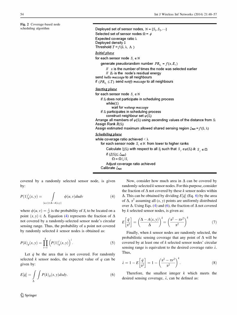
The entire node scheduling algorithm is shown in Fig. 2.

3.4 Scheduling States and Transitions

This sub-section describes the different states and their

transitions during the sensor network runs using our logical

topology. It is found in [25] that reconstruction of a chain is

required when around 20 % of its member nodes die. The

node scheduling scheme aims to engage only a subset of

the deployed nodes in the field to construct chains. Intui-

tively, this leaves an option to change the member nodes of

a chain more frequently. This helps energy dissipation by

the sensor nodes to be more evenly, and thus increases the

lifetime of the network. In the proposed node scheduling

algorithm, all the nodes stay in one of the three states: (1)

waiting state, (2) sleeping state and (3) working state.

At the very initial stage (just after the sensor deploy-

ment), or after the end of each chain construction round, all

the nodes are in waiting state. Each node waits for a ran-

dom back-off time (to avoid collisions), and then broad-

casts a ‘hello’ message. It is used for a node to collect the

pseudorandom numbers generated by its neighbour nodes.

Each node maintains a neighbour table and refreshes it

periodically. Maintaining the pseudorandom numbers of

neighbours is worthwhile when a sensor node in sleeping

state has to take part in the scheduling procedure to make

up coverage ratio.

In other words, in waiting state, a node broadcasts a ‘hello’

message. It then makes decision whether or not to take part in

the scheduling procedure, and then notifies its intension

sending a ‘notify’ message. When a node does not take part in

the scheduling procedure, it goes to sleeping mode directly

without notifying its neighbours. On the other hand, if a node

takes part in the scheduling procedure and is selected, it

enters the working state, otherwise it goes to sleeping state.

At the end of a new chain construction round, all nodes come

back to waiting state. In working state, a node actively

monitors the area and takes part in communication along the

chain. A node remains in working state until the beginning of

a chain construction round. It is assumed that when a node

fails, it simply stops working and does not send or receive

any messages.

4 Mathematical Analysis

The mathematical model is to validate the simulation

results. The results from this mathematical model will be

matched with the simulation results and compared.

Let the target field D has an area a2. Further, assume

q � D be the part of the target field D, which will be

covered by the circular sensing ranges of k number of

sensor nodes residing in the target field. Then, the ratio of

area(q) to a2, where area(q) denotes the area of q, is the

user’s desired sensing coverage at each reporting round.

Any point ðx; yÞ 2 D is considered to be covered if it is

inside the circular sensing coverage of a selected sensor

node in the target field. To measure the probabilistic

sensing coverage, the probability of a point ðx; yÞ 2 D not

to be covered by a selected sensor node Si; Pð1Þiqðx; yÞ is

measured. Let (u, v) be the location of sensor Si, and Aðx; yÞbe a circular area centred at point (x, y) with radius r. Then,

the point will not be covered when ðu; vÞ 2 D� Aðx; yÞ.Therefore, the probability of the point (x, y) not to beFig. 1 nmax versus k


123

covered by a randomly selected sensor node, is given

by:

Pð1Þiqðx; yÞ ¼Z

ðu;vÞ2D�Aðx;yÞ

/ðu; vÞdudv ð4Þ

where /ðu; vÞ ¼ 1a2 is the probability of Si to be located on a

point ðx; yÞ 2 D. Equation (4) represents the fraction of Dnot covered by a randomly-selected sensor node’s circular

sensing range. Thus, the probability of a point not covered

by randomly selected k sensor nodes is obtained as:

PðkÞqðx; yÞ ¼Yk

i¼1

Pð1Þiqðx; yÞ� �i

: ð5Þ

Let �q be the area that is not covered. For randomly

selected k sensor nodes, the expected value of q can be

given by:

E½�q� ¼Z

D

Z

PðkÞqðx; yÞdxdy: ð6Þ

Now, consider how much area in D can be covered by

randomly-selected k sensor nodes. For this purpose, consider

the fraction of D not covered by these k sensor nodes within

D. This can be obtained by dividing E½�q� (Eq. 6) by the area

of D, a2 assuming all (x, y) points are uniformly distributed

over D. Using Eqs. (4) and (6), the fraction of D not covered

by k selected sensor nodes, is given as:

E�q

a2

� �

¼ D� Aðx; yÞD

� �k

¼ a2 � pr2

a2

� �k

ð7Þ

Finally, when k sensor nodes are randomly selected, the

probabilistic sensing coverage that any point of D will be

covered by at least one of k selected sensor nodes’ circular

sensing range is equivalent to the desired coverage ratio k.

Thus,

k ¼ 1� E�q

a2

� �

¼ 1� a2 � pr2

a2

� �k

: ð8Þ

Therefore, the smallest integer k which meets the

desired sensing coverage, k, can be defined as:

Fig. 2 Coverage-based node

scheduling algorithm


123

k ¼ logð1� kÞlog a2�pr2

a2

& ’

: ð9Þ

In order to verify the correctness of k, the analytical

model is simulated, and the simulation results are

compared with the numerical results measured from

Eq. (8). Figure 3a, b show the comparison of the results

in covering a requested portion of the monitored area with

varying network sizes and sensor nodes’ circular sensing

ranges. The simulation results shown in each plot

correspond to the average of 100 simulation runs.

Regardless of the sizes of the network and sensing range,

it can be observed in Fig. 3a, b that both the numerical and

simulation results are found to match well.

5 Experimental Results

This section evaluates the performance of the proposed

node scheduling algorithm based on various experimental

results. The proposed node scheduling algorithm is com-

pared with a method which selects a same number of

sensor nodes using uniform distribution. Figure 4 shows

the comparison of the scheduling algorithm with randomly

chosen nodes from uniformly distributed nodes. For

example, to achieve the coverage ratio k = 80 % while

uniform distribution method needs around 50 nodes, the

proposed algorithm needs to select only 35 nodes to pro-

duce the same coverage ratio. Because in the proposed

algorithm, nodes are selected on the basis of shared sensing

regions, the selected nodes effectively produce better

coverage ratio.

Figure 5 shows the comparative energy consumption of

the proposed method with that of COSEN and PEGASIS.

PEGASIS is chosen in this case, because PEGASIS is also a

chain oriented algorithm which acts like COSEN, except that

it uses a single chain. To compare energy consumption, a large

value of k = 92 % is chosen. In the experiments it was found

that, by offering 92 % coverage ratio, the proposed schedul-

ing algorithm saves around 21 % energy than COSEN in 500

rounds. Figure 6 shows the network lifetime patterns using

PEGASIS, COSEN and the proposed algorithm. In PEGA-

SIS, the first node dies at around 350 rounds, and 90 % sensor

nodes die at around 600 rounds. In contrast, using COSEN, the

first nodes dies at about 400 and more than 90 % sensor nodes

die at around 550 rounds. Using the proposed algorithm

however, it was found that the first node dies at around 500

rounds and 90 % of the sensor nodes die after 875 rounds.

That means for k & 90 %, the proposed algorithm doubles

the lifetime of network. If the user requires less coverage ratio,

the lifetime can be extended even further.

In addition, to verify the effectiveness of the proposed

node scheduling algorithm, extensive simulation experi-

ments were performed to compare the performance of the

proposed algorithm with PEAS and PECAS. The reason why

these two protocols were chosen is that these two protocols

also schedule nodes based on coverage of the target field. The

Fig. 3 Comparison of simulation and analytical results for covering a target filed

Fig. 4 Comparison of proposed node scheduling algorithm with a

method which chooses nodes randomly (|@| = 100; D = 400 m

9 400 m, r = 40 m)


123

comparison was performed in terms of number of live nodes

over time period. A live node is a node which has remaining

energy and is in one of three states (working, sleeping and

waiting). In PEAS, more sensors are in working state but a

large part of their sensing area is redundantly overlapped by

their neighbours’ sensing area. Thus the sensing coverage is

not sufficient over time due to the fact that sensors die rap-

idly. In PECAS, which is an advanced version of the PEAS in

terms of energy balance, more sensors also maintain a

working state in its early stages.

PECAS has a slightly longer lifetime than PEAS. Nev-

ertheless, its sensing coverage is similar to that of PEAS with

time. It was observed that the proposed node scheduling

algorithm performed much better than PEAS and PECAS in

terms of number of live nodes over time. Figure 7 shows the

comparison among these three protocols using k = 95 % for

200 sensor deployed in a 200 m 9 200 m target field with a

deployment density of d = 1.92.

6 Conclusion

This paper proposes a coverage-based node scheduling

algorithm. The node scheduling scheme is motivated by the

reason that some applications of WSNs do not require 100 %

coverage. Furthermore, in a target field, sensor nodes are

usually deployed densely, and this creates redundancy. By

exploiting both redundancy of sensor nodes and the require-

ment of less than 100 % of coverage, the proposed member

node selection/scheduling algorithm is developed. As the

algorithm selects nodes based on neighbouring information,

the node scheduling algorithm also ensures connectivity. The

primary criteria used to schedule sensor nodes are: number of

neighbours, amount of shared sensing of the sensors, residual

energy and repetition of selection number. Simulation results

show that the proposed node scheduling algorithm saves a

significant amount of energy, while sacrificing only a little

amount of coverage. For example, the proposed scheduling

algorithm saves more than 20 % energy as compared to the

conventional chain-oriented algorithm while reducing only

7–8 % of the coverage ratio. For various applications, such as

temperature/humidity or sea level monitoring or forest fire

detection systems, where 100 % coverage is not required, this

offers a very useful trade-off to the users. The choice is kept

open for the user to calibrate the desired coverage ratio, so that

the algorithm selects minimal number of sensor nodes to

provide the coverage, at the same time warranting the con-

nectivity of the network.

Fig. 5 Energy dissipation comparison among PEGASIS, COSEN

and proposed protocol (|@| = 100; D = 50 m 9 50 m, r = 10 m,

k = 92 %, d = 2.7)

Fig. 6 Lifetime pattern comparison among PEGASIS, COSEN and

proposed protocol (|@| = 100; D = 50 m 9 50 m, r = 10 m,

k = 92 %, d = 2.7)

Fig. 7 Comparison among proposed node scheduling algorithm,

PEAS and PECAS (|@| = 200, D = 200 m 9 200 m, r = 30 m,

k = 95 %, d = 1.92)


123

References

1. Zairi, S., Zouari, B., Niel, E., Dumitrescu, E.,(2012, March).

Nodes self-scheduling approach for maximising wireless sensor

network lifetime based on remaining energy. Wireless Sensor

Systems, IET, vol.2, no.1, 52–62.

2. Liu, C., K. Wu, Y. Xiao, and B. Sun (2006, June). Random

coverage with guaranteed connectivity: joint scheduling for

wireless sensor networks. IEEE Transactions on Parallel and

Distributed Systems 17(6), 562–575.

3. Wu, K., Y. Gao, F. Li, and Y. Xiao (2005, December). Light-

weight deployment-aware scheduling for wireless sensor net-

works. Mobile Networks and Application 10(6), 837–852.

4. Buddha Singh, D. K. Lobiyal (2013). Traffic-Aware Density-

Based Sleep Scheduling and Energy Modeling for Two Dimen-

sional Gaussian Distributed Wireless Sensor Network. Wireless

Personal Communications, 70(4), 1373–1396

5. Xiao, Y., H. Li, Y. Pan, K. Wu, and J. Li (2004, November). On

optimizing energy consumption for mobile handsets. IEEE

Transactions on Vehicular Technology 53(6), 1927–1941.

6. Wang, L. and Y. Xiao (2006). A survey of energy-efficient

scheduling mechanisms in sensor networks. Mobile Networks

and Application 11(5), 723–740.

7. Bachir, A., D. Barthel, M. Heusse, and A. Duda (2006, January).

A synthetic function for energy-delay mapping in energy efficient

routing. In Third Annual Conference on Wireless On-demand

Network Systems and Services, (WONS 2006), pp. 170–178.

8. Feeney, L. and M. Nilsson (2001). Investigating the energy

consumption of a wireless network interface in an ad hoc net-

working environment. In 20th Annual Joint Conference of the

IEEE Computer and Communications Societies, (INFOCOM

2001), Volume 3, pp. 1548–1557.

9. Boaventura, Alı́rioSoares and Carvalho, NunoBorges (2013).

A Low-Power Wakeup Radio for Application in WSN-Based

Indoor Location Systems. International Journal of Wireless

Information Networks 20(1), 67–73

10. Shih, E., S. Cho, N. Ickes, R. Min, A. Sinha, A. Wang, and A.

Chandrakasan (2001, July). Physical layer driven protocol and

algorithm design for energy-efficient wireless sensor networks. In

7th ACM Annual International Conference on Mobile Computing

and Networking, (MobiCom 2001), pp. 272–287.

11. Kuo, J. C.,W. Liao, and T. C. Hou (2009, October). Impact of

node density on throughput and delay scaling in multi-hop

wireless networks. IEEE Transactions on Wireless Communica-

tions 8(10), 5103–5111.

12. Tian, D. and N. D. Georganas (2002). A coverage-preserving

node scheduling scheme for large wireless sensor networks. In

The 1st ACM International Workshop on Wireless Sensor Net-

works and Applications, pp. 32–41.

13. Ye, F., G. Zhong, S. Lu, and L. Zhang (2003, May). PEAS: A

robust energy conserving algorithm for long-lived sensor net-

works. In IEEE 23rd International Conference on Distributed

Computing Systems, (ICDCS 2003), pp. 28–37.

14. Shazly, M., Elmallah, E.S., Harms, J., AboElFotoh, H.M.F.,

(2011, October). On area coverage reliability of wireless sensor

networks, IEEE 36th Conference on Local Computer Networks

(LCN), 580–588.

15. Wang, L. and S. Kulkarni (2006). Sacrificing a little coverage can

substantially increase network lifetime. In Third Annual IEEE

Communications Society Conference on Sensor, Mesh and Ad

Hoc Communications and Networks, (IEEE SECON 2006),

pp. 326–335.

16. Megerian, B., F. Koushanfar, M. Potkonjak, and M. Srivastava

(2005, February). Worst and best-case coverage in sensor net-

works. IEEE Transactions on Mobile Computing 4(1), 84–9.

17. Xu, X., S. Sahni, and N. Rao (2008, July). Minimum-cost sensor

coverage of planar regions. In 11th International Conference on

Information Fusion, pp. 1–8.

18. Zhang, H. and J. Hou (2005). Maintaining sensing coverage and

connectivity in large sensor networks. An International Journal

on Wireless Ad Hoc and Sensor Networks 1(2), 89–124.

19. Mamun, Q., S. Ramakrishnan, and B. Srinivasan (2010 l).

Selecting member nodes in a chain oriented WSN. In IEEE

Wireless Communications and Networking Conference, (WCNC

2010), pp. 1 –6.

20. Mostafaei, Habib and Meybodi, MohammadReza (2013). A Low-

Power Wakeup Radio for Application in WSN-Based Indoor

Location Systems, International Journal of Wireless Information

Networks 20(1), 67–73.

21. Gui, C. and P. Mohapatra (2004). Power conservation and quality

of surveillance in target tracking sensor networks. In ACM Mo-

bicom 2004, pp. 129–143.

22. Shu, H., Q. Liang, and J. Gao (2008, April). Wireless sensor

network lifetime analysis using interval type-2 fuzzy logic sys-

tems. IEEE Transactions on Fuzzy Systems 16(2), 416–427.

23. Cheng, Z., M. Perillo, and W. Heinzelman (2008, April). General

network lifetime and cost models for evaluating sensor network

deployment strategies. IEEE Transactions on Mobile Computing

7(4), 484–497.

24. Zhao, S. and D. Raychaudhuri (2009, October). Scalability and

performance evaluation of hierarchical hybrid wireless networks.

IEEE/ACM Transactions on Networking 17(5), 1536–1549.

25. Tabassum, N., Q. Mamun, and Y. Urano (2006). COSEN: A

chain oriented sensor network for efficient data collection. In

Third International Conference on Information Technology: New

Generations, (ITNG 2006), pp. 262–267.

26. Mamun, Q (2013). Design Issues in Constructing Chain Oriented

Logical Topology for Wireless Sensor Networks and a Solution.

Journal of Sensors and Actuator Networks. 2, 354–387.

27. Wang, D., B. Xie, and D. Agrawal (2008, December). Coverage

and lifetime optimization of wireless sensor networks with

gaussian distribution. IEEE Transactions on Mobile Computing

7(12), 1444–1458.

28. Xiao, Y., H. Chen, K. Wu, B. Sun, Y. Zhang, X. Sun, and C. Liu

(2010, April). Coverage and detection of a randomized schedul-

ing algorithm in wireless sensor networks. IEEE Transactions on

Computers 59(4), 507–521.

Author Biography

Quazi Mamun is a Lecturer in

the School of Computing and

Mathematics, Charles Sturt

University. He earned B.Sc.

Engg. degree in Computer Sci-

ence and Engineering from

Bangladesh University of Engi-

neering and Technology

(BUET), Masters degree in

Global Information and Tele-

communication Studies from

Waseda University Japan, and

Ph.D. degree from Monash

University, Australia. Quazi’s

research interests include, but

not limited to, distributed systems, ad hoc and sensor networks,

wireless networks, and network security. He is an active member of

Advanced Networks Research Lab (ANRL) and ICT Security Group

of Charles Sturt University.


123

A Coverage-Based Scheduling Algorithm for WSNs

Documents