A coupling method for stochastic continuum models at different scales. A new approach to numerical stochastic homogenization. R. Cottereau 1 , Y. Le Guennec 1 , D. Clouteau 1 , C. Soize 2 1 Laboratoire MSSMat, ´ Ecole Centrale Paris - CNRS, France 2 Laboratoire MSME, Universit´ e Paris-Est Marne-la-Vall´ ee - CNRS, France Funding: ANR TYCHE (ANR-2010-BLAN-0904) / Digiteo - R´ egion Ile-de-France (2009-26D) R. Cottereau (ECP-CNRS) Coupling of stochastic models S´ eminaire Navier, Oct.’13 1 / 26

Welcome message from author
This document is posted to help you gain knowledge. Please leave a comment to let me know what you think about it! Share it to your friends and learn new things together.
Transcript
A coupling method for stochastic continuum models at different scales.A new approach to numerical stochastic homogenization.
R. Cottereau1, Y. Le Guennec1, D. Clouteau1, C. Soize2
1Laboratoire MSSMat, Ecole Centrale Paris - CNRS, France2Laboratoire MSME, Universite Paris-Est Marne-la-Vallee - CNRS, France
Funding: ANR TYCHE (ANR-2010-BLAN-0904) / Digiteo - Region Ile-de-France (2009-26D)
R. Cottereau (ECP-CNRS) Coupling of stochastic models Seminaire Navier, Oct.’13 1 / 26
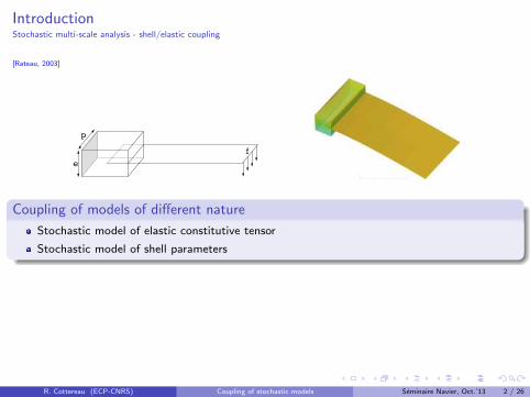
IntroductionStochastic multi-scale analysis - shell/elastic coupling
[Rateau, 2003]
f
e
p
l l l
Coupling of models of different nature
Stochastic model of elastic constitutive tensor
Stochastic model of shell parameters
R. Cottereau (ECP-CNRS) Coupling of stochastic models Seminaire Navier, Oct.’13 2 / 26
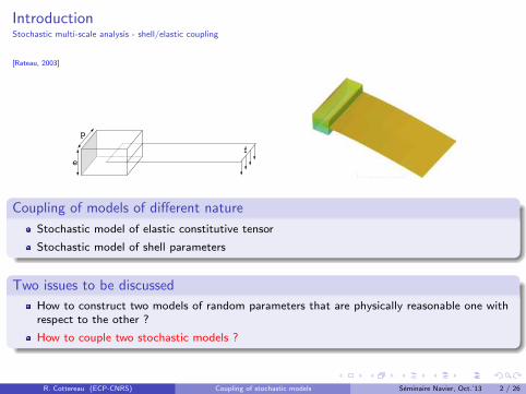
IntroductionStochastic multi-scale analysis - shell/elastic coupling
[Rateau, 2003]
f
e
p
l l l
Coupling of models of different nature
Stochastic model of elastic constitutive tensor
Stochastic model of shell parameters
Two issues to be discussed
How to construct two models of random parameters that are physically reasonable one withrespect to the other ?
How to couple two stochastic models ?
R. Cottereau (ECP-CNRS) Coupling of stochastic models Seminaire Navier, Oct.’13 2 / 26

Outline
1 Introduction
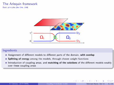
2 Coupling Stochastic models in the Arlequin frameworkDescription of the stochastic mono-modelsThe Arlequin framework
3 Stochastic-stochastic acoustic couplingDescription of the mono-modelsRandom fields of parameters at different scalesCoupling formulation: stochastic-deterministic acoustic caseCoupling formulation: stochastic-stochastic acoustic caseExample: 1D bar in traction
4 New numerical homogenization method
5 Conclusions
R. Cottereau (ECP-CNRS) Coupling of stochastic models Seminaire Navier, Oct.’13 3 / 26

Outline
1 Introduction
2 Coupling Stochastic models in the Arlequin frameworkDescription of the stochastic mono-modelsThe Arlequin framework
3 Stochastic-stochastic acoustic couplingDescription of the mono-modelsRandom fields of parameters at different scalesCoupling formulation: stochastic-deterministic acoustic caseCoupling formulation: stochastic-stochastic acoustic caseExample: 1D bar in traction
4 New numerical homogenization method
5 Conclusions
R. Cottereau (ECP-CNRS) Coupling of stochastic models Seminaire Navier, Oct.’13 4 / 26


Outline
1 Introduction
2 Coupling Stochastic models in the Arlequin frameworkDescription of the stochastic mono-modelsThe Arlequin framework
3 Stochastic-stochastic acoustic couplingDescription of the mono-modelsRandom fields of parameters at different scalesCoupling formulation: stochastic-deterministic acoustic caseCoupling formulation: stochastic-stochastic acoustic caseExample: 1D bar in traction
4 New numerical homogenization method
5 Conclusions
R. Cottereau (ECP-CNRS) Coupling of stochastic models Seminaire Navier, Oct.’13 8 / 26

Random fields of parameters at different scales
−!"# −! −$"# $ $"# ! !"#$
$"%
$"&
$"'
$"(
!
)*+,-./012345+.16!748
)*+,-./01/4*09-3:+1648
! "! #! $!−%
−#
!
#
%
&'()*)'+,-./
0.&1)*234,-−/
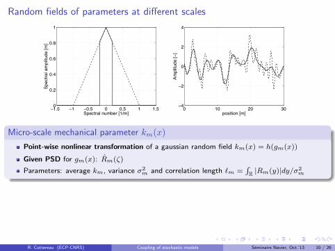
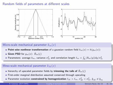
Micro-scale mechanical parameter km(x)
Point-wise nonlinear transformation of a gaussian random field km(x) = h(gm(x))
Given PSD for gm(x): Rm(ζ)
Parameters: average km, variance σ2m and correlation length ℓm =
∫
R|Rm(y)|dy/σ2
m
R. Cottereau (ECP-CNRS) Coupling of stochastic models Seminaire Navier, Oct.’13 10 / 26
Random fields of parameters at different scales
−!"# −! −$"# $ $"# ! !"#$
$"%
$"&
$"'
$"(
!
)*+,-./012345+.16!748
)*+,-./01/4*09-3:+1648
! "! #! $!−%
−#
!
#
%
&'()*)'+,-./
0.&1)*234,-−/
Micro-scale mechanical parameter km(x)
Point-wise nonlinear transformation of a gaussian random field km(x) = h(gm(x))
Given PSD for gm(x): Rm(ζ)
Parameters: average km, variance σ2m and correlation length ℓm =
∫
R|Rm(y)|dy/σ2
m
Meso-scale mechanical parameter kM (x)
hierarchy of upscaled parameter fields by trimming the tails of Rm(ζ)
First-order marginal distribution assumed conserved through upscaling
Parameter evolution constrained by homogenization ℓM > ℓm, σ2M
< σ2m, k
M6= k
m
R. Cottereau (ECP-CNRS) Coupling of stochastic models Seminaire Navier, Oct.’13 10 / 26
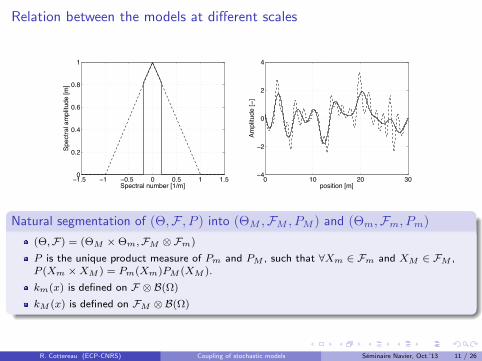
Relation between the models at different scales
−!"# −! −$"# $ $"# ! !"#$
$"%
$"&
$"'
$"(
!
)*+,-./012345+.16!748
)*+,-./01/4*09-3:+1648
! "! #! $!−%
−#
!
#
%
&'()*)'+,-./
0.&1)*234,-−/
Natural segmentation of (Θ,F , P ) into (ΘM ,FM , PM ) and (Θm,Fm, Pm)
(Θ,F) = (ΘM ×Θm,FM ⊗Fm)
P is the unique product measure of Pm and PM , such that ∀Xm ∈ Fm and XM ∈ FM ,P (Xm ×XM ) = Pm(Xm)PM (XM ).
km(x) is defined on F ⊗ B(Ω)
kM (x) is defined on FM ⊗ B(Ω)
R. Cottereau (ECP-CNRS) Coupling of stochastic models Seminaire Navier, Oct.’13 11 / 26

Examples
−!"# −! −$"# $ $"# ! !"#$
$"%
$"&
$"'
$"(
!
)*+,-./012345+.16!748
)*+,-./01/4*09-3:+1648
! "! #! $!−%
−#
!
#
%
&'()*)'+,-./
0.&1)*234,-−/
R. Cottereau (ECP-CNRS) Coupling of stochastic models Seminaire Navier, Oct.’13 12 / 26

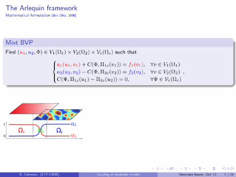
Stochastic-deterministic acoustic couplingGeneral formulation [Cottereau et al., 2011]
Mixt BVP
Find (um, uM ,Φ) ∈ Vm(Ωm)× VM (ΩM )× Vc(Ωc) such that
am(um, vm) + C(Φ, vm) = fm(vm), ∀v ∈ Vm(Ωm)
aM (uM , vM )− C(Φ, vM ) = fM (vM ), ∀v ∈ VM (ΩM )
C(Ψ, um − uM ) = 0, ∀Ψ ∈ Vc(Ωc)
,
Micro-scale stochastic acoustic model
am(u, v) = E
[∫
Ωm
αm(x)km(x, θm)∇u · ∇v dx
]
Macro-scale deterministic acoustic model
aM (u, v) =
∫
ΩM
αM (x)K∗(x)∇u · ∇v dx
Natural embedding of functional spaces
Coupling operator and mediator space to be determined
R. Cottereau (ECP-CNRS) Coupling of stochastic models Seminaire Navier, Oct.’13 13 / 26
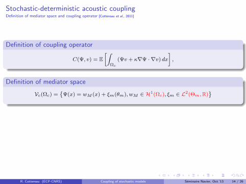
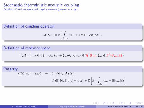
Stochastic-deterministic acoustic couplingDefinition of mediator space and coupling operator [Cottereau et al., 2011]
Definition of coupling operator
C(Ψ, v) = E
[∫
Ωc
(Ψv + κ∇Ψ · ∇v) dx]
,
Definition of mediator space
Vc(Ωc) =
Ψ(x) = wM (x) + ξm(θm), wM ∈ H1(Ωc), ξm ∈ L2(Θm,R)
R. Cottereau (ECP-CNRS) Coupling of stochastic models Seminaire Navier, Oct.’13 14 / 26
Stochastic-deterministic acoustic couplingDefinition of mediator space and coupling operator [Cottereau et al., 2011]
Definition of coupling operator
C(Ψ, v) = E
[∫
Ωc
(Ψv + κ∇Ψ · ∇v) dx]
,
Definition of mediator space
Vc(Ωc) =
Ψ(x) = wM (x) + ξm(θm), wM ∈ H1(Ωc), ξm ∈ L2(Θm,R)
Property
C(Ψ, um − uM ) = 0, ∀Ψ ∈ Vc(Ωc)
= C (E[Ψ],E[um]− uM ) + E
[
ξm
∫
Ωc
um − E[um]dx
]
R. Cottereau (ECP-CNRS) Coupling of stochastic models Seminaire Navier, Oct.’13 14 / 26
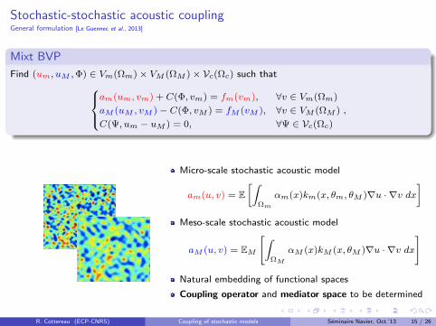
Stochastic-stochastic acoustic couplingGeneral formulation [Le Guennec et al., 2013]
Mixt BVP
Find (um, uM ,Φ) ∈ Vm(Ωm)× VM (ΩM )× Vc(Ωc) such that
am(um, vm) + C(Φ, vm) = fm(vm), ∀v ∈ Vm(Ωm)
aM (uM , vM )− C(Φ, vM ) = fM (vM ), ∀v ∈ VM (ΩM )
C(Ψ, um − uM ) = 0, ∀Ψ ∈ Vc(Ωc)
,
Micro-scale stochastic acoustic model
am(u, v) = E
[∫
Ωm
αm(x)km(x, θm, θM )∇u · ∇v dx
]
Meso-scale stochastic acoustic model
aM (u, v) = EM
[
∫
ΩM
αM (x)kM (x, θM )∇u · ∇v dx
]
Natural embedding of functional spaces
Coupling operator and mediator space to be determined
R. Cottereau (ECP-CNRS) Coupling of stochastic models Seminaire Navier, Oct.’13 15 / 26
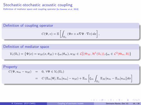
Stochastic-stochastic acoustic couplingDefinition of mediator space and coupling operator [Le Guennec et al., 2013]
Definition of coupling operator
C(Ψ, v) = E
[∫
Ωc
(Ψv + κ∇Ψ · ∇v) dx]
,
Definition of mediator space
Vc(Ωc) =
Ψ(x) = wM (x, θM ) + ξm(θm), wM ∈ L20(ΘM ,H1(Ωc)), ξm ∈ L2(Θm,R)
Property
C(Ψ, um − uM ) = 0, ∀Ψ ∈ Vc(Ωc)
= C (Em[Ψ],Em[um]− uM ) + Em
[
ξm
∫
Ωc
EM [um − Em[um]]dx
]
R. Cottereau (ECP-CNRS) Coupling of stochastic models Seminaire Navier, Oct.’13 16 / 26
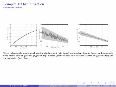
Example: 1D bar in tractionMono-models solutions
0 0.2 0.4 0.6 0.8 10
0.2
0.4
0.6
0.8
1
1.2
1.4
position x[− ]
displacemen
tum[−
]
0 0.2 0.4 0.6 0.8 10
0.5
1
1.5
2
2.5
position x[− ]
gradient∇um[−
]
0 0.2 0.4 0.6 0.8 10
0.5
1
1.5
2
2.5
position x[− ]
gra
dient∇uM[−
]
Figure: Micro-scale mono-model solution displacement (left figure) and gradient (center figure) and meso-scalemono-model solution gradient (right figure): average (dashed lines), 90%-confidence interval (grey shades) andone realization (solid lines).
R. Cottereau (ECP-CNRS) Coupling of stochastic models Seminaire Navier, Oct.’13 17 / 26

Example: 1D bar in tractionProposed approach
0 0.2 0.4 0.6 0.8 10
0.5
1
1.5
2
2.5
gradient∇w[−
]
p osition x[− ]
Figure: Gradients of the micro-scale and meso-scale solutions of the Arlequin coupled problem: average (dashedlines), 90%-confidence interval (grey shades) and one realization (solid lines).
R. Cottereau (ECP-CNRS) Coupling of stochastic models Seminaire Navier, Oct.’13 18 / 26
Outline
1 Introduction
2 Coupling Stochastic models in the Arlequin frameworkDescription of the stochastic mono-modelsThe Arlequin framework
3 Stochastic-stochastic acoustic couplingDescription of the mono-modelsRandom fields of parameters at different scalesCoupling formulation: stochastic-deterministic acoustic caseCoupling formulation: stochastic-stochastic acoustic caseExample: 1D bar in traction
4 New numerical homogenization method
5 Conclusions
R. Cottereau (ECP-CNRS) Coupling of stochastic models Seminaire Navier, Oct.’13 19 / 26
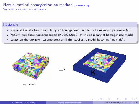
New numerical homogenization method [Cottereau, 2012]
Stochastic-Deterministic acoustic coupling
Rationale
Surround the stochastic sample by a ”homogenized” model, with unknown parameter(s);
Perform numerical homogenization (KUBC-SUBC) at the boundary of homogenized model
Iterate on the unknown parameter(s) until the stochastic model becomes ”invisible”.
⇒
c©J. Schwartz
R. Cottereau (ECP-CNRS) Coupling of stochastic models Seminaire Navier, Oct.’13 20 / 26

Proposed approach [Cottereau, 2012]
Stochastic-Deterministic acoustic coupling
Algorithm
Initialization: K0 ←− E[k]I;while ‖Ki −Ki−1‖ > criterion do
choice of modulus: K ←− Ki;resolution of Arlequin stochastic-deterministic coupled system and estimation of (u, u,Φ);update of Ki+1 so as to minimize
∫
Ω1‖∇u− I‖dx
⇒
c©J. Schwartz
R. Cottereau (ECP-CNRS) Coupling of stochastic models Seminaire Navier, Oct.’13 21 / 26
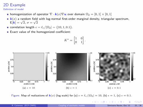
2D ExampleDefinition of model
homogenization of operator ∇ · k(x)∇u over domain Ω2 = [0, 1]× [0, 1]
k(x) a random field with log-normal first-order marginal density, triangular spectrum,E[k] =
√2, σ =
√2
correlation length ǫ = ℓc/|Ω2| = 10, 1, 0.1.Exact value of the homogenized coefficient:
K∗ =
[
1 00 1
]
.
(a) ǫ = 10 (b) ǫ = 1 (c) ǫ = 0.1
Figure: Map of realizations of k(x) (log scale) for (a) ǫ = ℓc/|Ω2| = 10, (b) ǫ = 1, (c) ǫ = 0.1.
R. Cottereau (ECP-CNRS) Coupling of stochastic models Seminaire Navier, Oct.’13 22 / 26
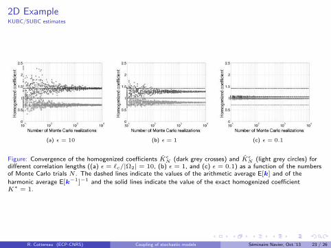
2D ExampleKUBC/SUBC estimates
(a) ǫ = 10 (b) ǫ = 1 (c) ǫ = 0.1
Figure: Convergence of the homogenized coefficients Kǫ
N(dark grey crosses) and Kǫ
N(light grey circles) for
different correlation lengths ((a) ǫ = ℓc/|Ω2| = 10, (b) ǫ = 1, and (c) ǫ = 0.1) as a function of the numbersof Monte Carlo trials N . The dashed lines indicate the values of the arithmetic average E[k] and of the
harmonic average E[k−1]−1 and the solid lines indicate the value of the exact homogenized coefficientK∗ = 1.
R. Cottereau (ECP-CNRS) Coupling of stochastic models Seminaire Navier, Oct.’13 23 / 26
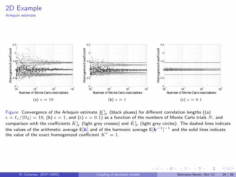
2D ExampleArlequin estimate
(a) ǫ = 10 (b) ǫ = 1 (c) ǫ = 0.1
Figure: Convergence of the Arlequin estimate Kǫ
N(black pluses) for different correlation lengths ((a)
ǫ = ℓc/|Ω2| = 10, (b) ǫ = 1, and (c) ǫ = 0.1) as a function of the numbers of Monte Carlo trials N , and
comparison with the coefficients Kǫ
N(light grey crosses) and Kǫ
N(light grey circles). The dashed lines indicate
the values of the arithmetic average E[k] and of the harmonic average E[k−1]−1 and the solid lines indicatethe value of the exact homogenized coefficient K∗ = 1.
R. Cottereau (ECP-CNRS) Coupling of stochastic models Seminaire Navier, Oct.’13 24 / 26
Conclusions
Generic coupling approach
Available for a wide range of models (potentially of different nature)
Available for deterministic-deterministic, deterministic-stochastic, stochastic-stochasticcouplings [Le Guennec et al., 2013]
(Some) mathematical analysis available [Cottereau et al., 2011]
Error estimation tools available [Zaccardi et al., 2013]
New stochastic homogenization method
Seems to work better than existing KUBC/SUBC methods for classical randomhomogenization [Cottereau, 2013]
Extendable to wider range of homogenization problems - upscaling (in particularλ-homogenization, and models of different nature)
R. Cottereau (ECP-CNRS) Coupling of stochastic models Seminaire Navier, Oct.’13 25 / 26
Bibliography
[Ben Dhia, 1998]. H. Ben Dhia (1998). Multiscale mechanical problems: the Arlequin method. Comptes Rendus de l’Acadmie des Sciences de Paris
Srie IIb 326, pp. 899-904.
[Cottereau, 2013]. R. Cottereau (2013) Numerical strategy for the unbiased homogenization of random materials. Int. J. Numer. Meth. Engr. 95,pp. 71–90
[Cottereau et al., 2011]. R. Cottereau, D. Clouteau, H. Ben Dhia, C. Zaccardi (2011) A stochastic–deterministic coupling method for continuummechanics. Comp. Meth. Appl. Mech. Engr. 200, pp. 3280–3288.
[Le Guennec et al., 2013]. Y. Le Guennec, R. Cottereau, D. Clouteau, C. Soize (2013) A coupling method for stochastic continuum models atdifferent scales. Accepted for publication in Prob. Engr. Mech.
[Rateau, 2003] G. Rateau (2003) Methode Arlequin pour les problemes mecaniques multi-echelles. PhD. Thesis, Ecole Centrale Paris, France.
[Zaccardi et al., 2013]. C. Zaccardi, L. Chamoin, R. Cottereau, H. Ben Dhia (2013) Error estimation and model adaptation forstochastic-deterministic coupling in the Arlequin framework. Accepted for publication at Int. J. Numer. Meth. Engr.
https://github.com/cottereau/CArl
R. Cottereau (ECP-CNRS) Coupling of stochastic models Seminaire Navier, Oct.’13 26 / 26
Related Documents


![Mean field for Markov Decision Processes: from …in stochastic approximation and learning [4, 1]. We also introduce an original coupling method, We also introduce an original coupling](https://static.cupdf.com/doc/110x72/5f418c5081aef224eb1404b8/mean-ield-for-markov-decision-processes-from-in-stochastic-approximation-and.jpg)