A convective weakly viscoelastic rotating flow with pressure Neumann condition

INTERNATIONAL JOURNAL FOR NUMERICAL METHODS IN FLUIDSInt. J. Numer. Meth. Fluids 2000; 00:1–6 Prepared using fldauth.cls [Version: 2002/09/18 v1.01]

A convective weakly viscoelastic rotating flow with pressureNeumann condition

Julio R. Claeyssen* ∗ Elba Bravo Asenjo** Obidio Rubio***

*IM-Promec, Universidade Federal do Rio Grande do SulP.O.Box 10673, 90001-970 Porto Alegre, RS - Brazil

**UNASP - Adventist University Center of Sao Paulo, SP - Brazil

***Facultad de Ciencias,Universidad Nacional de Trujillo, La Libertad - Peru

‡

SUMMARY

The objective of this work is to investigate through the numeric simulation the effects of the weaklyviscoelastic flow within a rotating rectangular duct subject to a buoyancy force due to the heating ofone of the walls of the duct. A direct velocity–pressure algorithm in primitive variables with a Neumanncondition for the pressure is employed. The spatial discretization is made with finite central differenceson a staggered grid. The pressure field is directly updated without any iteration. Numerical simulationswere done for several Weissemberg numbers (We) and Grashof numbers (Gr). The numerical resultsshow that for high Weissemberg numbers (We > 7.4 × 10−5) and for ducts with aspect ratio 2 : 1and 8 : 1, the secondary flow is restabilized with a stretched double vortex configuration. It is alsoobserved that when the Grashof number is increased (Gr > 17×10−4), the buoyancy force neutralizesthe effects of the Coriolis force for ducts with aspect ratio 8 : 1. Copyright c© 2000 John Wiley &Sons, Ltd.

key words: Non-newtonian; incompressible flow; mixed convection, rotating flow; finite differences

methods; pressure Neumann condition

1. Introduction

This work seeks to study the internal weakly viscoelastic flow contained in a rotatingrectangular duct with buoyancy effects due to the heating of a wall of the duct. This is donewith a direct pressure-velocity algorithm in primitive variables [1] that considers a pressureNeumann condition. This later condition is important for updating the pressure in one stepwithout any iteration. Central differences on a staggered grid are employed because they allowsecond-order approximations.

∗Correspondence to: [email protected]

Received

Copyright c© 2000 John Wiley & Sons, Ltd. Revised

2

The Navier–Stokes equations, together with the divergence free condition, constitute thebasic formulation for an incompressible flow. From a mathematical point of view, the systemthat governs this kind of flow is singular with respect to the pressure. There is no evolutionequation for such a quantity. Following the work of Gresho and Sani [2], the pressure is obtainedby solving a Poisson equation with a Neumann boundary condition. A compatibility conditionof the source with the boundary conditions guarantees the existence of solutions.

The internal rotating flow problem has been considered by several authors: Chen et al.[3], Speziale [4, 5], Robertson [6], Khayat [7], Jin and Chen [8], Nonino and Comini [9],Nonino and Croce [10], Liqiu Wao [11], Lee and Yan [12], among others. Speziale employedthe divergence-vorticity formulation with finite-difference schemes due to Arakawa for theconvective terms and the DuFort–Frankel scheme for the viscous-diffusion terms. Chen et al.,employed Fourier–Chebyshev pseudo-spectral methods for solving incompressible flows in 3Dchannels in rotation with square traversal section. Robertson, performed numerical studies forlaminar incompressible flows, in curved ducts. He employed finite differences on a staggered gridwith Newton method. Khayat studied thermal convection with viscoelastic fluids that satisfythe constitutive equations of Oldroy-B. By using the stream function–vorticity formulation,Jin and Chen [8], considered a numerical study for the transient behaviour of the naturalconvection in a vertical rectangular region. Nonino and Comini [9] and Nonino and Croce [10]treated the problem of the natural convection by using the finite element method. Liqiu [11]considered a stationary study of the transition of the bouyancy forces due to the rotation of acurved duct with a square transverse section, rotating around of a perpendicular axis to theextension of the duct. Lee and Yan [12] investigate mixed convection heat and mass transferin the entrance region of radial rotating rectangular ducts with water film evaporation alongthe porous duct walls by using a vorticity–velocity numerical method. Emphasis was placedon the rotation effects, including both Coriolis and centrifugal buoyancy forces and the massdiffusion effect on the flow structure and heat transfer characteristics.

The understanding of the pressure driven flow of a viscoelastic fluid flow is of importancein many industrial processes such as fiber spinning, injection molding, extrusion and inthe design of various types of rotating machinery. The addition of a minute amount of along chain polymer(e.g. 50-100 parts/million by weight) to a Newtonian liquid produces ahighly dilute viscoelastic liquid which can be considerably more stable in the presence ofrotations [5]. In turbulent pipe flows it results in a substantial decrease in the pressuredrop. The prediction of this behavior requires adoption of appropriate constitutive equationsand rheological parameters. Since the parameters in the constitutive equation determine theviscoelastic characteristics of flow, i.e., secondary flow patterns and volumetric flow rates,numerical prediction or measurements of velocity at certain locations can be used to estimatethese parameters [13], [14].

This work will be focused on the structure of the secondary flow and its effects on the flow inthe axial direction of the duct. It is assumed that the duct is long enough to suppress effects atthe end so that the secondary flow is independent of the coordinate along the axial direction.We shall consider two problems. The first one refers to the case of a weakly viscoelastic rotatingflow that is studied for several Weissemberg numbers [4, 5] in ducts with aspect ratio 2:1 and8:1. The other one is a mixed convection problem with a weakly viscoelastic rotating flow forseveral Grashof numbers in ducts of aspect ratio 8:1.

With the Neumann pressure condition, the results obtained by Speziale [5] for a rotatingflow have been reproduced. Specific calculations shows that the addition of of small amounts

Copyright c© 2000 John Wiley & Sons, Ltd. Int. J. Numer. Meth. Fluids 2000; 00:1–6Prepared using fldauth.cls

3

of a long chain polymer to Newtonian liquid can have a stabilizing effect on rotating channelflow and give rise to secondary flows with a substantially reduced frictional drag. This is anonlinear effect which, although observed experimentally in analogous flow configurations, toour knowledge has not been calculated in rotating channel flow. The computational experienceswith temperature effects allows observation of how the heat supplied by some mechanismgenerates flow instability with respect to earlier configurations.

2. The governing equations

In this section, we present in compact form the equations for an incompressible fluid subjectto a forcing term that will characterize the problems to be discussed in this work.

With the objective to write the equations in non-dimensional form we introduces thefollowing scales: D the length scale, W0 the velocity scale, ∆T = Th − T0 the temperaturedifference and the P0 pressure scale. We then consider the following non-dimensional variables

x1 → Dx, x2 → Dy, x3 → Dz, t∗ → DW0

t, v1 → W0u

v2 → W0v, v3 → W0w, T → T−T0

∆t, p∗ → P0P.

The non–dimensional numbers Re = W0D/ν, Pe = W0D/α are the Reynolds numberand the Peclet number, respectively. Here, ν denotes the kinematic viscosity and α is thethermal diffusion coefficient. Then the non–dimensional equations that govern the flow of anincompressible fluid are given, by the momentum equation

∂u

∂t+ u.∇u + ∇P =

1

Re∇2

u + F(u, θ), in Ω , t > 0, (1)

the continuity equation∇.u = 0, in Ω , t > 0, (2)

and the energy equation∂θ

∂t+ u.∇θ =

1

Pe

∇2θ, in Ω , t > 0 (3)

In these equations, Ω is a spatial region limited by the contour Γ, u = u(t,x) =(u(t,x), v(t,x), w(t,x)), P = P (t,x) and θ = θ(t,x) are, respectively, the velocity, thepressure, the temperature of the fluid and F is a forcing term given below for the two Maxwellviscoelastic models that are considered in this work and to be discussed in more detail insections 6 and 7.

• Model I: Rotating weakly viscoelastic flow

F(u) = (2/Ro)~j × u− 2We(∇2w∇w +

1

2∇(∇w)2), (4)

where Ro = Wo/ωD is the Rossby number and We = λν/D2 is the Weissemberg number,satisfying We << 1.

• Model II: Rotating mixed convective weakly viscoelastic flow

F(u, θ) = (2/Ro)~j × u − 2We(∇2w∇w +

1

2∇(∇w)2) +

Gr

Re2 θ~j, (5)

where Gr = gβ∆TD3/ν2 is the Grashof number, g is the gravity acceleration and β isthe coefficient of thermal expansion.

Copyright c© 2000 John Wiley & Sons, Ltd. Int. J. Numer. Meth. Fluids 2000; 00:1–6Prepared using fldauth.cls

4

Here, the rotating vector, ~ω = ωj is in the direction of the y–axis, where ω is the angularvelocity.

The problem under consideration deals with a weakly viscoelastic incompressible fluid flowcontained in a rectangular duct, driven by the pressure and subject to a permanent rotationin the direction perpendicular to the duct as considered in [4], [18]. The physical configurationand coordinate system are shown in Figure 1.

Figure 1. Flow in a rotating rectangular duct

The equations (1)–(2) are subject to the following initial and boundary conditions

u(0,x) = u0(x), x in Ω = Ω ∪ Γ, (6)

u = uΓ(x, t), on Γ = ∂Ω (7)

where u0 satisfies the continuity equation

∇.u0 = 0, in Ω (8)

and u0, uΓ being subject to the restriction

u0.n = uΓ(0,x).n, on Γ. (9)

From the continuity equation and the divergence theorem, it follows the condition of globalmass

∫

Γ

u.n dx = 0 , (10)

where n is the unit exterior normal to the boundary Γ of the region Ω.In agreement with Ladyzhenskaya [19], the specification of the pressure at the non-slip wall

of Γ is not allowed. Otherwise, the system (1)–(10) would be over determined. It is clear fromequations (1)–(2), that there is no explicit equation for the pressure. The velocity field, inprinciple, calculated from the momentum equation must be restricted so that it satisfies thesolenoidal kinematic condition ∇.u = 0. This means that the pressure has two contributions;

Copyright c© 2000 John Wiley & Sons, Ltd. Int. J. Numer. Meth. Fluids 2000; 00:1–6Prepared using fldauth.cls

5

influences it serves as a force for conservation in the mechanical balance law but, also, as acontinuity restriction [20].

For the energy equation (3), the initial condition are given

θ(x, 0) = θ0(x), x in Ω, (11)

and the mixed boundary conditions

θ = θΓ1(x, t), on Γ1 ⊂ Γ, (12)

∂θ

∂n= θΓ2

(x, t) on Γ2 ⊂ Γ, (13)

where Γ = Γ1 ∪ Γ2 is the boundary of the region Ω. Here Γ1 refers to the vertical walls of theduct and Γ2 refers to the horizontal ones.

2.1. The Poisson equation for the pressure

By applying the divergence operator in equation (2), together with the momentum equation(1), leads to the pressure equation

∇2P = ∇.

(

1

Re∇2

u − u.∇u + F(u, θ)

)

, in Ω, for t ≥ 0 (14)

Thus, the pressure is determined by solving a Poisson equation subject to appropriateboundary conditions. For the problem to be well-posed, the boundary conditions must begiven in such a way that the continuity equation is satisfied near the boundary. To keep thedivergence free condition for the velocity is an important requirement for the simulation of anincompressible flow.

The above equation is actually employed as a substitute for the continuity equation. Theelliptic nature of this equation forces the need of prescribing a boundary condition for thepressure. In a fundamental work by Gresho and Sani [2], it is concluded that a Neumanncondition for the pressure turns out to be the most appropriate. This condition is obtained bytaking the normal component of the pressure gradient isolated from the momentum equation,that is

∂P

∂n= n.∇P = n.

(

1

Re∇2

u −∂u

∂t− u.∇u + F(u, θ)

)

, on Γ, for t ≥ 0. (15)

In order that a Poisson equation (14) with a Neumann condition (15) can be solved, it isnecessary that the following compatibility condition be satisfied

∫ ∫

Ω

∇2P d Ω =

∫

Γ

Pn d Γ, (16)

where Pn = n.∇P.

3. Discretization of the Navier–Stokes Equations

When the duct is assumed to be sufficiently long, there is an internal section where the effects atthe extremes can be neglected, that is, the flow is fully developed. The axial pressure gradient

∂P

∂z= −G,

Copyright c© 2000 John Wiley & Sons, Ltd. Int. J. Numer. Meth. Fluids 2000; 00:1–6Prepared using fldauth.cls

6

is considered constant, maintained by external means (P is the modified pressure, whichincludes the gravitational and centrifugal force potentials). In this situation, it is observedthat in the internal region, the physical properties of the flow become independent of thecoordinate z, however, the fully developed velocity field is three-dimensional. For non-zerorotation rates, the components u, v of the velocity v = (u, v, w) are termed the secondary flowand the component w is referred to as the main flow.

With the above considerations, the equations (1) and (3) will be discretized with centralfinite differences on a staggered grid xi = i∆x, yj = j∆y; i = 1, . . . , N, j = 1, . . . , M on thetransverse section of the duct [21]. The spatial approximations for the pressure P , temperatureθ and the main velocity w are taken at the center of each cell. The first-order derivatives can beapproximated by forward or central differences. The notation D1r, D2r, r = x, y, is employedfor the first-order forward difference operator and for the second-order difference operator,respectively. For second-order derivatives, Dxx, Dyy correspond to the respective second–ordercentral difference operators. The pressure gradient will be approximated with a first-orderforward difference operator, while the terms with velocity by a second-order central differenceoperator. Thus, if ∇[n] and ∇2

[2] denote the discrete gradient and laplacian, respectively, we

have from the momentum equation (1) the the semi–discrete approximation

∂ui,j

∂t= −∇[1]Pi,j − ui,j .∇[2]ui,j +

1

Re∇2

[2]ui,j + F[ui,j , θi,j ]. (17)

For the energy equation (3), we have the following semi–discrete approximation

∂θi,j

∂t= − ui,j .∇[2]θi,j +

1

Pe∇2

[2]θi,j , (18)

At the boundary, the gradients and Laplacians for the velocity and energy fields areapproximated with second–order precision. This allows to have a second–order scheme throughthe closed domain Ω. Also, to improve the numerical stability when computing the pressurefrom the Poisson equation.

3.1. Time discretization

There are many available methods for time discretization. In order to reduce the computationalcost, the explicit first-order Euler method will be employed. Thus, from equation (17) we havethe time approximation scheme

uk+1i,j − u

ki,j

∆t= −∇[1]P

ki,j + U

ki,j . (19)

where

Ui,j = −ui,j .∇[2]ui,j +1

Re∇2

[2]ui,j + F[ui,j , θi,j ] (20)

In an analogous way, from equation (18), we have the time approximation scheme for theenergy equation

θk+1i,j − θk

i,j

∆t= − ui,j .∇[2]θ

ki,j +

1

Re∇2

[2]θki,j , (21)

i = 1 : N, j = 1 : M, k = 0, 1, . . .

Copyright c© 2000 John Wiley & Sons, Ltd. Int. J. Numer. Meth. Fluids 2000; 00:1–6Prepared using fldauth.cls

7

4. Discretization of the Poisson equation for the pressure

The discretization of the Poisson equation for the pressure of incompressible flows requiresspecial attention. It is required that the solution of equation (19) satisfies the continuityequation in the interior of the spatial region Ω.

Since the pressure field to be calculated is time-dependent, the discretization of the equationfor the pressure (14) is performed for an arbitrary but fixed time. This is done in conjunctionwith the Neumann condition (15) at the boundary Γ.

The pressure field is determined up to an additive constant corresponding to the levelof hydrostatic pressure. This can be removed by prescribing the integral relationship c =∫∫

ΩP (x, y)dxdy, or by a grounding condition at certain point P (x0, y0) = 0. This later

condition will be considered. Thus, for a given discrete solution Pi,j , although (Pi,j + c) isalso a solution for any constant c, the grounding condition let us to determine the pressure bychoosing c = 0.

By taking divergence in equation (19), and to keep valid the continuity equation at leveltime (k + 1), it follows that

∇2P k =∇.uk

∆t+ ∇.f(uk). (22)

where f contains all viscous and convective terms as well as the rotating term F. By applyinga second–order central difference approximation on a staggered grid, the Poisson equation (22)becomes

∇2[2]Pi,j = ∇[1].Ui,j + Dt (23)

where Ui,j is as given in (20). Here the term Dt = ∇.uk/∆t corresponds to dilatation and itis maintained with the purpose of eliminating non-linear instabilities [22, 23, 24].

On the other hand, the continuity equation (2) discretized at the level time (k + 1) must besatisfied exactly, that is

0 = D1xuk+1i−1,j + D1yvk+1

i,j−1. (24)

Dividing equation (24) by ∆t, we have the dilatation term

0 =D1xuk+1

i−1,j + D1yvk+1i,j−1

∆t= Dk+1

t . (25)

Substituting the approximated momentum equation (19) in equation (25), it follows that ateach level time k,

D1xD1xPi−1,j + D1yD1yPi,j−1 = Dt + D1xUi−1,j + D1yVi,j−1. (26)

Since the involved operators satisfy D1xD1xPi−1,j = DxxPi,j , D1yD1yPi,j−1 = DyyPi,j , itfollows from equation (26) that

∇2[2]Pi,j = D1xUi−1,j + D1yVi,j−1 + Dt, i = 1 : N, j = 1 : M. (27)

This is the discretized Poisson equation at level time k.In order to have good convergence of the approximate solution of (23), the compatibility

condition (16) should be satisfied exactly in the discrete form, that is [25, 26],

∑

i,j∈Ω

∇2Pi,j =∑

i,j∈Γ

∂Pi,j

∂n.

Copyright c© 2000 John Wiley & Sons, Ltd. Int. J. Numer. Meth. Fluids 2000; 00:1–6Prepared using fldauth.cls

8

In fact, by considering ∆x = ∆y = h in equation (27), we have

N,M∑

i,j=1

(Pi,j−1 + Pi−1,j − 4Pi,j + Pi+1,j + Pi,j+1) = h2

N,M∑

i,j=1

Dt + (28)

+ h

N,M∑

i,j=1

(Ui,j − Ui−1,j + Vi,j − Vi,j−1).

It turns out that

N∑

i=1

(Pi,0 − Pi,1 + Pi,M+1 − Pi,M ) +

M∑

j=1

(P0,j − P1,j + PN+1,j − PN,j) (29)

= h

N∑

i=1

(Vi,M − Vi,0) +

M∑

j=1

(UN,j − U0,j).

From the above equation, the discrete Neumann conditions should satisfy the four followingrelationships

P0,j = P1,j − hU0,j , j = 1, . . . , M (30)

PN+1,j = PN,j + hUN,j, j = 1, . . . , M (31)

Pi,0 = Pi,1 − hVi,0, i = 1, . . . , N (32)

Pi,M+1 = Pi,M − hVi,M , i = 1, . . . , N. (33)

Let us observe that these conditions are a discrete version of equation (15).

5. A pressure–velocity algorithm

We shall follow an algorithm introduced by Claeyssen et al.[1]. At each time level, the pressureis updated in one step and then the velocity field is calculated. The pressure is initialized bysolving a singular system that appears from the discretization of the Poisson equation with aNeumann condition. When solving the Poisson equation, a special treatment is given to theinterior points that correspond to the interior cells and to the adjacent cells, in such a waythat the compatibility condition is verified. This actualization contains correction terms fora direct computing of the pressure at the interior points of the interior cells. This is doneby incorporating the values of the pressure already calculated in neighboring points. Thisprocedure is described as follows.

Let u = ui,j , and P = Pi,j . The pressure is initialized by solving the equation

∇2[2]P = Dt + ∇[1].

(

−uk.∇[2]u

k +1

Re∇2

[2]uk

)

(34)

with a SOR method for k = 0 [1].For a direct up–date of the variables equation (17) is used.Let us assume that all discrete variable are known at the time k. We consider v

∗ as thevelocity that would appear as the solution of equation (17) with an absent pressure gradient

Copyright c© 2000 John Wiley & Sons, Ltd. Int. J. Numer. Meth. Fluids 2000; 00:1–6Prepared using fldauth.cls

9

by knowing the field uk, that is

v∗ − u

k

∆t1= −u

k.∇[2]uk +

1

Re∇2

[2]uk + F[uk, θk]. (35)

Thus

v∗ = u

k + ∆t1

(

−uk.∇[2]u

k +1

Re∇2

[2]uk + F[uk, θk]

)

. (36)

The variable v∗ is known as pseudo–velocity [9], and does not necessarily satisfies the

continuity equation. The Helmholtz theorem [27, 28] allows v∗ to be written as

v∗ = r∇P k+1 + A, such that ∇.A = 0. (37)

Now, defining the velocity at time (k + 1) as uk+1 = A, and the step of time as ∆t = r, it

follows, by using (36), the discrete version of (17), with ∆t1 = ∆t,

uk+1 − u

k

∆t= −∇[1]P

k+1 − uk.∇[2]u

k +1

Re∇2

[2]uk + F[uk, θk]. (38)

Thus, uk+1 is a discrete solution of equation (17) and satisfies the continuity equation.

Now, by taking divergence in (38), we arrive to the following discrete equation for thepressure at the level time (k + 1)

∇2[2]P

k+1 =∇.vk

∆t+ ∇[1].

(

−uk.∇[2]u

k +1

Re∇2

[2]uk + F[uk, θk]

)

(39)

= ∇.Uk + Dkt .

The fictitious values that appear in the discretization of the Neumann condition (30)–(33),are calculated through the following equations

P k+10,j = P k

1,j − hUk0,j , j = 1, . . . , M (40)

P k+1N−1,j = P k

N,j + hUkN,j, j = 1, . . . , M (41)

P k+1i,0 = P k

i,1 − hV ki,0, i = 1, . . . , N (42)

P k+1i,M+1 = P k

i,M − hV ki,M , i = 1, . . . , N. (43)

For the interior points, the pressure field is up–dated by solving equation (39) with theincorporation of values already determined, that is, we consider the one step scheme forcomputing the pressure field

P k+1i,j =

1

4

(

P k+1i,j−1 + P k+1

i−1,j + P ki+1,j + P k

i,j+1 + h2∇[1]Uk + h2Dk

t

)

(44)

where ∆x = ∆y = h.

5.1. The pressure–velocity algorithm

With the above discussion, an algorithm for integrating the Navier–Stokes equations for arotating flow with a prescribed Neumann condition for the pressure can be formulated asfollows.

Copyright c© 2000 John Wiley & Sons, Ltd. Int. J. Numer. Meth. Fluids 2000; 00:1–6Prepared using fldauth.cls

10

1. Introduction of the initial velocity, corresponding to the initial time level k = 0, theboundary conditions and involved physical parameters,

2. Initialization of the pressure through equation (34),3. Calculation of the pseudo–velocity field v∗ by using (36),4. One step up-dating of the pressure field by using (40)–(44),5. Up-date the temperature field θk+1 through (21),6. Up-date of the velocity field u

k+1 through (??),7. To do steps (3) - (6) for k = 1, 2, . . .8. End the calculations.

6. Rotating weakly viscoelastic flow

The model considered in this work appears in turbo machinery where we can suppose thata substance through spinning can be dissolved to form a solution. It is assumed that a smallamount of polymer added to a Newtonian liquid can create a highly diluted viscoelastic fluid,which can be considerably more stable in the presence of rotations. The prediction of thebehavior requires adoption of appropriate constitutive equations and rheological parameters.Constitutive equations can be formulated for viscoelastic fluids in terms of the mechanicalMaxwell models. The rheological behaviour of a viscoelastic fluid can be simulated by aHookean spring in series with a Newtonian viscous dashpot [30]. We shall refer to Joseph[31] for the derivation of the following constitutive equation

σ = −p1 + τ, (45)

λDτ

Dt+ τ = 2µD[u]. (46)

Here σ(t,x) is a symmetric tensor field, v(t, x) is a solenoidal field, τ is the so called extratensor and p is the reaction pressure. The type of invariant derivative that is chosen for D/Dtdetermines the form of constitutive equation. Thus, there are a great variety of possibilitiesfor this (see Joseph,1990 pp.10). In this work we shall use the covariant convected derivativeor sub convective derivative Dτ/Dt = τ with

τ =dτ

dt+ τL + L

T τ. (47)

where L is the velocity gradient. In terms of components

τokl =

∂τkl

∂t+ v.∇τkl + τkm

∂vm

∂xl

+ τlm

∂vm

∂xk

, (48)

For a fully developed flow with the above viscoelastic fluid and for which the physicalvariables are axially independent, the tensor components of a Maxwell viscoelastic flow aresimplified.

We assume that the the relaxation time λ of the weakly viscoelastic fluid is small and thatthe secondary flow is relatively weak, that is

λν

D2<< 1,

U

W<< 1,

V

W<< 1. (∗)

Copyright c© 2000 John Wiley & Sons, Ltd. Int. J. Numer. Meth. Fluids 2000; 00:1–6Prepared using fldauth.cls

11

where U, V W are maximum values for the components of the velocity field, D is the lengthscale.

The fact of having a highly diluted fluid, suggests that the specific mass ρ and the kinematicviscosity ν = µ/ρ will be the same ones as the Newtonian fluid, from which they are obtained.The hypothesis (*), implies after an order approximation analysis, that the components of thedissipative stress tensor can be approximate for the following equations:

τzz = 0,

and

τxx + 2λτxz

∂w

∂x= 2µ

∂u

∂x

τxy + λ

(

τxz

∂w

∂y+ τyz

∂w

∂x

)

= µ

(

∂u

∂y+

∂v

∂x

)

τxz + λτzz

∂w

∂x= µ

∂w

∂x

τyy + λτyz

∂w

∂y= 2µ

∂v

∂y

τyz + λτzz

∂w

∂y= µ

∂w

∂y

Denoting by ν = µ/ρ the kinematic viscosity, (∇w)2 = (∂w/∂x)2

+ (∂w/∂y)2

the value ofthe longitudinal velocity gradient, using the continuity equation and by substituting in thebalance momentum equation

ρ

[

∂v

∂t+ v.∇v + 2~ω × v

]

= −∇p + ∇ · τ

we have

∂u

∂t+ u

∂u

∂x+ v

∂u

∂y= −

1

ρ

∂p

∂x+ ν∇2u − 2λν

(

∂w

∂x∇2w +

1

2

∂

∂x(∇w)2

)

− 2ωw,

∂v

∂t+ u

∂v

∂x+ v

∂v

∂y= −

1

ρ

∂p

∂y+ ν∇2v − 2λν

(

∂w

∂y∇2w +

1

2

∂

∂y(∇w)2

)

,

∂w

∂t+ u

∂w

∂x+ v

∂w

∂y= −

1

ρ

∂p

∂z+ ν∇2w + 2ωu.

Based on the above assumptions and in dimensionless form, we obtain the following model

∂u

∂t+ u.∇u + ∇P =

1

Re∇2

u + F(u), in Ω , t > 0, (49)

∇.u = 0, in Ω , t > 0, (50)

u = (u(t, x, y), v(t, x, y), w(t, x, y)),

F(u) = (2/Ro)~j × u− 2We(∇2w∇w +

1

2∇(∇w)2), (51)

that will be employed for determining the secondary flow in a transversal section (0, D)×(0, H)perpendicular to the axis of the duct as in the Figure 1. The aspect ratio is given for χ = H/D.

Copyright c© 2000 John Wiley & Sons, Ltd. Int. J. Numer. Meth. Fluids 2000; 00:1–6Prepared using fldauth.cls

12

6.1. Numerical simulations

Here we consider the results of the numerical simulations for a rotating weakly viscoelasticfluid in a duct by using the direct velocity-pressure algorithm given before with a Neumanncondition for the pressure. The objective is to examine the effects of rotation on the secondaryflow in ducts with aspect ratio 8:1 and 2:1. In the first case, a uniform grid of 16× 128 pointswas considered, where ∆x = ∆y = 0.01ft. For the duct of ratio 2:1, a grid of 32 × 64 pointswas used, where ∆x = ∆y = 0.005ft. The results were accomplished by choosing a time step∆t = 0.001 in order to arrive quickly to the fully developed flow. This time step value satisfiesthe classical linear stability condition [5, 22]. Through numerical experiments, on a series ofrefined grids, we obtained that the solution converged to a grid-independent solution. Two basicfacts contributed for this. The spatial scheme, including the discretization at the boundary,turned out to be of second-order. The one-step update, besides the discrete compatibility ofthe pressure Neumann condition, introduces a filtering that is useful for obtaining a desirednumerical convergence.

We consider the initial velocity field conditions u(0) = v(0) = 0 and w(0) = w1, where w1

is determined by solving the Poisson equation

−∆w1 = Re C, (52)

subject to a non–slip boundary condition w = 0 on Γ. Thus, w1 corresponds to a classical quasi-parabolic profile. At the walls of the duct, were prescribed the conditions u = 0, v = 0, w = 0.

Speziale [5], mentions a qualitative comparison of this type of secondary flow with aNewtonian structure when the Weissenberg number is included. However, he does not exhibitgreater results about the structure of this flow for weakly viscoelastic fluids. It leaves as aproposal for future studies. In this work we shall exhibit the flow mentioned by Speziale.

In the case of aspect ratio 8:1, simulations were carried out for three physical situationsobtained by a variation of the Weissenberg number, while keeping fixed the other bulkproperties of the fluid such as specific mass ρ = 1.936slugs/ft3 and viscosity ν = 1.1 ×

10−5ft2/sec, corresponding to water at an environment mean temperature. The longitudinalpressure gradient is kept constant G = 2×10−4lb/ft3. For a weak rotation, it is considered theangular velocity ω = 0.005 rad/s. These later parameters correspond to the flow of a Newtonianfluid [4, 32]. They will be compared with the structure of a weak rotating viscoelastic fluid bycontrolling the Weissenberg number.

In the first situation, we chose We = 4.2969×10−5, that corresponds to the relaxation timeof λ = 0.1 (s). The secondary flow is shown for different times in Figure 2. It can be observedthat the secondary flow develops slower than in the case of a Newtonian flow [4, 32], until itreaches a fully developed state in approximately t = 4000s.

In Figure 3 are shown the streamlines of the velocity field for We = 1.289×10−4, (λ = 0.3).It is observed that the secondary flow tends to stabilize with only two vortexes, in the centerof the transversal section. The vortexes begin to appear in approximately t = 1600s, reachingthe stationary state in approximately t = 3000s. This structure differs from the previous case,where 6 vortexes are developed.

The longitudinal velocity profiles, fully developed, in the central lines of the transversalsection of the duct, for We = 1.289 × 10−4, are shown in Figure 4. The horizontal profile isfor y/D = 4 and vertical one for x/D = 0.5. It can be observed that the appearance of twovortexes in the center of the duct, generates a deviation of the horizontal profile in the direction

Copyright c© 2000 John Wiley & Sons, Ltd. Int. J. Numer. Meth. Fluids 2000; 00:1–6Prepared using fldauth.cls

13

of the side x/D = 1. However, the flowrate is reduced with a change rate of approximately 3.5% in relation to the flowrate of the longitudinal flow. The profiles, for We = 4.2969 × 10−5,have a very similar behavior to the Newtonian case [4, 32] and they are not shown here.

With a further increase of the viscoelastic coefficient, say We = 2.1484 × 10−4 (λ = 0.5),we are able to stabilize the secondary flow with a structure of two vortexes at the ends, ascan be observed in Figure 5. The fully developed state is reached in approximately t = 600s,a very smaller time in relation to the other preceding cases. This state is commented on bySpeziale [5], without presenting results, saying that for a larger Weissenberg number, satisfyingWe > 7.4 × 10−5, the flow structure stabilizes with two vortexes.

The longitudinal velocity profiles, at the central lines of the transversal section of the duct,are exhibited in Figure 6 for We = 2.1484 × 10−4 with a flowrate of approximately 2.7 %in the longitudinal direction. It is observed that when the Weissenberg number increases, thesecondary flows of a dilute, weakly viscoelastic fluid generate a reduction in the loss of theflowrate in the longitudinal direction, as shown in Figures 4 and 6, in comparison to thereduction of 7 %, that happens in the case of a Newtonian fluid [4, 32].

In Figures 7 and 8, are shown the velocity fields and streamlines of the secondary flow, in aduct with a aspect ratio 2 : 1, for We = 1.289×10−4, with angular velocity ω = 0.1 rad/s, anda longitudinal velocity gradient G = 6× 10−4lb/ft3. It is observed that for weakly viscoelasticfluids, besides the two main vortexes, there appear two secondary vortexes in the mediumsection of the duct (Figure 8 d). The secondary vortexes are dissipated and after a certainperiod of instability, the flow is able to stabilize in two counter-rotating vortexes.

The longitudinal velocity profiles can be seen in Figure 9, where the flowrate, due to theeffects of this secundary flow, is of 48.6 % relative to the flowrate without rotation.

2 4 6 8 10 12 14 16

20

40

60

80

100

120

0 0.1 0.2 0.3 0.4 0.5 0.6 0.7 0.8 0.9 10

1

2

3

4

5

6

7

8

0 0.1 0.2 0.3 0.4 0.5 0.6 0.7 0.8 0.9 10

1

2

3

4

5

6

7

8

0 0.1 0.2 0.3 0.4 0.5 0.6 0.7 0.8 0.9 10

1

2

3

4

5

6

7

8

0 0.1 0.2 0.3 0.4 0.5 0.6 0.7 0.8 0.9 10

1

2

3

4

5

6

7

8

(a) (b) (c) (d) (e)

Figure 2. Streamlines of the secondary flow in a duct with aspect ratio 8:1; for t: (a)10s, (b) 500s, (c) 1000s, (d) 1600s (e) fully developed, for Re = 248, C = 0.057

(G = 2 × 10−4lb/ft3), Ro = 21.3 (ω = 0.005rad/seg) We = 4.2969 × 10−5.

Copyright c© 2000 John Wiley & Sons, Ltd. Int. J. Numer. Meth. Fluids 2000; 00:1–6Prepared using fldauth.cls

14

2 4 6 8 10 12 14 16

20

40

60

80

100

120

0 0.1 0.2 0.3 0.4 0.5 0.6 0.7 0.8 0.9 10

1

2

3

4

5

6

7

8

0 0.1 0.2 0.3 0.4 0.5 0.6 0.7 0.8 0.9 10

1

2

3

4

5

6

7

8

0 0.1 0.2 0.3 0.4 0.5 0.6 0.7 0.8 0.9 10

1

2

3

4

5

6

7

8

0 0.1 0.2 0.3 0.4 0.5 0.6 0.7 0.8 0.9 10

1

2

3

4

5

6

7

8

(a) (b) (c) (d) (e)

Figure 3. Streamlines of the secondary flow in a duct with aspect ratio 8:1; for t: (a)10s, (b) 500s, (c) 1000s, (d) 1600s (e) fully developed, for Re = 248, C = 0.057

(G = 2 × 10−4lb/ft3), Ro = 21.3 (ω = 0.005rad/s), We = 1.289 × 10−4.

0 0.2 0.4 0.6 0.8 1 1.2 1.4 1.6 1.80

0.1

0.2

0.3

0.4

0.5

0.6

0.7

0.8

0.9

1

0 0.2 0.4 0.6 0.8 1 1.2 1.4 1.6 1.80

1

2

3

4

5

6

7

8

(a) (b)

Figure 4. Axial velocity profiles in a duct 8:1; Re = 248, C = 0.057, Ro = 21.3:(a) horizontal, (b) vertical, dashed lines for λ = 0 and continuous lines for λ = 0.3,

We = 1.289 × 10−4, Qf

Q= 0.9654.

Copyright c© 2000 John Wiley & Sons, Ltd. Int. J. Numer. Meth. Fluids 2000; 00:1–6Prepared using fldauth.cls

15

2 4 6 8 10 12 14 16

20

40

60

80

100

120

0 0.1 0.2 0.3 0.4 0.5 0.6 0.7 0.8 0.9 10

1

2

3

4

5

6

7

8

0 0.1 0.2 0.3 0.4 0.5 0.6 0.7 0.8 0.9 10

1

2

3

4

5

6

7

8

0 0.1 0.2 0.3 0.4 0.5 0.6 0.7 0.8 0.9 10

1

2

3

4

5

6

7

8

(a) (b) (c) (d)

Figure 5. Streamlines of the secondary flow in a duct with aspect ratio 8:1; for t: (a) 10s,(b) 500s, (c) 1600s (d) fully developed, for Re = 248, C = 0.057 (G = 2×10−4lb/ft3),

Ro = 21.3 (ω = 0.005rad/s), We = 2.1484 × 10−4.

0 0.2 0.4 0.6 0.8 1 1.2 1.4 1.6 1.80

0.1

0.2

0.3

0.4

0.5

0.6

0.7

0.8

0.9

1

0 0.2 0.4 0.6 0.8 1 1.2 1.4 1.6 1.80

1

2

3

4

5

6

7

8

(a) (b)

Figure 6. Axial velocity profiles in a duct 8:1; Re = 248, C = 0.057,Ro = 21.3: (a)horizontal, (b) vertical, with dashed lines for λ = 0 and continuous lines for λ = 0.5,

We = 2.1484 × 10−4, Qf

Q= 0.9735.

Copyright c© 2000 John Wiley & Sons, Ltd. Int. J. Numer. Meth. Fluids 2000; 00:1–6Prepared using fldauth.cls

16

0.1 0.2 0.3 0.4 0.5 0.6 0.7 0.8 0.9

0.2

0.4

0.6

0.8

1

1.2

1.4

1.6

1.8

0.1 0.2 0.3 0.4 0.5 0.6 0.7 0.8 0.9

0.2

0.4

0.6

0.8

1

1.2

1.4

1.6

1.8

0.1 0.2 0.3 0.4 0.5 0.6 0.7 0.8 0.9

0.2

0.4

0.6

0.8

1

1.2

1.4

1.6

1.8

(a) (b) (c)

0.1 0.2 0.3 0.4 0.5 0.6 0.7 0.8 0.9

0.2

0.4

0.6

0.8

1

1.2

1.4

1.6

1.8

0.1 0.2 0.3 0.4 0.5 0.6 0.7 0.8 0.9

0.2

0.4

0.6

0.8

1

1.2

1.4

1.6

1.8

0.1 0.2 0.3 0.4 0.5 0.6 0.7 0.8 0.9

0.2

0.4

0.6

0.8

1

1.2

1.4

1.6

1.8

(d) (e) (f)

Figure 7. Secondary flow in a duct 2:1; t= (a) 1s, (b) 12.5s, (c) 40s , (d) 75s, (e)400s, (f) fully developed,for Re = 279, C = 0.1345 (G = 6 × 10−4lb/ft3), Ro = 1.198 (ω = 0, 1rad/s), We = 1.289 × 10−4.

0 0.1 0.2 0.3 0.4 0.5 0.6 0.7 0.8 0.9 10

0.2

0.4

0.6

0.8

1

1.2

1.4

1.6

1.8

2

x/D

y/D

0 0.1 0.2 0.3 0.4 0.5 0.6 0.7 0.8 0.9 10

0.2

0.4

0.6

0.8

1

1.2

1.4

1.6

1.8

2

x/D

y/D

0 0.1 0.2 0.3 0.4 0.5 0.6 0.7 0.8 0.9 10

0.2

0.4

0.6

0.8

1

1.2

1.4

1.6

1.8

2

x/D

y/D

(a) (b) (c)

0 0.1 0.2 0.3 0.4 0.5 0.6 0.7 0.8 0.9 10

0.2

0.4

0.6

0.8

1

1.2

1.4

1.6

1.8

2

x/D

y/D

0 0.1 0.2 0.3 0.4 0.5 0.6 0.7 0.8 0.9 10

0.2

0.4

0.6

0.8

1

1.2

1.4

1.6

1.8

2

x/D

y/D

0 0.1 0.2 0.3 0.4 0.5 0.6 0.7 0.8 0.9 10

0.2

0.4

0.6

0.8

1

1.2

1.4

1.6

1.8

2

x/D

y/D

(d) (e) (f)

Figure 8. Streamlines of the secondary flow in a duct with aspect ratio 2:1, for t: (a) 1s, (b) 12.5s,(c) 40s , (d) 75s, (e)400s, (f) fully developed, for Re = 279, C = 0.1345 (G = 6 × 10−4lb/ft3),

Ro=1.198(ω = 0.1rad/s), We = 1.289 × 10−4.

Copyright c© 2000 John Wiley & Sons, Ltd. Int. J. Numer. Meth. Fluids 2000; 00:1–6Prepared using fldauth.cls

17

0 0.5 1 1.5 2 2.5 3 3.5 4 4.50

0.1

0.2

0.3

0.4

0.5

0.6

0.7

0.8

0.9

1

w/Wo

x/D

0 0.5 1 1.5 2 2.5 3 3.5 4 4.50

0.2

0.4

0.6

0.8

1

1.2

1.4

1.6

1.8

2

w/Wo

y/D

(a) (b)

Figure 9. Axial velocity profiles in a duct 2:1, Re = 279, Ro = 1.198, We = 1.289×10−4

(a) horizontal, (b) vertical, [dashed line (ω = 0), continuous line (ω = 0.1rad/s)].Qf/Q = 0.5125, umax/wmax = 0.128.

7. Mixed convection with a rotation weakly viscoelastic flow

The stability of a convective fluid movement, where it exists with a difference of temperaturein the vertical side walls, with high aspect ratio, is studied numerically. For the problem of aweakly viscoelastic fluid the flow is considered one of mixed convection, in the interior of theduct in rotation. This later phenomena appears in engineering applications such as in coolingsystems for conductors of electric generators, separation processes, rotating heat exchangersand turbo-machinery.

The problem is generated by the heating of one of the walls of the rectangular sectionwith constant temperature, Th (internal wall), while the opposite wall remains cold withtemperature Tc (Tc < Th), and the horizontal walls are kept adiabatic, as shown in Figure 1.

A convective flow is generated by the buoyancy forces as soon as the left vertical walltemperature is increased to a constant value, while the right vertical wall is kept at a lowertemperature. Here we assume that the flow is laminar and the fluid inside of the duct is weaklyviscoelastic. It is also considered that the Boussinesq approximation is valid, which imply thatthe fluid properties, the coefficient of volumetric expansion β and the viscosity coefficient ν,are constants and that the buoyancy term appears only in the momentum equation as a linearfunction of the temperature. No sources of heat will be considered in the interior.

With the above assumptions, the non–dimensional momentum equation that govern the flowof this problem can be written of the following form,

∂u

∂t+ u

∂u

∂x+ v

∂u

∂y= −

∂P

∂x+

1

Re∇2u (53)

−2We

(

∂w

∂x∇2w +

1

2

∂

∂x(∇w)2

)

− 21

Row,

∂v

∂t+ u

∂v

∂x+ v

∂v

∂y= −

∂P

∂y+

1

Re∇2v (54)

−2We

(

∂w

∂y∇2w +

1

2

∂

∂y(∇w)2

)

+Gr

Re2θ,

∂w

∂t+ u

∂w

∂x+ v

∂w

∂y= C +

1

Re∇2w + 2

1

Rou, (55)

Copyright c© 2000 John Wiley & Sons, Ltd. Int. J. Numer. Meth. Fluids 2000; 00:1–6Prepared using fldauth.cls

18

where Gr = gβ∆TD3/ν2 is the Grashof number, C = GDρW 2

0

and Pe = W0D/α the Peclet

number.We thus consider the following model

∂u

∂t+ u.∇u + ∇P =

1

Re∇2

u + F(u, θ), in Ω , t > 0, (56)

∇.u = 0, in Ω , t > 0, (57)

∂θ

∂t+ u.∇θ =

1

Pe

∇2θ, in Ω , t > 0, (58)

u = (u(t, x, y), v(t, x, y), w(t, x, y)),

F(u, θ) = (2/Ro)~j × u − 2We(∇2w∇w +

1

2∇(∇w)2) (59)

+Gr

Re2θ~j,

which will be employed for studying numerically the problem of mixed convection generatedby the buoyancy force on a rotating weakly viscoelastic fluid.

This model is non–dimensional based on the width of the cross-section of the duct D, theside walls temperature difference ∆T = Th−Tc and the velocity scale as the mean longitudinalvelocity, fully developed W0. We can consider also the Rayleigh number Ra = gβ∆D3/αν thatrelates the others numbers: Gr/Re = Ra/Pe.

When the above non–dimensional parameters are emphasized in the forcing term, that is,when we write F = F(Ra,Ro,We), several problems can be discussed:

• For β = 0 (Ra = 0), we have a decoupled convection problem, generated by the velocityof a rotating weakly viscoelastic flow.

• If β = 0 and the elasticity coefficient λ = 0 so that Ra = 0 and We = 0, we have adecoupled convection problem with a rotating Newtonian fluid.

• If the angular speed ω = 0 (Ro = ∞) and Ra 6= 0, we have a natural convection problem.

Thermal properties of a fluid can be described in terms of the Prandtl number that relatesviscosity with heat diffusion.

7.1. Numerical simulations

We now study numerically the problem of mixed convection generated by a buoyancy forceon a rotating weakly viscoelastic fluid. The considered duct has a transversal section withaspect ratio 8:1, being the width, in a small scale D = 0.16ft. Other parameters thatremain constant are the angular velocity ω = 0.005rad/s, the longitudinal pressure gradientG = 2 × 10−4lb/ft3, the viscosity ν = 1.1x10−5ft2/sec, as well as the specific mass, whichchanges only in the buoyancy force. The forcing term (56) actually appears for the Weissenbergnumber We = 2.1484×10−4 (λ = 0.5) and due to the heating of a vertical wall of the duct, whilethe horizontal walls remain adiabatic (Figure (1)). Then the Reynolds and Rossby numbersonly change with the effect of the velocity scale, which is chosen as the fully developed meanlongitudinal velocity

W0 =1

A

∫

Ω

wd Ω

.

Copyright c© 2000 John Wiley & Sons, Ltd. Int. J. Numer. Meth. Fluids 2000; 00:1–6Prepared using fldauth.cls

19

This scene is typical for the flow of a rotating Newtonian fluid without buoyancy forces [4]and for the flow of a isothermal rotating weakly viscoelastic fluid, presented in the Figures5 and 6. In this situation, the only varying parameter is the Grashof number. The Prandtlnumber is fixed in Pr = 8, that it corresponds to a saturated water state.

The temperature at the exterior wall are initially considered null. The temperature at theinterior wall of the transversal section of the duct is kept at 33oF . The initial velocity is thesame given in the last section, that is, u(0) = 0, v(0) = 0, w(0) = w1, where w1 issolution of the equation of Poisson −∇2 = −G/ρ with non–slip condition at the walls of theduct.

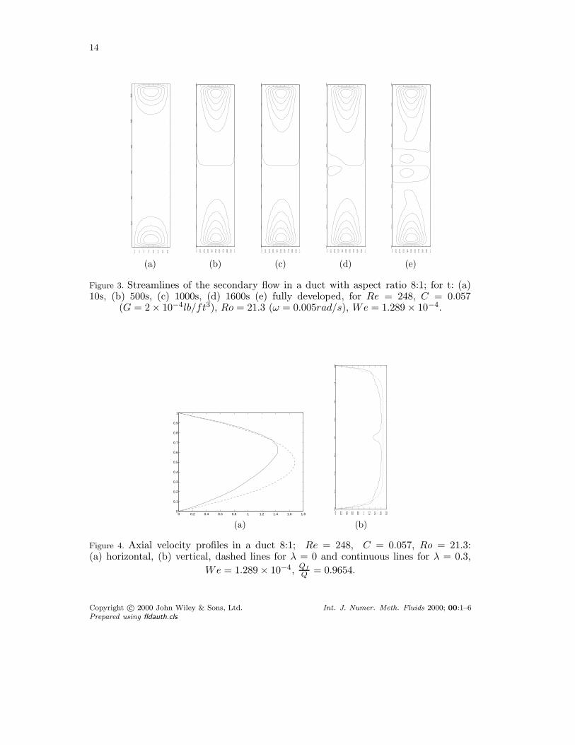
In the Figure 10, it is exhibited a transient structure of the normalized velocity of secondaryflows for the Grashof number Gr = 54330. The streamlines for the same times are presentedin the Figure 11.

It can be observed that, in the time until t = 100s (Figure 12 a), the rotation effects evenpredominate and the corresponding isotherms show that the temperature was not establishedin the domain. As time evolves, the mixed convection appears once the isotherms in (b), (c)and (d) of the Figure 12 are developing for bigger times. This type of convection influencesthe flow until the obtention of a structure flow where the recirculations, in the transversalsection of the duct, they are leaned in the lower and upper parts of the duct, giving place toanother type of recirculation that encloses almost all the transversal section. This happens inthe interval of time of 1000s to 1600s, as it can be seen in the Figures 10 c and d and Figures11 c and d. A great difference exists with the structure of a fully developed isothermal flowconsidered in the last section and showed in Figure 5.

We can also observe that the two vortex structure is broken due to the buoyancy force. Inthe Figure 11, are shown the streamlines of this flow in the transversal section. It is possibleto observe that the recirculations near the upper wall are stronger that the ones at the lowerwall.

In the Figure 13, the profiles of the longitudinal velocity of the fully developed flow canbe observed and compared with the velocity profiles without rotation. These profiles show adifferent effect than would be expected. The horizontal profile, in the center of the transversalsection (Figure 13), is greater than the velocity profile without mixed convection (Figure 6).However, at the lower and upper walls, it diminishes in the absence of the convective force,even though the flow rate of this fluid structure is 97 % in comparison to the initial outflow.

When the Grashof number is increased to Gr = 170000, the evolution of the secondary flowshows the onset of certain instabilities of the structure of the previous secondary flow. This canbe observed in Figure 14 and 15 for the streamlines. The appearance of small recirculationscan be appreciated, but almost all in the same direction. The only recirculation with oppositedirection is at the lower wall. But this one only appears at the time t = 10s; at the other timesis very weak and disappears at later times, as can be observed in the Figure 15.

Copyright c© 2000 John Wiley & Sons, Ltd. Int. J. Numer. Meth. Fluids 2000; 00:1–6Prepared using fldauth.cls

20

0.1 0.2 0.3 0.4 0.5 0.6 0.7 0.8 0.9

1

2

3

4

5

6

7

0.1 0.2 0.3 0.4 0.5 0.6 0.7 0.8 0.9

1

2

3

4

5

6

7

0.1 0.2 0.3 0.4 0.5 0.6 0.7 0.8 0.9

1

2

3

4

5

6

7

0.1 0.2 0.3 0.4 0.5 0.6 0.7 0.8 0.9

1

2

3

4

5

6

7

0 0.1 0.2 0.3 0.4 0.5 0.6 0.7 0.8 0.9 10

1

2

3

4

5

6

7

8

(a) (b) (c) (d) (e)

Figure 10. Secondary flow in a duct 8:1; for t: (a) 10s (b) 100s, (c) 500s, (d) 1600s,(e) fully developed, for Re = 260, C = 0.057 (G = 2 × 10−4lb/ft3), Ro = 21.3

(ω = 0.005rad/s), We = 2.1484 × 10−4, Gr = 54331, Pr = 8.

0 0.1 0.2 0.3 0.4 0.5 0.6 0.7 0.8 0.9 10

1

2

3

4

5

6

7

8

0 0.1 0.2 0.3 0.4 0.5 0.6 0.7 0.8 0.9 10

1

2

3

4

5

6

7

8

0 0.1 0.2 0.3 0.4 0.5 0.6 0.7 0.8 0.9 10

1

2

3

4

5

6

7

8

0 0.1 0.2 0.3 0.4 0.5 0.6 0.7 0.8 0.9 10

1

2

3

4

5

6

7

8

0 0.1 0.2 0.3 0.4 0.5 0.6 0.7 0.8 0.9 10

1

2

3

4

5

6

7

8

(a) (b) (c) (d) (e)

Figure 11. Streamlines of the secondary flow in a duct with aspect ratio 8:1 for t =(a) 10s, (b) 100s, (c) 500s, (d) 1600s (e) fully developed, for Re = 260, C = 0.057(G = 2×10−4lb/ft3), Ro = 21.3 (ω = 0.005rad/s), We = 2.1484×10−4, Gr = 54331,

Pr = 8.

Copyright c© 2000 John Wiley & Sons, Ltd. Int. J. Numer. Meth. Fluids 2000; 00:1–6Prepared using fldauth.cls

21

2 4 6 8 10 12 14 16 18

20

40

60

80

100

120

2 4 6 8 10 12 14 16 18

20

40

60

80

100

120

2 4 6 8 10 12 14 16 18

20

40

60

80

100

120

2 4 6 8 10 12 14 16 18

20

40

60

80

100

120

(a) (b) (c) (d)

Figure 12. Isotherms; for t (a) 100s (b) 500s, (c) 1600s, (d) fully developed, for Re = 260,C = 0.057 (G = 2 × 10−4lb/ft3), Ro = 21.3 (ω = 0.005rad/s), We = 2.1484 × 10−4,

Gr = 54331, Pr = 8.

0 0.5 1 1.5 2 2.5 3 3.50

0.1

0.2

0.3

0.4

0.5

0.6

0.7

0.8

0.9

1

w/Wo

x/D

0 0.5 1 1.5 2 2.5 3 3.50

1

2

3

4

5

6

7

8

w/Wo

y/D

(a) (b)

Figure 13. Axial velocity profiles (a) Horizontal, (b) vertical, for Re = 260, Ro = 21.3,We = 2.1484 × 10−4, Gr = 54331, Pr = 8, [dashed line (ω = 0), continuous line

(ω = 0.005rad/s)]. Qf

Q= 0.978, umax

wmax= 0.0456

Copyright c© 2000 John Wiley & Sons, Ltd. Int. J. Numer. Meth. Fluids 2000; 00:1–6Prepared using fldauth.cls

22

0.1 0.2 0.3 0.4 0.5 0.6 0.7 0.8 0.9

1

2

3

4

5

6

7

0.1 0.2 0.3 0.4 0.5 0.6 0.7 0.8 0.9

1

2

3

4

5

6

7

0.1 0.2 0.3 0.4 0.5 0.6 0.7 0.8 0.9

1

2

3

4

5

6

7

0.1 0.2 0.3 0.4 0.5 0.6 0.7 0.8 0.9

1

2

3

4

5

6

7

0.1 0.2 0.3 0.4 0.5 0.6 0.7 0.8 0.9

1

2

3

4

5

6

7

(a) (b) (c) (d) (e)

Figure 14. Secondary flow in a duct 8:1, para t: (a) 10s, (b) 500s, (c) 1600s, (d) 3500s,(e) fully developed, for Re = 251, Ro = 21.5 (ω = 0.005rad/s, G = 2 × 10−4lb/ft3),

We = 2.1484 × 10−4, Gr = 170000, Pr = 8.

0 0.1 0.2 0.3 0.4 0.5 0.6 0.7 0.8 0.9 10

1

2

3

4

5

6

7

8

0 0.1 0.2 0.3 0.4 0.5 0.6 0.7 0.8 0.9 10

1

2

3

4

5

6

7

8

0 0.1 0.2 0.3 0.4 0.5 0.6 0.7 0.8 0.9 10

1

2

3

4

5

6

7

8

0 0.1 0.2 0.3 0.4 0.5 0.6 0.7 0.8 0.9 10

1

2

3

4

5

6

7

8

0 0.1 0.2 0.3 0.4 0.5 0.6 0.7 0.8 0.9 10

1

2

3

4

5

6

7

8

(a) (b) (c) (d) (e)

Figure 15. Streamlines of the secondary flow in a duct with aspect ratio 8:1 em t= (a)10s, (b) 500ss, (c) 1600s, (d) 3500s (e) fully developed, for Re = 251, Ro = 21.5(ω = 0.005rad/s, G = 2 × 10−4lb/ft3), We = 2.1484 × 10−4, Gr = 170000, Pr = 8.

Copyright c© 2000 John Wiley & Sons, Ltd. Int. J. Numer. Meth. Fluids 2000; 00:1–6Prepared using fldauth.cls

23

2 4 6 8 10 12 14 16 18

20

40

60

80

100

120

2 4 6 8 10 12 14 16 18

20

40

60

80

100

120

2 4 6 8 10 12 14 16 18

20

40

60

80

100

120

2 4 6 8 10 12 14 16 18

20

40

60

80

100

120

(a) (b) (c) (d)

Figure 16. Isotherms in a duct 8:1 for t (a) 500s, (b)1600s, (c)3500s, (d) fully developed,for Re = 251, Ro = 21.5, We = 2.1484 × 10−4, Gr = 170000, Pr = 8.

0 0.5 1 1.5 2 2.5 3 3.50

0.1

0.2

0.3

0.4

0.5

0.6

0.7

0.8

0.9

1

w/Wo

x/D

0 0.5 1 1.5 2 2.5 3 3.50

1

2

3

4

5

6

7

8

w/Wo

y/D

(a) (b)

Figure 17. Axial velocity profiles in a duct 8:1, (a) Horizontal (y/D = 4), (b) vertical(x/D = 0.5), [dashed line (ω = 0), continuous line (ω = 0, 005rad/s)] for Re = 251,

Ro = 21.5, We = 2.1484 × 10−4 Gr = 170000, Pr = 8, Qt

Q= 0.9391, umax

wmax= 0.0847.

Copyright c© 2000 John Wiley & Sons, Ltd. Int. J. Numer. Meth. Fluids 2000; 00:1–6Prepared using fldauth.cls

24

In Figure 16, the isotherms were obtained for the same times as the ones for whichthe velocity fields were calculated. These isotherms are very similar to the ones of naturalconvection with ducts of high aspect ratio [8]. We can observe that, in this situation, thebuoyancy force is the predominant one and neutralizes the effects of the Coriolis force.

8. Conclusions

A numeric study has been conducted for the internal flow of a weakly viscoelastic fluid ina rotating rectangular duct subject to a bouyancy force. The numerical method of finitedifferences was employed in primitive variables with a Neumann condition for the pressureon a staggered grid.

Numerical simulations for the cases of a rotating weakly viscoelastic flow with and withoutmixed convection have been carried out by using a direct velocity-pressure algorithm whichsolves the Poisson equation for the pressure without any iteration. This equation is timedependent due to the incorporation of the velocity field through the Neumann condition forthe pressure.

Without natural convection, the numerical results for ducts with aspect ratio 2:1 and 8:1show that when the Weissenberg number increases (We > 7.4 × 10−5), the configuration ofthe secondary flow becomes contains multiple vortexes until a double vortex configuration isachieved, as predicted by Speziale [4].

For the first case, the numeric results for ducts with aspect ratio 2:1 and 8:1 show that whenthe Weissenberg number increases (We > 7.4 × 10−5), the secondary flow is restabilized to astretched double vortex configuration, which was predicted by Speziale [4].

The numerical results for the second case, with ducts of aspect ratio 8:1, show that thebouyancy forces neutralize the effects of the Coriolis force.

Special attention was given to the transient development of the structures of the fields inthis study. The reason for the study is that the literature does not contain much informationabout these cases. The numerical scheme developed in this work for a rotating flow can beemployed for larger scales in geophysical problems as well as with porous walls [12].

acknowlegdement

We thank the referees for their important comments and suggestions about this work.

Copyright c© 2000 John Wiley & Sons, Ltd. Int. J. Numer. Meth. Fluids 2000; 00:1–6Prepared using fldauth.cls

25

REFERENCES

1. J. R. Claeyssen, E. Bravo, and R. Platte, Simulation in primitive variables of incompressible flowwith pressure Neumann condition, Int.J.Numer.Meth.Fluids, (30) 1999, pp. 1009–1026.

2. P. M. Gresho, and R. L. Sani, On pressure boundary conditions for the incompressible Navier-Stokesequations, Int.J.Numer.Meth.Fluids, (7) 1987 , pp. 1111–1145.

3. H. B. Chen, K. Nandakumar, W. H. Finlay, and H. C. Ku, Three-dimensional viscous flow throughrotating channel: A Pseudospectral matrix method approach, Int.J.Numer.Meth.Fluids, (23) 1996, pp.379–396.

4. C. G. Speziale, Numerical Study of Viscous Flow in Rotating Rectangular Ducts, J. Fluid Mech, (122)1982, pp. 251–271.

5. C. G, Speziale, Numerical solution of rotating internal flows, Lect. in App.Math., AMS, (22) 1985, pp.261–288.

6. A. M. Robertson, On Viscous Flow in curved pipes of non–uniform cross-section, Int.Jour.Num.Meth.Fluids, (22) 1996, pp. 771–798.

7. R. E. Khayat, On Overstability in thermal convection of viscoelastic fluids, Developments in Non-Newtonian Flows AMD, ASME, (175) 1993, pp. 71–83.

8. Y. y. Jin, and C. F. Chen, Instability of convection and heat transfer of high Prandtl number fluids ina vertical slot, J. Heat Trans., (118) 1996, pp. 359–365.

9. C. Nonino, and G. Comini, An equal-order velocity–pressure algorithm for incompressible thermal flows,Part 1: Formulation, Num. Heat Trans., Part B, (32) 1997, pp. 1–15.

10. C. Nonino, and G. Croce, An equal-order velocity–pressure algorithm for incompressible thermal flows,Part 2: Validation, Num. Heat Trans., Part B, (32) 1997, pp. 17–35.

11. W. Liqiu, Buoyancy-force-driven transitions in flow structures and their effects on heat transfer inrotating curved channel, Int. J. Heat Mass Trans., (40-2) 1997, pp. 223–235.

12. K. T. Lee, and W. M. Yan, Mixed convection heat and mass transfer in radially rotating rectangularducts, Num.Heat Trans., Part A, (34) 1998, pp. 747-767.

13. E.Lee, Y.H. Lee, Y.T.Pai, J.P.Hsu , Flow of a viscoelastic shear-thinning fluid between two concentricrotating spheres, Chem.Eng.Sci., (57) 2002, pp. 507–514.

14. H.M. Park., S.M. Hong, J.Y. Lim,Estimation of rheological parameters using velocity measurements,Chem.Eng.Sci. 62 (2007) pp. 6806–6815.

15. Z. Yang, Large eddy simulation of fully developed turbulent flow in a rotating pipe,Int.J.Numer.Meth.Fluids, (33) 2000, pp. 681–694.

16. P. A. Govatsos, and D. E. Papantonis, A characteristic based method for the calculation of three-dimensional incompressible, turbulent and steady flows in hydraulic turbomachines and installations,Int.J.Numer.Meth.Fluids, (34) 2000, pp. 1–30.

17. P. J. Vanyo, Rotating Fluids in Engineering and Science, Dover Publications, Inc. Mineola, New York,1993.

18. J. E. Hart, Instability and secondary motion in a rotating channel flow, J. Fluid Mech, (45) 1971, pp.341–351.

19. O. Ladyzhenskaya, The Mathematical Theory of Viscous Incompressible Flow, Gordon & Breach, NewYork, 1969.

20. T. W. H. Sheu, M. M. T. Wang, and S. F. Tsai, Pressure boundary condition for a segregated approachto solving incompressible Navier–Stokes equations, Numerical Heat Transfer, Part B, (34) 1998, pp. 457–467.

21. F. H. Harlow, and J. E. Welch, Numerical calculation of time dependent viscous incompressible flowof fluid with free surface, Phys. Fluids, (8) 1965, pp. 2182–2189.

22. P. J. Roache, Computational Fluid Dynamics, Hermosa Pub., Albuquerque N M, 1982.23. W. F. Ames, Numerical Methods for Partial Differential Equations, Third ed., Academic Press, 1992.24. J. H. Ferziger, and M. Peric, Computational Methods for Fluid Dynamics, Second edition, Springer,

1999.25. S. Abdallah, Numerical solutions for the pressure Poisson equation with Neumann boundary conditions

using a non-staggered grid, Journal of Computational Physics, (70) 1987, pp. 182–192.26. B. J. Alfrink, On the Neumann Problem for the pressure in a Navier–Stokes model, Proc. 2nd Int. Conf.

on Numerical Methods in Laminar and Turbulent Flow, Venice, 1981, pp. 389–399.27. P. M. Morse, and H. Feschbach, Methods of Theoretical Physics, Part I, McGraw-Hill, 1953.28. R. Temam, Navier-Stokes Equations,Theory and Numerical Analysis, Third ed., North-Holland,

Amsterdam, 1984 (reprint AMS Chelsea Publishing, Providence, RI,2004).29. H. Yamaguchi, J. Fujiyoshi, H. Matsui, Spherical Couette flow of a viscoelastic fluid Part I:

Experimental study of the inner sphere rotation,J. Non-Newtonian Fluid Mech.,1997, (69),pp.29-46.30. J. Ferguson, and Z. Kemblowski, Applied Fluid Rheology, Elsevier Applied Science, London, 1991.

Copyright c© 2000 John Wiley & Sons, Ltd. Int. J. Numer. Meth. Fluids 2000; 00:1–6Prepared using fldauth.cls

26

31. D. D. Joseph, Fluid Dynamics of Viscoelastic Liquids, Springer-Verlag, New York, 1990.32. J. R. Claeyssen, E. Bravo, and O. Rubio, Rotating Incompressible Flow with a Pressure Neumann

Condition, Int.J.Numer.Meth.Fluids, (50) 2006, pp. 1–26

Copyright c© 2000 John Wiley & Sons, Ltd. Int. J. Numer. Meth. Fluids 2000; 00:1–6Prepared using fldauth.cls