A Contribution to the Schumpeterian Growth Theory and Empirics · A Contribution to the Schumpeterian Growth Theory and Empirics Cem Ertury Wilfried Koch z Revise and resubmit to

A Contribution to the Schumpeterian Growth

Theory and Empirics∗

Cem Ertur† Wilfried Koch ‡

Revise and resubmit to the Journal of Economic Growth

Abstract

This paper proposes an integrated theoretical and methodological framework character-ized by technological interactions to explain growth processes from a Schumpeterian per-spective. Global interdependence implied by international R&D spillovers needs to be takeninto account in the theoretical model as well as in the empirical model. The spatial econo-metric methodology is the adequate tool to empirically deal with this issue. The econometricmodel we propose includes the neoclassical growth model as a particular case. We can there-fore explicitly test the role of R&D investment in the long run growth process against theSolow growth model. Finally, the properties of our spatial econometric specification allowevaluating explicitly the impact of home and foreign R&D spillovers.

KEYWORDS: multi-country model, Schumpeterian growth, R&D spillovers, spatial econo-metrics

JEL: C31, O3, O4

∗We thank conference participants at Cambridge and Kiel for helpful comments and suggestions. We also wouldlike to thank Philippe Aghion and Richard Rogerson for their valuable comments. The usual disclaimer applies.Wilfried Koch acknowledges financial support of the CNRS-GIP-ANR “young researchers” program. WilfriedKoch and Cem Ertur acknowledge financial support from the 2006 CPER Bourgogne program (06-CPER-189-01and GIP-ANR 4010). The usual disclaimer applies.†LEO, Universite d’Orleans, France. E-mail: [email protected]‡Universite du Quebec a Montreal (UQAM) and CIRPEE. E-mail: [email protected], corresponding

author.

1

“A generally unexplored possibility for studying cross-section dependence in growth (and

other contexts) is to model these correlations structurally as the outcome of spillover effects.”

(Durlauf, Johnson and Temple, 2005)

1 Introduction

Is the real world growth process better explained by the neoclassical or the Schumpeterian growth

theories? To the best of our knowledge, this question has not found a direct, clear and convincing

answer in the growth literature. For the neoclassical growth model, factor accumulation and

exogenous technological progress are the key determinants of the growth process. In contrast,

for the Schumpeterian growth model, the growth process is based on endogenous profit driven

knowledge accumulation and diffusion. The modeling strategy and econometric methodology

traditionally used in the literature to estimate those models cannot help to discriminate between

the two competing theories. On the one hand, empirical evidence found using the neoclassical

growth model has often been interpreted to cast some doubt on endogenous growth models as

also underlined by Howitt (2000). However, this cannot be considered as direct evidence against

endogenous growth models. On the other hand, there seems to be a growing consensus view

that technology adoption should be considered as endogenous in order to think about why the

poorest countries in the world remain so poor. This view needs to be confronted to data using

the appropriate econometric methodology and tested.

Our main contribution is to cast both models in an integrated theoretical and methodological

framework and to propose a simple test of a generalized version of the multi-country Schumpete-

rian growth model based on the one elaborated by Howitt (2000) versus a multi-country Solow

growth model (Solow, 1956) with imperfect technological interdependence similar to that pro-

posed by Ertur and Koch (2007). Actually we show that the latter is nested in the former, once

world-wide technological interdependence, well documented in the empirical literature (Keller,

2004), is explicitly modeled and estimated using the overlooked methodological tools of spatial

econometrics (Anselin, 1988). Therefore, our generalized model can be interpreted as a Schum-

peterian extension of the Solow growth model since in addition to factor accumulation, we show

that innovation caused by R&D investment plays a major role in explaining the growth pro-

cess. Our model includes both determinants, with technological diffusion occurring concretely

between pairs of countries, human capital reflecting absorptive capacity along the lines of Nelson

and Phelps (1966), and physical capital playing the usual role. More specifically, we show that

when the R&D expenditures have no effect on the growth rate of technology, our multi-country

Schumpeterian growth model reduces to the multi-country Solow growth model. The implied

constraints may be easily tested and are actually rejected in our sample. Our integrated multi-

country Schumpeterian growth model appears therefore as the best explanation of the growth

process.

Explicit modeling of technological interdependence is then crucial to challenge the fundamen-

tal question raised in the growth literature and to elaborate a completely integrated theoretical

2

as well as empirical framework. This is our specific contribution regarding the model proposed by

Howitt (2000), which is, in our opinion, incomplete and misspecified since complex interactions

between countries are overlooked or oversimplified.1

Traditionally, empirical growth papers structurally derive econometric reduced forms from

the neoclassical growth model along the lines of Mankiw et al. (1992), since it has some suitable

properties, which facilitate its econometric estimation. Indeed, all countries have an identical

long run growth rate implying that their long run growth paths are parallel. Another salient

characteristic of this model is the fact that all countries have access to the same pool of knowledge

(Mankiw, 1995). In contrast, earlier endogenous growth models do not share those theoretical

properties and face some problems.

From the empirical perspective, Mankiw et al. (1992) argue that the neoclassical growth

model with exogenous technological progress and diminishing returns to capital explains most

of the cross-country variation in per worker output. Evidence of β-convergence in growth re-

gressions (Barro and Sala-i-Martin, 2004) is often claimed to be consistent with neoclassical

theory but not with endogenous growth theory. Evans (1996) shows that the dispersion of per

capita income across advanced countries has exhibited no tendency to rise over the postwar era,

as would be predicted by some endogenous growth models; instead, these countries have been

converging to parallel growth paths of the sort implied by the neoclassical growth model with a

common world technology.

Another major problem faced by endogenous growth models is that they are difficult to

estimate since they imply that growth rates at steady state are endogenously determined by the

level of income or by the current out-of steady state growth rate. Steady-state growth rates are

therefore specific to each country and should be simultaneously estimated. In the neoclassical

framework, this variable is assumed exogenous and identical for each country. Some authors, like

Dinopoulos and Thomson (2000) for instance, propose to use simultaneous non-linear systems of

equations to estimate Romer-Jones type of models (Romer, 1990; Jones, 1995), whereas Aghion

and Howitt (1998) or Howitt (2000) propose to consider international diffusion of knowledge in

the Schumpeterian growth model in order to estimate endogenous growth models. The latter

approach has the interesting propriety to imply parallel long run growth paths, just like the

neoclassical growth model, along with intentional actions taken by economic agents who respond

to market incentives in order to accumulate new technology.

Therefore, in order to formulate an empirically tractable endogenous growth model encom-

passing the Solow model, we not only take Robert Solow seriously but we also take Philippe

Aghion and Peter Howitt seriously. As a starting point, we consider the multi-country Schum-

peterian growth model elaborated by Aghion and Howitt (1998) and Howitt (2000). Because of

technology transfer, countries converge at long run to the same growth rate, which is the world

growth rate. Therefore we can study the empirical implications of this model as we would do for

the neoclassical growth model. However, in the neoclassical growth model, where each country is

1However, we acknowledge that Aghion and Howitt were aware of the limitations of the Howitt model (seefootnote 23, p. 421, 1998).

3

assumed to have the same technology and the same exogenous technical progress, the differences

between countries around the technology path are random. In contrast, in the Schumpeterian

growth model, where R&D expenditures are motivated by profit, the distribution of countries’

technology depends on their R&D expenditures. Our contribution is to explicitly augment the

research productivity function of endogenous growth models by adding a general process of

technological interdependence as the one proposed by Ertur and Koch (2007). We assume that

the productivity of R&D expenditures is low when countries are close to their own technology

frontier and is high when countries are far from their own technology frontier, as also recently

proposed by Aghion and Howitt (1998), Howitt and Mayer-Foulkes (2005) or Acemoglu et al.

(2006) in order to take into account the “advantage of backwardness” (Gerschenkron, 1952) con-

ferred on technological laggards. We show that this assumption leads to a spatial econometric

reduced form which is somewhat latent and not fully exploited in Aghion and Howitt (1998)

or Howitt (2000). Indeed, the global interdependence implied by international R&D spillovers

needs to be taken into account in the theoretical model as well as in its empirical counterpart.

The empirical specification proposed by Aghion and Howitt (1998) or Howitt (2000) appears

then to be misspecified since it omits this interdependence whereas it is fundamental in their

theoretical model: their reduced econometric form does not capture all the rich qualitative and

quantitative implications of the multi-country Schumpeterian growth model.

The modeling strategy proposed in this paper has therefore the following four main ap-

pealing characteristics. First, our modeling strategy is to work with multi-country models in

growth theory in order to capture the implications of technological interdependence. Indeed,

as underlined by Behrens and Thisse (2007, p.461) “In many scientific fields, the passage from

one to two dimensions raises fundamental conceptual difficulties.” The reason for this is that

when there are just two countries, there is only one way in which these countries can interact,

namely directly; whereas with three countries, there are two ways in which these countries can

interact, namely directly and indirectly. In other words, in multi-country systems the so-called

“three-ness effect” enters the picture and introduces complex feedbacks into the models, which

significantly complicates the analysis. Although the two countries modeling strategy gives clear

economic intuition about economic growth, it cannot capture these effects and cannot imply a

relevant econometric reduced form in a real world composed by several interdependent coun-

tries. Dealing with this world-wide technological interdependence in growth models using a

multi-country framework constitutes one of the main objective in this paper.

Second, we derive econometric reduced forms which take into account interdependence be-

tween countries, challenging the so-called exchangeability hypothesis (Brock and Durlauf, 2001).

Spatial econometric specifications are indeed derived structurally from these multi-country

growth models and we show that they are the most appropriate specifications to deal with

the kind of technological interdependence process we propose. As already mentioned, let us un-

derline once more that those specifications are exactly designed to estimate models in implicit

form avoiding the need to solve for their explicit form before estimation. In the last two decades,

4

several papers drew attention to potential cross section error correlation in growth models.2 Let

us mention just a few of them. As noted by De Long and Summers (1991, p.487): “it is difficult

to believe that Belgian and Dutch or US and Canadian economic growth would ever significantly

diverge, or that substantial productivity gaps would appear within Scandinavia”. They also un-

derline the fact that, in the growth context, failure to account for cross section dependence can

lead to incorrect calculation of standard errors and hence, incorrect inferences. Mankiw (1995)

points out that multiple regression in the standard framework treats each country as if it were

an independent observation. Temple (1999), in his survey of the new growth evidence, draws

attention to error correlation and regional spillovers though he interprets these effects as mainly

reflecting an omitted variable problem. Conley and Ligon (2002) and Moreno and Trehan (1997)

use reduced form spatial econometric specifications and geographic and/or economic distances

to underline the impact of cross-country spillovers on growth processes. More recently, Klenow

and Rodriguez-Clare (2005) underline that national growth rates appear to depend critically on

the growth rates and income levels of other countries, rather than just on any one country’s own

domestic investment rates in physical and human capital. They present stylized facts reflecting

world-wide interdependence, which could be explained by cross-country externalities.

As underlined by Brock and Durlauf (2001) and Durlauf et al. (2005), the typical cross-

country growth regressions used in the literature raise different kind of problems both from the

theoretical and methodological points of view. More precisely, they categorize these problems

in three groups: open-endedness of theories, parameter heterogeneity, correlation and causal-

ity. They subsume these problems within the concept of exchangeability, which can be loosely

defined as interchangeability of the standard growth regression errors across observations: “dif-

ferent patterns of realized errors are equally likely to occur if the realizations are permuted across

countries. In other words, the information available to a researcher about the countries is not

informative about the error terms.” (Durlauf et al., 2005, p. 36). Most of the criticisms of

standard growth regressions can be interpreted as a violation of the implicit exchangeability

hypothesis traditionally made to estimate growth regressions. It is the case of omitted variables

and parameter heterogeneity problems often raised in the literature. Presence of cross section

correlation in growth regressions as documented in the literature also constitutes a major vi-

olation of the exchangeability hypothesis. In other words, countries cannot be considered as

“isolated islands” (Quah, 1996). As also underlined by Ertur and Koch (2007), although largely

admitted, world-wide interdependence has not yet been modeled, to the best of our knowledge,

from a theoretical perspective so as to be structurally integrated in an endogenous growth model

that yields an estimable reduced form econometric specification. Ertur and Koch (2007) struc-

turally integrate technological interdependence in the neoclassical and “AK” growth models,

but their model does not imply endogenous growth. That is therefore the second main objective

of this paper.

Third, using our multi-country modeling strategy and implied spatial econometric reduced

2See Le Gallo and Rey (2008) for a recent review.

5

forms, we show that the multi-country Schumpeterian growth model, naturally generates inter-

national knowledge spillovers. More precisely, our theoretical and empirical growth models are

able to take into account both direct and indirect interactions between countries in contrast to

the two countries modeling strategy or the empirical literature devoted to international R&D

spillovers. Indeed, since they estimate econometric specifications elaborated from the two coun-

tries model of Grossman and Helpman (1991), the seminal papers of Coe and Helpman (1995)

and Coe et al. (1997) consider only direct effects of international R&D diffusion on Total Factor

Productivity. Lumenga-Neso et al. (2005) recently underline the importance of indirect effects,

but their empirical specification is not a reduced form of a theoretical model and, in our opinion,

they do not use the most appropriate estimation method. Actually, their econometric specifica-

tion is inherently spatial and needs to be estimated using the spatial econometric methodology.

In contrast, our spatial econometric specification devoted to international R&D spillovers is the

reduced form of the multi-country Schumpeterian growth model. It encompasses the findings of

all those empirical papers since we simultaneously consider in our analysis intra-OECD R&D

spillovers as Coe and Helpman (1995), North-South R&D spillovers as Coe et al. (1997) and

indirect effects as Lumenga-Neso et al. (2005). Four, convergence clubs and interdependence

between countries are closely linked. Galor (1996, p.1056) identifies three types of convergence

defined as follows: (i) the absolute convergence hypothesis where per capita incomes of coun-

tries converge to one another in the long-run independently of their initial conditions, (ii) the

conditional convergence hypothesis where per capita incomes of countries that are identical in

their structural characteristics converge to one another in the long-run independently of their

initial conditions and (iii) the club convergence hypothesis (polarization, persistent poverty and

clustering) where per capita incomes of countries that are identical in their structural character-

istics converge to one another in the long-run provided that their initial conditions are similar

as well or in other words countries converge to one another if their initial conditions are in the

basin of attraction of the same steady-state equilibrium. Durlauf and Quah (1999) identify,

using the Lucas (1993) model, an another form of club convergence, which is not directly linked

with initial conditions or non-linearities. Indeed, interdependence between countries can gener-

ate convergence clubs. In Lucas (1993), where human capital generates international spillovers,

countries converge to the same steady state if they have access to the same average world human

capital stock whereas they converge to different steady states when they have access to different

average world human capital stocks. We can therefore define an another type of club conver-

gence as follows: the club convergence hypothesis where per capita incomes of countries converge

to one another in the long-run provided that their access to foreign technology is similar. For

instance, using this definition, the neoclassical growth model does not imply club convergence

since all countries have access to the same stock of knowledge, whereas the multi-country model

we develop in this paper implies this sort of clubs since we explicitly introduce technological in-

terdependence between countries. Moreover, from the empirical point of view, club convergence

implies parameter heterogeneity in econometric specifications (Durlauf et al. 2005). As already

mentioned, economic growth models including technological interdependence between countries

6

imply spatial econometric reduced forms. These specifications are estimated using an implicit

form so that, even if we consider homogenous structural parameters for the production function

or the impact of externalities, the local impact of each exogenous variable is specific to each

country when we formulate them in explicit form.

The rest of the paper is organized as follows. Section 2 presents the multi-country Schumpeterian

growth model. Section 3 introduces our technological diffusion process. Section 4 derives the

steady state of per worker income. Section 5 is devoted to the spatial econometric reduced form

of the multi-country Schumpeterian growth model and the estimation method we use. Section

6 describes the data set and the interaction or spatial weights matrices used in the estimation.

Section 7 presents the econometric results and finally Section 8 concludes.

2 Physical capital accumulation in the multi-country Schum-

peterian growth model

2.1 Hypotheses

Production relations Let us consider as a starting point the multi-country Schumpeterian

growth model elaborated by Aghion and Howitt (1998) and Howitt (2000). Consider a single

country in a world economy with n different countries. There is one final good, produced

under perfect competition by labor and a continuum of intermediate products, according to the

production function:

Yi(t) = Qi(t)α−1

∫ Qi(t)

0Ai(v, t)xi(v, t)

αLi(t)1−αdv (1)

where Yi(t) is the country’s i gross output at date t, Li(t) = Li(0)enit is the flow of raw labor

used in production and ni its rate of growth, Qi(t) measures the number of different intermediate

products produced and used in the country i at date t, xi(v, t) is the flow output of intermediate

product v ∈ [0, Qi(t)] used at date t and Ai(v, t) is a productivity parameter attached to the

latest version of intermediate product v. As also underlined by Howitt (2000, p.831), in order to

underline technology transfer as the main connection between countries, we assume that there is

no international trade in goods or factors. Each intermediate product is specific to the country

in which it is used and produced, although, as we will see, the idea for how to produce it can

originates in other countries.

We assume that labor supply and population size are identical. They both grow exogenously

at the fixed proportional rate ni. The form of the production function, that is the presence

of the term Qi(t) dividing the labor, ensures that growth in product variety does not affect

aggregate productivity. Therefore, we suppose as Aghion and Howitt (1998) and Howitt (2000)

that the number of products grows as result of serendipitous imitation, not deliberate innovation.

Imitation is limited to domestic intermediate products; thus each new product will have the same

productivity parameter as a randomly chosen existing product within the country. Each agent

7

has the same propensity to imitate ξ > 0, which we assume identical for each country i. Thus

the aggregate flow of new products is: Qi(t) = ξLi(t). Moreover, since the population growth

rate is constant, the number of workers per product li(t) ≡ Li(t)/Qi(t) converges monotonically

to the constant:

li = ni/ξ (2)

Assume that this convergence has already occurred, so that: Li(t) = liQi(t) for all t. The form

of the production function (1) ensures that growth in product variety does not affect aggregate

productivity. This and the fact that population growth induces product proliferation guarantee

that the model does not exhibit the sort of scale effect that Jones (1995) argues is contradicted

by postwar trends in R&D spending and productivity.

At symmetric equilibrium, we have: xi(t) = ki(t)li(t) with: ki(t) ≡ Ki(t)/(Ai(t)Li(t)) the

capital stock per effective worker, Ki(t) =∫ Qi(t)0 Ki(v, t)dv represents the equality of the total de-

mand and given supply of capital, and Ai(t) ≡ 1Qi(t)

∫ Qi(t)0 Ai(v, t)dv is the average productivity

parameter across all sectors. Substitution of xi(t) at symmetric equilibrium into the produc-

tion function (1) shows that output per effective worker is given by the familiar intensive-form

production function:

yi(t) = ki(t)α (3)

with yi(t) ≡ Yi(t)/(Ai(t)Li(t)) the level of production per effective worker.

The monopolist firms’ problem Final output can be used interchangeably as a consumption

or capital good, or as an input to R&D sector. Each intermediate product is produced using

capital, according to the production function:

xi(v, t) = Ki(v, t)/Ai(v, t) (4)

where Ki(v, t) is the input of capital in sector v. Division by Ai(v, t) indicates that successive

vintages of the intermediate product are produced by increasingly capital-intensive techniques.

Innovations are targeted at specific intermediate products. Each innovation creates an improved

version of the existing product, which allows the innovator to replace the incumbent monopolist

until the next innovation in that sector. The cost function of the monopolist firm is given by:

(ri(t) + δ)Ki(v, t) = (ri(t) + δ)Ai(v, t)xi(v, t) (5)

where (ri(t) + δ) is the cost of the capital, that is the rate of interest ri(t) and δ is the fixed

rate of depreciation. The price schedule, or the inverse demand function pi(v, t), facing the

monopolist is: pi(v, t) = αAi(v, t)xi(v, t)α−1li(t)

1−α. The monopolist firm therefore maximizes

the following profit function:

maxπi(v, t) = pi(v, t)xi(v, t)− (ri(t) + δ)Ai(v, t)xi(v, t) (6)

8

With the properties of the cost and the inverse demand functions, we can resolve the monopolist

maximization problem to obtain the equilibrium interest rate:

ri(t) = α2ki(t)α−1 − δ (7)

Substituting this result in the profit function, we obtain πi(v, t) = Ai(v, t)πili(t) with πi(ki(t)) ≡α(1− α)ki(t)

α.

2.2 Vertical innovations

Poisson arrival rate Improvements in the productivity parameters of intermediate products

come from R&D activities. This sector uses only the final good as production factor. The

Poisson arrival rate of vertical innovations in any sector is:

φi(t) = λiκi(t)φ (8)

with 0 ≤ φ ≤ 1 the parameter measuring the impact of R&D expenditure on Poisson arrival

rate, λi > 0 the parameter indicating the productivity of vertical R&D, κi(t) =Si,A(t)

Qi(t)Ai(t)max

is the productivity-adjusted expenditure on vertical R&D in each sector.3 We deflate R&D

expenditures in each sector (Si,A(t)/Qi(t)) by Ai(t)max the leading-edge productivity parameter

to take into account the force of increasing complexity; as technology advances, the resource cost

of further advances increases proportionally. This hypothesis prevents growth from exploding

as the amount of capital available as an input to R&D grows without bound. The leading-edge

technology is the maximal value of Ai(v, t) at date t defined as:

Ai(t)max ≡ max {Ai(v, t); v ∈ [0, Qi(t)]} (9)

Value of an innovation Define the value of an innovation by Vi(t) and the productivity-

adjusted value of an innovation by: vi(t) ≡ Vi(t)Ai(t)max

. The value of an innovation is given by:

Vi(t) =

∫ ∞t

e−∫ τt (ri(s)+φi(s))dsπi(τ)dτ (10)

Accordingly the value of a vertical innovation at date t is the present value of the future profits

to be earned by the incumbent before being replaced by the next innovator in that product.

Noting that a firm which innovates at date t has a productivity Ai(v, τ) = Ai(t)max for all τ > t

until replacement by another which innovates. Introducing equation describing the profit, we

3As denoted by Aghion and Howitt (1998), since the prospective payoff is the same in each sector, we dividetotal R&D expenditures in country i by the number of sectors in this country, so that R&D expenditures areidentical in each sector.

9

can rewrite (10) as follows:

vi(t) =

∫ ∞t

e−∫ τt (ri(s)+φi(s))dsliπi(ki(τ))dτ (11)

Deriving with respect to time, we obtain:

vi(t)

vi(t)= ri(t) + φi(t)−

liπi(ki(t))

vi(t)(12)

This equation is the classical research-arbitrage equation. The profit of private firm v in research

sector, denoted by πi,A(v), is given by:

πi,A(v) = λiκi(t)φ Si,A(v, t)

Si,A(t)/Qi(t)Vi(t)− Si,A(v, t) (13)

with λiκi(t)φ the Poisson arrival rate, Si,A(v, t) is the quantity of final good invested in R&D

by the firm v, Si,A(t)/Qi(t) is the quantity of final output invested by all firms in this sector

representing here negative externalities due to duplication or overlap research. The marginal

cost is supposed equal to one without loss in generalities. The first order condition of the profit

maximization gives:dπi,A(v)

dSi,A(v, t)= 0⇔ 1 = λi

κi(t)φ

Si,A(t)/Qi(t)Vi(t) (14)

that is the value of one innovation:

vi(t) =1

λiκi(t)

1−φ (15)

Taking the derivative with respect to time in both sides and rearranging terms, we obtain the

differential equation describing the evolution of the amount of final good invested in R&D sector:

vi(t)

vi(t)= (1− φ)

κi(t)

κi(t)⇔ κi(t)

κi(t)=

1

1− φ

[ri(t) + λiκi(t)

φ − λiκi(t)φ−1liπi(ki(t))]

(16)

Growth of the leading-edge parameter Growth in the leading-edge parameter occurs as a

result of the knowledge spillovers produced by vertical innovations. Following Caballero and Jaffe

(1993), Aghion and Howitt (1998, 1999) and Howitt (1999, 2000) assume that Ai(t)max grows at

a rate proportionate to the aggregate rate of vertical innovations. The factor of proportionality,

which is a measure of the marginal impact of each innovation on the stock of public knowledge, is

assumed to equal σQi(t)

> 0. We divide by Qi(t) to reflect the fact that as the economy develops

an increasing number of specialized products, an innovation of a given size with respect to any

given product will have a smaller impact on the aggregate economy. The rate of technological

progress equals:

gi(t) ≡Ai(t)

max

Ai(t)max=

σ

Qi(t)Qi(t)λiκi(t)

φ = σλiκi(t)φ (17)

10

with σQi(t)

the factor of proportionality, Qi(t) is the number of horizontally differentiated goods,

λiκi(t)φ is the rate of innovation for each product, Qi(t)λiκi(t)

φ is the aggregate flow of inno-

vation. Therefore, the rate of technological progress equals to the aggregate flow of innovations

times the factor of proportionality.

Relation of proportionality between the leading-edge and average parameter Each

innovation replaces a randomly chosen Ai(v, t) with the leading-edge technology parameter

Ai(t)max. Since innovations occur at the rate λiκi(t)

φ per product and the average change

across innovating sectors is Ai(t)max −Ai(t), we have:

dAi(t)

dt= λiκi(t)

φ(Ai(t)max −Ai(t)) (18)

As Aghion and Howitt (1998), we can show that the ratio Ai(t)max

Ai(t)converges asymptotically to

1 + σ. Thus we assume that Ai(t)max = Ai(t)(1 + σ) for all t, so that the rate of growth of the

average productivity parameter Ai(t) will also given by that of Ai(t)max in equation (17).

2.3 Physical capital accumulation and steady state analysis

The law of motion of aggregate physical capital is given by the fundamental dynamic equation

of Solow as in the neoclassical growth model:

˙ki(t) = sK,iki(t)

α − (ni + gi(t) + δ)ki(t) (19)

where sK,i is the investment rate and δ is the rate of depreciation of physical capital assumed

identical for each country.

In this section, we first consider that each economy is independent from others. The evolution

of economy i is described by the following system of differential equations:

˙ki(t) = sK,iki(t)

α − (ni + σλiκi(t)φ + δ)ki(t) (20)

κi(t) =κi(t)

1− φ

[ri(t) + λiκi(t)

φ − λiκi(t)φ−1liπi(ki(t))]

(21)

with: gi(t) = σλiκi(t)φ.

At steady state, we have˙ki(t) = κi(t) = 0 and g?i = σλiκ

?φi . The equation describing the

accumulation of physical capital becomes in implicit form:

k?αi =sK,i

ni + σλiκ?φi + δ

(22)

We note that an increase of research increases the rate of technological progress at steady state

and decreases the ratio capital-output at steady state and therefore the per effective worker

physical capital at steady state. We obtain the decreasing curve (K).

11

For the equation describing the accumulation of R&D, we have at steady state in implicit

form the arbitrage equation of the Schumpeterian growth model:

1 = λiκ?φ−1i

πi(k?i )li

r?i + λiκ?φi

(23)

We obtain the increasing curve (A). It is increasing since when the per worker physical capital

increases, the profit of firms increases and the marginal revenue decreases so that research

expenditures need to increase in order to maintain equilibrium in equation (23).

——————————————————————-

Figure 1 around here

——————————————————————-

We represent these curves (K) and (A) in the upper right part of Figure 1. It represents

the interaction between neoclassical growth model and Schumpeterian growth model of Aghion

and Howitt (1992). Indeed, in the lower right part of Figure 1 we represent the neoclassical

growth model. The only difference with the well-known graph associated with this model,

is the fact that the line ni + gi(t) + δ moves up until the steady state is reached. In fact the

effective depreciation rate of capital depends on technology rate of growth which is endogenously

determined by research investment. We represent this Schumpeterian part of the model in the

upper left part of Figure 1, with the rate of growth of technology which depends on research

investments κi(t). The function is increasing and concave. At steady state, the line representing

the effective rate of depreciation is fixed and we can determine all variables at their steady state

values.

The classical comparative statics in the Schumpeterian growth literature leads to the follow-

ing Proposition:

Proposition 1 The country i’s steady state growth rate value (g?i ) positively depends on its

investment rate (sK,i) and the productivity of its research sector (λi). It depends negatively on

the depreciation rate of physical capital (δ).

Indeed, an increase of the research productivity λi makes research more productive which directly

induces an increase of the growth rate. However, we can note that per effective worker physical

capital decreases, since the curve (A) moves up in the upper right part of Figure 1, and the line

representing the effective depreciation rate of physical capital moves up too. An increase of the

investment rate moves up the curve in the lower right part of Figure 1, and the curve (K) in the

upper right part of Figure 1. As we showed, the profit of intermediate firms depends positively

on accumulated per effective worker physical capital. Therefore, the devoted resources to the

research sector increase and the growth rate increases. In contrast, the accumulated per effective

worker physical capital decreases when the depreciation rate of the physical capital increases so

that the growth rate decreases.***

12

3 International technological diffusion and the multi-country

Schumpeterian growth model

Let us consider now the multi-country Schumpeterian growth model. In order to introduce

technological diffusion in the Schumpeterian growth model, we assume that this productivity

parameter is defined as follows:

λi = λn∏j=1

(Aj(t)

Ai(t)

)γivij(24)

We therefore suppose that R&D productivity is a negative function of the technological gap of

country i with respect to its own technological frontier. This technological frontier is defined

as the geometric mean of knowledge levels in all countries denoted by Aj(t), for j = 1, ..., n.

It is specific to each country because of the vij parameters, which model the specific access of

the country i to the accumulated knowledge of all other countries. The general specification

proposed in this paper encompasses particular cases generally found in the literature like the

world or global technological leader (Benhabib and Spiegel, 1994, 2005; or Nelson and Phelps,

1966). We assume that the interaction terms vij are non negative, finite and non stochastic. We

also assume that∑n

j=1 vij = 1 for i = 1, ..., n to ensure convergence to parallel growth paths.

The parameter γi > 1 measures the absorption capacity of country i which is assumed a function

of its human capital stock as: γi = γHi, with γ < 1. Introducing equation (24) into the growth

rate of the average accumulated knowledge in country i, we have:

gi ≡Ai(t)

Ai(t)= λσκi(t)

φn∏j=1

(Aj(t)

Ai(t)

)γivij(25)

The idea developed here is very simple. We assume that each country has a technological frontier

defined in the last term of equation (25). The gap with respect to this specific technological

frontier determines the research productivity of a given country i. Indeed, the farther away a

country is from its own technological frontier the higher is its productivity in the research sector

because it can beneficiates from the accumulated knowledge in other countries. This hypothesis

can also be interpreted as international spillovers effect or as spatial externalities (Ertur and

Koch, 2007). Therefore, the closer country i is to its own technological frontier the more it is

difficult to copy foreign technology and the lower is its research productivity λi. In contrast,

the farther the country i is from its own technological frontier the more it beneficiates from

foreign technology to innovate and the higher is its research productivity. The distance with

respect to countries’ own technological frontier depends on the resources devoted to the research

sector κi(t). At steady state, all countries have constant rates of growth of their key variables,

therefore the gap with respect to their own frontier is constant and steady state occurs only if

all countries have identical growth rates, or in other words, if all countries converge to parallel

long ways of growth. At steady state, we have: g?i = gw for each country i where gw is the

13

steady state growth rate or the world growth rate. It is defined as follows:4

gw = λσκφi

n∏j=1

(AjAi

)γivijfor i = 1, ..., n (26)

Each country has the same steady state growth rate because of the inverse relation between the

resources devoted to the research sector and the productivity parameter λi. More precisely, a

country which has high expenditures in the R&D sector is close to its own technological frontier

and therefore its research productivity λi is low. In contrast, a country, which has low expendi-

tures in the R&D sector is far away from its own technology frontier and its research productivity

is high. The effect of technology diffusion on research productivity implies convergence to the

same growth rate and parallel growth paths at long run.

Although Aghion and Howitt (1998) specify a similar function, they assume that each country

has the same technological frontier since each country diffuses the same quantity of knowledge to

all other foreign countries, that is: vij = vj for each country. In their model, the technological

frontier is therefore global and not local or specific to each country as we assume. For this

reason, as we will show, the interdependence pattern can be thrown in the constant term of

their empirical specification, thus preventing full exploitation of some fundamental theoretical

and econometric implications of their theoretical model. In our model, we generalize their

approach by assuming a richer structure of interdependence between countries. Their model is

then just a particular case of ours. Moreover, as we will discuss below, we use the fact that

the interaction matrix with general term vij can be decomposed in order to model North-South

R&D diffusion. This allows then for clubs to emerge.

Recall that: κi =SA,i

QiAmaxi=

SA,iYi

YiLi

LiQi

1(1+σ)Ai

= sA,iyiniξ

1(1+σ)Ai

, where sA,i =SA,iYi

is the

investment rate in the R&D sector. Defining home technological access as: vii ≡ γi−1γi

< 1, for

i = 1, ..., n, we have:

gw =σλ

((1 + σ)ξ)φsφA,iy

φi n

φi A−φ−1i

n∏j 6=i

Aγivijj (27)

Taking logarithms of equation (27), we rewrite the obtained equation as:

lnAi =1

1 + φln

σλ

gw((1 + σ)ξ)φ+

φ

1 + φ(ln si,A + lnni + ln yi) (28)

+γHi

1 + φ

n∑j 6=i

vij lnAj

This equation shows explicitly that the knowledge accumulated in one country depends on the

knowledge accumulated in other countries. Our multi-country Schumpeterian growth model im-

plies technological interdependence between countries, therefore each country cannot be analyzed

as an independent observation. At this step, assuming that each country diffuses identically,

4At this step, all variables are defined at steady state, we therefore drop the time reference.

14

that is vij = vj for j = 1, ..., n and γi = γ for i = 1, ..., n, Aghion and Howitt (1998) consider

the last term of equation (29) as a constant. In contrast, we propose a richer interdependence

scheme, rewrite equation (29) in matrix form to obtain:

A =1

1 + φln

σλ

gw((1 + σ)ξ)φ1I(n,1) +

φ

1 + φ(sA + y + n) +

γ

1 + φWA (29)

where A is the (n×1) vector of the logarithms of average technological progress levels, 1I(n,1) the

(n×1) vector of 1, y the (n×1) vector of the logarithms of per worker income levels, sA the (n×1)

vector of the logarithms of the investment rates devoted to the research sector and n the (n×1)

vector of the logarithms of working-age population rates of growth. W is the (n×n) interaction

matrix defined as W = diag[Hi ]V, where diag[Hi ] is the diagonal matrix of human capital stocks

and V is the matrix collecting the interaction terms vij for i 6= j given that vij = 0 if i = j.

Note that, by definition, W is not row normalized. Note also that, by definition, the elements

of W are nonnegative. We can resolve this equation for A, if(I− γ

1+φW)

is non singular, that

is to say if γ1+φ 6= 0 and if

∣∣∣ γ1+φ

∣∣∣ ≤ 1min(l,c) where l = maxi

∑j wij and c = maxj

∑iwij :

A =1

1 + φ

(I− γ

1 + φW

)−1(ln

σλ

gw((1 + σ)ξ)φ1I(n,1)

)+

φ

1 + φ

(I− γ

1 + φW

)−1(sA + y + n) (30)

This relation shows that the level of average technology depends not only on the R&D expendi-

tures in the home country i but also on the R&D expenditures in foreign countries j = 1, ..., n.

The impact of foreign R&D expenditures depends on the vij parameters reflecting interactions

between country i and all other countries, and on the human capital stock Hi of the receiving

country i reflecting its absorption capacity.

4 Steady state of per worker income

Rewriting the production function in matrix form: y = A + α1−αSK, where SK is the (n × 1)

vector of the logarithms of the investment rates divided by the effective rates of depreciation

of physical capital, replacing A from equation (30) in the production function and rearranging

terms, we obtain:

y =

(ln

σλ

gw((1 + σ)ξ)φ

)1I(n,1) + φ(sA + n) +

α(1 + φ)

1− αSK −

αγ

1− αWSK + γWy (31)

15

or for a country i:

ln yi = lnσλ

gw((1 + σ)ξ)φ+ φ(ln sA,i + lnni) +

α(1 + φ)

1− αln

sK,ini + gw + δ

− αγHi

1− α

n∑j 6=i

vij lnsK,j

nj + gw + δ+ γHi

n∑j 6=i

vij ln yj (32)

This equation shows that the level of per worker income at steady state depends positively

on the same levels in other countries. It is therefore an implicit equation. The resolution of

this equation for yi implies rewriting it in an explicit form. We can then study the signs and

quantify the effects of each variable on the level of the country i’s steady state value of per

worker income.5

Proposition 2 (Effect of investment rates in physical capital) The value of per worker

income of country i at steady state depends positively on its own investment rate in physical

capital (sK,i) and positively on the investment rates in physical capital in foreign countries (sK,j

for j = 1, ..., n and j 6= i). The elasticities of the country i’s value of per worker income at

steady state with respect to its own investment rate is:

ΞsK,ii =

α(1 + φ)

1− α+

αφ

1− α

∞∑r=1

γri v(r)ii > 0 (33)

and with respect to the investment rate in the country j is:

ΞsK,ji =

αφ

1− α

∞∑r=1

γri v(r)ij > 0 for j = 1, ..., n, j 6= i (34)

Our multi-country Schumpeterian growth model has the same qualitative predictions as the

neoclassical growth model about the effect of investment rates in the physical capital sector.

However, because of technological interdependence and the interaction between research ex-

penditures and physical capital accumulation, this model has different quantitative predictions.

First, we note that if φ = 0, that is when R&D expenditures have no effect on growth, the elas-

ticities reduce to that of the Solow growth model: ΞsK,ii = α

1−α and ΞsK,ji = 0, for j = 1, ..., n.

If γi = 0, that is in the absence of technological interdependence, the impact of the investment

rate in physical capital is higher than in the Solow growth model: α(1+φ)1−α > α

1−α . In fact,

if the country i has an higher investment rate in physical capital, the profits of intermediate

firms increase and the research becomes more attractive. An increase of research expenditures

increases the average productivity of the country i and therefore its steady state per worker

income value. We note finally that the multi-country Schumpeterian growth model has close

quantitative predictions to the Ertur and Koch multi-country Solow model (2007) about the

effects of the home and foreign investment rates in physical capital on per worker real income.

5See Appendix for the proof.

16

Indeed, an increase of the investment rate in the home country i or in the foreign country j,

sK,j for j = 1, ..., n, increases the per worker income of the country i because of the multiplier

effect implied by technological interdependence. These effects are higher than in the case of the

absence of technological diffusion. Indeed, when a foreign country increases its average level

of technology as described previously and because of technological interdependence, it increases

first the productivity of R&D of country i, second the average technology in country i and finally

the level of per worker income in country i. The direct impact of the investment rate sK,i is

higher because of the multiplier effect implied by technological interdependence. We note finally

that all these elasticities are all specific to each country because of differences in their interaction

schemes subsumed in the W matrix.

Proposition 3 (Effect of working-age population growth rates) The country i’s value

of per worker income at steady state depends positively on the working-age population growth

rates in foreign countries (nj for j = 1, ..., n and j 6= i). However, an increase of the working-age

population growth rates in the home country i has an ambiguous effect on relative productivity

because, although it has a positive direct effect on the R&D function, it has also a negative effect

as it reduces per worker physical capital through the standard neoclassical mechanism of dilution.

The elasticities of the country i’s value of per worker income at steady state with respect to its

own working-age population growth rate is:

Ξnii = − α

1− α

(ni

ni + gw + δ

)+

αφ

1− α

(gw + δ

ni + gw + δ

)(1 +

∞∑r=1

γri v(r)ii

)(35)

and with respect to the working-age population growth rate in the country j is:

Ξnji =

αφ

1− α

(gw + δ

nj + gw + δ

) ∞∑r=1

γri v(r)ij > 0 for j = 1, ..., n, j 6= i (36)

As previously, we note that if φ = 0, that is when R&D expenditures have no effect on growth,

the elasticities reduces to that of the Solow growth model: Ξnii = − α1−α

(ni

ni+gw+δ

)and Ξ

nji = 0,

for j = 1, ..., n and j 6= i.

The impact of own elasticity is positive if: φgw+δni

(1 +

∑∞r=1 γ

ri v

(r)ii

)> 1. Therefore, the

effect of home working-age population growth rate is positive if the impact of R&D expenditures

(φ) is high enough, which is coherent with economic intuition since working-age population

growth rate has a positive impact on horizontal innovation. The higher a country’s working-age

population growth rate (ni) is, the higher is the possibility to have a negative effect. Moreover,

when the depreciation rate of physical capital δ or the world growth rate gw are high it is possible

to have a positive impact. Finally, because of technological interdependence, the possibility to

have a positive impact of working-age population growth rate is higher if γi is high or if country

i beneficiates more from foreign technology throughout vij parameters and human capital Hi.

Proposition 4 (Effect of research expenditures) The country i’s value of per worker

17

income at steady state depends positively on its own research expenditures (sA,i) and positively

on the research expenditures in foreign countries (sA,j for j = 1, ..., n and j 6= i). The elasticities

of the country i’s value of per worker income at steady state with respect to its own research

expenditures is:

ΞsA,ii = φ+ φ

∞∑r=1

γri v(r)ii > 0 (37)

and with respect to research expenditures in the country j is:

ΞsA,ji = φ

∞∑r=1

γri v(r)ij > 0 (38)

The impact of research expenditures in home or foreign countries on per worker income at

steady state is positive. We first note that, because of technological interdependence we have

an international R&D diffusion process, which is consistant with the empirical results implied

by the Coe and Helpman (1995) model and subsequent studies. Another effect is underlined

by these authors: the effect of home R&D expenditures are higher when we take into account

foreign R&D expenditures. Indeed, the impact of the elasticity of R&D expenditures is higher

when γi 6= 0. Therefore, our multi-country Schumpeterian growth model seems consistent with

these empirical results. We quantify the implied international R&D diffusion effect in Section 7.

5 Econometric specifications and estimation method

Using equation (32), we obtain the following econometric reduced form of the multi-country

Schumpeterian growth model, describing the per worker real income at steady state, at a given

time:

ln yi = β0 + β1 lnsK,i

ni + 0.05+ β2 ln sA,i + β3 lnni + θHi

n∑j 6=i

vij lnsK,j

nj + 0.05

+γHi

n∑j 6=i

vij ln yj + εi (39)

with: β0, the constant identical for each country, β1 = α(1+φ)1−α > 0 the coefficient associated with

the investment rate in physical capital divided by the effective depreciation rate of the home

country i, β2 = β3 = φ > 0 the coefficients associated with the investment rate in the R&D

sector and the working-age population growth rate respectively, θ = − αγ1−α < 0 the coefficient

associated with the investment rate in physical capital divided by the effective depreciation rate

of the foreign country j, for j = 1, ..., n, j 6= i, and γ > 0 the spatial autocorrelation coefficient.

Finally, the error terms, simply added to equation (32) to get the estimable econometric

specification, εi, for i = 1, ..., n, are assumed identically and independently distributed.6 In

6Ideally the error term should be introduced in the theoretical development as uncertainty and unobserved

18

matrix form, we obtain a particular constrained version of the well known specification in the

spatial econometric literature refered to as the Spatial Durbin Model (SDM):7

y = Xβ + θWZ + γWy + ε (40)

where y is the (n×1) vector of per worker income levels; X is the (n×4) matrix of the exogenous

variables: the constant, the logarithms of the investment rates in physical capital divided by

the effective depreciation rates, the logarithms of working-age population growth rates and the

logarithms of expenditures in the research sector; W is the (n× n) interaction matrix or the so

called spatial weights matrix. WZ is the (n×1) vector of the spatial lag of the logarithms of the

investment rates in physical capital divided by the effective depreciation rates and Wy is the so

called endogenous spatial lag variable. θ is a scalar parameter, β is a (4× 1) parameters vector

and γ is the spatial autocorrelation parameter. ε is the (n × 1) vector of error terms assumed

identically and independently distributed with mean zero and variance σ2In.

In the spatial econometric literature, the spatial weights matrix W is most of the time

row normalized. One can then easily prove, using the Gershgorin’s theorem, that the inverse

matrix (I− γW)−1 exists if |γ| < 1. For a non row normalized W matrix such as the one we

consider, the case is less obvious as in general (I− γW) will be singular for certain values of

|γ| < 1. However one can nevertheless show that (I− γW) is non singular if |γ| < 1min (l,c) where

l = maxi∑

j wij and c = maxj∑

iwij . Note also that a model which has a spatial weights

matrix which is not row normalized can always be normalized in such a way that the inverse

needed to solve the model will exist in an easily established parameter space. Indeed, rewriting

equation (43) with a non row normalized W as follows:

y = Xβ + θ∗W∗Z + γ∗W∗y + ε (41)

where θ∗ = θa, γ∗ = γa, W∗ = 1aW and a = min (l, c), it can be easily seen that |I− γ∗W∗| 6= 0

and therefore that the inverse exists for:

|γ∗| < 1

min ( la ,ca)

=1

1a min (l, c)

= 1 (42)

One could then estimate θ∗ and γ∗ as parameters and since θ∗ = θa and γ∗ = γa, one could

estimate θ as θ∗

a and γ as γ∗

a . 8

For ease of exposition, equation (40) may also be written as a Spatial Autoregressive Model

structural shocks, but this is beyond the scop of the present paper.7In the spatial econometrics literature, this kind of econometric specification, including the spatial lags of all

the exogenous variables in addition to the spatial lag of the endogenous variable, is referred to as the SpatialDurbin Model (SDM): y = Xβ + WXθ + γWy + ε. The model with the endogenous spatial lag variableand the explanatory variables only is referred to as the mixed regressive, Spatial Autoregressive Model (SAR):y = Xβ + γWy + ε (see Anselin, 1988; Anselin and Bera, 1998; or Anselin, 2006).

8To keep the notations as simple as possible, we omit the stars in the remaining of the paper.

19

(SAR) as follows:

y = Xb + γWy + ε (43)

with X = [X WZ] and b = (β′, θ)′. We can therefore write the reduced form of the SAR

model as follows:

y = (I− γW)−1Xb + (I− γW)−1ε (44)

If γ is less than the reciprocal of the largest eigenvalue of W in absolute value, the inverse matrix

in equation (44) can be expanded into an infinite series as:

(I− γW)−1 = I + γW + γ2W2 + ...+ γrWr + ... =

∞∑r=0

γrWr (45)

The reduced form has two important implications. First, in conditional mean, real income

per worker in a location i will not only be affected by the logarithms of the investment rates

in physical capital divided by the effective depreciation rates, the logarithms of working-age

population growth rates and the logarithms of expenditures in the research sector in location i,

but also by those in all other locations through the inverse spatial transformation (I− γW)−1.

This is the so-called spatial multiplier effect or global interaction effect, which is interpreted here

as a technological multiplier effect. Second, a random shock in a specific location i does not only

affect the real income per worker in i, but also has an impact on the real income per worker in

all other locations through the same inverse spatial transformation. This is the so-called spatial

diffusion process of random shocks.

The variance-covariance matrix for y is easily seen to be equal to:

V (y) = σ2(I− γW)−1(I− γW′)−1 (46)

The structure of this variance-covariance matrix is such that every location is correlated with

every other location in the system, but closer location more so. It is also interesting to note

that the diagonal elements in equation (46), the variance at each location, are related to the

neighborhood structure and therefore are not constant, leading to heteroskedasticity even though

the initial process is not heteroskedastic.

It also follows from the reduced form (44) that the spatially lagged variable Wy is correlated

with the error term since:

E(Wyε′) = σ2W(I− γW)−1 6= 0 (47)

Therefore OLS estimators will be biased and inconsistent. The simultaneity embedded in the

Wy term must be explicitly accounted for in a maximum likelihood estimation framework as

first outlined by Ord (1975).9 More recently, Lee (2004) presents a comprehensive investigation

of the asymptotic properties of the maximum likelihood estimators of SAR models.

9In addition to the maximum likelihood method, the method of instrumental variables (Anselin 1988, Kelejianand Prucha 1998, Lee 2003) may also be applied to estimate SAR models (see Anselin, 2006, for a technicalreview).

20

Under the hypothesis of normality of the error term, the log-likelihood function for the SAR

model (43) is given by:

lnL(b′, γ, σ2) = −n2

ln(2π)− n

2ln(σ2) + ln |I− γW|

− 1

2σ2

[(I− γW)y − Xb

]′ [(I− γW)y − Xb

](48)

An important aspect of this log-likelihood function is the Jacobian of the transformation, which

is the determinant of the (n × n) full matrix (I− γW) for our model. This could complicate

the computation of the maximum likelihood estimators which involves the repeated evaluation

of this determinant. However Ord (1975) suggested that it can be expressed as a function of the

eigenvalues ωi of the spatial weights matrix as:

|I− γW| =n∏i=1

(1− γωi) =⇒ ln |I− γW| =n∑i=1

ln(1− γωi) (49)

This expression simplifies considerably the computations since the eigenvalues of W only have

to be computed once at the outset of the numerical optimization procedure.

From the usual first-order conditions, the maximum likelihood estimators of b and σ2, given

γ, are obtained as:

bML(γ) = (X′X)−1X′(I− γW)y (50)

σ2ML(γ) =1

n

[(I− γW)y − XbML(γ)

]′ [(I− γW)y − XbML(γ)

](51)

Note that, for convenience:

bML(γ) = bO − γbL (52)

where bO = (X′X)−1X′y and bL = (X′X)−1X′Wy. Define eO = y − XβO and eL = y − XβL,

it can be then easily seen that:

σ2ML(γ) =

[(eO − γeL)′(eO − γeL)

n

](53)

Substitution of (50) and (51) in the log-likelihood function (48) yields a concentrated log-

likelihood as a non-linear function of a single parameter γ:

lnL(γ) = −n2

[ln(2π) + 1] +n∑i=1

ln(1− γωi)

−n2

ln

[(eO − γeL)′(eO − γeL)

N

](54)

where eO and eL are the estimated residuals in a regression of y on X and Wy on X, re-

spectively. A maximum likelihood estimate for γ is obtained from a numerical optimization of

21

the concentrated log-likelihood function (34).10 Under the regularity conditions described for

instance in Lee (2004), it can be shown that the maximum likelihood estimators have the usual

asymptotic properties, including consistency, normality, and asymptotic efficiency.11

The asymptotic variance-covariance matrix follows as the inverse of the information matrix,

defining WA = W(I− γW)−1 to simplify notation, we have:

AsyVar[b′, γ, σ2] =1σ2 X′X 1

σ2 (X′WAXb)′ 01σ2 X′WAXb tr [(WA + W′

A)WA] + 1σ2 (WAXb)′(WAXb) 1

σ2 trWA

0 1σ2 trWA

n2σ4

−1

(55)

Since equation (39) is a model including both the Schumpeterian growth model of Aghion and

Howitt (1992) and the neoclassical Solow growth model, it is possible to test explicitly the impact

of R&D on growth at long run. In fact, if φ = 0, or in other words, if R&D does not influence

the Poisson arrival rate of new knowledge, the model reduces to the Solow growth model with

technological interdependence (see also Ertur and Koch, 2007) since knowledge increases only

with exogenous technological progress. In fact, φ = 0 implies β2 = 0 and β3 = 0 in equation

(39), we therefore obtain the following econometric reduced form:

ln yi = β0 + β1 lnsK,i

ni + 0.05+ θHi

n∑j 6=i

vij lnsK,j

nj + 0.05+ γHi

n∑j 6=i

vij ln yj + εi (56)

with: β0 the identical constant for each country; β1 = α1−α > 0 the coefficient associated with the

investment rates in physical capital divided by the effective depreciation rate of the home country

i; θ = − αγ1−α < 0 the coefficient associated with the investment rates in physical capital divided

by the effective depreciation rate of the foreign country j, for j = 1, ..., n, and γ > 0 the spatial

autocorrelation coefficient. Finally, the error terms εi, for i = 1, ..., n, are assumed normally,

identically and independently distributed. We therefore have, in addition to the preceding linear

constraints, the following non linear constraint: β1γ = −θ. In matrix form, we have:

y = Xβ −WZβ1γ + γWy + ε (57)

with X = [ι Z], where ι is the (n × 1) unit vector and β = (β0, β1)′. Equation (57) is a

constrained form of the Spatial Durbin Model (SDM) (40) which can be easily shown to be

10The reader unfamiliar with spatial econometrics methods can refer to LeSage (1999)(http://www.rri.wvu.edu/WebBook/LeSage/etoolbox/index.html) who also provides Matlab routines forestimating such models in his Econometrics Toolbox (http://www.spatial-econometrics.com).

11The quasi-maximum likelihood estimators of the SAR model can also be considered if the disturbance in themodel are not truly normally distributed (Lee 2004).

22

equivalent to the following Spatial Error Model (SEM), in matrix form:

y = Xβ + εSolow

εSolow = γWεSolow + ε (58)

Using the previous set of constraints, it is therefore possible to test endogenous technological

progress implied by the Schumpeterian growth model against neoclassical exogenous technolog-

ical progress. In other words, in our new integrated theoretical and methodological framework

characterized by technological interactions, we can build a straightforward econometric test of

the multi-country Solow growth model against the multi-country Schumpeterian growth model.

To the best of our knowledge, this question has not been resolved until now in the growth

literature.

Finally, if we constrain the coefficient α to some appropriate value (we take one third), we

obtain the following econometric reduced form:

lnTFPi = β0 + β1 lnsK,i

ni + 0.05+ β2 ln sA,i + β3 lnni + γHi

n∑j 6=i

vij lnTFPj + εi (59)

where: lnTFPi = ln yi − 0.5 lnsK,i

ni+0.05 is the Total Factor Productivity of country i at steady

state; β1 = β2 = β3 = φ are the coefficients associated with the investment rate divided by the

effective depreciation rate, the coefficient associated with the investment rate in the research

sector and the working-age population growth rate respectively. γ is the spatial autocorrelation

parameter. In matrix form, the unrestricted model is written as follows:

y = Xβ + γWy + ε (60)

We therefore obtain a Spatial Autoregressive Model (SAR) where Total Factor Productivity of

one country depends on Total Factor Productivity in other countries. It is therefore possible to

construct explicitly the constrained model and identify φ and γ.

The model implies that the R&D of one country spills over countries. In fact, the multi-

country Schumpeterian growth model has also a quantitative prediction about the impact of

international R&D diffusion on Total Factor Productivity (and on the level of per worker income

at steady state). It is possible to quantify the effect of the R&D level of one country on its own

Total Factor Productivity but also on the Total Factor Productivity of other countries. Indeed,

we can evaluate the elasticity of the Total Factor Productivity of the home country i with respect

to its own and to foreign R&D expenditures and show that they are also given by equations (37)

and (38). We therefore obtain the estimated matrix of elasticities, using the coefficients of the

econometric reduced form:

ΞsATFP = β2 (I− γW)−1 (61)

and the Delta method can then be used to assess statistical significance of these elasticities under

23

the regularity conditions described by Lee (2004).

6 Data and spatial weights matrices

6.1 Data

We extract our basic data from the Heston et al. (2006) Penn World Tables (PWT version

6.2), which contain information on real income, investment and population (among many other

variables) for a large number of countries. We use data from the World Investment Report (2005)

of the United Nations Conference on Trade and Development (UNCTD) for R&D expenditures.

We use a sample of 59 countries over the period 1990-2003. The sample contains 7 African

countries, 21 North and South American countries, 9 Asian countries, 20 European countries

and 2 Oceanic countries (see Table 3 for a complete list of countries).

We measure ni, for i = 1, ..., n, as the average growth of the working-age population (ages

15 to 64). For this, we have computed the number of workers as: RGDPCH×POP/RGDPW ,

where RGDPCH is real GDP per capita computed by the chain method, RGDPW is real-chain

GDP per worker, and POP is the total population. Real income per worker is measured by

the real GDP computed by the chain method, divided by the number of workers. The saving

rate sK,i, for i = 1, ..., n, is measured as the average share of gross investment in GDP over the

period as in Mankiw et al. (1992). The variable sA,i, is measured as the average share gross

domestic expenditure on R&D (GERD) relative to GDP over the 1991-2001 period. Finally, like

Mankiw et al. (1992) among others, we use gw + δ = 0.05.

As already mentioned, the interaction matrix W corresponds to the so-called spatial weights

matrix commonly used in spatial econometrics to model spatial interdependence between obser-

vations (Anselin 2006; Anselin and Bera, 1998). Unlike the time series case, there is no unique

natural ordering of cross section observations in space and the spatial weights matrix is the

fundamental tool to impose a “relevant” order structure by specifying “neighborhood sets” for

each observation. More precisely, each country is connected to a set of neighboring countries

by means of an exogenous pattern introduced in W. By convention an observation is not a

neighbor to itself so that elements on the main diagonal are set to zero wii = 0, whereas in each

row i, a non zero element wij defines j as being a neighbor of i and further specifies the way i

is connected to j. Many different spatial weights matrices may then be specified to study the

same issue and it may be difficult to identify the most “relevant” matrix, leaving the room for

some arbitrariness. Sensitivity analysis of the results plays then an important role in practice.

Traditionally, connectivity has been understood as geographical proximity, various weights ma-

trices based on geographical space have therefore been used in the spatial econometric literature

such as contiguity, nearest neighbors and geographical distance based matrices. However the

definition is in fact much broader and can be generalized to any network structure to reflect

any kind of interactions between observations. As also underlined by Durlauf et al. (2005,

p. 643-645), what really matters when adapting these methods to growth econometrics is the

24

identification of the appropriate notion of space and of the appropriate similarity or interaction

measure. By analogy to Akerlof (1997) countries may be considered as localized in some general

socio-economic and institutional or political space defined by a range of factors. Implementa-

tion of spatial methods requires then to identify accurately their localisation in such a general

space. Ideally, such a matrix should be theory based but this is beyond the scop of the present

paper. We adopt here a heuristic approach by specifying two different interaction matrices in

order to relate our results to those obtained in the empirical literature. We thus assume that

technological interactions are function of the capacity of absorption of new technology measured

by the human capital stock of the receiving country as implied by our model and of some ad

hoc measure of similarity between countries.

As traditionally done in the spatial econometric literature, we therefore design our first in-

teraction matrix W1 using a decreasing function of pure geographical distance, more precisely

great-circle distance between country capitals. Geographical distance has also been considered

among others by Eaton and Kortum (1996), Ertur and Koch (2007) and Moreno and Trehan

(1997). Moreover, Klenow and Rodriguez-Clare (2005, p. 28-29) suggest that use of pure

geographical distance could capture trade and FDI related spillovers. Keller (2002) finds evi-

dence that international diffusion of technology is geographically localized, in the sense that the

productivity effects of R&D decline with the geographical distance between countries. The func-

tional form we consider is simply the negative exponential of distance as also suggested by Keller

(2002) among others. The general term of this matrix W1, designed to capture technological

interactions, is defined as w1ij = Hiv1ij where:

v1ij =

{0 if i = j

e−dij/∑

j 6=i e−dij otherwise

(62)

with dij is the great-circle distance between country capitals and Hi the human capital stock

of the receiving country i. We do not mean here that geographic distance matters per se in

growth theory. We rather use it as a crude proxy for socio-economic or institutional proximity.

Furthermore, its exogeneity is largely admitted and therefore represents its main advantage.

Note that this matrix differs substantially from the one used by Ertur and Koch (2007) as it

includes human capital stocks to reflect the capacity of absorption of new technology and is

therefore partially theory based.

The second interaction matrix we consider, W2, is a matrix based on trade flows. Grossman

and Helpman (1991), Coe and Helpman (1995) and Coe et al. (1997) among others, suggest that

international trade may be considered as a major diffusion vector of technological progress so

that, in our framework, trade flows may proxy multi-country technological interactions.12 The

12Note that our purpose here is not to artificially include trade in our growth model, where we assumed nointernational trade in goods and factors, but instead to define an alternative measure of technological interactions.Structural integration of trade is clearly beyond the scope of the present paper.

25

general term of this matrix W2 is defined as w2ij = Hiv2ij where:

v2ij =

{0 if i = j

mij/∑

j 6=imij otherwise(63)

where mij is defined as the average imports of country i coming from country j over the 1990-

2000 period to prevent endogeneity problems that might arise. Like the previous one, this

matrix is also partially theory based as it includes human capital stocks. We use data provided

by Feenstra and Lipsey available at: http://cid.econ.ucdavis.edu/ on world bilateral trade.

In order to capture intra-OECD spillovers as Coe and Helpman (1995), North-South spillovers

as Coe et al. (1997) and both direct and indirect international spillovers as also proposed by

Lumenga-Neso et al. (2005), we consider the bloc-triangular structure as discussed below.

Finally, we measure human capital stock with the Mincerian equation also used by Hall

and Jones (1999) or Caselli (2005). For this, we use the new database developed recently by

Soto and Cohen (2007), which uses the information on educational attainment by age. This

information has not been exploited before. To achieve this, Cohen and Soto (2007) use the

following sources: the OECD database on education; national censuses or surveys published by

UNESCO’s Statistical Yearbook and the Statistics of educational attainment and illiteracy and

censuses obtained directly from national statistical agencies web pages.13

6.2 General interaction patterns

Let us consider some potential interaction patterns between countries, which may be incorpo-

rated in the W matrix. In order to visualize them, let us consider 5 interdependent countries.

We first present the more complete structure of interaction between countries that it is possible

to consider. In order to use analytically this complete structure of interaction, we represent it

in the following (5× 5) matrix:

W =

0 w12 w13 w14 w15

w21 0 w23 w24 w25

w31 w32 0 w34 w35

w41 w42 w43 0 w45

w51 w52 w53 w54 0

=

(W11 W12

W21 W22

)

The flows of knowledge between countries go from country j to country i (for instance w23 rep-

resents the flow from country 3 to country 2). In other words, each row represents the receiving

country and each column represents the emitting country. When countries are regrouped in

clubs, the W matrix has a particular structure. Assume that the first to the third countries

belong to the club 1 and the two last countries belong to the club 2. The W matrix has then a

bloc structure.

13Data on human capital are publicly available at http://www.iae-csic.uab.es/soto/data.htm.

26

The four sub-matrices represent different diffusion patterns. First, the sub-matrices W11

and W22 on the main bloc-diagonal represent the intra-club diffusion. Second, the sub-matrix

W12 represents the diffusion from countries in the club 2 to the countries in the club 1, whereas

the sub-matrix W21 represents the diffusion from countries in the club 1 to the countries in

the club 2. The technological multiplier effect is represented by the successive powers of the

interaction matrix. As already mentioned, it is represented by equation (45).

To be more specific, let us now consider two particular cases that are used in the literature:

diffusion from a technological leader and intra-club diffusion where in addition the North club

diffuses its knowledge to the South club.

The technological leader We first consider the case where there is a technological leader

which diffuses its knowledge to other countries. We assume in our example that country 5 is

the technological leader and countries 1, 2, 3 and 4 are technological followers. The matrix of

interactions is then defined as follows:

W =

0 0 0 0 w15

0 0 0 0 w25

0 0 0 0 w35

0 0 0 0 w45

0 0 0 0 0

=

(0 W12

0 0

)

Only the last column representing the diffusion from country 5 to other countries has non null

terms. The technological multiplier effect is therefore defined as:

(I− γW)−1 =

(I11 γW12

0 1

)Since there is no feedback effect from technological followers to the technological leader, the

latter does not beneficiate from foreign technology. Only the technological followers beneficiates

from the technological leader.

Note that the literature based on the concept of technological leader generally focuses on the

capacity of absorption of the receiving country. For instance, the model developed by Benhabib

and Spiegel (1994) along the lines of Nelson and Phelps (1966), can be interpreted in our

theoretical framework. In other words, their model is a particular case of the model developed

in this paper, and should therefore be estimated using the appropriate spatial econometric

methods.

Clubs with north-south diffusion Define the club 1 as the South club and the club 2 as

the North Club. Countries 1, 2 and 3 belong to the South club and countries 4 and 5 belong

to the North club. Assume that the North club diffuses its knowledge to the South club, but

the south club does not. The W matrix representing this case has therefore a bloc triangular

structure as follows:

27

W =

0 w12 w13 w14 w15

w21 0 w23 w24 w25

w31 w32 0 w34 w35

0 0 0 0 w45

0 0 0 w54 0

=

(W11 W12

0 W22

)

We note that these terms are 0 for the relations from club 1 (the South club) to club 2 (the

North club) reflecting the fact that poor countries do not diffuse knowledge to rich countries.

Terms belonging to the W12 sub-matrix represent the North-South diffusion of knowledge.

International R&D spillovers between OECD countries, that is inside the North club, can be

considered using the W22 matrix whereas the North-South R&D diffusion can be considered

using the W12 matrix. We propose, in contrast to the literature devoted to international R&D

spillovers, to simultaneously consider both intra-OECD and North-South R&D spillovers along

with their indirect effects using the richer structure of the technological multiplier.

The implied technological multiplier needs to be carefully analyzed. Using the inverse of

partitioned matrix, we easily obtain :

(I− γW)−1 =

((I3 − γW11)−1 γ(I3 − γW11)−1W12(I2 − γW22)−1

0 (I2 − γW22)−1

)In the main block diagonal we obtain the effect of intra-club diffusion of knowledge. The most

interesting term is the off-diagonal block term representing the inter-clubs diffusion or in other

words the North-South diffusion of knowledge. Developing this term and rearranging it, we

have:

γ∞∑r=0

∞∑s=0

γrγsWr11W12Ws

22 (64)

Different types of diffusion can be expressed in relation to the sum of the exponents r and s.

First, when s+ r = 0, that is r = 0 and s = 0, we obtain γW12, which corresponds to the direct

diffusion of knowledge from the North club to the South club. Second, when r + s = 1, that is

either r = 1 or s = 1, we obtain γ2(W12W22 +W11W12) which corresponds to one type of the

indirect diffusion of knowledge. The first part of this expression, that is γ2W12W22, represents

the diffusion inside the North club (W22) retransmitted to the South club (W12). For instance,

a technology is diffused from the United States to an European country, which in turn diffuses

it to an African country. The second part of this expression represents the intra-South club

diffusion (W11) retransmitted from the North club (W12). For instance, the United States

diffuses a technology to South Africa which in turn diffuses it to other African countries.

It is further possible to express higher degrees of indirect diffusion based on the sum of the

exponents r and s. For instance, when r + s = 2, we have an indirect diffusion of degree 2:

an example is the case where the United States diffuses a technology to an European country,

which in turn diffuses it to an another European country, which finally diffuses it to an African

country.

28

This type of interaction structure is of great interest for the literature on international

diffusion of R&D. Indeed, it encompasses different particular cases studied for instance by Coe

and Helpman (1995) or Coe et al. (1997). In the first paper, only the diffusion of R&D between

OECD countries is considered that is diffusion inside the North club (W22 in our notations). In

the second paper, only the North-South diffusion of R&D is considered (W12 in our notation).

To the best of our knowledge, only Lumenga-Neso et al. (2005) have recently suggested an

empirical approach to deal with indirect effects. We propose here a generalization which allows

considering any type of direct and indirect diffusions in an unified theoretical and methodological

framework.

7 Econometric results

The Solow growth model Derive first the econometric specification from the textbook Solow

growth model as proposed by Mankiw et al. (1992) since it constitutes a particular case of the

multi-country Schumpeterian growth model when R&D expenditures have no effect on growth

and development (φ = 0) and when there is no technological interdependence between countries

(γ = 0). We have, for country i:

ln yi = β0 + β1 lnsK,i

ni + 0.05+ εSolow,i (65)

In matrix form, we have:

y = Xβ + εSolow (66)

In the first column of Table 1, we estimate the textbook Solow model using the heteroscedasticity

consistent covariance matrix estimator of White (1980) in the Ordinary Least Squares estima-

tion. Our results for its qualitative predictions are essentially identical to those of Mankiw et

al. (1992), since the coefficient associated to the investment rate divided by the working-age

population growth rate has the predicted sign and is significant.

——————————————————————-

Table 1 around here

——————————————————————-

The econometric specification of Aghion and Howitt (1998) and Howitt (2000) De-

rive now the econometric specification of the multi-country Schumpeterian growth model as

proposed by Aghion and Howitt (1998) or Howitt (2000). They assume that wij = wj so that

each country diffuses the same amount of knowledge to other countries. Therefore, they consider

that the last term of equation (32), can be thrown in the constant term since it is identical for

each country. In other words, the technological frontier is viewed as identical for each country.

Writing the restricted version of equation (39) under their hypothesis, which amounts to omit

29

the spatial lags of the endogenous and the exogenous variables, we have:

ln yi = β0 + β1 lnsK,i

ni + 0.05+ β2 ln sA,i + β3 lnni + εAH,i (67)

where β0 is a constant, identical for all countries; β1 = α(1+φ)1−α > 0 is the coefficient associated

to the investment rate divided by the effective depreciation rate of the accumulated physical

capital and β2 = β3 = φ > 0 is the coefficient associated with the R&D expenditures. Finally,

the error terms εAH,i for i = 1, ..., n, are assumed identically and independently distributed. The

econometric specification proposed by Aghion and Howitt (1998) or Howitt (2000), therefore

behaves empirically as if γ = 0, i.e. as if there is no technological interdependence. In matrix

form, we have:

y = Xβ + εAH (68)

In column 2 of Table 1, we first estimate the unrestricted version of the econometric reduced

form proposed by Aghion and Howitt (1998) and Howitt (2000) using the heteroscedasticity con-

sistent covariance matrix estimator of White (1980) in the Ordinary Least Squares estimation.

Our result shows that R&D expenditures have a positive and significant impact on the level of

per worker income at steady state as expected. Moreover, the coefficient of the investment rate

divided by the working-age population growth rate is also significant. However the coefficient

associated with the working-age population growth rate, reflecting the effect of horizontal differ-

entiation, is not significant. Estimation of the model, which includes the theoretical restrictions

β2 = β3 = φ yields similar results.

The multi-country Schumpeterian growth model v.s. the multi-country Solow

growth model The Solow growth model and the Aghion and Howitt (1998) or Howitt (2000)

models are particular cases of our integrated multi-country Schumpeterian growth model. In fact

the Solow growth model omits R&D expenditures variables and technological interdependence

implying biased estimation. Using straightforward algebra, we can indeed rewrite the error term

of the textbook Solow growth model as follows:

εSolow = φ (I− γW)−1 SA +αφ

1− α(I− γW)−1 SK + (I− γW)−1 ε (69)

The Solow growth model omits R&D expenditures implied by the Schumpeterian growth model

of Aghion and Howitt (1998) and Howitt (2000). Its error term contains also omitted variables

due to technological interdependence as also underlined by Ertur and Koch (2007) in the case

of the “AK” growth model, and contains spatial error autocorrelation. The error term of the

econometric reduced form proposed by Aghion and Howitt (1998) and Howitt (2000) can be also

be rewritten as follows:

εAH = φ∞∑r=1

γrWrSA +αφ

1− α(I− γW)−1 SK + (I− γW)−1 ε (70)

30

Therefore, although the econometric reduced form of Aghion and Howitt (1998) and Howitt

(2000) contains R&D expenditures as naturally implied by the Schumpterian growth model, it

omits other important variables due to technological interdependence. Indeed, their economet-

ric specification omits foreign R&D expenditures at the origin of the important propriety of

international R&D spillovers in the multi-country Schumpeterian growth model. Moreover, the

Aghion and Howitt (1998) and Howitt (2000) error terms are spatially autocorrelated. These

omissions imply that their econometric model is clearly misspecified and is estimated without

using the appropriate estimation methods.

We therefore need to take into account technological interdependence between countries.

To this end, under the hypothesis of normality of the error term, we first estimate the multi-

country Solow growth model similar to the one proposed by Ertur and Koch (2007) in columns

3 and 4 of Table 1, using both interaction matrices W1 and W2 defined above. Estimation

by maximum likelihood of the Spatial Error Model (SEM) corresponding to specification (58)

gives results that are qualitatively similar to those of the textbook Solow growth model. Indeed,

the coefficients have the expected signs and remain highly significant. Moreover, the coefficient

γ measuring the degree of technological interdependence between countries, or the coefficient

of spatial autocorrelation in the SEM, is significant. Therefore, countries cannot be considered

as independent observations. OLS estimators remain unbiased and consistent but statistical

inference based on them are biased due to the presence of spatial autocorrelation in the error

term even if, in our case, the conclusions of the individual significance tests on the parameters

of interest are unchanged.

Then, in the columns 5 and 6 of Table 1, again under the hypothesis of normality of the

error term, we estimate by maximum likelihood our integrated multi-country Schumpeterian

growth model, that is the econometric specification (39) corresponding to the unconstrained

Spatial Durbin Model (SDM), using both interaction matrices W1 and W2 defined above. All

parameters have the expected signs and are significant whatever the interaction matrix used,

except the working-age population growth rate, and the lagged investment rate in physical

capital divided by the effective depreciation rate when W2 is used. The coefficient associated

to the investment rate in physical capital divided by the effective depreciation rate ranges from

0.486 using W2 to 0.671 using W1 and is significant. The coefficient associated with the R&D

expenditure decreases to 0.231 using W1 and even to 0.175 using W2, but remains significant.

The spatial autocorrelation parameter γ ranges from 0.080 using W1 to 0.111 using W2 and is

significant as well showing the importance of international knowledge spillovers in growth and

development processes.14 Estimation of the model, which includes the theoretical restrictions

φ = β2 = β3 confirms the previous results. Note that our results are fairly robust with regard

to the choice of the interaction matrix with a slight preference to the W1 matrix according to

the information criteria. The estimated value of γ, which measures the absorbtion capacity of

the receiving country, is close to the values obtained in Benhabib and Spiegel (1994, 2005). In

14The normalized coefficients γ∗ range from 0.28 to 0.39 and are highly significant whatever the interactionmatrix used.

31

contrast to Aghion and Howitt (1998) and Howitt (2000), we capture all the rich interaction

structures implied by the multi-country Schumpeterian growth model.

Finally, likelihood ratio tests show that the constrained Spatial Durbin Model (SDM), i.e. the

Spatial Error Model (SEM), is strongly rejected in favor of the unconstrained SDM, whatever the

interaction matrix considered. These results suggest that R&D expenditures play an important

role in growth and development processes and are consistent with our integrated multi-country

Schumpeterian growth model. In other words, the multi-country pure Solow growth model

is rejected in favor of the multi-country Schumpeterian growth model, once both models are

integrated in a unified theoretical and methodological framework characterized by technological

interdependence. To the best of our knowledge, this question has not been resolved before in

the growth literature using the traditional methodology.

International diffusion of R&D We finally estimate, by maximum likelihood, under the

hypothesis of normality of the error term, the Total Factor Productivity equation implied by our

multi-country Schumpeterian growth model using specification (59) as well as the international

R&D spillovers implied by technological interdependence.

In Table 2, we display the estimation result of our Total Factor Productivity equation using

both interaction matrices W1 and W2. Only the coefficient of R&D expenditures remains

significant, whereas the coefficients of the investment rate divided by the effective depreciation

rate and of the working-age population growth rate are non-significant. We also note that the

spatial autocorrelation parameter is significant, whatever the interaction matrix used, showing

that Total Factor Productivity of one country cannot be considered as independent from that

of other countries. The restricted model is estimated in the bottom part of Table 2. The

linear restrictions implied by the theoretical model are not rejected. This restricted model gives

some information about structural parameters. First, the parameter φ gives the value of the

elasticity of the Poisson arrival rate with respect to the productivity-adjusted expenditure on

vertical R&D in each sector. Its estimated value ranges from 0.150 to 0.159. Second, the spatial

autocorrelation parameter, γ, gives the value of absorbtion capacity. Its estimated value ranges

from 0.050 to 0.057 and is significant.15

——————————————————————–

Table 2 around here

——————————————————————–

Using the econometric results of Table 2, we quantify the impact of home and foreign R&D

expenditures on the Total Factor Productivity of a given country. More precisely, using the

structure of the W2 matrix, we measure the intra-OECD R&D spillovers as Coe and Helpman,

(1995) and the North-South R&D spillovers as Coe et al. (1997). We measure all bilateral

15The normalized coefficient γ∗ ranges from 0.172 to 0.196 and is highly significant whatever the interactionmatrix used. The econometric results therefore corroborate the importance of the role played by the internationaldiffusion of knowledge.

32

impacts using equation (61) and we display all the results in Table 3. This Table is divided

in two parts. The upper part displays intra OECD R&D spillovers and the lower part, the

North-South R&D spillovers (from OECD countries to developing countries). We associate

statistical significance using the Delta method where one, two and three stars represent a level

of significance of 10%, 5% and 1% respectively. We finally note that the flow of knowledge

between countries i and j goes from the country in column j to the country in row i and we

represent in bold case the intra spillovers that is the elasticity of a given country with respect

to its own R&D expenditures.

——————————————————————-

Table 3 around here

——————————————————————-

First, as also underlined by Coe and Helpman (1995), the effect of home R&D expenditures are

slightly higher when we take into account foreign R&D expenditures because of feedback effects

as we also showed theoretically. International spillovers play an important role on the level of

Total Factor Productivity at steady state as expected, since all intra-OECD and North-South

diffusion terms are significant. However, these effects differ in function of the specific interaction

between countries.

The United States is the country which diffuses the most its R&D to other countries, followed

by Germany and Japan. This is essentially due to the weight of the United States in the

international trade pattern. We also note that, the United States R&D diffusion impact is high

for other American countries, like Canada, Mexico, Costa Rica or Colombia for instance (in

our sample, Canada imports almost 48% from the United States, Mexico, 72%; Costa Rica,

71%; and Colombia, 50%). We also note the role played by the human capital stock to enhance

the absorption capacity in international R&D diffusion since the impact on Canada is more

important than on Mexico although the latter has an higher import share from the United

States. These results about the United States show the weight of this country in the American

continent, as also underlined by Coe et al. (1997). The elasticities from Japan to South East

Asian countries are also higher than the elasticities from Japan to other countries. These results

suggest that the United States are a natural technological leader for Central and Southern

American countries or that Japan is the technological leader in South East Asia.

We note that knowledge locally diffuses between European countries where elasticities are

higher for larger emitting countries as Germany, France or United Kingdom than for smaller

countries. High elasticities between UK and Ireland or between Germany and Austria for in-

stance could also be due to cultural proximity or common languages. High bilateral impacts

between Australia and New Zealand with respect to their Total Factor Productivity levels could

be explained by similar factors. We also note that the elasticities between European and African

countries are relatively high showing the importance of European countries (essentially France

and United-Kingdom) as technological leaders for African countries.

33

These regional results are consistent with those of Coe et al. (1997) and highlight the hetero-

geneity of the international diffusion of knowledge. This empirical evidence cannot be captured

by the standard Aghion and Howitt (1998) and Howitt (2000) models, which assume a global

technological leader whereas our integrated multi-country Schumpeterian growth model allows

the emergence of local technological leaders. Moreover, our theoretical framework may also be

interpreted as providing the missing econometric reduced form for the analysis of international

R&D spillovers, therefore bridging the gap in this literature between theory and empirics.

8 Conclusion

This paper shows how endogenous growth models can be structurally estimated when they

include international knowledge spillovers. This idea, originally due to Aghion and Howitt

(1998) and Howitt (2000), is extended to take into account richer technological interdependence

patterns. Moreover, extending the methodological framework developed by Ertur and Koch

(2007), we show how multi-country growth models imply spatial econometric reduced forms.

We therefore elaborate a generalized multi-country Schumpeterian growth model with complete

technological interactions leading to an estimable implicit spatial econometric reduced form. A

structural test discriminating between the endogenous growth model motivated by R&D expen-

ditures and the Solow growth model is then proposed. The implicit nature of the theoretical as

well as the empirical models allows to recover the impact of international R&D spillovers on the

level of Total Factor Productivity. Our results show that the Schumpeterian growth model is

consistent with cross-country evidence and underline the importance of productivity differences

along with physical capital accumulation. Moreover, we also show that the neoclassical growth

model is rejected in favor of its Schumpeterian extension.

Therefore, we claim that our theoretical and methodological approaches are crucial to chal-

lenge one of the fondamental issues of the economic growth literature. Indeed, we show how they

modifie our vision of growth and development processes, both theoretically when we consider

multi-country modeling, and empirically when technological interdependence is fully taken into

account using the appropriate spatial econometric estimation methods.

The interaction matrices we use are to be considered as a first attempt to model the complex

connectivity patterns linking countries. Future research could deepen the analysis and propose

some sound theoretical foundations to design such matrices. The theoretical literature on social

interactions, surveyed by Brock and Durlauf (2001) or Manski (2000) among others, could be

an interesting source for “cross-fertilization”. As Durlauf et al. (2005), we believe that such

interaction based models may provide firm microfoundations for cross section dependence in

growth and development contexts, even if the presence of such spillovers has some consequences

for identification that may be difficult to resolve (Blume and Durlauf, 2005; Manski, 1993).

Finally, this paper is based on the idea of parallel long run growth paths. Recent devel-

opments of the Schumpeterian growth theory suggest to generalize our framework to take into

account non-parallel long run ways of growth (Howitt and Mayer-Foulkes, 2005; Acemoglu et

34

al., 2006) allowing richer club structures. Our structural approach seems promising to estimate

and test theoretical predictions of such models.

35

Table 1: The multi-country Solow model v.s. the multi-country Schumpeterian model

Models Solow AH m-c Solow m-c SchumpeterEstimation method OLS OLS ML MLWeights matrix (W1) (W2) (W1) (W2)

Unrestricted Model

constant 3.813 3.585 3.783 3.383 4.458 4.143(0.000) (0.019) (0.000) (0.000) (0.000) (0.001)

ln sK,i − ln(ni + 0.05) 1.181 0.632 1.172 0.658 0.671 0.486(0.000) (0.004) (0.000) (0.000) (0.000) (0.001)

ln sA,i — 0.275 — — 0.231 0.175(0.001) (0.000) (0.006)

lnni — -0.811 — — 0.223 0.121(0.382) (0.797) (0.892)

W(ln sK,j − ln(nj + 0.05)) — — — — -0.314 -0.437(0.000) (0.282)

γ — — 0.151 0.286 0.080 0.111(0.017) (0.000) (0.000) (0.000)

LR test — — — — 39.725 16.749(0.000) (0.000)

R2 or Pseudo−R2 0.541 0.706 0.541 0.541 0.787 0.759R2 0.533 0.690 — — — —AIC -0.417 -0.794 -0.491 -0.783 -1.062 -0.966BIC -0.346 -0.653 -0.420 -0.713 -0.886 -0.790

Restricted Model

constant — 5.265 — — 4.463 4.219(0.000) (0.000) (0.000)

ln sK,i − ln(ni + 0.05) — 0.678 — — 0.670 0.487(0.003) (0.000) (0.001)

ln sA,i + lnni — 0.311 — — 0.231 0.176(0.000) (0.000) (0.004)

W(ln sK,j − ln(nj + 0.05)) — — — — -0.316 -0.443(0.000) (0.277)

γ — — — — 0.081 0.113(0.000) (0.032)

LR test — — — — 39.723 16.746(0.000) (0.000)

R2 or Pseudo−R2 — 0.699 — — 0.787 0.759R2 — 0.688 — — — —AIC — -0.805 — — -1.096 -0.999BIC — -0.700 — — -0.955 -0.859

Notes: p-values are in parentheses. OLS estimation is implemented using the heteroscedas-ticity consistent covariance matrix estimator of White (1980). AIC is the Akaike informationcriterion. BIC is the Schwarz information criterion. Pseudo−R2 is the squared correlationbetween predicted and actual values. LR is the likelihood ratio test of the multi-countrySolow growth model versus the multi-country Schumpeterian growth model.

36

Table 2: Total Factor Productivity

Estimation method ML MLWeights matrix (W1) (W2)

Unrestricted modelconstant 4.104 4.035

(0.003) (0.002)ln sK,i − ln(ni + 0.05) -0.035 -0.110

(0.907) (0.709)lnni 0.036 0.067

(0.970) (0.940)ln sA,i 0.174 0.170

(0.012) (0.008)γ 0.051 0.060

(0.000) (0.000)

Pseudo−R2 0.603 0.616AIC -0.929 -0.984BIC -0.788 -0.843

Restricted modelconstant 4.220 4.082

(0.000) (0.000)ln sA,i + lnni + ln sK,i − ln(ni + 0.05) 0.159 0.150

(0.012) (0.004)γ 0.050 0.057

(0.002) (0.000)

Test of restrictions (LR) 0.449 0.819(0.930) (0.845)

Pseudo−R2 0.598 0.609AIC -0.989 -1.038BIC -0.919 -0.967

Notes: p-values are in parentheses. AIC is the Akaike infor-mation criterion. BIC is the Schwarz information criterion.Pseudo−R2 is the linear correlation coefficient between ob-served explained variable and estimated explained variable.LR is the likelihood ratio test for the theoretical linear re-strictions.

37

6

- gi(t)

ni + gi(t) + δ

g?i

ni + g?i + δ

6

- ki(t)

ni + gi(t) + δ

k?i

ni + g?i + δ

sK,iki(t)α−1

6

- gi(t)

κi(t)

g?i

κ?i

gi(t) = σλiκi(t)φ 6

- ki(t)

κi(t)

κ?i

k?i

(K)

(A)

Figure 1: Steady-state in the one country Schumpeterian growth model

38

Appendix: Elasticities

To resolve equation (31) for y, we subtract γWy from both sides and we premultiply both sides

by (I− γW)−1 to obtain:

y =

(ln

σ

g((1 + σ)ξ)φ(I− γW)−1 1I(n,1)

)+ φ (I− γW)−1 (sA + n) +

α

1− αSK +

αφ

1− α(I− γW)−1 SK

We derive with respect to sA in order to obtain the matrix of elasticities of R&D investment

rates, reflecting the international R&D spillovers:

ΞsA ≡ ∂y

∂sA= φ (I− γW)−1 = φI + φ

∞∑r=1

γrWr

We derive with respect to sK in order to obtain the matrix of elasticities of investment rates in the

physical capital accumulation sector, reflecting the international diffusion effect of knowledge:

ΞsK ≡ ∂y

∂sK=

α

1− αI +

αφ

1− α(I− γW)−1 =

α(1 + φ)

1− αI +

αφ

1− α

∞∑r=1

γrWr

Finally, we derive with respect to n in order to obtain the matrix of elasticities of working-

age population growth rates, reflecting the positive impact of horizontal differentiation and the

negative impact of physical capital dilution:

Ξn ≡ ∂y

∂n= − α

1− αdiag

(n

n + g + δ

)+

αφ

1− αdiag

(g + δ

n + g + δ

)+

αφ

1− α

∞∑r=1

γrWrdiag

(g + δ

n + g + δ

)

where diag(

nn+g+δ

)and diag

(g+δ

n+g+δ

)are two (n×n) diagonal matrices with respectively the

general terms: nini+gw+δ

and gw+δni+gw+δ

for i = 1, ..., n.

39

References

[1] Acemoglu, D., Aghion, P., Zilibotti, F. (2006). Distance to frontier, selection, and economic

growth. Journal of the European Economic Association, 4, 37-74.

[2] Aghion, P., Howitt, P. (1992). A model of growth through creative destruction. Economet-

rica, 60, 323-351.

[3] Aghion, P., Howitt, P. (1998). Endogenous growth theory. Cambridge, MA: MIT Press.

[4] Akerlof, G.A. (1997). Social distance and social decision. Econometrica, 65, 1005-1027.

[5] Anselin, L. (1988), Spatial econometrics: Methods and models. Kluwer Academic Publishers:

Dordrecht.

[6] Anselin, L. (2006). Spatial econometrics. In T.C. Mills and K. Patterson (Eds.), Palgrave

Handbook of Econometrics, Volume I: Econometric Theory. New York: Palgrave Macmillan.

[7] Anselin, L., Bera, A.K. (1998). Spatial dependence in linear regression models with an

introduction to spatial econometrics. In A. Ullah and D.E.A. Giles (Eds.), Handbook of

Applied Economics and Statistics. New York: Marcel Dekker.

[8] Benhabib, J., Spiegel, M.M. (1994). The role of human capital in economic development:

Evidence from aggregate cross-country data. Journal of Monetary Economics, 34(2), 143-

74.

[9] Benhabib, J. and Spiegel, M.M. (2005). Human capital and technology diffusion. In P.

Aghion and S. Durlauf (Eds.), Handbook of Economic Growth. North-Holland: Elsevier.

[10] Behrens, K., Thisse, J.-F. (2007). Regional economics: A new economic geography perspec-

tive. Regional Science and Urban Economics, 37(4), 457-465.

[11] Blume, L., Durlauf, S.N. (2005). Identifying social interactions: A review. In J. M. Oakes

and J. Kaufman (Eds.), Methods in Social Epidemiology. San Francisco: Jossey-Bass.

[12] Brock, W.A., Durlauf, S.N. (2001). Growth empirics and reality. The World Bank Economic

Review, 15, 229-272.

[13] Caballero, R.J., Jaffe, A.B. (1993). How high are the giants’ shoulders: an empirical assess-

ment of knowledge spillovers and creative destruction in a model of economic growth. In

NBER Macroeconomics Annual (15-74). Cambridge, MA: MIT Press.

[14] Caselli, F. (2005). Accounting for cross-country income differences. In Aghion P. and S.

Durlauf (Eds.), Handbook of Economic Growth. North-Holland: Elsevier.

[15] Coe, D., Helpman, E. (1995). International R&D spillovers. European Economic Review,

39, 859-897.

40

[16] Coe, D., Helpman, E., Hoffmaister A. (1997). North-South spillovers. Economic Journal,

107, 134-149.

[17] Cohen, D., Soto, M. (2007). Growth and human capital: good data, good results. Journal

of Economic Growth, 12, 51-76.

[18] Conley, T.G., Ligon, E. (2002). Economic distance and cross-country spillovers. Journal of

Economic Growth, 7, 157-187.

[19] De Long, J.B., Summers, L.H. (1991). Equipment investment and economic growth. Quar-

terly Journal of Economics, 106, 445-502.

[20] Dinopoulos E., Thompson P. (2000). Endogenous growth in a cross-section of countries.

Journal of International Economics, 51, 335-362.

[21] Durlauf, S.N., Johnson, P., Temple, J. (2005). Growth empirics. In P. Aghion and S. Durlauf

(Eds.), Handbook of Economic Growth. North-Holland: Elsevier.

[22] Durlauf, S.N., Quah, D. (1999). The new empirics of economic growth. In J. Taylor and M.

Woodford (Eds.), Handbook of Macroeconomics. North-Holland: Elsevier.

[23] Eaton, J., Kortum, S. (1996). Trade in ideas patenting and productivity in the OECD.

Journal of International Economics, 40, 251-276.

[24] Ertur, C., Koch, W. (2007). Growth, technological interdependence and spatial externali-

ties: Theory and evidence. Journal of Applied Econometrics, 22(6), 1033-1062.

[25] Evans, P. (1996). Using cross-country variances to evaluate growth theories. Journal of

Economic Dynamics and Control, 20, 1027-1049.

[26] Galor, O. (1996). Convergence? Inference from theoretical models. Economic Journal, 106,

1056-1069.

[27] Gerschenkron, A. (1952). Economic backwardness in historical perspective. In B. F. Hoselitz

(Ed.), The Progress of Underdeveloped Areas. Chicago: University of Chicago Press.

[28] Grossman, G.M., Helpman, E. (1991). Innovation and growth in the global economy. Cam-

bridge, MA: MIT Press.

[29] Hall, R.E., Jones, C. (1999). Why do some countries produce so much more output per

worker than others?. Quarterly Journal of Economics, 114, 83-116.

[30] Heston, A., Summers, R., Aten, B. (2006). Penn World Table Version 6.2. Center for Inter-

national Comparisons of Production, Income and Prices at the University of Pennsylvania.

[31] Howitt, P. (1999). Steady endogenous growth with population and R&D inputs growing.

Journal of Political Economy, 107, 715730.

41

[32] Howitt, P. (2000). Endogeous growth and cross-country income differences. American Eco-

nomic Review, 90, 4, 829-846.

[33] Howitt, P., Aghion, P. (1998). Capital accumulation and innovation as complementary

factors in long-run growth. Journal of Economic Growth, 3, 111130.

[34] Howitt, P., Mayer-Foulkes, D. (2005). R&D, Implementation and stagnation: A Schum-

peterian theory of convergence clubs. Journal of Money, Credit and Banking, 37, 147-77.

[35] Jones, C.I. (1995). R&D-based models of economic growth. Journal of Political Economy,

103, 759-784.

[36] Keller W. (2002). Geographic localization of international technology diffusion. American

Economic Review, 92, 120-142.

[37] Kelejian, H.H., Prucha, I.R. (1998). A generalized spatial two-stages least squares procedure

for estimating a spatial autoregressive model with autoregressive disturbances. Journal of

Real Estate Finance and Economics, 17, 99-121.

[38] Keller, W. (2004). International technology diffusion. Journal of Economic Literature, 42,

752-782.

[39] Klenow, P.J., Rodriguez-Clare, A. (2005). Externalities and growth. In P. Aghion and S.

Durlauf (Eds.) Handbook of Economic Growth. North-Holland: Elsevier.

[40] Lee, L.F. (2003) Best spatial two-stages least squares estimation for a spatial autoregressive

model with autoregressive disturbances. Econometric Reviews, 22, 307-335.

[41] Lee, L.F. (2004). Asymptotic distributions of quasi-maximum likelihood estimators for spa-

tial autoregressive models. Econometrica, 72, 1899-1925.

[42] *Le Gallo J., Rey S.J. Spatial analysis of economic convergence. Forthcoming in T.C. Mills

and K. Patterson (Eds.), Palgrave Handbook of Econometrics, Volume II: Applied Econo-

metrics. New York: Palgrave Macmillan.*

[43] Lucas, R.E. (1993). Making a miracle. Econometrica, 61, 2, 251-271.

[44] Lumenga-Neso, O., Olarreaga, M., Schiff, M. (2005). On ‘indirect’ trade-related R&D

spillovers. European Economic Review, 49, 1785-1798.

[45] Mankiw, N.G. (1995). The growth of nations. Brookings Papers of Economic Activity, 25,

275-310.

[46] Mankiw, N.G., Romer, D., Weil, D.N. (1992). A contribution to the empirics of economic

growth. Quarterly Journal of Economics, 107, 407-437.

42

[47] Manski, C. (1993). Identification of endogenous social effects: The reflection problem. Re-

view of Economic Studies, 60, 531-542.

[48] Manski, C. (2000). Economic analysis of social interactions. Journal of Economic Perspec-

tives, 14, 115- 136.

[49] Moreno, R., Trehan, B. (1997). Location and growth of nations. Journal of Economic

Growth, 2, 399-418.

[50] Nelson, R.R., Phelps, E.S. (1966). Investment in humans, technological diffusion, and eco-

nomic growth. American Economic Review, 56, 2, 69-75.

[51] Ord, JK. (1975). Estimation methods for models of spatial interaction. Journal of American

Statistical Association 70, 120-126.

[52] Quah, D. (1996). Regional convergence clusters across Europe. European Economic Review,

40, 951-958.

[53] Romer, P.M. (1990). Endogenous technological change. Journal of Political Economy, 98,

S71-S102.

[54] Solow, R.M. (1956). A contribution to the theory of economic growth. Quarterly Journal

of Economics, 70, 65-94.

[55] Temple, J. (1999). The new growth evidence. Journal of Economic Literature, 37, 112-156.

[56] United Nations Conference on Trade and Development (2005). World Investment Report,

Transnational Corporations and the Internationalization of R&D. New York and Geneva:

United Nations.

[57] White, H. (1980). A heteroscedasticity consistent covariance matrix estimator and a direct

test for heteroscedasticity. Econometrica, 48, 817-838.

43

Table 3: International R&D spillovers

AUS AUT BEL CAN DNK FIN

AUS 0.1707*** 0.0003** 0.0007** 0.0012** 0.0003** 0.0004***AUT 0.0001* 0.1706*** 0.0014** 0.0003** 0.0004** 0.0004***BEL 0.0002** 0.0004** 0.1708*** 0.0003** 0.0003** 0.0003**CAN 0.0007** 0.0003** 0.0006** 0.1707*** 0.0003** 0.0003**DNK 0.0001** 0.0006** 0.0017*** 0.0003** 0.1705*** 0.0012***FIN 0.0003** 0.0006*** 0.0014** 0.0004** 0.0015*** 0.1705***FRA 0.0002** 0.0005** 0.0034*** 0.0004** 0.0004** 0.0004***GER 0.0002** 0.0020*** 0.0032*** 0.0005** 0.0010*** 0.0006***GRC 0.0001** 0.0005** 0.0015*** 0.0002** 0.0005*** 0.0004***IRL 0.0001** 0.0002** 0.0008** 0.0004** 0.0004** 0.0003**ITA 0.0002** 0.0009*** 0.0020*** 0.0004** 0.0004*** 0.0003**JPN 0.0031*** 0.0003** 0.0007** 0.0022*** 0.0005*** 0.0002**KOR 0.0021*** 0.0002** 0.0005** 0.0012** 0.0002** 0.0002**NLD 0.0002** 0.0005** 0.0047*** 0.0004** 0.0006*** 0.0005***NZL 0.0093*** 0.0002** 0.0006** 0.0010** 0.0003** 0.0003**NOR 0.0002** 0.0005** 0.0013** 0.0009*** 0.0030*** 0.0015***PRT 0.0001** 0.0002** 0.0011*** 0.0001** 0.0002** 0.0002**ESP 0.0001** 0.0004** 0.0014*** 0.0002** 0.0003** 0.0003***SWE 0.0002** 0.0006** 0.0017*** 0.0003** 0.0029*** 0.0023***CHE 0.0001** 0.0018*** 0.0019** 0.0003** 0.0005** 0.0004**GBR 0.0004** 0.0004** 0.0023*** 0.0008*** 0.0007*** 0.0006***USA 0.0009*** 0.0005** 0.0015** 0.0028*** 0.0005** 0.0004***

ARG 0.0003** 0.0003** 0.0009** 0.0007** 0.0002** 0.0003**BOL 0.0001* 0.0002** 0.0004** 0.0007** 0.0002** 0.0002**BRA 0.0003** 0.0002** 0.0006** 0.0009*** 0.0002** 0.0002**BFA 0.0001** 0.0001** 0.0007*** 0.0002** 0.0002*** 0.0000**CHL 0.0005** 0.0002** 0.0006** 0.0014*** 0.0003** 0.0004***CHN 0.0008*** 0.0001** 0.0003** 0.0007*** 0.0001** 0.0002***COL 0.0002** 0.0001** 0.0004** 0.0012*** 0.0001** 0.0002**CRI 0.0001* 0.0001** 0.0003** 0.0005** 0.0001** 0.0001**CUB 0.0001* 0.0001** 0.0009** 0.0033*** 0.0002** 0.0001**CYP 0.0001** 0.0003** 0.0008** 0.0002** 0.0004*** 0.0002**ECU 0.0002** 0.0001** 0.0006** 0.0009** 0.0001** 0.0001**EGY 0.0003** 0.0002** 0.0006** 0.0003** 0.0002*** 0.0003***SLV 0.0001** 0.0001** 0.0002** 0.0004** 0.0001** 0.0002***HND 0.0001* 0.0001* 0.0002** 0.0004** 0.0001** 0.0001**HUN 0.0001* 0.0042*** 0.0013** 0.0002** 0.0003** 0.0005***IND 0.0010*** 0.0001** 0.0020*** 0.0004*** 0.0002** 0.0001**JAM 0.0002** 0.0001* 0.0004** 0.0011*** 0.0003** 0.0001**MDG 0.0001** 0.0001** 0.0008*** 0.0001** 0.0001** 0.0000**MYS 0.0012*** 0.0001** 0.0004** 0.0005** 0.0001** 0.0001**MUS 0.0013*** 0.0001** 0.0011** 0.0001** 0.0002** 0.0001**MEX 0.0002** 0.0001** 0.0003** 0.0009** 0.0001** 0.0001**NIC 0.0001** 0.0001** 0.0003** 0.0006** 0.0002** 0.0002***PAN 0.0003* 0.0001* 0.0002** 0.0003** 0.0002** 0.0001**PRY 0.0001* 0.0001** 0.0003** 0.0003** 0.0001** 0.0001*PER 0.0003** 0.0002** 0.0006** 0.0012*** 0.0002** 0.0002**PHL 0.0012*** 0.0001** 0.0004** 0.0006** 0.0001** 0.0002**ROM 0.0004*** 0.0014*** 0.0010** 0.0003** 0.0003** 0.0002**SGP 0.0008*** 0.0001** 0.0004** 0.0004** 0.0001** 0.0002**ZAF 0.0006*** 0.0003** 0.0008** 0.0004** 0.0002** 0.0003***SYR 0.0001* 0.0004*** 0.0012*** 0.0002** 0.0002** 0.0002***THA 0.0009*** 0.0001** 0.0005** 0.0005** 0.0002** 0.0002***TTO 0.0004** 0.0001** 0.0005** 0.0018*** 0.0001** 0.0001**TUN 0.0000* 0.0001** 0.0009*** 0.0002** 0.0001** 0.0001**TUR 0.0002** 0.0004*** 0.0009** 0.0002** 0.0002** 0.0003***UGA 0.0001** 0.0002** 0.0008*** 0.0004*** 0.0003*** 0.0001**URY 0.0002** 0.0002** 0.0005** 0.0005** 0.0003** 0.0001**VEN 0.0001** 0.0001** 0.0005** 0.0010*** 0.0001** 0.0001**

44

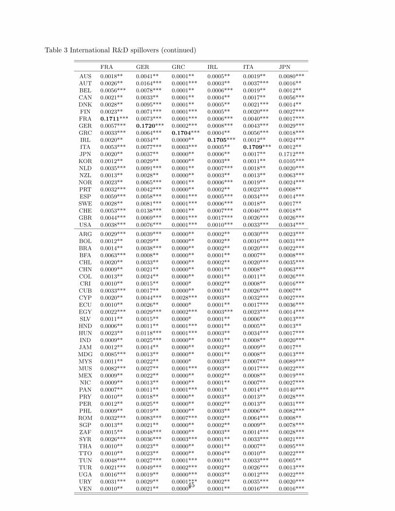
Table 3 International R&D spillovers (continued)

FRA GER GRC IRL ITA JPN

AUS 0.0018** 0.0041** 0.0001** 0.0005** 0.0019** 0.0080***AUT 0.0026** 0.0164*** 0.0001*** 0.0003** 0.0037*** 0.0016**BEL 0.0056*** 0.0078*** 0.0001** 0.0006*** 0.0019** 0.0012**CAN 0.0021** 0.0033** 0.0001** 0.0004** 0.0017** 0.0056***DNK 0.0028** 0.0095*** 0.0001** 0.0005** 0.0021*** 0.0014**FIN 0.0023** 0.0071*** 0.0001*** 0.0005** 0.0020*** 0.0027***FRA 0.1711*** 0.0073*** 0.0001*** 0.0006*** 0.0040*** 0.0017***GER 0.0057*** 0.1720*** 0.0002*** 0.0008*** 0.0043*** 0.0029***GRC 0.0033*** 0.0064*** 0.1704*** 0.0004** 0.0056*** 0.0018***IRL 0.0020** 0.0034** 0.0000** 0.1705*** 0.0012** 0.0024***ITA 0.0053*** 0.0077*** 0.0003*** 0.0005** 0.1709*** 0.0012**JPN 0.0020** 0.0037** 0.0000** 0.0006** 0.0017** 0.1712***KOR 0.0012** 0.0029** 0.0000** 0.0003** 0.0011** 0.0105***NLD 0.0035*** 0.0091*** 0.0001** 0.0007*** 0.0018** 0.0020***NZL 0.0013** 0.0028** 0.0000** 0.0003** 0.0013** 0.0063***NOR 0.0023** 0.0065*** 0.0001** 0.0006*** 0.0019** 0.0024***PRT 0.0032*** 0.0042*** 0.0000** 0.0002** 0.0023*** 0.0008**ESP 0.0059*** 0.0058*** 0.0001*** 0.0005*** 0.0034*** 0.0014***SWE 0.0028** 0.0081*** 0.0001*** 0.0006*** 0.0018** 0.0017**CHE 0.0053*** 0.0138*** 0.0001** 0.0007*** 0.0046*** 0.0018**GBR 0.0044*** 0.0069*** 0.0001*** 0.0017*** 0.0026*** 0.0026***USA 0.0038*** 0.0076*** 0.0001*** 0.0010*** 0.0033*** 0.0034***

ARG 0.0029*** 0.0039*** 0.0000** 0.0002** 0.0030*** 0.0023***BOL 0.0012** 0.0029** 0.0000** 0.0002** 0.0016*** 0.0031***BRA 0.0014** 0.0038*** 0.0000** 0.0002** 0.0020*** 0.0022***BFA 0.0063*** 0.0008** 0.0000** 0.0001** 0.0007** 0.0008***CHL 0.0020** 0.0033** 0.0000** 0.0002** 0.0020*** 0.0035***CHN 0.0009** 0.0021** 0.0000** 0.0001** 0.0008** 0.0063***COL 0.0013** 0.0024** 0.0000** 0.0001** 0.0011** 0.0026***CRI 0.0010** 0.0015** 0.0000* 0.0002** 0.0008** 0.0016***CUB 0.0033*** 0.0017** 0.0000** 0.0001** 0.0026*** 0.0007**CYP 0.0020** 0.0044*** 0.0028*** 0.0003** 0.0032*** 0.0027***ECU 0.0010** 0.0026** 0.0000* 0.0001** 0.0017*** 0.0036***EGY 0.0022*** 0.0029*** 0.0002*** 0.0003*** 0.0023*** 0.0014***SLV 0.0011** 0.0015** 0.0000* 0.0001** 0.0006** 0.0013***HND 0.0006** 0.0011** 0.0001*** 0.0001** 0.0005** 0.0013**HUN 0.0023** 0.0118*** 0.0001*** 0.0003** 0.0034*** 0.0017***IND 0.0009** 0.0025*** 0.0000** 0.0001** 0.0008** 0.0020***JAM 0.0012** 0.0014** 0.0000** 0.0002** 0.0009** 0.0017**MDG 0.0085*** 0.0013** 0.0000** 0.0001** 0.0008** 0.0013***MYS 0.0011** 0.0022** 0.0000* 0.0003** 0.0007** 0.0089***MUS 0.0082*** 0.0027** 0.0001*** 0.0003** 0.0017*** 0.0022***MEX 0.0009** 0.0022** 0.0000** 0.0002** 0.0008** 0.0019***NIC 0.0009** 0.0013** 0.0000** 0.0001** 0.0007** 0.0027***PAN 0.0007** 0.0011** 0.0001*** 0.0001* 0.0014*** 0.0140***PRY 0.0010** 0.0018** 0.0000** 0.0003** 0.0013** 0.0028***PER 0.0012** 0.0025** 0.0000** 0.0002** 0.0013** 0.0031***PHL 0.0009** 0.0019** 0.0000** 0.0003** 0.0006** 0.0082***ROM 0.0032*** 0.0083*** 0.0007*** 0.0002** 0.0064*** 0.0008**SGP 0.0013** 0.0021** 0.0000** 0.0002** 0.0009** 0.0078***ZAF 0.0015** 0.0048*** 0.0000** 0.0003** 0.0014*** 0.0028***SYR 0.0026*** 0.0036*** 0.0003*** 0.0001** 0.0033*** 0.0021***THA 0.0010** 0.0023** 0.0000** 0.0001** 0.0007** 0.0095***TTO 0.0010** 0.0023** 0.0000** 0.0004** 0.0010** 0.0022***TUN 0.0048*** 0.0027*** 0.0001*** 0.0001** 0.0033*** 0.0005**TUR 0.0021*** 0.0049*** 0.0002*** 0.0002** 0.0026*** 0.0013***UGA 0.0016*** 0.0019** 0.0000*** 0.0003** 0.0012*** 0.0022***URY 0.0031*** 0.0029** 0.0001*** 0.0002** 0.0035*** 0.0020***VEN 0.0010** 0.0021** 0.0000* 0.0001** 0.0016*** 0.0016***

45

Table 3 International R&D spillovers (continued)

KOR NLD NZL NOR PRT ESP

AUS 0.0020*** 0.0009** 0.0022*** 0.0002** 0.0001** 0.0005**AUT 0.0003** 0.0017** 0.0000** 0.0002** 0.0003** 0.0008**BEL 0.0003** 0.0062*** 0.0001** 0.0004** 0.0002** 0.0008**CAN 0.0017** 0.0007** 0.0002** 0.0011*** 0.0001** 0.0005**DNK 0.0004** 0.0032*** 0.0001** 0.0020*** 0.0005*** 0.0007**FIN 0.0005** 0.0019** 0.0000** 0.0017*** 0.0004*** 0.0007**FRA 0.0004** 0.0023*** 0.0000** 0.0007*** 0.0005*** 0.0024***GER 0.0006** 0.0045*** 0.0001** 0.0009*** 0.0005*** 0.0017***GRC 0.0008*** 0.0026*** 0.0001** 0.0002** 0.0002** 0.0012***IRL 0.0006** 0.0015** 0.0000** 0.0006*** 0.0002** 0.0006**ITA 0.0003** 0.0025*** 0.0001** 0.0003** 0.0002** 0.0016***JPN 0.0035*** 0.0007** 0.0005*** 0.0003** 0.0001** 0.0004**KOR 0.1708*** 0.0006** 0.0003*** 0.0002** 0.0000* 0.0003**NLD 0.0005** 0.1709*** 0.0000** 0.0009*** 0.0003*** 0.0010***NZL 0.0012** 0.0007** 0.1705*** 0.0002** 0.0001** 0.0003**NOR 0.0006** 0.0022*** 0.0000** 0.1706*** 0.0004*** 0.0008**PRT 0.0003** 0.0014*** 0.0000** 0.0004*** 0.1704*** 0.0050***ESP 0.0004** 0.0016*** 0.0000** 0.0003** 0.0009*** 0.1706***SWE 0.0004** 0.0029*** 0.0000** 0.0029*** 0.0004*** 0.0008**CHE 0.0004** 0.0025*** 0.0000** 0.0003** 0.0003** 0.0009**GBR 0.0007** 0.0033*** 0.0002*** 0.0012*** 0.0004*** 0.0013***USA 0.0040*** 0.0016** 0.0003*** 0.0006*** 0.0002** 0.0009**

ARG 0.0013*** 0.0008** 0.0001** 0.0001** 0.0001** 0.0019***BOL 0.0008** 0.0005** 0.0001** 0.0002** 0.0001** 0.0013***BRA 0.0009** 0.0007** 0.0001** 0.0002** 0.0001** 0.0007***BFA 0.0001** 0.0006** 0.0000* 0.0001** 0.0000** 0.0004***CHL 0.0018*** 0.0006** 0.0002*** 0.0002** 0.0001** 0.0015***CHN 0.0026*** 0.0004** 0.0001** 0.0001** 0.0000** 0.0002**COL 0.0008** 0.0005** 0.0000** 0.0001** 0.0000** 0.0008***CRI 0.0010** 0.0004** 0.0000** 0.0001** 0.0000** 0.0005***CUB 0.0001* 0.0010*** 0.0003*** 0.0001** 0.0001** 0.0070***CYP 0.0018*** 0.0010** 0.0001** 0.0005*** 0.0002** 0.0010***ECU 0.0010** 0.0006** 0.0001** 0.0001* 0.0001** 0.0012***EGY 0.0008*** 0.0007** 0.0001*** 0.0001** 0.0001** 0.0006***SLV 0.0008** 0.0003** 0.0002*** 0.0001* 0.0000** 0.0004**HND 0.0012** 0.0004** 0.0000** 0.0001* 0.0000* 0.0005***HUN 0.0005** 0.0016** 0.0000* 0.0002** 0.0002** 0.0007**IND 0.0008*** 0.0006** 0.0001** 0.0001** 0.0000** 0.0002**JAM 0.0008** 0.0007** 0.0002*** 0.0005*** 0.0000* 0.0010***MDG 0.0003*** 0.0004** 0.0000** 0.0001* 0.0001** 0.0004**MYS 0.0019*** 0.0005** 0.0002*** 0.0001** 0.0000** 0.0002**MUS 0.0007*** 0.0005** 0.0005*** 0.0001* 0.0001** 0.0005**MEX 0.0009** 0.0003** 0.0001** 0.0001* 0.0000* 0.0005**NIC 0.0013*** 0.0005** 0.0001** 0.0001** 0.0000** 0.0010***PAN 0.0045*** 0.0002* 0.0001** 0.0003*** 0.0000** 0.0004***PRY 0.0017*** 0.0004** 0.0000* 0.0001* 0.0001** 0.0005***PER 0.0015*** 0.0005** 0.0004*** 0.0001** 0.0000* 0.0012***PHL 0.0026*** 0.0006** 0.0003*** 0.0001* 0.0000* 0.0002**ROM 0.0011*** 0.0014** 0.0000** 0.0002** 0.0001** 0.0006**SGP 0.0017*** 0.0006** 0.0001** 0.0001** 0.0000** 0.0003**ZAF 0.0006** 0.0010** 0.0001** 0.0001** 0.0001** 0.0004**SYR 0.0016*** 0.0010** 0.0000** 0.0001** 0.0001** 0.0007***THA 0.0015*** 0.0005** 0.0002** 0.0001** 0.0000** 0.0002**TTO 0.0009** 0.0007** 0.0002*** 0.0001** 0.0001** 0.0004**TUN 0.0002** 0.0006** 0.0000** 0.0001** 0.0001** 0.0008***TUR 0.0006*** 0.0011** 0.0001** 0.0002** 0.0001** 0.0007***UGA 0.0004** 0.0007** 0.0000** 0.0003*** 0.0000** 0.0004***URY 0.0016*** 0.0007** 0.0001** 0.0001** 0.0001** 0.0025***VEN 0.0006** 0.0006** 0.0002*** 0.0001** 0.0001** 0.0007***

46

Table 3 International R&D spillovers (continued)

SWE CHE GBR USA

AUS 0.0010*** 0.0008** 0.0037*** 0.0121***AUT 0.0008** 0.0016*** 0.0017** 0.0025**BEL 0.0010*** 0.0007** 0.0035*** 0.0029**CAN 0.0007** 0.0006** 0.0033*** 0.0171***DNK 0.0047*** 0.0008** 0.0035*** 0.0026**FIN 0.0047*** 0.0009** 0.0037*** 0.0036***FRA 0.0007** 0.0011*** 0.0035*** 0.0038***GER 0.0012*** 0.0020*** 0.0038*** 0.0043***GRC 0.0007*** 0.0008** 0.0025*** 0.0019**IRL 0.0006** 0.0005** 0.0122*** 0.0062***ITA 0.0007** 0.0016*** 0.0026*** 0.0024**JPN 0.0007** 0.0010*** 0.0021** 0.0152***KOR 0.0004** 0.0007** 0.0014** 0.0112***NLD 0.0012*** 0.0008** 0.0042*** 0.0044***NZL 0.0008*** 0.0006** 0.0028*** 0.0086***NOR 0.0062*** 0.0007** 0.0043*** 0.0037**PRT 0.0004** 0.0005** 0.0019*** 0.0012**ESP 0.0006*** 0.0006** 0.0029*** 0.0027***SWE 0.1707*** 0.0009** 0.0042*** 0.0034***CHE 0.0009** 0.1707*** 0.0031*** 0.0037***GBR 0.0013*** 0.0014*** 0.1711*** 0.0059***USA 0.0012*** 0.0014*** 0.0052*** 0.1718***

ARG 0.0007*** 0.0007** 0.0015** 0.0101***BOL 0.0011*** 0.0005** 0.0011** 0.0109***BRA 0.0006*** 0.0007*** 0.0012** 0.0082***BFA 0.0001* 0.0001** 0.0006** 0.0009**CHL 0.0009*** 0.0006** 0.0014** 0.0115***CHN 0.0004** 0.0003** 0.0008** 0.0043***COL 0.0004** 0.0006*** 0.0011** 0.0103***CRI 0.0002** 0.0003** 0.0009** 0.0146***CUB 0.0003** 0.0003** 0.0010** 0.0008*CYP 0.0005** 0.0005** 0.0036*** 0.0022**ECU 0.0003** 0.0006** 0.0009** 0.0122***EGY 0.0005*** 0.0005** 0.0013** 0.0050***SLV 0.0002** 0.0003** 0.0007** 0.0116***HND 0.0002** 0.0004** 0.0007** 0.0146***HUN 0.0007*** 0.0011*** 0.0018** 0.0021**IND 0.0003** 0.0012*** 0.0020*** 0.0032***JAM 0.0003** 0.0004** 0.0017** 0.0168***MDG 0.0001** 0.0002** 0.0007** 0.0013**MYS 0.0004** 0.0006*** 0.0014** 0.0071***MUS 0.0002** 0.0008*** 0.0028*** 0.0012**MEX 0.0003** 0.0004** 0.0009** 0.0165***NIC 0.0002** 0.0002** 0.0007** 0.0105***PAN 0.0001* 0.0004** 0.0006** 0.0046**PRY 0.0003** 0.0004** 0.0017** 0.0116***PER 0.0006*** 0.0005** 0.0010** 0.0116***PHL 0.0003** 0.0004** 0.0010** 0.0083***ROM 0.0006** 0.0010*** 0.0019** 0.0025**SGP 0.0003** 0.0006*** 0.0015** 0.0073***ZAF 0.0004** 0.0008*** 0.0032*** 0.0041***SYR 0.0004*** 0.0004** 0.0012** 0.0021**THA 0.0004** 0.0006*** 0.0010** 0.0053***TTO 0.0003** 0.0003** 0.0036*** 0.0165***TUN 0.0003** 0.0003** 0.0006** 0.0011**TUR 0.0006*** 0.0007*** 0.0018*** 0.0029***UGA 0.0003** 0.0002** 0.0036*** 0.0017**URY 0.0004** 0.0008*** 0.0020*** 0.0070***VEN 0.0003** 0.0004** 0.0011** 0.0119***

Notes: *, ** and *** represent a level of significance of10%, 5% and 1% respectively.

47