A consistent compositional formulation for multiphase reactive transport where chemistry affects hydrodynamics

Advances in Water Resources 35 (2012) 83–93

Contents lists available at SciVerse ScienceDirect

Advances in Water Resources

journal homepage: www.elsevier .com/ locate/advwatres

A consistent compositional formulation for multiphase reactive transportwhere chemistry affects hydrodynamics

P. Gamazo a,b,⇑, M.W. Saaltink b, J. Carrera c, L. Slooten c, S. Bea d

a Water Department, North Headquarters, University of the Republic, Gral. Rivera 1350, 50000 Salto, Uruguayb GHS, Department Geotechnical Engineering and Geosciences, Universitat Politecnica de Catalunya, UPC-BarcelonaTech, c/Jordi Girona 1-3, 08034 Barcelona, Spainc GHS, Institute of Environmental Assessment and Water Research (IDAEA), CSIC, c/Lluis Solè Sabarìs, s/n, 08028 Barcelona, Spaind Earth Sciences Division, Lawrence Berkeley National Laboratory, One Cyclotron Road, M.S. 90-1116, Berkeley, CA 94720, USA

a r t i c l e i n f o a b s t r a c t

Article history:Received 29 April 2011Received in revised form 4 September 2011Accepted 6 September 2011Available online 13 October 2011

Keywords:Multiphase reactive transportCoupling effectsArid soil evaporationHydrated mineralsInvariant point

0309-1708/$ - see front matter � 2011 Elsevier Ltd. Adoi:10.1016/j.advwatres.2011.09.006

⇑ Corresponding author at: Water Department, Nortthe Republic, Gral. Rivera 1350, 50000 Salto, Uruguay

E-mail address: [email protected] (P. Gam

Multiphase reactive transport formulations usually decouple flow (i.e., phase conservation) from reactivetransport calculations (i.e., species conservation). Decoupling is not appropriate when reactions affectflow controlling variables (such as the partial pressure of gaseous components or the activity of water).We present a consistent compositional formulation that couples the conservation of all components. Noexplicit conservation of phases mass is required since they result from the conservation of all species ineach phase. The formulation acknowledges that constant activity species do not affect speciation and canbe eliminated, which reduces the number of unknowns. We discuss the formulation, the numerical solu-tion, and the implementation into an object oriented code. The advantages of the formulation are illus-trated by simulating the effect of mineral dehydration (including invariant points) on the hydrodynamicprocesses in an unsaturated column that reaches extremely dry conditions.

� 2011 Elsevier Ltd. All rights reserved.

1. Introduction

The most common approach for solving reactive transport prob-lems consists of decoupling the equations involved: first, the flowof fluid phases, and optionally energy transport; and, second, equa-tions for conservation of components, including chemical reac-tions. Single phase (saturated and unsaturated) reactive transportcodes uses this decoupled procedure [7,20,26,41]. The MIN3P code[24] couples gas flow and component conservation, but decouplesthe aqueous phase flow.

A similar approach is used by multiphase reactive transportcodes, such as TOUGHREACT [45], CODEBRIGHT-RETRASO [35],MUFTE-UG [11] and PFLOTRAN [21]. Instead of mass balancesof fluid phases, these codes adopt a compositional formulationthat establishes the mass balance of the dominant componentswithin each phase (e.g., water for the aqueous phase; dry airfor the gas phase; dry CO2 for the CO2 phase). Phase mass balanceresults from the mass balance of the major components. Theadvantage and motivation of these formulation lies in the elimi-nation of phase change terms, which is convenient since theseterms are usually associated to heterogeneous equilibrium reac-tions that lack explicit expressions. Phase pressures and fluxes,

ll rights reserved.

h Headquarters, University of.

azo).

and optionally temperature, are calculated in this first step. Theseare used as input for solving conservation equations of all chem-ical species.

This approach has been applied to a wide range of multiphasereactive transport problems. However it may be unsuitable whenfluxes and mass balances of major components depend on chemi-cal reactions. For example, when studying unsaturated tailings,oxygen is consumed by pyrite and Fe oxidation. It is clear thatthe effect of the oxygen consumption on gas flow cannot be eval-uated considering only dominant components (nitrogen and va-por) in the gaseous phase. A consistent approach, besidesincluding phase sink–source terms due to chemical reactions,should assure coherence between mass of the phase on one handand the species on the other. The mass of all species belonging toa phase should be equal to the mass of that phase. All this aspectsare difficult to represent by means of a decouple approach. Yet,none of the above codes consider them.

Soil salinization provides another example of dependency be-tween phase fluxes and chemical reactions. The amount of liquidwater in dry soils may be so small that both vapor and hydratedminerals become significant for the water balance. Wissmeierand Barry [43] addressed the effect of chemical sink–sources ofwater on liquid flow, for cases where transport is limited to unsat-urated liquid phase. This may not suffice for cases, such as soil sali-nization, when gas transport is important or when water activity,which controls vapor pressure, is affected by capillary and salinity.

Nomenclature

ai activity of species ia vector of the activities of all species a(i) = ai

aq sub index for the aqueous phaseci,a moles of the species i belonging to a phase a per phase

volumec vector of the concentration of all species c(i) = ci

caq vector of the concentration of aqueous speciescgas vector of the concentration of gaseous speciescimm,va vector of the concentration of immobile species with

variable activitycimm,ca vector of the concentration of immobile species with

constant activitydl, dt longitudinal and transversal dispersion coefficientsdf degrees of freedom of the systemdfph,rule Gibbs’s phase rule degrees of freedomdfph.dist degrees of freedom due to phase distributionDdiff

a diffusion coefficient of phase aDdisp

a dispersion coefficient for phases a Ddispa ¼ dtjqajIþ

ðdl � dtÞ qa �qtra

jqajfcap correction factor for water activity due to capillary ef-

fectsfi,a source sink term for species i belonging to a phase af vector of source–sink terms f(i) = fi

f0 external component source–sink term f = U � fg sub index for the gaseous phaseg gravity vectori sub index indicating a speciesj sub index indicating a reactionjDa ;i diffusive–dispersive flux of species i in phase a calcu-

lated by Fick’s law: jDa ;i ¼ Ddiffa /hasþDdisp

� �� rðci;aÞ

kra relative permeability for phase ak0 component source–sink term due to kinetic reactions

k0 = U � Sktr � rk

Kj equilibrium constant of reaction jK intrinsic permeabilityLa(ci,a) transport operator, null for immobile phases, for mobile

phases: Laðci;aÞ ¼ �r � ðci;aqaÞ �r � ðjDa ;iÞL() vector of transport operatorsmi molality of aqueous species ini moles of species iMi molecular weight of species iNc number of componentsNc0 number of reduced components Nc0 = Nc � Nca

Nca number of constant activity speciesNe number of equilibrium reactionsNk number of kinetic reactionsNs number of all speciesNsa number of species in phase aNxp number of primary speciesN0xp number of reduced primary speciesPi partial pressure of gaseous species iPa pressure of phase aqa flow of phase a, calculated by Darcy’s law:

qa ¼ � Kkralaðrpa � qagÞ

rej reaction rate of equilibrium reaction jre vector of equilibrium reaction rates re(j) = rej

rkj reaction rate of kinetic reaction jrk vector of kinetic reaction rates rk(j) = rkj

R Universal gas constantSej,i stoichiometric coefficient of equilibrium reaction j for

species iStr

e transpose of the equilibrium stoichiometric matrixStr

e (i,j) = Sej,i

Ski,j stoichiometric coefficient of kinetic reaction j for species iStr

k transpose of the kinetic stoichiometric matrixSk

tr(i, j) = Skj,i

Sa saturation of phase aT temperatureuaq vector of aqueous componentug vector of gaseous componentuimm,va vector of immobile components with variable activityU component matrixVg volume of the gaseous phasexi chemical concentration of species iZi compressibility factor of gaseous species ia sub index indicating a phaseci activity coefficient for aqueous species i,or fugacity

coefficient for gaseousha volumetric fraction of phase a ha = /Sala viscosity of phase aqa density of phase as tortuosity factor/ porosityvi

s molar fraction of mineral species i in the solid phasexi

a mass fraction of species i in phase a

84 P. Gamazo et al. / Advances in Water Resources 35 (2012) 83–93

In fact, extreme saline conditions may lead to precipitation ofhydrated minerals, which often produce invariant points. Theseare extreme cases in which chemical reactions generate sinks orsources that may be comparable to transport processes. Invariantpoints are defined as situations where mineral paragenesis(typically, simultaneous presence of several minerals with similarstoichiometry but different levels of hydration) prescribes theactivity of water [16,31]. One of the simplest examples of this isthe coexistence of gypsum and anhydrite. The activity of watercan be easily obtained by combining the mass action laws forgypsum and anhydrite equilibrium:

aCa2þaSO2�4

a2H2O ¼ Kgypsum

aCa2þaSO2�4¼ Kanhydrite ) aH2O ¼

ffiffiffiffiffiffiffiffiffiffiffiffiffiffiffiffiffiffiKgypsum

Kanhydrite

sð1Þ

where ai is the activity of the specie i and Kj is the equilibrium con-stant for reaction j.

In this case water activity value is kept fixed by a water sink–source term that results from combining gypsum and anhydriteformation reactions:

gypsum() anhydriteþ 2H2O ð2Þ

This sink–source affects not only the mass balance of the liquid, butalso that of the gas, since vapor partial pressure depends on wateractivity. Therefore, a fully coupled solution of phase fluxes and reac-tive transport is necessary. To the authors’ knowledge, due to thedifficulties they involve, invariant points have never been consid-ered in reactive transport problems.

Extending compositional formulation to all species in multi-phase reactive transport problems allows eliminating all equilib-rium reactions rates and not only the ones that affect majorcomponents. Compositional formulation also avoids consistencyproblems between phase balance and species balance, since no ex-plicit phase conservation equations are formulated. In fact,considering the mass balance of all species and phases leads to anon-independent system of equations.

P. Gamazo et al. / Advances in Water Resources 35 (2012) 83–93 85

Compositional formulations have been developed for a fixednumber of components [1,14,25,28], and for a general number[8,37,40] including linear sorption [2] and linear decay [29]. How-ever, compositional formulation do not include key processes forreactive transport, that are considered by codes that decouple flowfrom reactive transport, such as reactions between species of thesame phase (e.g., complexation and hydrolysis), biochemical pro-cesses, complex adsorption models or equilibrium with severalmineral phases (among others [6,22]). All these formulations de-fine components as the sum of species related to each otherthrough equilibrium heterogeneous reactions. However, a formula-tion is needed to account not only for heterogeneous reactions, butfor all types of reactions.

The aim of this paper is to present a general compositional for-mulation that can be used in cases where geochemical processessignificantly affect fluid flow, even when invariant points occur.For this, we first derive this formulation in Section 2. Then, in Sec-tion 3 we discuss its numerical solution. Section 4 contains anapplication that, despite of being conceptually simple, impliesstrong dependency between phase fluxes and chemical reactions.Finally, Section 5 is dedicated to summarize the conclusions.

2. Governing equation

Modeling multiphase reactive transport involves global and lo-cal equations. Global equations comprise partial differential equa-tions expressing conservation principles (mass, energy,momentum). Local equations include constitutive and thermody-namic expressions. Existing reactive transport formulations con-sider one set of equations to represent phase conservation (fromwhich flows are calculated) and another to represent componentsconservation. The fact that flow and reactive transport equationsare formulated and solved separately hinders the modeling of cou-pled effects. We present below a formulation which is based onlyon species conservation, and optionally energy conservation. Phaseconservation is simply the sum of the conservation of all speciesthat comprise that phase.

2.1. Global equation

The conservation of species i belonging to phase a can be ex-pressed as:

@

@thaci;a� �

¼ Laðci;aÞ þXNe

j¼1

Sej;i � rej þXNk

j¼1

Skj;i � rkj þ fi;a ð3Þ

where ha is volumetric content of the phase, ci,a is the concentrationof species i in phase a, Sej,i is the stoichiometric coefficient of speciesi for equilibrium reaction j and rej is the reaction rate of theequilibrium reaction j. Skj,i and rkj are analogous to Sej,i and rej butfor kinetic reactions. fi,a is a sink–source term, and La() is the trans-port operator of the mobile phase a that includes advection anddiffusion–dispersion Laðci;aÞ ¼ �r � ðci;aqaÞ �r � ðjDa ;iÞ. Mobilephase fluxes qa are calculated according to Darcy’s law anddiffusive–dispersive fluxes jDa ;i according to Fick’s law.

Note that Eq. (3) applies to all species, including liquid water.Thus, liquid water will be affected by advection and diffusion–dispersion. In what follows, conservation of all species in thesystem (Eq. (3)) is written using a vector–matrix notation:

@

@tðhcÞ ¼ LðcÞ þ Str

e � re þ Strk � rk þ f ð4Þ

where c is a vector containing the concentration of all speciesctr ¼ ctr

aq ctrgas ctr

imm;va ctrimm;ca

� �. We distinguish between aqueous,

caq , and gaseous species, cgas because the transport operator L() willbe different for each of them. Immobile species with variable activ-

ity, cimm,va, (like adsorbed species) are also distinguished fromimmobile constant activity species, cimm,ca, (normally minerals) be-cause, as shown by [33], the latter can be eliminated from compo-nent conservation equations. Str

e and Strk are the transpose of the

stoichiometric and kinetic matrices, respectively, re and rk are vec-tors containing the equilibrium and kinetic reaction rates and f is avector of external source–sink terms.

Equilibrium reaction rates (re) lack explicit expressions for theirevaluation. Their values are constrained by transport processes [9].Transport processes may drive the solution away from equilibriumbut equilibrium reactions will neutralize this effect. The lack of anexplicit expression for re is solved by re-formulating Eq. (4) interms of components, that are independent of equilibrium reac-tions [32]. This does not imply any loss of information or simplifi-cation, since all species can be represented as a combination of oneor more components [44]. Components can be defined through afully ranked kernel matrix U, termed component matrix, which isdefined so as to eliminate equilibrium reaction rates when Eq.(4) is multiplied by it.

U � Stre ¼ 0) U � Str

e � re ¼ 0 ð5Þ

Molins et al. [23] showed several ways of defining matrix U. We willconsider the component matrix introduced by Saaltink et al. [33] inwhich constant activity species are eliminated. Details on the calcu-lation of U are given in Appendix A. Its dimensions are [Nc0,Ns],where

Nc0 ¼ Ns� Ne� Nca ð6Þ

Ns is the number of all species, Ne is the number of equilibriumreactions and Nca is the number of constant activity species. Notethat the number of components Nc0 defined by matrix U is smallerthan the classic component number Nc = Ns � Ne [39].

By multiplying Eq. (4) by U we obtain:

@

@tðU � h � cÞ ¼ LðU � cÞ þ U � Str

k � rk þ U � f ð7Þ

By defining the aqueous, gaseous and immobile variable activityportions of the components

uaq¼U �

caq

000

0BBB@

1CCCA; ug¼U �

0cgas

00

0BBB@

1CCCA; uimm;va¼U �

00

cimm;va

0

0BBB@

1CCCA; ð8Þ

and their kinetic and external source–sink terms

k0 ¼ U � Strk � rk; f 0 ¼ U � f; ð9Þ

Eq. (7) can be written as:

@

@tðhaquaqÞ þ

@

@tðhgugÞ þ

@

@tðuimm;vaÞ ¼ LaqðuaqÞ þ LgðugÞ þ k0 þ f 0

ð10Þ

This is the conservation equation in terms of components. As men-tioned before, component matrix U eliminates constant activityspecies, therefore their concentration do not affect Eq. (10).

As dimensions of matrix U are [Nc0, Ns], the number of conser-vation equations is reduced from Ns to Nc0. Constant activity spe-cies may appear or disappear with time (e.g. due to completedissolution or appearance of new mineral species). Therefore, thenumber of components can change in time and space. This pro-duces spatial sub domains with different U definition, making Eq.(7) valid over each single sub domain and not over the entire do-main [32].

Temperature affects constitutive and thermodynamic relations.Therefore, the energy balance should be considered, whenever theproblem is not isothermal. This implies considering one extra par-

86 P. Gamazo et al. / Advances in Water Resources 35 (2012) 83–93

tial differential equation. Details about energy conservation equa-tion have been discussed by a number of authors [21,25,28]. Theenergy conservation equation considered in this formulation is de-tailed in Appendix B.

2.2. Local equations

2.2.1. Mobile phase properties and medium propertiesThe literature provides several models for density, viscosity and

diffusion coefficients of mobile phases [15]. All these parametersare expressed as an explicit function of pressure, temperatureand chemical composition of the phase.

Saturation of the porous medium is described by a retentioncurve. Several models (such as that of [42,5]) express saturationas an explicit function of capillary pressure and surface tension.These models also provide expressions for relative permeabilityof mobile phases.

2.2.2. Phase fluxesPhase fluxes are normally associated with phase conservation

equations. As in the proposed formulation no explicit phase con-servation is considered, phase fluxes are calculated according toDarcy’s law and treated as local equations.

2.2.3. Equilibrium reactionsSeveral processes can be expressed by equilibrium reaction:

complexation, and heterogeneous relations, such as adsorption,mineral precipitation–dissolution and dissolution of gasses. Atthermodynamic equilibrium they are all expressed by the mass ac-tion law, which relates the activities of the species (or fugacity forgases) involved in reactionj:

XNs

i¼1

Sej;i � log ai ¼ log Kj ð11Þ

where Sej,i is the stoichiometric coefficient for species i, ai is itsactivity (or fugacity) and Kj is the equilibrium constant of reactionj. Kj may depend on pressure and temperature. Equilibrium con-stants for adsorption reactions involving electrostatic models mayalso depend on surface potentials.

Activity, or fugacity for gases, represents the chemical availabil-ity of species. Given that these variables have a similar physicalmeaning, we will both term them activity and refer to them as a.Activity of species i can be written in a general way as:

ai ¼ cixi ð12Þ

The meaning of ci and xi depends on the phase to which the speciesbelongs. For aqueous species xi represents molality [mol/kgH2O]and ci the activity coefficient. Depending on the ionic strength,aqueous species activities can be considered equal to one or calcu-lated using models such as Debye–Hückel [10], or Pitzer [27].

The psychrometric law is used to calculate the capillary effecton water activity [12].

fcap ¼ expðpg � plÞ �MH2O

RTql

� �ð13Þ

where pg and pl are the gaseous and liquid pressure, MH2O is molarweight of water, R is the universal gas constant, T is temperatureand ql is liquid density. Thus, the water activity is:

aH2OðlÞ ¼ fcap � aosmoticH2OðlÞ

ð14Þ

where aosmoticH2OðlÞ

is the activity of liquid water given by the thermody-namic model considering only osmotic effects. For very dilute wateraosmotic

H2OðlÞequals one. For saline water it can be calculated from the

osmotic coefficient (u, [13]).

For gaseous species, xi represents partial pressure and ci

represents the fugacity coefficient. Depending on pressure andtemperature ci can be considered equal to one or calculated bymeans of models such as van der Waals or particular virial rela-tions [3].

Adsorbed species belong to interfaces between solid and fluidphases. Despite the fact that interfaces cannot be regarded as ther-modynamic phases, it is convenient to consider them as phases forreasons of simplicity. The activity of species belonging to interfacescannot be regarded as the product of two values (xi and ci), as forliquid or gaseous phases. However, in order to have a commonnotation for all phases, we will regard xi as the activity of the ad-sorbed species i and ci equal to one.

For mineral species, xi represents the solid molar fraction vis,

and ci represents an activity coefficient. When pure minerals areassumed, vi

s and ci equal one and, therefore, the mineral activityis equal to one.

2.2.4. Kinetic reactionsSeveral kinds of process can be represented by kinetic reactions:

mineral precipitation–dissolution, redox processes and microbio-logical degradations. There are several expressions for kinetic reac-tion rates, such as Monod or Lasaga [20]. For mineral precipitation/dissolution, a constitutive expression for surface area must beconsidered.

2.2.5. Phase concentrations and constraintsSpecies conservation (Eq. (3)) is formulated considering volu-

metric concentration ci,a, but geochemical models use differentconcentration units, xi, depending on the phase the species belongto. For each phase, there is a different relation between ci,a and xi.Moreover, each phase gives rise to an additional constraint that canbe inferred from the units of xi.

The concentration for species i belonging to the aqueous phase lis expressed as:

ci;l ¼ qlxH2Ol mi ð15Þ

where ql is aqueous density, xH2Ol is the mass fraction of water and

mi is molality of species i.Thermodynamic models for aqueous solutions use molality as

concentration unit (moles per solvent kilograms, in the case of li-quid water). Thus, the concentration of water, moles of water perwater kilograms, is constant. The mass fraction of water, xH2O

l ,can be calculated from the fact that by definition the sum of massfractions of all aqueous species equals 1:

1 ¼XNsaq

i

xil ¼

XNsaq

i

xH2Ol miMi ¼ xH2O

l 1þXNsaq

i–H2O

miMi

!

) xH2Ol ¼ 1þ

XNsaq

i–H2O

miMi

!�1

ð16Þ

where xil is the mass fraction of species i in the aqueous phase and

Mi its molar weight. Considering Eqs. (15) and (16) it can be seenthat the volumetric concentration of H2O can be expressed as afunction of the molities of all other aqueous species, and density.This expression will be used in Section 3.3, when defining the solu-tion variables.

The volumetric concentration of species i belonging to the gas-eous phase g can be obtained from the equation of state for the gas.Here we use the general gas law:

piVg ¼ niZiRT ) ni

Vg¼ pi

ZiRT

ci ¼pi

ZiRT

ð17Þ

P. Gamazo et al. / Advances in Water Resources 35 (2012) 83–93 87

where R is the universal gas constant, T is temperature, Vg is gas vol-ume, ni, pi and Zi are moles, partial pressure and compressibility fac-tor for gaseous species i, respectively. Zi values can be calculatedfrom virial relations or considered equal to one if the gas is assumedto be ideal.

Gas pressure can be expressed as a function of partial pressureof all gaseous species through Dalton’s law:

pg ¼XNsg

i¼1

pi ð18Þ

where pg is the gas pressure and Nsg is the number of gaseousspecies.

Mineral species must satisfy:

XNsm

i

vis ¼ 1 ð19Þ

where visolid is the molar fraction of mineral species i in mineral

phase s, and Nsm is the total number of mineral species in mineralphase m. Very often only pure minerals are considered. In that caseeach mineral phase is composed of only one mineral species andthus Eq. (19) becomes trivial.

3. Solution

3.1. Numerical approach

There are two generic approaches for solving reactive transportequations numerically: the Sequential Iteration Approach (SIA) andthe Direct Substitution Approach (DSA). The pros and cons of thesemethods have been discussed by a number of authors[30,44,39,34]. Both approaches require the sequential solution ofglobal and local equations.

We chose the DSA method because of it is robus and it is suit-able for the reduction of the number of components when constantactivity species are present. Chemical local equations produce aparticularly complex nonlinear system and its solution is knownas ‘‘speciation’’ in reactive transport argot. A methodology to solvespeciation is described in Section 3.3.

3.2. Degrees of freedom

All constitutive equations and thermodynamic models used inthe problem can be expressed as functions of temperature andpressures of the phases and their chemical composition as dis-cussed in Section 2.2. The minimum set of variables that allowsrepresenting phase composition and distribution constitutes thesolution variables of the problem. Gibbs’s phase rule indicatesthe number of thermodynamic degrees of freedom dfph,rule of asystem:

dfph;rule ¼ Nc � Nphþ 2 ð20Þ

where Nph is the number of phases. The phase rule gives the min-imum number of solution variables needed to calculate the chem-ical composition of all phases, but not the amount (or distribution)of the phases themselves. Hence, the system has additionaldegrees of freedom that correspond to the phase distribution[28]. As the sum of volume fractions of all phases should equalone, the number of degrees of freedom due to phase distributiondfph,dist is:

dfph;dist ¼ Nph� 1 ð21Þ

So, the total number of degrees of freedom of the system df is:

df ¼ dfph;rule þ dfph;dist ¼ Nc þ 1 ð22Þ

If the problem is isothermal the number of degrees of freedomwould be equal to the number of components. Saaltink et al. [33]have shown that constant activity species, can be eliminated fromthe system, reducing the number of components to Nc0. Thus, theminimal number of variables needed to represent phase composi-tion and distribution, and evaluate all constitutive relation is Nc0.This number is equal to the number of component conservationequations obtained in Section 2.1. Thus, all variables in the problemcan be calculated by solving component conservation equation (10).Given that constant activity species, such as minerals, might appearor disappear, the number of components Nc0 will change in time andspace. Concentration of constant activity species can be calculatedonce Eq. (10) has been solved.

3.3. Solutions variables and speciation

Speciation consists basically of calculating the chemical compo-sition of all phases (i.e., all species concentrations) from solutionvariables. The latter can be the concentrations of either compo-nents or primary species. Primary species are defined as a sub-group of species from which concentration of all other speciescan be calculated. We choose the concentration of the primary spe-cies as solution variables to facilitate speciation calculations, espe-cially when complex activity models are considered. It is easier tocalculate derivatives of activity coefficient with respect to primaryspecies than with respect to component concentration. Speciationis done by solving Eq. (11) for each of the Ne equilibrium reactions.Through these equations the concentration of the non-primaryspecies, termed secondary, are calculated as function of the con-centrations of the primary species. Note that the number of pri-mary species Nxp ¼ Ns� Nca� Ne ¼ Nc0 is equal to the number ofdegrees of freedom obtained in the previous section.

As mentioned earlier, the concentration of liquid water, molal-ity, is constant. Therefore, a different unknown is required. Appro-priate variables to characterize water could be the vapor pressure,the volumetric aqueous phase content, or liquid pressure, whichwe adopted here. Thus, the solution variables for speciation willbe the liquid pressure plus the chemical concentration of N0xp

pri-mary species N0xp

¼ Nxp � 1.

3.4. Solving the component conservation equations (discretization)

Several numerical techniques such as finite differences and finitevolumes are suitable for discretizing the partial differential equa-tions for component conservation(10). These techniques approxi-mate the solution at discrete entities of the domain (like cells ornodes) and generate a nonlinear set of ordinary equations. TheNewton–Raphson method is the most suitable for solving this non-linear set of equations. This method demands the evaluation andderivation of the discretized equations with respect to the solutionvariables, requiring the solution of all local equations (speciation).

Thus, two kinds of nonlinear systems have to be solved: a largeone for the global equations for component conservation and sev-eral small ones (one for each discrete entity) for the local equations(which includes speciation). Note that for each iteration of thelarge system it is necessary to solve all the small systems in orderto update secondary variables and their derivatives.

3.5. Calculation of constant activity species

Solution of component conservation yields the concentrationsof all species, except those of constant activity which had beeneliminated. Constant activity species concentrations can becalculated subsequently from the Ns species conservation equation(4). Once component conservation is solved, the only unknownsare the Nca constant activity species and the Ne equilibrium

88 P. Gamazo et al. / Advances in Water Resources 35 (2012) 83–93

reaction rates. The number of equations (Ns) is higher than thenumber of unknowns (Nca + Ne). Least square techniques couldbe used to solve these equations. An alternative is to remove someof the equations by only considering the secondary species. This re-sults in a system with the same number of unknowns andequations:

Ns� Nc0 ¼ Ns� ðNs� Ne� NcaÞ ¼ Neþ Nca ð23Þ

Note that this is exactly the same number of equations that wereeliminated when passing from species to component conservation(Eq. (6)).

4. Application: dynamics of multiphase flux and reactivetransport during evaporation from a gypsum column

4.1. Conceptual model

This formulation was implemented following the object ori-ented (OO) paradigm in a FORTRAN 95 code merging and expand-ing two existing OO codes PROOST [38] and CHEPROO [4]. PROOSTis a general purpose hydrological modeling tool that can solve alarge variety of conservation equations expressed as partial differ-ential equations. It was built and used to simulate flow and trans-port problems. CHEPROO is an OO tool specialized in complexgeochemical processes. While component mass balances are for-mulated in PROOST, all chemical aspects are handled by CHEPROO.For a given value of primary species, CHEPROO calculates the spe-ciation, checks whether the definition of components correspondsto the set of minerals, changing it if necessary, and calculates phaseproperties and component concentrations and their derivatives.PROOST uses these to solve the component mass balance equationby means of the finite element method applying the Newton–Raphson method for solving the resulting nonlinear system.

We applied this code to an evaporating soil column reaching ex-tremely dry conditions. Evaporation from soils involves liquid andgas fluxes, diffusion and energy transport. These phenomena inter-act with geochemistry especially in arid or semiarid environmentswith extreme dry conditions and high salt contents. In these envi-ronments water activity, which is a key parameter for evaporation,is influenced by osmotic effects because of high solute concentra-tions and by capillary effects because of low saturations. Theamount of liquid water can be so small that the water balancemay be significantly influenced by precipitation or dissolution ofhydrated minerals. A synthetic example was designed for illustrat-ing several features of the proposed formulation.

We modeled the evolution of a 24 cm column of porous gypsumsubject to a constant source of heat. The column was considered tobe initially saturated, at a temperature of 25 �C and open at itsupper part, permitting vapor exchange with the atmosphere dueto advection and diffusion. As extreme dry conditions are reached,we considered a retention curve capable of representing oven dryconditions. Although oven dry conditions are not reached, capillarypressure can reach values where conventional retention curvescannot be applied anymore [17,19,36]. The high ionic strengthnecessitates the use of the Pitzer ion interaction model (i.e.HWM model, [18]) to evaluate activities of aqueous species. Thecomplex ionic interactions affect dissolved ions activity and so,mineral solubility. Besides SO4, Ca and H2O, Cl and K were consid-ered. Problem parameters, constitutive models and boundary con-ditions are shown in Tables 1 and 2. We consider gypsum becauseit dehydrates forming anhydrite and acts as a chemical source ofwater that can affect flow. The species water (vapor) and air (amixture of 20% oxygen and 80% nitrogen) were considered forthe gaseous phase.

The column was discretized in 100 elements considering alength of 1 mm for the upper 80 elements, and a length of 8 mmfor the rest. An adaptive time step criteria was considered that var-ies the step size depending on the number of iteration of the solver.We considered an initial time step of 100 s and a maximum of 20iterations per time step.

4.2. Column evolution

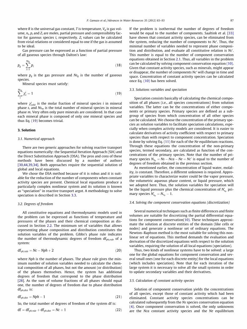
Saturation, vapor pressure, temperature and liquid flow profilesare shown in Fig. 1. The profile of the vapor pressure shows the for-mation of an evaporation front that moves downwards. This frontdivides the domain into two zones: a dry zone above the frontwhere extremely low saturations prevail and a humid zone below.The figure also shows a different temperature gradient for eachzone. The reason for this difference is that a large amount of energyis consumed at the evaporation front.

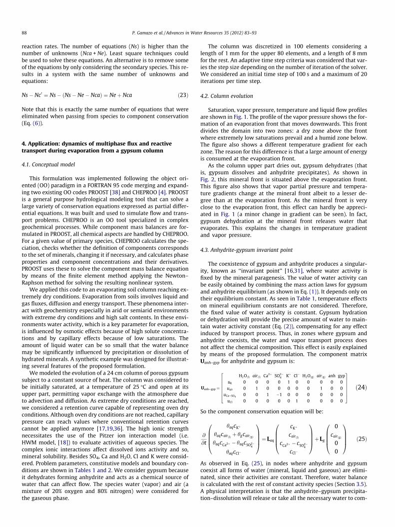
As the column upper part dries out, gypsum dehydrates (thatis, gypsum dissolves and anhydrite precipitates). As shown inFig. 2, this mineral front is situated above the evaporation front.This figure also shows that vapor partial pressure and tempera-ture gradients change at the mineral front albeit to a lesser de-gree than at the evaporation front. As the mineral front is veryclose to the evaporation front, this effect can hardly be appreci-ated in Fig. 1 (a minor change in gradient can be seen). In fact,gypsum dehydration at the mineral front releases water thatevaporates. This explains the changes in temperature gradientand vapor pressure.

4.3. Anhydrite-gypsum invariant point

The coexistence of gypsum and anhydrite produces a singular-ity, known as ‘‘invariant point’’ [16,31], where water activity isfixed by the mineral paragenesis. The value of water activity canbe easily obtained by combining the mass action laws for gypsumand anhydrite equilibrium (as shown in Eq. (1)). It depends only ontheir equilibrium constant. As seen in Table 1, temperature effectson mineral equilibrium constants are not considered. Therefore,the fixed value of water activity is constant. Gypsum hydrationor dehydration will provide the precise amount of water to main-tain water activity constant (Eq. (2)), compensating for any effectinduced by transport process. Thus, in zones where gypsum andanhydrite coexists, the water and vapor transport process doesnot affect the chemical composition. This effect is easily explainedby means of the proposed formulation. The component matrixUanh–gyp for anhydrite and gypsum is:

Uanh—gyp ¼

H2OðlÞ airðlÞ Ca2þ SO2�4 Kþ Cl� H2OðgÞ airðgÞ anh gyp

uK 0 0 0 0 1 0 0 0 0 0uair 0 1 0 0 0 0 0 1 0 0

uCa—SO4 0 0 1 �1 0 0 0 0 0 0uCl 0 0 0 0 0 1 0 0 0 0

26666664

37777775ð24Þ

So the component conservation equation will be:

@

@t

haqcKþ

haqcairðlÞ þ hgcairðgÞ

haqcCa2þ � haqcSO2�4

haqcCl�

0BBB@

1CCCA¼ Laq

cKþ

cairðlÞ

cCa2þ � cSO2�4

cCl�

0BBB@

1CCCAþLg

0cairðgÞ

00

0BBB@

1CCCA ð25Þ

As observed in Eq. (25), in nodes where anhydrite and gypsumcoexist all forms of water (mineral, liquid and gaseous) are elimi-nated, since their activities are constant. Therefore, water balanceis calculated with the rest of constant activity species (Section 3.5).A physical interpretation is that the anhydrite–gypsum precipita-tion–dissolution will release or take all the necessary water to com-

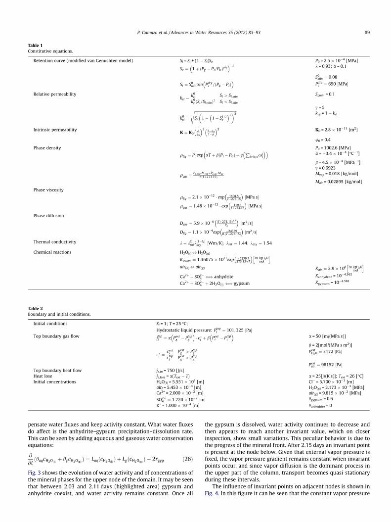
Table 1Constitutive equations.

Retention curve (modified van Genuchten model) Sl = Si + (1 � Si)Se P0 = 2.5 � 10�4 [MPa]

Se ¼ 1þ ðPg � Pl=P0Þ1

1�k

� ��k k = 0.93; a = 0.1

S0min ¼ 0:08

Si ¼ S0minaln Pdry

c =ðPg � PlÞ� �

Pdryc ¼ 650 ½MPa�

Relative permeabilitykrl ¼

k0rl Sl > Sl;min

k0rlðSl=Sl;minÞc Sl < Sl;min

Sl,min = 0.1

c = 5

k0rl ¼

ffiffiffiffiffiffiffiffiffiffiffiffiffiffiffiffiffiffiffiffiffiffiffiffiffiffiffiffiffiffiffiffiffiffiffiffiffiffiffiffiffiffiffiffiffiffiffiSe 1� 1� S1=k

e

� �k� �2

skrg = 1 � krl

Intrinsic permeabilityK ¼ K0

//0

� �3 1�/01�/

� �2 K0 = 2.8 � 10�11 [m2]

/0 = 0.4

Phase density P0 = 1002.6 [MPa]

qliq ¼ P0exp aT þ bðPl � P0Þ þ cP

i–h2 oxil

� �� �a = �3.4 � 10�4 [�C�1]

b = 4.5 � 10�4 [MPa�1]c = 0.6923

qgas ¼Pg;vap �MvapþPg;air �Mair

RðTþ273:15ÞMvap = 0.018 [kg/mol]

Mair = 0.02895 [kg/mol]

Phase viscosity

lliq ¼ 2:1� 10�12 � exp 1808:5Tþ273:15

� �½MPa s�

lgas ¼ 1:48� 10�12 � exp 119:4Tþ273:15

� �½MPa s�

Phase diffusion

Dgas ¼ 5:9� 10�6 ðTþ273:15Þ2:3Pg

� �½m2=s�

Dliq ¼ 1:1� 10�4exp �24539R�ðTþ273:15Þ

� �½m2=s�

Thermal conductivity k ¼ kSlsatk

ð1�SlÞdry ½Wm=K�; ksat ¼ 1:44; kdry ¼ 1:54

Chemical reactions H2O(l), H2O(g)

Kvapor ¼ 1:36075� 1011exp �5239:7273:15þT

� �Pa kgH2O

mol

h iair(k), air(g) Kair ¼ 2:9� 108 Pa kgH2 O

mol

h iCa2þ þ SO2�

4 () anhydrite Kanhydrite = 10�4.362

Ca2þ þ SO2�4 þ 2H2OðlÞ () gypsum Kgypsum = 10�4.581

Table 2Boundary and initial conditions.

Initial conditions Sl = 1; T = 25 �C;

Hydrostatic liquid pressure: Ptopl ¼ 101;325 ½Pa�

Top boundary gas flow jtopi ¼ a Pext

g � Ptopg

� �� c�i þ b Pext

i � Ptopi

� �a = 50 [m/(MPa s)]

b = 2[mol/(MPa s m2)]

c�i ¼cext

i Pextg > Ptop

g

ctopi Pext

g < Ptopg

PextH2O ¼ 3172 ½Pa�

Pextair ¼ 98152 ½Pa�

Top boundary heat flow je,in = 750 [J/s]Heat lose je,lose = a(Text � T) a = 25[J/(K s)]; Text = 26 [�C]Initial concentrations H2O(l) = 5.551 � 101 [m] Cl� = 5.700 � 10�3 [m]

airl = 5.453 � 10�4 [m] H2O(g) = 3.173 � 10�3 [MPa]Ca2+ = 2.000 � 10�2 [m] air(g) = 9.815 � 10�2 [MPa]

SO2þ4 ¼ 1:720� 10�2 ½m� hgypsum = 0.6

K+ = 1.000 � 10�4 [m] hanhydrite = 0

P. Gamazo et al. / Advances in Water Resources 35 (2012) 83–93 89

pensate water fluxes and keep activity constant. What water fluxesdo affect is the anhydrite–gypsum precipitation–dissolution rate.This can be seen by adding aqueous and gaseous water conservationequations:

@

@tðhaqcH2OðlÞ þ hgcH2OðgÞ Þ ¼ LaqðcH2OðlÞ Þ þ LgðcH2OðgÞ Þ � 2rgyp ð26Þ

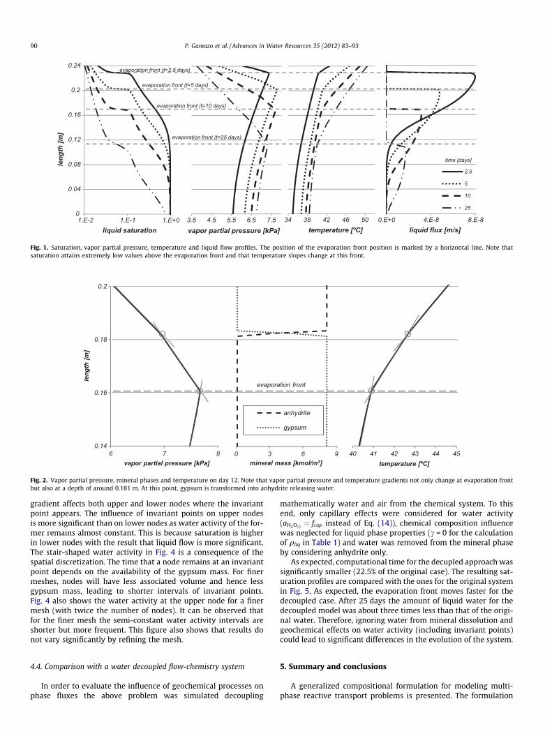
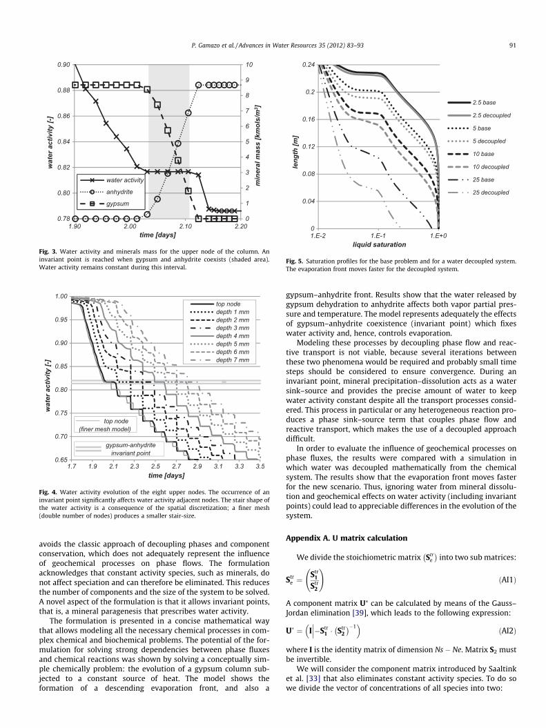
Fig. 3 shows the evolution of water activity and of concentrations ofthe mineral phases for the upper node of the domain. It may be seenthat between 2.03 and 2.11 days (highlighted area) gypsum andanhydrite coexist, and water activity remains constant. Once all

the gypsum is dissolved, water activity continues to decrease andthen appears to reach another invariant value, which on closerinspection, show small variations. This peculiar behavior is due tothe progress of the mineral front. After 2.15 days an invariant pointis present at the node below. Given that external vapor pressure isfixed, the vapor pressure gradient remains constant when invariantpoints occur, and since vapor diffusion is the dominant process inthe upper part of the column, transport becomes quasi stationaryduring these intervals.

The influence of invariant points on adjacent nodes is shown inFig. 4. In this figure it can be seen that the constant vapor pressure

0

0.04

0.08

0.12

0.16

0.2

0.24

1.E-2 1.E-1 1.E+0

leng

th [m

]

liquid saturation3.5 4.5 5.5 6.5 7.5vapor partial pressure [kPa]

34 38 42 46 50temperature [ºC]

0.E+0 4.E-8 8.E-8liquid flux [m/s]

2.5

5

10

25

time [days]

evaporation front (t=2.5 days)

evaporation front (t=5 days)

evaporation front (t=10 days)

evaporation front (t=25 days)

Fig. 1. Saturation, vapor partial pressure, temperature and liquid flow profiles. The position of the evaporation front position is marked by a horizontal line. Note thatsaturation attains extremely low values above the evaporation front and that temperature slopes change at this front.

evaporation front

0.14

0.16

0.18

0.2

6 7 8

leng

th [m

]

vapor partial pressure [kPa]0 3 6 9

mineral mass [kmol/m3]

anhydrite

gypsum

40 41 42 43 44 45temperature [ºC]

Fig. 2. Vapor partial pressure, mineral phases and temperature on day 12. Note that vapor partial pressure and temperature gradients not only change at evaporation frontbut also at a depth of around 0.181 m. At this point, gypsum is transformed into anhydrite releasing water.

90 P. Gamazo et al. / Advances in Water Resources 35 (2012) 83–93

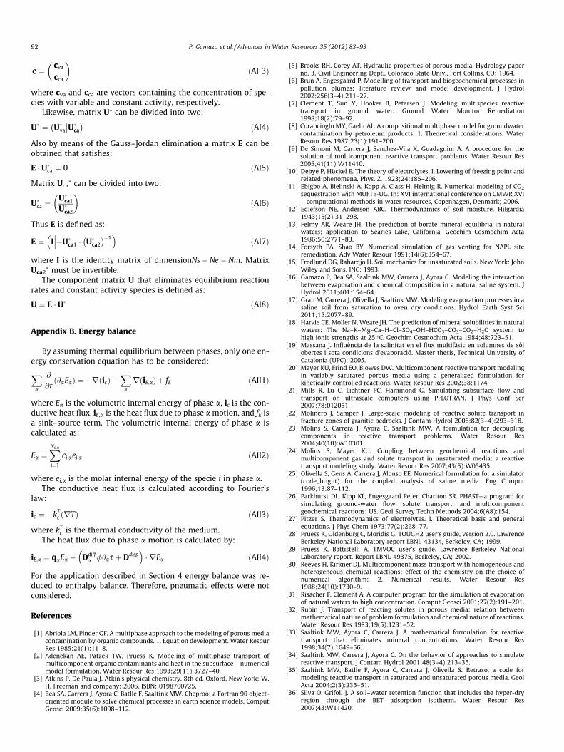
gradient affects both upper and lower nodes where the invariantpoint appears. The influence of invariant points on upper nodesis more significant than on lower nodes as water activity of the for-mer remains almost constant. This is because saturation is higherin lower nodes with the result that liquid flow is more significant.The stair-shaped water activity in Fig. 4 is a consequence of thespatial discretization. The time that a node remains at an invariantpoint depends on the availability of the gypsum mass. For finermeshes, nodes will have less associated volume and hence lessgypsum mass, leading to shorter intervals of invariant points.Fig. 4 also shows the water activity at the upper node for a finermesh (with twice the number of nodes). It can be observed thatfor the finer mesh the semi-constant water activity intervals areshorter but more frequent. This figure also shows that results donot vary significantly by refining the mesh.

4.4. Comparison with a water decoupled flow-chemistry system

In order to evaluate the influence of geochemical processes onphase fluxes the above problem was simulated decoupling

mathematically water and air from the chemical system. To thisend, only capillary effects were considered for water activity(aH2OðlÞ ¼ fcap instead of Eq. (14)), chemical composition influencewas neglected for liquid phase properties (c = 0 for the calculationof qliq in Table 1) and water was removed from the mineral phaseby considering anhydrite only.

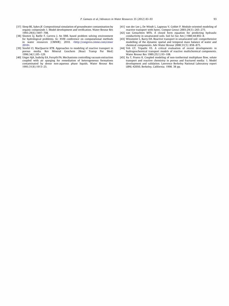
As expected, computational time for the decupled approach wassignificantly smaller (22.5% of the original case). The resulting sat-uration profiles are compared with the ones for the original systemin Fig. 5. As expected, the evaporation front moves faster for thedecoupled case. After 25 days the amount of liquid water for thedecoupled model was about three times less than that of the origi-nal water. Therefore, ignoring water from mineral dissolution andgeochemical effects on water activity (including invariant points)could lead to significant differences in the evolution of the system.

5. Summary and conclusions

A generalized compositional formulation for modeling multi-phase reactive transport problems is presented. The formulation

0

1

2

3

4

5

6

7

8

9

10

0.78

0.80

0.82

0.84

0.86

0.88

0.90

1.90 2.00 2.10 2.20

min

eral

mas

s [k

mol

s/m

3 ]

wat

er a

ctiv

ity [-

]

time [days]

water activity

anhydrite

gypsum

Fig. 3. Water activity and minerals mass for the upper node of the column. Aninvariant point is reached when gypsum and anhydrite coexists (shaded area).Water activity remains constant during this interval.

0.65

0.70

0.75

0.80

0.85

0.90

0.95

1.00

1.7 1.9 2.1 2.3 2.5 2.7 2.9 3.1 3.3 3.5

wat

er a

ctiv

ity [-

]

time [days]

top nodedepth 1 mmdepth 2 mmdepth 3 mmdepth 4 mmdepth 5 mmdepth 6 mmdepth 7 mm

gypsum-anhydriteinvariant point

top node(finer mesh model)

Fig. 4. Water activity evolution of the eight upper nodes. The occurrence of aninvariant point significantly affects water activity adjacent nodes. The stair shape ofthe water activity is a consequence of the spatial discretization; a finer mesh(double number of nodes) produces a smaller stair-size.

0

0.04

0.08

0.12

0.16

0.2

0.24

1.E-2 1.E-1 1.E+0

leng

th [m

]

liquid saturation

2.5 base

2.5 decoupled

5 base

5 decoupled

10 base

10 decoupled

25 base

25 decoupled

Fig. 5. Saturation profiles for the base problem and for a water decoupled system.The evaporation front moves faster for the decoupled system.

P. Gamazo et al. / Advances in Water Resources 35 (2012) 83–93 91

avoids the classic approach of decoupling phases and componentconservation, which does not adequately represent the influenceof geochemical processes on phase flows. The formulationacknowledges that constant activity species, such as minerals, donot affect speciation and can therefore be eliminated. This reducesthe number of components and the size of the system to be solved.A novel aspect of the formulation is that it allows invariant points,that is, a mineral paragenesis that prescribes water activity.

The formulation is presented in a concise mathematical waythat allows modeling all the necessary chemical processes in com-plex chemical and biochemical problems. The potential of the for-mulation for solving strong dependencies between phase fluxesand chemical reactions was shown by solving a conceptually sim-ple chemically problem: the evolution of a gypsum column sub-jected to a constant source of heat. The model shows theformation of a descending evaporation front, and also a

gypsum–anhydrite front. Results show that the water released bygypsum dehydration to anhydrite affects both vapor partial pres-sure and temperature. The model represents adequately the effectsof gypsum–anhydrite coexistence (invariant point) which fixeswater activity and, hence, controls evaporation.

Modeling these processes by decoupling phase flow and reac-tive transport is not viable, because several iterations betweenthese two phenomena would be required and probably small timesteps should be considered to ensure convergence. During aninvariant point, mineral precipitation–dissolution acts as a watersink–source and provides the precise amount of water to keepwater activity constant despite all the transport processes consid-ered. This process in particular or any heterogeneous reaction pro-duces a phase sink–source term that couples phase flow andreactive transport, which makes the use of a decoupled approachdifficult.

In order to evaluate the influence of geochemical processes onphase fluxes, the results were compared with a simulation inwhich water was decoupled mathematically from the chemicalsystem. The results show that the evaporation front moves fasterfor the new scenario. Thus, ignoring water from mineral dissolu-tion and geochemical effects on water activity (including invariantpoints) could lead to appreciable differences in the evolution of thesystem.

Appendix A. U matrix calculation

We divide the stoichiometric matrix Stre

� �into two sub matrices:

Stre ¼

Str1

Str2

!ðAI1Þ

A component matrix U⁄ can be calculated by means of the Gauss–Jordan elimination [39], which leads to the following expression:

U� ¼ I �Str1 � Str

2

� ��1� �

ðAI2Þ

where I is the identity matrix of dimension Ns � Ne. Matrix S2 mustbe invertible.

We will consider the component matrix introduced by Saaltinket al. [33] that also eliminates constant activity species. To do sowe divide the vector of concentrations of all species into two:

92 P. Gamazo et al. / Advances in Water Resources 35 (2012) 83–93

c ¼cva

cca

� �ðAI 3Þ

where cva and cca are vectors containing the concentration of spe-cies with variable and constant activity, respectively.

Likewise, matrix U⁄ can be divided into two:

U� ¼ U�va U�ca

� �ðAI4Þ

Also by means of the Gauss–Jordan elimination a matrix E can beobtained that satisfies:

E � U�ca ¼ 0 ðAI5Þ

Matrix Uca⁄ can be divided into two:

U�ca ¼U�ca1

U�ca2

� �ðAI6Þ

Thus E is defined as:

E ¼ I �U�ca1 � U�ca2

� ��1� �

ðAI7Þ

where I is the identity matrix of dimensionNs � Ne � Nm. MatrixUca2

⁄ must be invertible.The component matrix U that eliminates equilibrium reaction

rates and constant activity species is defined as:

U ¼ E � U� ðAI8Þ

Appendix B. Energy balance

By assuming thermal equilibrium between phases, only one en-ergy conservation equation has to be considered:X

a

@

@tðhaEaÞ ¼ �rðicÞ �

XarðiE;aÞ þ fE ðAII1Þ

where Ea is the volumetric internal energy of phase a, ic is the con-ductive heat flux, iE,a is the heat flux due to phase a motion, and fE isa sink–source term. The volumetric internal energy of phase a iscalculated as:

Ea ¼XNs;a

i¼1

ci;aei;a ðAII2Þ

where ei,a is the molar internal energy of the specie i in phase a.The conductive heat flux is calculated according to Fourier’s

law:

ic ¼ �kTc ðrTÞ ðAII3Þ

where kTc is the thermal conductivity of the medium.

The heat flux due to phase a motion is calculated by:

iE;a ¼ qaEa � Ddiffa /hasþ Ddisp

� �� rEa ðAII4Þ

For the application described in Section 4 energy balance was re-duced to enthalpy balance. Therefore, pneumatic effects were notconsidered.

References

[1] Abriola LM, Pinder GF. A multiphase approach to the modeling of porous mediacontamination by organic compounds. 1. Equation development. Water ResourRes 1985;21(1):11–8.

[2] Adenekan AE, Patzek TW, Pruess K. Modeling of multiphase transport ofmulticomponent organic contaminants and heat in the subsurface – numericalmodel formulation. Water Resour Res 1993;29(11):3727–40.

[3] Atkins P, De Paula J. Atkin’s physical chemistry. 8th ed. Oxford, New York: W.H. Freeman and company; 2006. ISBN: 0198700725.

[4] Bea SA, Carrera J, Ayora C, Batlle F, Saaltink MW. Cheproo: a Fortran 90 object-oriented module to solve chemical processes in earth science models. ComputGeosci 2009;35(6):1098–112.

[5] Brooks RH, Corey AT. Hydraulic properties of porous media. Hydrology paperno. 3. Civil Engineering Dept., Colorado State Univ., Fort Collins, CO; 1964.

[6] Brun A, Engesgaard P. Modelling of transport and biogeochemical processes inpollution plumes: literature review and model development. J Hydrol2002;256(3–4):211–27.

[7] Clement T, Sun Y, Hooker B, Petersen J. Modeling multispecies reactivetransport in ground water. Ground Water Monitor Remediation1998;18(2):79–92.

[8] Corapcioglu MY, Gaehr AL. A compositional multiphase model for groundwatercontamination by petroleum products. 1. Theoretical considerations. WaterResour Res 1987;23(1):191–200.

[9] De Simoni M, Carrera J, Sanchez-Vila X, Guadagnini A. A procedure for thesolution of multicomponent reactive transport problems. Water Resour Res2005;41(11):W11410.

[10] Debye P, Hückel E. The theory of electrolytes. I. Lowering of freezing point andrelated phenomena. Phys. Z. 1923;24:185–206.

[11] Ebigbo A, Bielinski A, Kopp A, Class H, Helmig R. Numerical modeling of CO2

sequestration with MUFTE-UG. In: XVI international conference on CMWR XVI– computational methods in water resources, Copenhagen, Denmark; 2006.

[12] Edlefson NE, Anderson ABC. Thermodynamics of soil moisture. Hilgardia1943;15(2):31–298.

[13] Felmy AR, Weare JH. The prediction of borate mineral equilibria in naturalwaters: application to Searles Lake, California. Geochim Cosmochim Acta1986;50:2771–83.

[14] Forsyth PA, Shao BY. Numerical simulation of gas venting for NAPL siteremediation. Adv Water Resour 1991;14(6):354–67.

[15] Fredlund DG, Rahardjo H. Soil mechanics for unsaturated soils. New York: JohnWiley and Sons, INC; 1993.

[16] Gamazo P, Bea SA, Saaltink MW, Carrera J, Ayora C. Modeling the interactionbetween evaporation and chemical composition in a natural saline system. JHydrol 2011;401:154–64.

[17] Gran M, Carrera J, Olivella J, Saaltink MW. Modeling evaporation processes in asaline soil from saturation to oven dry conditions. Hydrol Earth Syst Sci2011;15:2077–89.

[18] Harvie CE, Moller N, Weare JH. The prediction of mineral solubilities in naturalwaters: The Na–K–Mg–Ca–H–Cl–SO4–OH–HCO3–CO3–CO2–H2O system tohigh ionic strengths at 25 �C. Geochim Cosmochim Acta 1984;48:723–51.

[19] Massana J. Influència de la salinitat en el flux multifàsic en solumnes de sòlobertes i sota condicions d’evaporació. Master thesis, Technical University ofCatalonia (UPC); 2005.

[20] Mayer KU, Frind EO, Blowes DW. Multicomponent reactive transport modelingin variably saturated porous media using a generalized formulation forkinetically controlled reactions. Water Resour Res 2002;38:1174.

[21] Mills R, Lu C, Lichtner PC, Hammond G. Simulating subsurface flow andtransport on ultrascale computers using PFLOTRAN. J Phys Conf Ser2007;78:012051.

[22] Molinero J, Samper J. Large-scale modeling of reactive solute transport infracture zones of granitic bedrocks. J Contam Hydrol 2006;82(3–4):293–318.

[23] Molins S, Carrera J, Ayora C, Saaltink MW. A formulation for decouplingcomponents in reactive transport problems. Water Resour Res2004;40(10):W10301.

[24] Molins S, Mayer KU. Coupling between geochemical reactions andmulticomponent gas and solute transport in unsaturated media: a reactivetransport modeling study. Water Resour Res 2007;43(5):W05435.

[25] Olivella S, Gens A, Carrera J, Alonso EE. Numerical formulation for a simulator(code_bright) for the coupled analysis of saline media. Eng Comput1996;13:87–112.

[26] Parkhurst DL, Kipp KL, Engesgaard Peter, Charlton SR. PHAST—a program forsimulating ground-water flow, solute transport, and multicomponentgeochemical reactions: US. Geol Survey Techn Methods 2004;6(A8):154.

[27] Pitzer S. Thermodynamics of electrolytes. I. Theoretical basis and generalequations. J Phys Chem 1973;77(2):268–77.

[28] Pruess K, Oldenburg C, Moridis G. TOUGH2 user’s guide, version 2.0. LawrenceBerkeley National Laboratory report LBNL-43134, Berkeley, CA; 1999.

[29] Pruess K, Battistelli A. TMVOC user’s guide. Lawrence Berkeley NationalLaboratory report. Report LBNL-49375, Berkeley, CA; 2002.

[30] Reeves H, Kirkner DJ. Multicomponent mass transport with homogeneous andheterogeneous chemical reactions: effect of the chemistry on the choice ofnumerical algorithm: 2. Numerical results. Water Resour Res1988;24(10):1730–9.

[31] Risacher F, Clement A. A computer program for the simulation of evaporationof natural waters to high concentration. Comput Geosci 2001;27(2):191–201.

[32] Rubin J. Transport of reacting solutes in porous media: relation betweenmathematical nature of problem formulation and chemical nature of reactions.Water Resour Res 1983;19(5):1231–52.

[33] Saaltink MW, Ayora C, Carrera J. A mathematical formulation for reactivetransport that eliminates mineral concentrations. Water Resour Res1998;34(7):1649–56.

[34] Saaltink MW, Carrera J, Ayora C. On the behavior of approaches to simulatereactive transport. J Contam Hydrol 2001;48(3–4):213–35.

[35] Saaltink MW, Batlle F, Ayora C, Carrera J, Olivella S. Retraso, a code formodeling reactive transport in saturated and unsaturated porous media. GeolActa 2004;2(3):235–51.

[36] Silva O, Grifoll J. A soil–water retention function that includes the hyper-dryregion through the BET adsorption isotherm. Water Resour Res2007;43:W11420.

P. Gamazo et al. / Advances in Water Resources 35 (2012) 83–93 93

[37] Sleep BE, Sykes JF. Compositional simulation of groundwater contamination byorganic compounds 1. Model development and verification. Water Resour Res1993;29(6):1697–708.

[38] Slooten LJ, Batlle F, Carrera J. An XML based problem solving environmentfor hydrological problems. In: XVIII conference on computational methodsin water resources (CMWR); 2010. <http://congress.cimne.com/cmwr2010>.

[39] Steefel CI, MacQuarrie KTB. Approaches to modeling of reactive transport inporous media. Rev Mineral Geochem (React Transp Por Med)1996;34(1):85–129.

[40] Unger AJA, Sudicky EA, Forsyth PA. Mechanisms controlling vacuum extractioncoupled with air sparging for remediation of heterogeneous formationscontaminated by dense non-aqueous phase liquids. Water Resour Res1995;31(8):1913–25.

[41] van der Lee j, De Windt L, Lagneau V, Goblet P. Module-oriented modeling ofreactive transport with hytec. Comput Geosci 2003;29(3)::265–275.

[42] van Genuchten MTh. A closed form equation for predicting hydraulicconductivity in unsaturated soils. Soil Sci Soc Am J 1980;44:892–8.

[43] Wissmeier L, Barry DA. Reactive transport in unsaturated soil: comprehensivemodelling of the dynamic spatial and temporal mass balance of water andchemical components. Adv Water Resour 2008;31(5)::858–875.

[44] Yeh GT, Tripathi VS. A critical evaluation of recent developments inhydrogeochemical transport models of reactive multichemical components.Water Resour Res 1989;25(1):93–108.

[45] Xu T, Pruess K. Coupled modeling of non-isothermal multiphase flow, solutetransport and reactive chemistry in porous and fractured media: 1. Modeldevelopment and validation. Lawrence Berkeley National Laboratory reportLBNL-42050, Berkeley, California; 1998. 38 pp.