A Confidence Interval for Default and Prepayment Predictions of Manufactured Housing Seasoned Loans 1 (Draft, December 2006) Frederic N Wandey ♣ Department of Applied Economics University of Minnesota Abstract Competing risk hazard functions are estimated to predict prepayment and default probabilities for Manufactured Housing (MH) seasoned loans using proprietary loan- level data composed of MH loans booked between January 1996 and September 2004. Results show that variables used to capture option price theory in the literature on mortgage termination affect MH borrowers differently. Land-home borrowers are more likely to behave in a way consistent with the predictions of the theory, while chattel borrowers are more likely to put their mortgage even when it is in the money not to do so. Then, the study uses bootstrapping to estimate a confidence interval to the predicted conditional default (CDR) and prepayment rates (CPR). Validations’ results not only confirm stability of the parameter estimates but also show that actual CDR and CPR lie within the estimated confidence intervals. 1 This paper is an extract of my dissertation on Manufactured Housing Seasoned Loans: Default and Prepayment Predictions, and Racial Discrimination. I thank Samuel Myers, Paul Glewwe, Glen Pederson and Elisabeth Davis for their valuable comments during the conception of this project. I am also grateful for comments from participants at the Applied Economics Workshop at the University of Minnesota. All remaining errors are those of the author. ♣ Department of Applied Economics, University of Minnesota, 1994 Buford Avenue, Suite 218, St. Paul, MN 55414, USA. E-mail: [email protected]

Welcome message from author
This document is posted to help you gain knowledge. Please leave a comment to let me know what you think about it! Share it to your friends and learn new things together.
Transcript
A Confidence Interval for Default and Prepayment Predictions of Manufactured Housing Seasoned Loans1
(Draft, December 2006)
Frederic N Wandey♣ Department of Applied Economics
University of Minnesota
Abstract
Competing risk hazard functions are estimated to predict prepayment and default probabilities for Manufactured Housing (MH) seasoned loans using proprietary loan-level data composed of MH loans booked between January 1996 and September 2004. Results show that variables used to capture option price theory in the literature on mortgage termination affect MH borrowers differently. Land-home borrowers are more likely to behave in a way consistent with the predictions of the theory, while chattel borrowers are more likely to put their mortgage even when it is in the money not to do so. Then, the study uses bootstrapping to estimate a confidence interval to the predicted conditional default (CDR) and prepayment rates (CPR). Validations’ results not only confirm stability of the parameter estimates but also show that actual CDR and CPR lie within the estimated confidence intervals.
1 This paper is an extract of my dissertation on Manufactured Housing Seasoned Loans: Default and Prepayment Predictions, and Racial Discrimination. I thank Samuel Myers, Paul Glewwe, Glen Pederson and Elisabeth Davis for their valuable comments during the conception of this project. I am also grateful for comments from participants at the Applied Economics Workshop at the University of Minnesota. All remaining errors are those of the author. ♣ Department of Applied Economics, University of Minnesota, 1994 Buford Avenue, Suite 218, St. Paul, MN 55414, USA. E-mail: [email protected]
© Frederic N Wandey, December 2006.
2
The growth of mortgage and asset-backed securities in the 1990s has given rise to
a body of literature on mortgage defaults and prepayments focused on either commercial
mortgage or conventional residential mortgage markets2. This paper addresses two
challenges left in the dark of this literature. First, it focuses on manufactured housing
(MH) loans’ default and prepayment probabilities. Second, it estimates a confidence
interval to minimize the hedge taken by investors financing these types of loans. The
accuracy of the forecasted conditional default and prepayment rates are crucial given that
they are used as key assumptions in financial processes used to value and determine
underwriting standards for loan originations, portfolio acquisitions, and pool
securitizations.
Even though manufactured housing loans are similar to residential mortgages by
their characteristics, they differ from them in the following ways. First, the collateral
often depreciates over time, not only making it harder to apply option price theory to
prepayment/refinance behavior, but also creating incentives to default. Moreover, the
economic variables susceptible to capture consumer behavior seem not to have the same
impact on the loan termination than on the conventional mortgage, raising the need for a
confidence interval for an efficient implementation of the estimated parameters.
This work is divided into 5 sections. The first contains a brief introduction to MH.
Section 2 reviews the literature on mortgage prepayment and default models and sets up
the theoretical and empirical models. Section 3 provides a description of the data. Section
4 discusses the parameter estimates and validation of the models. Section 5 provides a
confidence interval for the models.
2 Recent studies were consecrated to subprime mortgage markets given the increase of subprime lending in the last ten years (Gjaja and al., 2004 & 2005; Danis and Pennington-Cross, 2005a; Danis and Pennington-Cross, 2005b).
© Frederic N Wandey, December 2006.
3
1. Manufactured Housing: Definition and Facts Manufactured housing is a term used to define housing units that are assembled in
factories and then transported to their sites of use. Even though the term’s general use
includes both mobile homes and modular homes, its technical use is restricted to mobile
homes, i.e. a class of homes regulated by the Federal National Manufactured Housing
Construction and Safety Standards Act of 1974. This Act directed the Department of
Housing and Urban Development to create a national building code that would make
mobile homes safer by reducing their vulnerability to high winds and fire (Hart et al.,
2002). The 1980 Housing Act changed the official legal name of mobile homes to
manufactured housing. The technical difference between modular and mobile homes is
that modular homes are usually hauled to their use locations on flat-bed trucks rather than
being towed, and they lack the axles and an automotive-type frame typical of mobile
homes. Both are properly referred to as manufactured housing.
The type of manufactured housing this paper will be focusing on is mobile homes.
They are defined as movable dwellings, 8 feet or more wide and 40 feet or more long,
designed to be towed on their own chassis, with transportation gear integral to the units
when they leave the factory. They are housing units built in factories, rather than on site,
and are taken to the place where they will be occupied, usually carried by tractor-trailers
over public highways. They are built in a controlled factory environment on a permanent
chassis to be used with or without a permanent foundation when connected to the
required utilities.
The two major types of mobile homes are “single-wide” and “double-wide.”
"Single-wide" are sixteen feet or less in width and are towed to their site as a single unit,

© Frederic N Wandey, December 2006.
4
whereas "double-wide" are twenty-four feet or more wide and are towed to their site in
two separate units, which are then joined together.
Mobile homes are usually much less expensive than site-built homes, and are
often associated with rural areas and high-density developments sometimes referred to as
trailer parks. For many low and moderate-income families, adequate site-built housing is
out of reach. Because of their lower cost manufactured housing is traditionally, although
certainly not always, used by lower-income people. Moreover, the fact that they are
perceived to depreciate in value much more quickly than site-built homes has led to
prejudice and negative zoning restrictions, built around the stereotypical concept of a
trailer park. Early mobile homes, even well-maintained ones, tended to depreciate in
value over time like motor vehicles rather than appreciate in value, as is typically the case
with site-built homes. The arrival of mobile homes in an area tended to be regarded with
alarm, particularly by the owners of more valuable real estate who often feared that their
property values would become depressed (See Munneke and Carlos Slawson, 1999).
This combination of factors led most jurisdictions to enact restrictive zoning
regulations concerning the areas in which mobile homes can be placed, as well as the
number and density of mobile homes permissible on any given site. Often other
restrictions, particularly minimum size requirements, limitations on exterior colors and
finishes, and mandatory specifications regarding foundations were enacted as well. Many
jurisdictions will not allow any additional mobile homes, and others have strongly limited
or forbidden entirely all single-wide models, which tend to depreciate more rapidly in
value than modern double-wide models.
© Frederic N Wandey, December 2006.
5
Despite the stigma associated with life in mobile homes, studies have shown that
there are nevertheless many reasons people live in mobile homes (Wallis, 1991; Hart et
al., 2002). These studies also show that mobile home owners are not necessarily low-
income people with challenged credit, limited skills and limited education. The category
of people who buy mobile homes has been widening over time.
Wallis (1991) shows that two processes have shaped the use, form, and meaning
of mobile homes. The first process is one of invention, or innovation, carried out by
mobile home manufacturers, park developers, and the people who live in mobile homes.
These people, driven by necessity and entrepreneurship, have created a new form of
housing, figured out how to relate it to land and community, how to finance, insure, and
otherwise protect and market it (Wallis, 1991). Mobile home manufacturers have
improved standards of construction over time and present their products as alternatives to
conventional site-built homes. According to Hart et al. (2002), one of every five new
single-family housing units purchased in the United States is a mobile home, sited
anywhere from the conventional trailer park to custom-designed “estates” aimed at young
couples and retirees.
The second process affecting the mobile home sector has been one of regulation
or categorization carried out primarily by institutions: zoning and building agencies,
mortgage bankers, and insurance companies. These two processes together – one pushing
at the boundaries of affordability and the other increasing standards of acceptability -
have given rise to a differentiated market of manufactured housing. The quality and
features of new MH models leads to greater acceptance by a growing segment of the
marketplace. Additionally, insurers and lenders are now more likely to treat the higher-
© Frederic N Wandey, December 2006.
6
end double-wide as they would a traditional home with regard to coverage and lending
practices (Jewell, 2003). Notwithstanding there is still a market for the traditional mobile
home, as the demand for housing continues to grow and the price of site-built housing
will more likely continue to increase.
Two factors are determinant in the segmentation of MH products in this study: the
site and the width of the home. Based on the site where the home will be placed, there are
two types of MH loans. One type funds both the home and the land on which the home is
placed. This type of loan will be designated as a land-home (LH) loan. A financial
institution could as well finance only a mobile home, which will be placed either on a
rented spot in a trailer park (park loans) or on privately owned land (non park loans). This
second type of product is known as chattels (CH). LH loans are usually a larger amount
than chattels, and LH collateral tends to hold value better than chattels. Also, the
empirical hazards graphed in section 3 show that LH loans tend to perform better than
chattels in the sense that will be made explicit in the empirical part of the paper. The
width of mobile homes is the second factor explaining loan amounts and performances.
Double-wide homes are more expensive than single-wide ones. They tend to hold value
better and outperform single-wide homes in terms of default and prepayment rates.
2. Determinant of Mortgage Termination This paper builds on three kinds of models in the literature on mortgage
termination. The first are the econometric valuation models, which rely heavily on data
mining techniques involving statistical analysis of historical prepayment and default data.
The major characteristic of this trend is that statistical significance determines the
© Frederic N Wandey, December 2006.
7
retention criteria of factors driving mortgage termination and, therefore, behavioral
theory plays a minor role when selecting predictors of mortgage termination.
This trend characterizes the first generation of mortgage termination models
developed in the mortgage industry where the availability of data permitted statistical
inference to be used to mine business decisions. The modeling techniques used in this
first generation of mortgage termination models are a transfer of consumer score card
techniques commonly used for revolving accounts. The focus on credit risk obliterate the
importance of simultaneously modeling market risk which became a big component of
mortgage cash flow management, particularly in the interest rate and house price
environments of the 1990’s. The emphasis on data mining constitutes the main drawback
for this type of modeling work as their results are vulnerable to changes in economic
factors affecting borrowers’ choices to prepay or default. This paper departs from this
trend by relying on behavioral theory and doing more than a simple stepwise estimation
of default and prepayment.
The second approach is the option-theoretic approach (Black and Scholes, 1973;
Merton, 1973; Dunn and McConnell, 1981; Deng, 1997). Option theory has been the
dominant paradigm for research on residential mortgage prepayment and default. An
option is a contract, or a provision of a contract, that gives the holder the right, but not the
obligation, to buy (or, alternatively, to sell) a set quantity of a particular asset at a set
price on, or up to, a given future date. If the contract is an option to buy, it is a “call”
option; if it is an option to sell, it is a “put” option. Similarly, a mortgage is considered as
a contract that gives the homeowner the right to call, i.e. buy the mortgage back from the
lender, or to put, i.e. sell (give up) to the lender the property right on the asset backing the
© Frederic N Wandey, December 2006.
8
contract. A mortgage can be seen as an “American option,” as opposed to a “European
option,” given that it can be exercised at any time up to the date the option expires (Black
and Scholes, 1973). The decision to exercise a call or put option is driven by the extent to
which the embedded options to prepay or default are “in the money.” The theory holds
that mortgage borrowers will exercise embedded call (prepayment) or put (default)
options when either of these options are “in the money” (Deng et al., 2000; and Calhoun
and Deng, 2002).
The assumption driving the option-theoretic approach to mortgages is that even
though mortgages depend on the real economy through the process describing changes in
the term structure and the house price, the valuation of mortgages does not necessarily
depend on the variables determining the underlying economy (Kau and Keenan, 1995).
These variables can be considered as exogenously determined by the prevailing state of
the nature and then factored into the borrower’s valuation of the mortgage. A mortgage’s
valuation is entirely explained by arbitrage reasoning as put forth by Arrow-Debreu’s
(AD) seminal work on assets valuations in markets with uncertainty (1954). Indeed, the
key idea behind the theoretical approach to mortgage termination is the no arbitrage
opportunity condition; i.e. the absence of a position in the marketplace with a positive
probability of realizing a profit without taking a risk. This idea constitutes the building
block of the results in the contingent claims models by Black and Scholes (1973)
hereafter BS, Merton (1973), and Cox, Ingersoll, and Ross (1985).
BS is indeed the basis of the literature on mortgage termination. According to BS,
the current value of the option is approximately equal to the price of the underlying asset
minus the price of a pure discount bond that matures at the same date as the option, with
© Frederic N Wandey, December 2006.
9
a face value equal to the striking price of the option. Formally, a call option with strike
price K at maturity date t+H is a function of the current price of the underlying asset St
and of the short-term interest rt:
);,,,(),( σHKrSpHKP ttBSt =
where σ is the volatility parameter. Given observed asset prices St, interest rates rt, and
derivative price Pt(Kj, H), the no arbitrage condition and the completeness of markets
imply that BS volatility, defined as the solution of
))(;,,,(),( KjHKjrSpHKP ttBSjt σ=
is an infinitely accurate estimator of ∧
σ . Such a conclusion is the shortcoming of the BS
model, as different strike prices Kj can lead to different estimates of ∧
σ (See Clement et
al., 2000).
On one hand, the present study expands upon the contingent claims models, as
these models emphasize the fact that the value of the mortgage is correlated with
underlying state variables (interest rate and house price) whose values are derived from
the process determining the economic environment3. The apparent difficulty of linking
3 As shown in the summary by Kau and Keenan (1995), the values of the term structure and the house price are derived from the process describing the true economic environment relevant to the mortgage as follows: rrr dztHrdttHrdr ),,(),,( σμ += (1)
HHH dztHrdttHrdH ),,(),,( σμ += (2) with
dttHrdzdz Hr ),,(, σ= (3)
where H is the house price, r the spot rate, rdz and Hdz are standard Wiener process with [ ] 0=dzE
and [ ] dtdzE =2 , and σ capturing the correlation between the disturbances to the house price and those of the term structure. The Wiener process term z assures that the actual changes in the interest rate and house price differ from the expected changes in an unbiased way because of normally distributed, serially uncorrelated disturbances to the economy.
© Frederic N Wandey, December 2006.
10
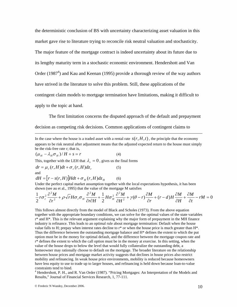
the deterministic conclusion of BS with uncertainty characterizing asset valuation in this
market gave rise to literature trying to reconcile risk neutral valuation and stochasticity.
The major feature of the mortgage contract is indeed uncertainty about its future due to
its lengthy maturity term in a stochastic economic environment. Hendershott and Van
Order (19874) and Kau and Keenan (1995) provide a thorough review of the way authors
have strived in the literature to solve this problem. Still, these applications of the
contingent claim models to mortgage termination have limitations, making it difficult to
apply to the topic at hand.
The first limitation concerns the disputed approach of the default and prepayment
decision as competing risk decisions. Common applications of contingent claims to In the case where the house is a traded asset with a rental rate ),,( tHrs , the principle that the economy appears to be risk neutral after adjustment means that the adjusted expected return to the house must simply be the risk-free rate r; that is,
rsHHHH =+− /)( σλμ (4)
This, together with the LEH that 0=rλ , gives us the final forms
rrr dzHrdtHrdr ),(),( σμ += (5) and
[ ] HH dzHrHdtHrsrdH ),(),( σ+−= (6) Under the perfect capital market assumption together with the local expectations hypothesis, it has been shown (see au et al., 1995) that the value of the mortgage M satisfies
0)()(21
21
2
22
2
2
22 =−
∂∂
+∂∂
−+∂∂
−+∂∂
+∂∂
∂+
∂∂ rM
tM
HMHdr
rMr
HMH
HrMHr
rMr HHrr θγσσσρσ
This follows almost directly from the model of Black and Scholes (1973). From the above equation together with the appropriate boundary conditions, we can solve for the optimal values of the state variables r* and H*. This is the relevant argument explaining why the major form of prepayment in the MH finance industry is refinance. This leads to an optimal rule about mortgage termination: Default when the house value falls to H; prepay when interest rates decline to r* or when the house price is much greater than H*. Thus the difference between the outstanding mortgage balance and H* defines the extent to which the put option must be in the money for optimal default, and the difference between the mortgage coupon rate and r* defines the extent to which the call option must be in the money at exercise. In this setting, when the value of the house drops to below the level that would fully collateralize the outstanding debt, a homeowner may rationally choose to default on the mortgage. The broader literature on the relationship between house prices and mortgage market activity suggests that declines in house prices also restrict mobility and refinancing. In weak house price environments, mobility is reduced because homeowners have less equity to use to trade up to larger houses, and refinancing is held down because loan-to-value constraints tend to bind. 4 Hendershott, P. H., and R. Van Order (1987). “Pricing Mortgages: An Interpretation of the Models and Results,” Journal of Financial Services Research, 1, 77-111.
© Frederic N Wandey, December 2006.
11
mortgage termination have focused on either default or prepayment only. Most of the
papers in this literature have overlooked the fact that default and prepayments are
conditional on each other. The present study takes the option, as in Deng et al. (2000), to
model default and prepayment together. But, opposite to Deng, the present study uses a
discrete time hazard model to account for the fact that prepayment and default are usually
reported on a monthly basis.
Moreover, this study incorporates the results of works in contract theory using
discrete time stochastic growth models, as in Eaton and Gersovitz (1981) and, even more,
in the seminal work on debt-constraint asset markets by Kehoe and Levine (1993) and its
refinement by Alvarez and Jermann (2000). These models bring two important
perspectives to the present study. First, they set up a discrete time sequential framework
in which the agent has to make an optimal choice given his utility function and the
constraints he faces. Translated to the MH default and prepayment decision, the borrower
has to choose every month, when his payment is due, either to make the monthly
payment and continue with his mortgage contract, default on the mortgage payment, or
pay the outstanding balance in full. Second, this framework has the advantage of making
explicit the participation constraint implying that the borrower is assumed to have a clear
understanding of the fact that a default decision today will prevent him from exercising
his prepayment option, as this will exclude him from future contingent claim markets.
Therefore, this participation constraint makes more relevant the competing risk
characteristics of prepayment and default and supports the choice made in this paper to
model the two events together.
© Frederic N Wandey, December 2006.
12
Eaton and Gersovitz (1981) have the merit of laying down, in a general
equilibrium setting, conditions under which a decision to default can be optimal for a
borrower and lead to an inefficient outcome for the economy as a whole. However, their
paper cannot be applied to the problem at hand for two reasons. First, there is no
intertemporal transfer given that the output in the economy is not storable and there is no
asset in the economy defined in their paper. Second, the model focuses on the
international private market, in which borrowing is restricted to short-term consumption
smoothing.
Kehoe and Levine (1993) – and their extension by Alvarez and Jermann (2000) –
bring new dimensions to the debt-constraint asset market by specifying a bidding
participation constraint for borrowers and introducing the possibility of being excluded
from future contingent claims markets and having the assets backing the claim seized.
The participation constraint individually rationalizes the decision to default in a way that,
for Kehoe and Levine, guarantees that agents at no time would be better off reverting
permanently to autarchy. At the same time, such a result represents a limitation to the
application of this model to the default decision, unless we adopt a more practical
participation constraint, introduced in Alvarez and Jermann (2000), in which continuation
implies that the corresponding utility is at least as high as the utility level corresponding
to reverting to autarchy. This refinement opens up the possibility of a default outcome
(reversion to autarchy) as an optimal choice.
Applied to the exercise of the “call” or “put” options of the mortgage contract,
mortgage continuation should imply that the continuation utility - mortgage valuation -
should be at least as high as the reward of either of the options to call or to put the
© Frederic N Wandey, December 2006.
13
mortgage at any time and any history. This set up allows for a timing consistent with the
empirical part of this paper that uses a discrete time hazard model to predict default and
prepayment. The choice of a discrete time specification is driven by the fact that
mortgagors service loans on a month-by-month basis. They usually report default or
prepayment on a month-end basis. Depending on the mortgage’s closing date, billing
cycles can be different from one borrower to the next, but mortgagors usually consolidate
monthly events for reporting purpose. The reporting purpose seems to be the most
important way to count delinquencies and prepayments as they are used in the periodic
financial statements of the company.
Formally, we consider an economy with a finite number of consumers choosing
between three discrete choices over T discrete periods. At each period t, the consumer has
to choose between continuing his mortgage, put or call it. Specifically, at each time t, the
borrower chooses either to continue, to call or to put his mortgage with corresponding
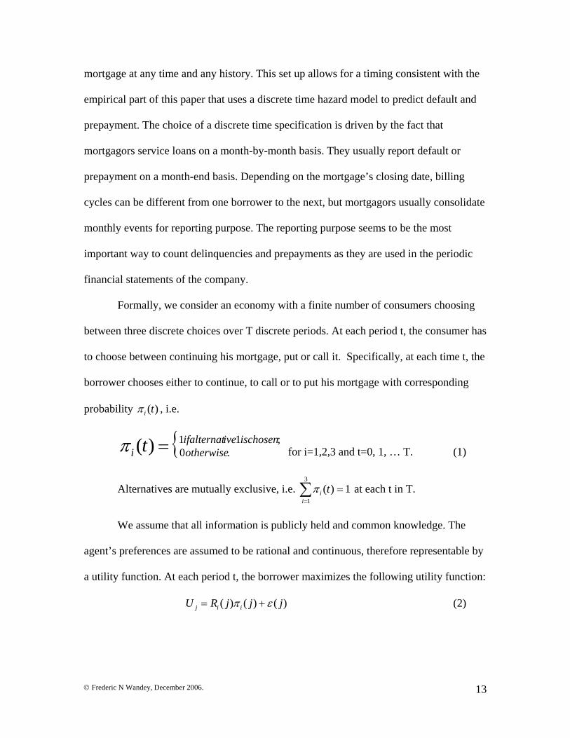
probability )(tiπ , i.e.
{ ;11.0)( ischoseniveifalternat
otherwisei t =π for i=1,2,3 and t=0, 1, … T. (1)
Alternatives are mutually exclusive, i.e. ∑=
=3
1
1)(i
i tπ at each t in T.
We assume that all information is publicly held and common knowledge. The
agent’s preferences are assumed to be rational and continuous, therefore representable by
a utility function. At each period t, the borrower maximizes the following utility function:
)()()( jjjRU iij επ += (2)
© Frederic N Wandey, December 2006.
14
where ))(,),(),(()( jjjHjrjRi φΦ= (3) is the deterministic part of the utility function
representing the cash flow at time j if alternative i is chosen and )( jε is the random error
term representing measurement errors, omitted variables and unaccounted information
about all past and current realizations of the variables that directly or indirectly affect the
value of (2).
The reward )( jRi is a function of the prevailing economic environment
characterized by the idiosyncratic interest rate )( jr 5 and the borrower’s relative position
with regard to local area house price appreciation )( jH . For simplicity, the processes
generating the structure rate and house prices are exogenous to the borrower and depend
on the state of nature. At time j, the borrower makes his decision to put, call or continue
his mortgage based on his knowledge of the current realizations of these variables, not
their entire history.
This assumption is realistic given the fact that the majority of MH borrowers are
in the lower income bracket of the society, with challenged access to information about
past and future interest rates and limited tracking record of house prices appreciation.
These two factors become relevant when borrowers find themselves in a position to
decide about whether to put or call their mortgages. Consequently, only the prevailing
interest rate and house prices are available information when they want to make their
choice.
The borrower’s choice to call or put his mortgage will depend on the information
he has concerning his relative positions with respect to the market interest rates and house
price appreciation. These relative positions are a function of the prevailing market 5 This has to be thought as a spot interest rate for this specific borrower which is function of both the prevailing market rates and both borrower and collateral specific characteristics.
© Frederic N Wandey, December 2006.
15
interest rate, the house price appreciation and idiosyncratic differences across borrowers
represented by the history strings of individual past payment choices summarized by their
current FICO score. The borrower’s position with regard to the prevailing market rates is
captured by the borrower refinance incentive; i.e. the change in gap between the coupon
rate on his mortgage and the market interest rate evaluated at each time he faces the
decision to call or put his mortgage. House price appreciation depends on the status of the
housing market in general, the characteristics of the home and the area in which it is
located. Its movement determines change in loan-to-value ratio and the borrower’s equity
position. High house price appreciation leads to a decrease in the proportion of the value
of the collateral needed to extinguish the debt and to an increase in the investment equity.
Under these circumstances, borrowers are supposed to hold onto their asset. The opposite
situation is more conducive to default.
The last element in the reward function is )( jj zφ , a vector of other collateral
characteristics determined in part by the borrower’s creditworthiness and in part by the
property characteristics; i.e. type (land-home or chattel), age (new or used), width (single
or double-wide), and geographic location6.
6 Given that the lender has already funded the loan, his problem is a Stackelberg-like problem whose optimal solution depends on his ability to foresee borrowers’ choices to put or call the mortgage. The lender’s problem is therefore to maximize the following profit function:
⎪⎩
⎪⎨⎧∑
∑=
−−+
−+
=
=
;)()()(()1(
1
.)()(()1(
10
0
)(tayopeniftheloanstIPtVPtP
r
otherwisetNCPtPr
i
t
tt
t
tt
tπ
where P(t) is the loan repayment amount at time t, VP(t) is the voluntary prepayment by the borrower, IP(t) is any cost due to involuntary prepayment (default), and NCP(t) is the net cost of prepayment if the loan closes at time t by either prepaying or defaulting. Therefore good predictions of voluntary and involuntary prepayment are crucial to the determination of a loan’s cash flow and therefore its pricing.

© Frederic N Wandey, December 2006.
16
To estimate the parameter of the reward function, the present study uses survival
analysis (See Lancaster, 1990; Hosmer, D. W. and Stanley Lemeshow, 1999) to estimate
the probability of an event occurring next period, conditional on the event not having
occurred up to the current period. At each point of time, the model is estimating the
probability for a loan to prepay (default) next period, conditional on it surviving on the
books up to now and not having defaulted (prepaid) yet.
Survival methods have been extensively used in econometric studies having the
following three characteristics. First, the empirical model estimates the expected time
before a well-defined event occurs. Second, observations are right censored. Right
censoring occurs because the event time and type are unknown for individuals for which
the event has not yet occurred at the outcome period. In this case, the event outcome is
set equal to non event. Third, there are explanatory variables that affect the probability of
the occurrence of the studied event. In summarizing survival analysis, two functions are
of central interest: the survival function and the hazard function. Survival function is
concerned with the expected time T until the event occurs.
Let T be a non-negative random variable representing the waiting time until the
occurrence of an event. Assume T is a continuous random variable with probability
density function (p.d.f.) f(t) and cumulative distribution function (c.d.f) given by F(t) =
Pr{T = t}, giving the probability that the event has occurred by duration t. The survivor
function is the probability that the survival time, i.e. the period of time from the time
origin to the occurrence of the event at time t, is greater than or equal to t, i.e.
)(1)Pr()( tFtTtS −=== (4)
For example, the survivor function represents the probability that a loan stays open in

© Frederic N Wandey, December 2006.
17
books from its origination to some time beyond t. The hazard function is the probability
that a loan closes at time t, conditional on it staying open up to t. Formally, the hazard
function can be represented as follows:
htThtTtt h /)|Pr(lim)( 0 ≥+<≤= →λ
= )()(
tStf (5)
The hazard function represents the instantaneous termination rate of a loan at time t,
given that they stayed open until t (Kiefer, 1988). This study will not be looking at the
survival function. It will instead focus on the hazard function. Still, expression (5) shows
clearly that they are closely related.
The reward function )( jRi is actually determined by unobserved latent variables
that are function of variables in expression (3) here represented by the vector z such that
ezjR ii += β')(* .
The following multinomial logit (MNL) model gives the estimated probability to
default (or prepay) for an MH loan during the jth quarter, given the corresponding reward
function represented by the covariates’ vector Z and the fact that no prepayment (or
default) has occurred prior to quarter j:
Prob∑=
+== 2
1
'
'
1)|1)((
1
i
z
z
itiit
it
e
ezntorprepaymedefaultβ
β
(6)
The choice for multinomial specification for the hazard function was guided by
theoretical and empirical reasons. The choice set in the case of the MH prepayment and
default satisfies the property of irrelevant of independent alternatives. The Independence
of Irrelevant Alternatives (IIA) assumption states that the relative odds between any two

© Frederic N Wandey, December 2006.
18
outcomes are independent of the number and nature of other outcomes being
simultaneously considered (McFadden, 1974; Luce, 1959). The clearest case of a
violation of this property is when certain outcomes serve as substitutes for others.
Multinomial logistic regression assumes that none of the categories can serve as
substitutes. If they can serve as substitutes, then the results of multinomial logistic
regression might not be very realistic. In the case of MH loans, most borrowers have
basically a choice between refinancing the existing loan to a different lender to prepay the
existing one or default on the loan. Any other types of transfer of property right
conducted as part of loss mitigation have been excluded from the modeling data.
Moreover, multinomial logit is best suited for predicting events that occur at regular,
discrete points in time, and with large data sets and time-dependent covariates (Allison,
2005).
The hazard model is estimated using the maximum likelihood estimation method
with the caveat that a special accommodation is needed given that the study is using a
mixed sample composed of seasoned and newly originated loans. As in Berger and Black
(1998), newly originated loans permits to recover the parameters associated with new
loans, with an associated disadvantage that this approach limits the observable survival
time to the duration of the panel data (here up to a maximum of twenty one quarters). By
using a mixture of new and seasoned loans, this problem can be avoided. Such a sample
is informative about the hazard function in excess of the twenty one quarters spanning
from September 1999 to January 2005. While a mixed sample of flow- and stock-
sampled observations allows the identification of the hazard function for both long and
© Frederic N Wandey, December 2006.
19
short spells, the use of a mixed sample requires us to adjust the likelihood function to
reflect the presence of stock-sample observations.
This adjustment can be difficult when the origination date of the stock-sampled
loans is unknown7. Fortunately, we know the beginning date of the stock-sampled loans
in our data, which as in Berger and Black (1998) makes the problem more tractable.
Following Berger and Black (1998) let the density function of durations given by
),,( βztf (7)
where t is the duration of the spell, z is a vector of (time-invariant) covariates, and β is a
vector of parameters. Importantly, we assume that ),,( βztf does not vary over time. If
we have a sample of n observations, {t1, t2, . . ., tn}, the likelihood function of the
sample is
∏=
=n
iii ztfL
1
),,()( ββ (8).
To introduce stock sampling, let the set C be the set of loans that were in progress
at the truncation date. For these observations, we know that the loan has stayed open for
r quarters before the panel begins so that the probability that the total survivor time will
be t, given that the spell has lasted until time r, is simply given by
),,(),,(
ββ
zrSztf (9),
7 Klerman (1992) and Swartz, Marcotte, and McBride (1993b) use mixed samples from the SIPP to estimate spells without health insurance when the date the spell began is unknown. Also see Lancaster (1991) for a discussion of the estimation of duration models when the date the spell begins is unknown.
© Frederic N Wandey, December 2006.
20
adjusting these observations by the conditional probability of the loan having stayed open
for r quarters at the beginning of the observation period. Therefore the likelihood
function for the stock- and flow-sample observations combined may be written as
∏∏ ∏∈∈ ∪∈
××=Ci ii
ii
Ai BAiiiii zrS
ztfztSzthL),,(),,(),,(),,()(
βββββ (10).
Convert the last term in equation (10) to a hazard function, the likelihood function
becomes
∏∏ ∏∈∪∈ ∪∪∈
××=Ci iiCAi CBAi
iiii zrSztSzthL
),,(1),,(),,()(
ββββ (11).
As explained in Berger and Black (1998), the third term of the right-hand side of
equation (11) reflects the adjustment necessary for the stock sample. It is an artifact of the
sampling strategy, allowing estimating the underlying parameters of ),,( βztf while
conditioning on r. The likelihood function for a sample of n independent observations
and two competing risks is given by:
∑∑∑∈∈∈
++=n
CUDi iii
n
AUBUCUDiii
n
AUCii xrS
xtSxthBL),,(
1),,(),,()(β
ββ (12)
which can be interpreted as three types of contributions to the probability that a loan
terminates at quarter t or later by either defaulting or prepaying, conditional on that same
loan having survived t quarters in the books (t + r quarters for the stock sample
observation) and not having prepaid or defaulted yet.
© Frederic N Wandey, December 2006.
21
3. Data The development sample is composed of MH proprietary loan-level data from a
servicing company. It includes loans funded between July 1995 and December 2003.
Two types of censoring and a truncation are applied to the data. First, loans with an open
date prior to July 1995 are left-censored from the development sample due to reliability
issues. July 1995 corresponds indeed to the implementation of an in-house data
warehouse system under which loans were better tracked and serviced. Second, the
outcome period is set to January 31, 2005. Data are therefore right censored at that date,
meaning that accounts still open on January 31, 2005 are set to non-event even if they
happen to close in the following months.
Finally, the dataset is truncated as of January 1, 1999 due to the availability of
refreshed FICO8 scores. The FICO score is considered in the loan industry as a summary
of the overall credit worthiness of a consumer. The score is a summation of points given
to a customer based on where the consumer stands in regards to key factors correlated
with delinquency such as status of existing trades with other creditors, ratio of the
balance of trade to credit limit, number of trades, income, assets, etc. Points are
determined based on corresponding factors’ estimated odds ratios. This score can change
from one period to the other depending on the way it is affected by the customer’s debt
payment history and overall credit profile. Therefore, updating the FICO score as time
goes is crucial to improving the predictability of this variable in the model. This is why
8 A FICO score is a credit score developed by Fair Isaac & Co. Credit scoring is a method of determining the likelihood that credit users will be ninety days or more past due twenty-four months into the contract. Fair, Isaac began its pioneering work with credit scoring in the late 1950s and, since then, scoring has become widely accepted by lenders as a reliable means of credit evaluation. A credit score attempts to condense a borrower’s credit history into a single number.

© Frederic N Wandey, December 2006.
22
FICO score enter the model as a time-varying factor, meaning that its value is updated at
each point of time.
The truncation date corresponds to the date at which the considered company
adopted the policy of updating FICO scores on a regular basis. Starting in January 1999,
customers’ credit bureau information is refreshed every month. About a third of the
accounts on the books get refreshed each month such that every single account gets
refreshed at least once every quarter. The left truncation of the data set is the major
difference between a model for newly originated loans and a model for seasoned
accounts. In the first model, every account at the observation date is a newly originated
loan. Default and prepayment are predicted from age zero onwards. Subsequently, loans
still open at each point of time are of the same age. By left truncating the development
sample on September 1, 1999, loans with an open date prior to September 1999 enter the
development sample at their age as of the truncation date, provided that they are still open
at this date. Loans open between October 1999 and December 2003 enter the
development sample at zero months on books whenever they are funded. The
development sample contains both seasoned loans that are not left-censored and newly
originated loans during the observation period. This is an analysis using flow and stock
samples requiring a special specification for the likelihood function as will be made
explicit in section 4 below.

© Frederic N Wandey, December 2006.
23
Figure 3-1 Loan Transition States9
Figure 3-1 above shows different states in which an account can transit before
closing by either defaulting or prepaying. When funded, a loan is current until the
borrower does not send a payment within thirty days after his payment is due. If this
happens to be the case, the account becomes thirty days past due and can transition back
to current if the borrower sends in two payments in the following month. If only one
payment is received, the account stays in the 30 days bucket. If no payment is sent in the
following month, the account rolls into 60 days past due. If still no payment is sent in the
following months, the account will roll further into delinquency until the servicer decides
to proceed to foreclosure. When the loan is in foreclosure, four things can happen. The
mortgagor can repossess the real estate backing the mortgage (REO), ask the borrower to
9 PIF means that the outstanding balance is Paid in full; C means that the account is current; 30, 60, 90 and 120+ stand for 30, 60, 90 and 120+ days past due; FC stands for foreclosure; REO means repossession; SPO, TPS, WO, and SOLD are different types of resolution out of foreclosure decided by the servicer who can agree to let the borrower sale the property himself and pay back
PIF
C30 60 90
120+
FCREO
SPO TPS WO
SOLD
© Frederic N Wandey, December 2006.
24
come up with the outstanding balance to short payoff the loan (SPO), work out a time for
the borrower to sell the house and payoff the loan from the proceeds of the sale (TPS), or
just write off the loan as a complete loss (WO). If the lender decides to repossess the
home, he can either sell the house or, as a loss mitigation strategy for the specific asset
class in consideration, work with the defaulted borrower to find another person to transfer
the contract to. The latest strategy is called detrimental transfer of equity. Under this
mechanism, the new person takes the contract where the first borrower left it by
compensating the first borrower for any equity earned in the house and commit himself
vis-à-vis the lender to honor the mortgage for the rest of the term.
The present study does not model resolutions out of foreclosure because these
decisions are not borrower’s choices. They are loan servicing decisions. This study
focuses on borrower’s behavior by predicting the borrower’s decision to either default or
prepay, conditional on him/her not having prepaid (or defaulted) yet up to this time. The
predicted events are default or prepayment defined as follows. Default means foreclosure
subsequent to default. Prepayment is the borrower’s choice to pay the outstanding
balance in full before the scheduled maturity date. In the specific case of manufactured
homes, prepayments are mostly refinances, i.e. cases where borrowers open a new loan
with another lender with better conditions to payoff the existing loan and reduce the
monthly repayment of the loan.
The following accounts have been excluded from the development sample. First,
loans that have been sold to other financial companies are excluded from the
development sample. These loans are shown in the books as prepayments even though
they are not. Also, loans with terms greater than 360 months have been excluded from the
© Frederic N Wandey, December 2006.
25
development sample, the reason being that such a term is faulty. The company has never
disbursed a loan with a term greater than 360 months.
Given that manufactured homes are of two types, the development sample is first
divided by product type into chattel and land-home loans. Land-home loans fund the
purchase of both the manufactured home and the land on which the house will be placed.
This type of loan is close to the conventional residential mortgage by its terms, collateral
value and performance, as will be shown later. Chattel loans fund only the home, which
can be placed either on privately owned land (non park) or in a trailer park (park).
Chattels, especially park homes, are the most widely known type of manufactured homes
that people have in mind when they refer to manufactured housing. They are supposed to
depreciate over time, leading to poor credit performance and slow prepayment speed. The
empirical part of this paper will compare estimates from these two populations and test
for differences between them. For model validation, each of the two populations is split
2/3 for model development and 1/3 for model validation.
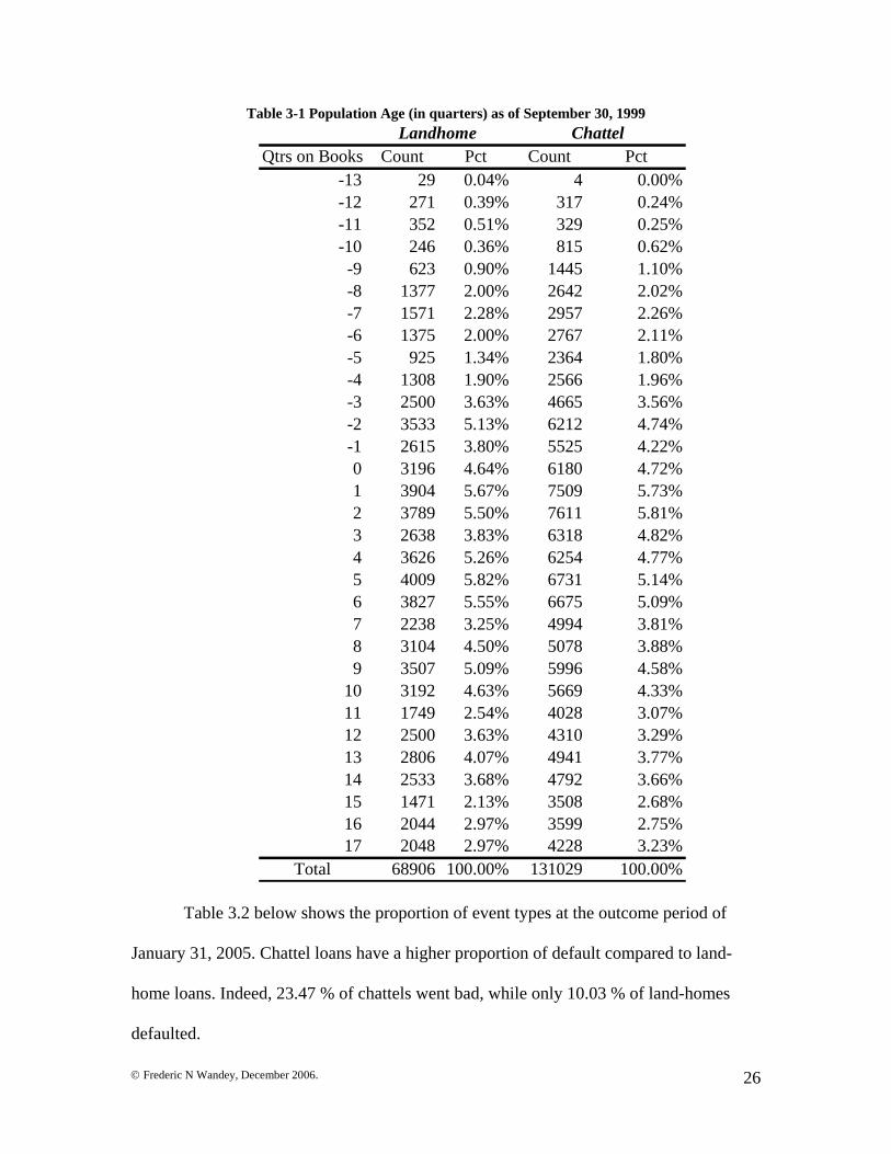
Table 3.1 below provides a snapshot of the modeling data by age (quarters on
books) and origination year as of the truncation date of September 30, 1999. Loans with
negative numbers are loans that are not yet open as of September 30, 1999. They enter
the modeling data at the given number of months after the truncation date. Even though
the population size between chattel and land-home loans is different, the proportion of
loans falling in each quarter bucket is very similar. However, the default and prepayment
distributions are different.
© Frederic N Wandey, December 2006.
26
Table 3-1 Population Age (in quarters) as of September 30, 1999 Landhome Chattel
Qtrs on Books Count Pct Count Pct-13 29 0.04% 4 0.00%-12 271 0.39% 317 0.24%-11 352 0.51% 329 0.25%-10 246 0.36% 815 0.62%
-9 623 0.90% 1445 1.10%-8 1377 2.00% 2642 2.02%-7 1571 2.28% 2957 2.26%-6 1375 2.00% 2767 2.11%-5 925 1.34% 2364 1.80%-4 1308 1.90% 2566 1.96%-3 2500 3.63% 4665 3.56%-2 3533 5.13% 6212 4.74%-1 2615 3.80% 5525 4.22%0 3196 4.64% 6180 4.72%1 3904 5.67% 7509 5.73%2 3789 5.50% 7611 5.81%3 2638 3.83% 6318 4.82%4 3626 5.26% 6254 4.77%5 4009 5.82% 6731 5.14%6 3827 5.55% 6675 5.09%7 2238 3.25% 4994 3.81%8 3104 4.50% 5078 3.88%9 3507 5.09% 5996 4.58%
10 3192 4.63% 5669 4.33%11 1749 2.54% 4028 3.07%12 2500 3.63% 4310 3.29%13 2806 4.07% 4941 3.77%14 2533 3.68% 4792 3.66%15 1471 2.13% 3508 2.68%16 2044 2.97% 3599 2.75%17 2048 2.97% 4228 3.23%
Total 68906 100.00% 131029 100.00%
Table 3.2 below shows the proportion of event types at the outcome period of
January 31, 2005. Chattel loans have a higher proportion of default compared to land-
home loans. Indeed, 23.47 % of chattels went bad, while only 10.03 % of land-homes
defaulted.
© Frederic N Wandey, December 2006.
27
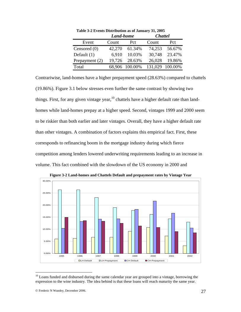
Table 3-2 Events Distribution as of January 31, 2005 Land-home Chattel
Event Count Pct Count PctCensored (0) 42,270 61.34% 74,253 56.67%Default (1) 6,910 10.03% 30,748 23.47%Prepayment (2) 19,726 28.63% 26,028 19.86%Total 68,906 100.00% 131,029 100.00%
Contrariwise, land-homes have a higher prepayment speed (28.63%) compared to chattels
(19.86%). Figure 3.1 below stresses even further the same contrast by showing two
things. First, for any given vintage year,10 chattels have a higher default rate than land-
homes while land-homes prepay at a higher speed. Second, vintages 1999 and 2000 seem
to be riskier than both earlier and later vintages. Overall, they have a higher default rate
than other vintages. A combination of factors explains this empirical fact. First, these
corresponds to refinancing boom in the mortgage industry during which fierce
competition among lenders lowered underwriting requirements leading to an increase in
volume. This fact combined with the slowdown of the US economy in 2000 and
Figure 3-2 Land-homes and Chattels Default and prepayment rates by Vintage Year
0.00%
5.00%
10.00%
15.00%
20.00%
25.00%
30.00%
1995 1996 1997 1998 1999 2000 2001 2002
LH Default LH Prepayment CH Default CH Prepayment
10 Loans funded and disbursed during the same calendar year are grouped into a vintage, borrowing the expression to the wine industry. The idea behind is that these loans will reach maturity the same year.

© Frederic N Wandey, December 2006.
28
2001 led to higher default rate in the 1999 and 2000 cohort of MH loans, especially for
chattel loans.
Table 3.3 below provides the summary statistics of the borrowers and collateral
characteristics for land-home and chattel loans. On average, chattel borrowers have a
lower FICO score (632) than land-home borrowers (638). They have higher loan-to-value
ratio (90%) compared to land-homes (86%). Consequently, they carry a higher coupon
rate (11.58%) than land-home borrowers (8.73%), with a higher interest-coupon rates
spread at origination (3.71 versus 0.83).
Table 3-3 Development Samples Summary Statistics for Land-home and Chattel Populations Group Loan Count Variable Definition Mean Std Dev Minimum Maximum
Land-Home 68,906 CFICO Customer's current FICO score 638 64.5120088 450 836ORIG_LTV Original loan-to-value ratio 85.70 10.4836132 50 100LOANAMT Loan's original balance 79,234$ 26798.17 7666.32 309668.65INTRAT Loan's coupon rate 8.73 1.5074509 1 17.75TERM Loan's term in months 347 39.5884991 60 360QONBOOKS Loan's age in quarters 24 7.2471385 0 38ADJSAL Customer's adjusted monthly salary 3,429$ 1423 1000 10000SATO Interest-coupon spread based on 30-yr Freddie rate 0.83 1.6054855 -5.47 10.78LOSSMIT Indicator for accounts ever loss mitigated 23.50% 0.4240303 0 1DOUBLE Indicator for double-wide home 87.54% 0.330298 0 1NEW Indicator for newly built home 87.28% 0.3332125 0 1CALI Indicator for home located in California 1.74% 0.1308679 0 1
Chattel 131,029 CFICO Customer's current FICO score 632 72.0345968 418 840ORIG_LTV Original loan-to-value ratio 89.62 7.7771992 50 100LOANAMT Loan's original balance 35,525$ 16036.47 5149 248101INTRAT Loan's coupon rate 11.58 2.1156049 0 18TERM Loan's term in months 278 84.8886185 36 360QONBOOKS Loan's age in quarters 23 7.798516 0 38ADJSAL Customer's adjusted monthly salary 3,026$ 1469.55 1000 10000SATO Interest-coupon spread based on 30-yr Freddie rate 3.71 2.2361225 -8.01 12.26LOSSMIT Indicator for accounts ever loss mitigated 21.45% 0.4104501 0 1DOUBLE Indicator for double-wide home 48.02% 0.499609 0 1NEW Indicator for newly built home 58.50% 0.4927275 0 1CALI Indicator for home located in California 5.92% 0.2359489 0 1
Land-home loans on average have a higher balance ($79,234 compared to
$35,525); they have longer terms (347 versus 278 months); they are in larger proportion
double-wide (88% compared to 48%) and new (87% versus 59%). Finally, land-home
borrowers have a higher monthly income ($3,429) than chattel borrowers ($3,026).

© Frederic N Wandey, December 2006.
29
Based on the statistics above, chattel loans can be assumed to be riskier than land-
home loans, while the latter can be assumed to prepay faster than chattel loans. Figures
3.2 and 3.3 below show the empirical hazards by age for land-home and chattel loans
respectively. The empirical hazard is the termination rate of the loans when the only
control factor is time on books. It is computed using the life-table method (see Allison,
2005) grouping event time into intervals starting from 0 to 38 quarters on books (the
longest survival time of a loan in the data set) by an increment of two. The graph in
figure 3.2 and 3.3 shows the conditional probability that a loan will terminate by
prepaying or defaulting, given that it has survived up to the beginning of that quarter. For
each age (quarter on book) the point in the graph is the ratio of loans of that age that
actually close that quarter divided by the population of the same age still at risk of
terminating. The x-axis displays a concatenation of the age (quarter on books) and the
population at risk, while the y-axis displays the exit rate. The top curve is just a
Chattel Empirical Hazard Rates by Quarter on Books
0.00%
0.50%
1.00%
1.50%
2.00%
2.50%
3.00%
0_21
4935
5
2_20
6267
5
4_19
4862
8
6_18
1390
9
8_16
6169
1
10_1
4976
51
12_1
3234
51
14_1
1447
94
16_9
6542
1
18_7
8864
6
20_6
2456
6
22_4
8129
1
24_3
5877
4
26_2
5870
3
28_1
7826
0
30_1
1615
7
32_6
8943
34_3
5835
36_1
3774
38_2
504
Qtrs On Books_Population At Risk
Empirical Default Rate by Age Empirical Prepay Rate by Age Empirical Termination Rate by Age

© Frederic N Wandey, December 2006.
30
combination of the two sub-hazard rates, each of them providing the rates of accounts
closing by defaulting and those closing by prepaying.
Comparing the empirical hazards for the two product-types, we can see that at
comparable age land-home loans have a lower default rate than chattels while chattels
have a lower prepayment rate than land-homes. This confirms the finding documented
previously, i.e. chattel loans are riskier on the credit side while land-home loans are faster
on the prepayment side.
4. Estimation Results Hazard functions have been used to estimate the probability for a manufactured
housing loan to close in the next quarter by prepaying (or defaulting), conditional on it
having survived up to this quarter and not having defaulted (or prepaid) yet. The hazard
function is specified as a discrete-time logistic function, controlling for the age of the
loan, the borrower’s credit quality given by the FICO score and interest rate spread at
LandHome Empirical Hazard Rates by Quarter on Books
0.00%
0.50%
1.00%
1.50%
2.00%
2.50%
3.00%
3.50%
0_12
1747
4
2_11
7126
8
4_11
1106
0
6_10
3792
0
8_95
2970
10_8
5913
7
12_7
5833
0
14_6
5329
2
16_5
4755
0
18_4
4330
9
20_3
4674
9
22_2
6341
2
24_1
9291
1
26_1
3552
7
28_9
0786
30_5
7409
32_3
3100
34_1
6732
36_6
271
38_1
083
Qtrs On Books_Population At Risk
Empirical Default Rate by Age Empirical Prepay Rate by Age Empirical Termination Rate by Age
© Frederic N Wandey, December 2006.
31
loan’s origination11 (SATO), the loan amount, the borrower’s monthly income, his
idiosyncratic position with respect to market interest rates and local house price
appreciation. The borrower’s refinance incentive measures his relative position with
respect to interest rate and is computed as the change in spread between the loan’s
coupon and market interest rate from origination to the current quarter. Local area house
price indices are used to compute market-to-market values for loan-to-value ratio and
borrowers’ equity positions. The interest rate environment is also modeled by adding the
yield curve to the model. The yield curve is defined as the difference between long-term
interest rate (30-year Freddie mortgage rate) and short-term interest rate (1-year Freddie
mortgage rate). Indicators for new homes, doublewide homes, 1999 and 2000 vintage
years, and a California indicator are added to the model.
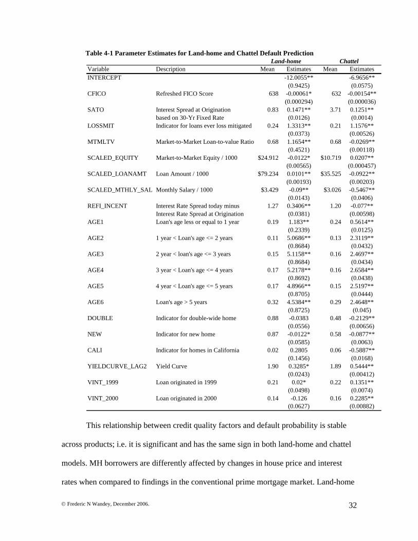
Tables 4-1 and 4-2 below provide side by side estimates for land-home and
chattel default and prepayment predictions. On the credit side (table 4-1), borrowers with
relatively poor credit are more likely to default. Indeed, the lower the FICO score the
more likely the borrower will default. Also, the higher the spread between the loan’s
coupon and the prevailing interest rate at origination the more likely the loan will close
by default. Moreover, loans on which any type of loss mitigation12 policy has been
applied are more likely to default.
11 As lenders use risk-based pricing when originating loans. The spread between the prevailing mortgage rates in the market and the loan’s coupon is indicative of the way the lender perceives the borrower’s risk profile. This spread is added on top of other margin that lenders impose to reflect the fact that mortgages require a lot of servicing, the handling of the monthly payment of principal, interest, and escrow amounts. 12
© Frederic N Wandey, December 2006.
32
Table 4-1 Parameter Estimates for Land-home and Chattel Default Prediction Land-home Chattel
Variable Description Mean Estimates Mean EstimatesINTERCEPT -12.0055** -6.9656**
(0.9425) (0.0575)CFICO Refreshed FICO Score 638 -0.00061* 632 -0.00154**
(0.000294) (0.000036)SATO Interest Spread at Origination 0.83 0.1471** 3.71 0.1251**
based on 30-Yr Fixed Rate (0.0126) (0.0014)LOSSMIT Indicator for loans ever loss mitigated 0.24 1.3313** 0.21 1.1576**
(0.0373) (0.00526)MTMLTV Market-to-Market Loan-to-value Ratio 0.68 1.1654** 0.68 -0.0269**
(0.4521) (0.00118)SCALED_EQUITY Market-to-Market Equity / 1000 $24.912 -0.0122* $10.719 0.0207**
(0.00565) (0.000457)SCALED_LOANAMT Loan Amount / 1000 $79.234 0.0101** $35.525 -0.0922**
(0.00193) (0.00203)SCALED_MTHLY_SAL Monthly Salary / 1000 $3.429 -0.09** $3.026 -0.5467**
(0.0143) (0.0406)REFI_INCENT Interest Rate Spread today minus 1.27 0.3406** 1.20 -0.077**
Interest Rate Spread at Origination (0.0381) (0.00598)AGE1 Loan's age less or equal to 1 year 0.19 1.183** 0.24 0.5614**
(0.2339) (0.0125)AGE2 1 year < Loan's age <= 2 years 0.11 5.0686** 0.13 2.3119**
(0.8684) (0.0432)AGE3 2 year < loan's age <= 3 years 0.15 5.1158** 0.16 2.4697**
(0.8684) (0.0434)AGE4 3 year < Loan's age <= 4 years 0.17 5.2178** 0.16 2.6584**
(0.8692) (0.0438)AGE5 4 year < Loan's age <= 5 years 0.17 4.8966** 0.15 2.5197**
(0.8705) (0.0444)AGE6 Loan's age > 5 years 0.32 4.5384** 0.29 2.4648**
(0.8725) (0.045)DOUBLE Indicator for double-wide home 0.88 -0.0383 0.48 -0.2129**
(0.0556) (0.00656)NEW Indicator for new home 0.87 -0.0122* 0.58 -0.0877**
(0.0585) (0.0063)CALI Indicator for homes in California 0.02 0.2805 0.06 -0.5887**
(0.1456) (0.0168)YIELDCURVE_LAG2 Yield Curve 1.90 0.3285* 1.89 0.5444**
(0.0243) (0.00412)VINT_1999 Loan originated in 1999 0.21 0.02* 0.22 0.1351**
(0.0498) (0.0074)VINT_2000 Loan originated in 2000 0.14 -0.126 0.16 0.2285**
(0.0627) (0.00882)
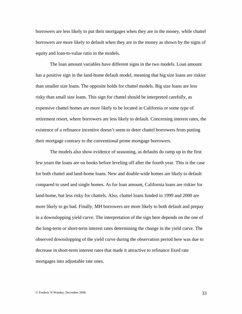
This relationship between credit quality factors and default probability is stable
across products; i.e. it is significant and has the same sign in both land-home and chattel
models. MH borrowers are differently affected by changes in house price and interest
rates when compared to findings in the conventional prime mortgage market. Land-home
© Frederic N Wandey, December 2006.
33
borrowers are less likely to put their mortgages when they are in the money, while chattel
borrowers are more likely to default when they are in the money as shown by the signs of
equity and loan-to-value ratio in the models.
The loan amount variables have different signs in the two models. Loan amount
has a positive sign in the land-home default model, meaning that big size loans are riskier
than smaller size loans. The opposite holds for chattel models. Big size loans are less
risky than small size loans. This sign for chattel should be interpreted carefully, as
expensive chattel homes are more likely to be located in California or some type of
retirement resort, where borrowers are less likely to default. Concerning interest rates, the
existence of a refinance incentive doesn’t seem to deter chattel borrowers from putting
their mortgage contrary to the conventional prime mortgage borrowers.
The models also show evidence of seasoning, as defaults do ramp up in the first
few years the loans are on books before leveling off after the fourth year. This is the case
for both chattel and land-home loans. New and double-wide homes are likely to default
compared to used and single homes. As for loan amount, California loans are riskier for
land-home, but less risky for chattels. Also, chattel loans funded in 1999 and 2000 are
more likely to go bad. Finally, MH borrowers are more likely to both default and prepay
in a downslopping yield curve. The interpretation of the sign here depends on the one of
the long-term or short-term interest rates determining the change in the yield curve. The
observed downslopping of the yield curve during the observation period here was due to
decrease in short-term interest rates that made it attractive to refinance fixed rate
mortgages into adjustable rate ones.

© Frederic N Wandey, December 2006.
34
Table 4-2 Parameter Estimates for Land-home and Chattel Prepayment Prediction Land-home Chattel
Variable Description Mean Estimates Mean EstimatesINTERCEPT -7.2029** -6.3165**
(0.2446) (0.0503)CFICO Refreshed FICO Score 638 0.00297** 632 0.00303**
(0.000182) (0.000043)SATO Interest Spread at Origination 0.83 0.2483** 3.71 0.0731**
based on 30-Yr Fixed Rate (0.00884) (0.00181)LOSSMIT Indicator for loans ever loss mitigated 0.24 -0.823** 0.21 -1.0912**
(0.0338) (0.0111)MTMLTV Market-to-Market Loan-to-value Ratio 0.68 -2.0477** 10.72 -0.0298**
(0.25) (0.00114)SCALED_EQUITY Market-to-Market Equity / 1000 $24.912 -0.00077 $35.525 0.0104**
(0.00313) (0.000508)SCALED_LOANAMT Loan Amount / 1000 $79.234 0.00416** $3.026 0.1021**
(0.00125) (0.00187)SCALED_MTHLY_SAL Monthly Salary / 1000 $3.429 0.0363** $0.680 -3.3957**
(0.00829) (0.0388)REFI_INCENT Interest Rate Spread today minus 1.27 0.1404** 1.20 -0.4384**
Interest Rate Spread at Origination (0.0241) (0.00692)AGE1 Loan's age less or equal to 1 year 0.19 0.2105** 0.24 0.2556**
(0.0423) (0.00938)AGE2 1 year < Loan's age <= 2 years 0.11 0.9383** 0.13 1.3967**
(0.1299) (0.0293)AGE3 2 year < loan's age <= 3 years 0.15 1.1598** 0.16 1.4942**
(0.1296) (0.0298)AGE4 3 year < Loan's age <= 4 years 0.17 1.3067** 0.16 1.7153**
(0.1311) (0.0305)AGE5 4 year < Loan's age <= 5 years 0.17 1.4463** 0.15 1.9365**
(0.1333) (0.0313)AGE6 Loan's age > 5 years 0.32 1.5089** 0.29 2.2192**
(0.1372) (0.0324)DOUBLE Indicator for double-wide home 0.88 0.6587** 0.48 0.2084**
(0.044) (0.00738)NEW Indicator for new home 0.87 0.1689** 0.58 -0.0683**
(0.0402) (0.0076)CALI Indicator for homes in California 0.02 0.0538 0.06 -0.0709**
(0.0717) (0.0112)YIELDCURVE_LAG2 Yield Curve 1.90 0.0441** 1.89 0.3057**
(0.0138) (0.00413)VINT_1999 Loan originated in 1999 0.21 -0.128** 0.22 0.114**
(0.0343) (0.00886)VINT_2000 Loan originated in 2000 0.14 -0.2097** 0.16 0.2533**
(0.0453) (0.0116) On the speed side, borrowers with better credit prepay faster compared to those
with constrained credit. The FICO score is positively correlated with prepayment.
Moreover, loans on which any type of loss mitigation action was taken are less likely to
close by prepaying. At the same time, some MH borrowers are curing following the
© Frederic N Wandey, December 2006.
35
funding of their mortgage. This is indicated by a positive sign for SATO in the
prepayment models.
SATO reflects lenders’ risk-based pricing of loans at origination. Therefore, the
higher the SATO the riskier the borrower’s profile appears to the lender when originating
the loan. A positive sign for SATO in the prepayment models means that the higher the
SATO the more likely the loan is going to prepay. Given that most of the prepayment
activities for MH loans are streamline refinances, a positive sign for SATO means that
borrowers with high SATO are able to find another lender who can give them a better
deal than the one they currently have. This can happen under two circumstances. The first
likely scenario is that interest rates have been decreasing and the borrower’s credit profile
hasn’t deteriorated. He can therefore go to a different lender and get a lower rate based
only on the change in the interest rate environment13. The second scenario is that interest
rates have not changed but the borrower has significantly improved his debt repayment
behavior. This will increase his/her FICO score, strengthen his/her overall credit profile,
and give him/her access to refinancing options susceptible of reducing his monthly
repayment of the loan. In both scenarios, credit curing, or at least credit not deteriorating,
is the minimal condition to open up new refinancing perspectives to a borrower with high
SATO.
House price appreciation affects prepayment decisions as expected, as borrowers
with low current loan-to-value ratio and built equity14 in their homes are more likely to
prepay. As on the credit side, the refinance incentive does not trigger prepayment for
chattel borrowers. Still, MH borrowers are more likely to prepay under a flattening yield
13 Given that the model controls for changing rate environment with the yield curve and refinance incentive, this first scenario is less plausible. 14 However, equity variable is not significant for land-home borrowers.

© Frederic N Wandey, December 2006.
36
curve, implying that borrowers are swapping short-term interest rates with long-term ones
by refinancing into adjustable rate mortgages.15 Prepayments are likely to increase as
loans season, as shown by the signs and the magnitudes of the age bins in the model.
Double-wide and new MH loans are more likely to prepay; so are land-home loans
booked in 1999 and 2000.
Figure 4-0-1 Land-home & Chattel Actual vs. Expected Default and Prepayment Probabilities by Age
(a) Land-Home Default
0.00%
0.20%
0.40%
0.60%
0.80%
1.00%
1.20%
1.40%
1.60%
1 4 7 8 10 11 12 13 14 16 17 18 19 20 22 23 24 26 29 33
Quarters on books
Rat
e
Actual Default Expected Default
(c) Land-Home Prepayment
0.00%
0.50%
1.00%
1.50%
2.00%
2.50%
3.00%
3.50%
4.00%
1 4 6 8 9 11 12 13 14 15 16 17 19 20 21 22 24 26 28 32
Quarters on books
Rat
e
Actual Prepayment Expected Prepayment
(b) Chattel Default
0.00%
0.50%
1.00%
1.50%
2.00%
2.50%
3.00%
3.50%
1 4 5 7 8 9 11 12 13 14 15 17 18 19 20 22 23 25 28 32
Quarters on books
Rat
eActual Default Expected Default
(d) Chattel Prepayment
0.00%
0.50%
1.00%
1.50%
2.00%
2.50%
3.00%
1 4 5 7 8 9 11 12 13 14 15 17 18 19 20 22 23 25 28 32
Quarters on books
Rat
e
Actual Prepayment Expected Prepayment
Figures 4-1 to 4-3 plot actual versus predicted default and prepayment rates by a
number of variable cuts. The cut by age shows that on average default (Figure 4-1 (a) and
(b)) ramps up steeply from the first quarter and reaches a peak at fourteen quarters on
15 This is a conjecture based on the prepayment behavior observed in the mortgage industry (see …) from the late 90’s until mid-2005, a period during which falling interest rates and the media effect related to it, have led borrowers to refinance their mortgages into new adjustable rates products that have been expanding during these years.
© Frederic N Wandey, December 2006.
37
books. It then decreases a little bit before leveling off. The same figure 4-1 (c and d)
shows that there seems not to be a turning point of prepayment for seasoning MH loans.
In these graphs, average prepayment rates continuously increase as loans season for both
chattel and land-homes.
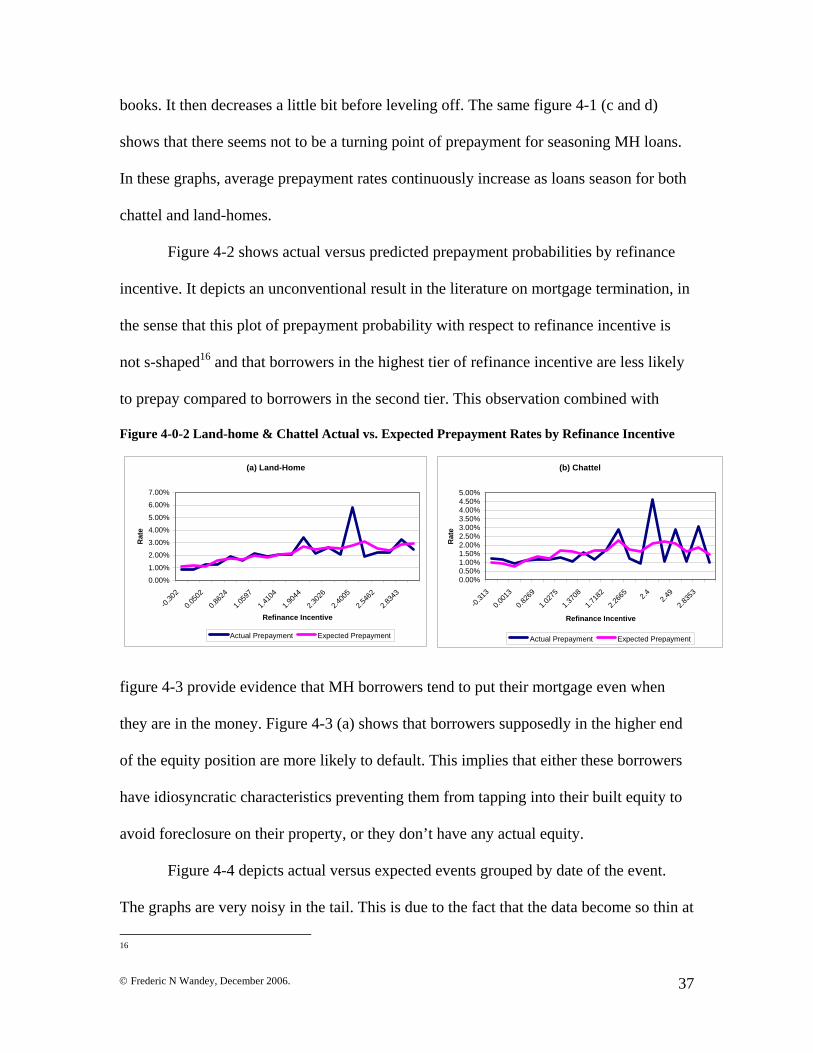
Figure 4-2 shows actual versus predicted prepayment probabilities by refinance
incentive. It depicts an unconventional result in the literature on mortgage termination, in
the sense that this plot of prepayment probability with respect to refinance incentive is
not s-shaped16 and that borrowers in the highest tier of refinance incentive are less likely
to prepay compared to borrowers in the second tier. This observation combined with
Figure 4-0-2 Land-home & Chattel Actual vs. Expected Prepayment Rates by Refinance Incentive
(a) Land-Home
0.00%
1.00%
2.00%
3.00%
4.00%
5.00%
6.00%
7.00%
-0.30
2
0.050
2
0.862
4
1.059
7
1.410
4
1.904
4
2.302
6
2.400
5
2.546
2
2.834
3
Refinance Incentive
Rat
e
Actual Prepayment Expected Prepayment
(b) Chattel
0.00%0.50%1.00%1.50%2.00%2.50%3.00%3.50%4.00%4.50%5.00%
-0.31
3
0.001
3
0.826
9
1.027
5
1.370
8
1.718
2
2.266
5 2.4 2.49
2.835
3
Refinance Incentive
Rat
e
Actual Prepayment Expected Prepayment
figure 4-3 provide evidence that MH borrowers tend to put their mortgage even when
they are in the money. Figure 4-3 (a) shows that borrowers supposedly in the higher end
of the equity position are more likely to default. This implies that either these borrowers
have idiosyncratic characteristics preventing them from tapping into their built equity to
avoid foreclosure on their property, or they don’t have any actual equity.
Figure 4-4 depicts actual versus expected events grouped by date of the event.
The graphs are very noisy in the tail. This is due to the fact that the data become so thin at 16

© Frederic N Wandey, December 2006.
38
Figure 4-0-3 Land-home & Chattel Actual vs. Expected Default and Prepayment Rates by Equity
(a) Land-Home
0.00%
0.20%
0.40%
0.60%
0.80%
1.00%
1.20%
6379 12207 15549 18368 21047 23763 26780 30350 35117 43567
Market-to-Market Equity
Rat
e
Actual Default Expected Default
(b) Chattel
0.00%
0.50%
1.00%
1.50%
2.00%
2.50%
3.00%
2530 4510 5758 6934 8136 9476 11050 13023 15761 20537
Market-to-Market Equity
Rat
e
Actual Default Expected Default
these later date that any event get a relatively higher importance. Moreover, the company
providing the data went through a dramatic change in management that led to picks in
foreclosure and prepayments around the takeover period.
Figure 4-0-4 Actual vs. Expected Default and Prepayment Rates by Quarter
(a) Land-home Default
0.00%0.50%1.00%1.50%2.00%2.50%3.00%3.50%4.00%4.50%
10/1/
1999
4/1/2000
10/1/2000
4/1/20
01
10/1/
2001
4/1/20
02
10/1/
2002
4/1/2003
10/1/2003
4/1/20
04
10/1/
2004
As of Date
Rat
e
Actual Default Expected Default
(c) Land-home Prepayment
0.00%
1.00%
2.00%
3.00%
4.00%
5.00%
6.00%
1999
Q4
2000
Q2
2000
Q4
2001
Q2
2001
Q4
2002
Q2
2002
Q4
2003
Q2
2003
Q4
2004
Q2
2004
Q4
As of Date
Rat
e
Actual Prepayment Expected Prepayment
(b) Chattel Default
0.00%
2.00%
4.00%
6.00%
8.00%
10.00%
12.00%
10/1/1999
4/1/2000
10/1/2000
4/1/2001
10/1/2001
4/1/2002
10/1/2002
4/1/2003
10/1/2003
4/1/2004
10/1/2004
As of Date
Rat
e
Actual Default Expected Default
(d) Chattel Prepayment
0.00%0.50%1.00%1.50%2.00%2.50%3.00%3.50%4.00%4.50%5.00%
1999
Q4
2000
Q2
2000
Q4
2001
Q2
2001
Q4
2002
Q2
2002
Q4
2003
Q2
2003
Q4
2004
Q2
2004
Q4
As of Date
Rat
e
Actual Prepayment Expected Prepayment

© Frederic N Wandey, December 2006.
39
Land home loans behave closer to the conventional mortgage with regard to house
price appreciation and interest rates. The models validation on the development and
holdout sample show an overall better fit of the default predictions than that of the
prepayment one. The accuracy of prepayment prediction is challenged by the fact that
MH borrowers’ prepayment behavior is not always consistent with the theory backing the
choice and definition of mortgages’ prepayments. The difficulty of accurately predicting
Table 4-3 Models Lift and K-S Statistics
Group Sample Lift KS Lift KSLand-home Development 5.09 41.09 4.82 38.41
Holdout 4.32 37.58 4.09 29.52Chattel Development 2.33 26.71 3.34 28.81
Holdout 2.04 22.82 3.08 28.10
Default Prepayment
default and prepayment for these products requires the estimation of a confidence interval
given the importance of borrowers’ prepayment behavior (Spahr and Sunderman, 1998) and
default for mortgage and mortgage-backed securities cash flow valuation.
5. A Confidence Interval for Default and Prepayment Predictions Confidence intervals to default and prepayment predictions were estimated using
confidence interval bootstrapping. Bootstrapping entails random resampling to obtain the
desired empirical distribution of the parameters of interest. One advantage of
bootstrapping is that it usually provides more accurate confidence intervals than the
conventional asymptotic distribution approaches (Mooney and Duval, 1993). Generally,
the 95% confidence interval is computed by adding or subtracting the standard error
multiplied by a critical value (e.g. q ± 1.96sq). This computation assumes that the
confidence interval is symmetric around q and that the estimate of sq is correct. There are
many situations in which the parametric assumptions may be incorrect, and it is useful in
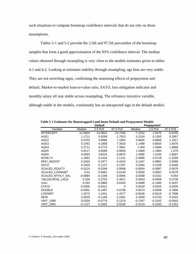
© Frederic N Wandey, December 2006.
40
such situations to compute bootstrap confidence intervals that do not rely on those
assumptions.
Tables 5-1 and 5-2 provide the 2.5th and 97.5th percentiles of the bootstrap
samples that form a good approximation of the 95% confidence interval. The median
values obtained through resampling is very close to the models estimates given in tables
4-1 and 4-2. Looking at estimates stability through resampling, age bins are very stable.
They are not switching signs, confirming the seasoning effects of prepayment and
default. Market-to-market loan-to-value ratio, SATO, loss mitigation indicator and
monthly salary all stay stable across resampling. The refinance incentive variable,
although stable in the models, consistently has an unexpected sign in the default models.
Table 5-1 Estimates for Bootstrapped Land-home Default and Prepayment Models
Default PrepaymentVariable Median 2.5 Pctl 97.5 Pctl Median 2.5 Pctl 97.5 Pctl
INTERCEPT -12.0664 -14.6802 -10.7326 -7.1522 -7.8475 -6.5155AGE1 1.1711 0.9299 1.7913 0.2104 0.1263 0.2957AGE2 5.0702 4.0966 7.1804 0.9605 0.6669 1.1917AGE3 5.1052 4.1858 7.3033 1.1498 0.8835 1.4075AGE4 5.2711 4.2776 7.3561 1.304 1.0494 1.5866AGE5 4.9117 3.9289 6.9926 1.4469 1.1964 1.679AGE6 4.5593 3.6019 6.6876 1.5085 1.2245 1.8057MTMLTV 1.1891 0.1416 2.1131 -2.0686 -2.5718 -1.3258REFI_INCENT 0.3433 0.2477 0.4242 0.1447 0.0881 0.2068SATO 0.1503 0.1127 0.1767 0.2462 0.2238 0.2649SCALED_EQUITY -0.0124 -0.0248 0.0008 -0.0004 -0.0087 0.0079SCALED_LOANAMT 0.01 0.0061 0.0144 0.0039 0.0007 0.0078SCALED_MTHLY_SAL -0.0884 -0.1248 -0.0585 0.0368 0.0161 0.054YIELDCURVE_LAG2 0.326 0.2703 0.3971 0.0453 -0.0009 0.0728CALI 0.292 -0.0883 0.6333 0.0468 -0.1484 0.2037CFICO -0.0005 -0.0012 0 0.0029 0.0025 0.0034DOUBLE -0.0491 -0.1497 0.0738 0.6573 0.5658 0.7806LOSSMIT 1.3272 1.2441 1.4277 -0.8245 -0.9216 -0.7598NEW 0.0035 -0.1199 0.1651 0.1639 0.0743 0.2422VINT_1999 0.0329 -0.0779 0.1374 -0.1347 -0.2162 -0.0542VINT_2000 -0.1127 -0.2663 0.0239 -0.2219 -0.3183 -0.1251
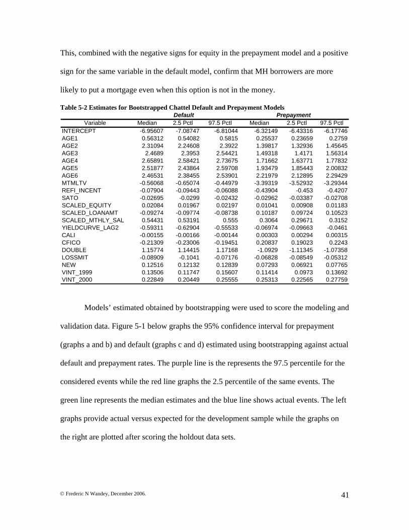
© Frederic N Wandey, December 2006.
41
This, combined with the negative signs for equity in the prepayment model and a positive
sign for the same variable in the default model, confirm that MH borrowers are more
likely to put a mortgage even when this option is not in the money.
Table 5-2 Estimates for Bootstrapped Chattel Default and Prepayment Models Default Prepayment
Variable Median 2.5 Pctl 97.5 Pctl Median 2.5 Pctl 97.5 PctlINTERCEPT -6.95607 -7.08747 -6.81044 -6.32149 -6.43316 -6.17746AGE1 0.56312 0.54082 0.5815 0.25537 0.23659 0.2759AGE2 2.31094 2.24608 2.3922 1.39817 1.32936 1.45645AGE3 2.4689 2.3953 2.54421 1.49318 1.4171 1.56314AGE4 2.65891 2.58421 2.73675 1.71662 1.63771 1.77832AGE5 2.51877 2.43864 2.59708 1.93479 1.85443 2.00832AGE6 2.46531 2.38455 2.53901 2.21979 2.12895 2.29429MTMLTV -0.56068 -0.65074 -0.44979 -3.39319 -3.52932 -3.29344REFI_INCENT -0.07904 -0.09443 -0.06088 -0.43904 -0.453 -0.4207SATO -0.02695 -0.0299 -0.02432 -0.02962 -0.03387 -0.02708SCALED_EQUITY 0.02084 0.01967 0.02197 0.01041 0.00908 0.01183SCALED_LOANAMT -0.09274 -0.09774 -0.08738 0.10187 0.09724 0.10523SCALED_MTHLY_SAL 0.54431 0.53191 0.555 0.3064 0.29671 0.3152YIELDCURVE_LAG2 -0.59311 -0.62904 -0.55533 -0.06974 -0.09663 -0.0461CALI -0.00155 -0.00166 -0.00144 0.00303 0.00294 0.00315CFICO -0.21309 -0.23006 -0.19451 0.20837 0.19023 0.2243DOUBLE 1.15774 1.14415 1.17168 -1.0929 -1.11345 -1.07358LOSSMIT -0.08909 -0.1041 -0.07176 -0.06828 -0.08549 -0.05312NEW 0.12516 0.12132 0.12839 0.07293 0.06921 0.07765VINT_1999 0.13506 0.11747 0.15607 0.11414 0.0973 0.13692VINT_2000 0.22849 0.20449 0.25555 0.25313 0.22565 0.27759
Models’ estimated obtained by bootstrapping were used to score the modeling and
validation data. Figure 5-1 below graphs the 95% confidence interval for prepayment
(graphs a and b) and default (graphs c and d) estimated using bootstrapping against actual
default and prepayment rates. The purple line is the represents the 97.5 percentile for the
considered events while the red line graphs the 2.5 percentile of the same events. The
green line represents the median estimates and the blue line shows actual events. The left
graphs provide actual versus expected for the development sample while the graphs on
the right are plotted after scoring the holdout data sets.
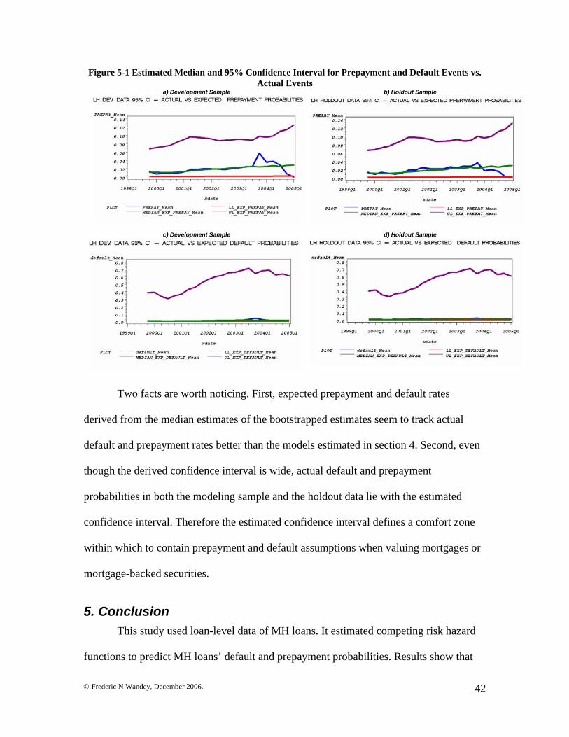
© Frederic N Wandey, December 2006.
42
Figure 5-1 Estimated Median and 95% Confidence Interval for Prepayment and Default Events vs. Actual Events
a) Development Sample b) Holdout Sample
c) Development Sample d) Holdout Sample
Two facts are worth noticing. First, expected prepayment and default rates
derived from the median estimates of the bootstrapped estimates seem to track actual
default and prepayment rates better than the models estimated in section 4. Second, even
though the derived confidence interval is wide, actual default and prepayment
probabilities in both the modeling sample and the holdout data lie with the estimated
confidence interval. Therefore the estimated confidence interval defines a comfort zone
within which to contain prepayment and default assumptions when valuing mortgages or
mortgage-backed securities.
5. Conclusion This study used loan-level data of MH loans. It estimated competing risk hazard
functions to predict MH loans’ default and prepayment probabilities. Results show that
© Frederic N Wandey, December 2006.
43
variables used to capture option price theory in the literature on mortgage termination
affect MH borrowers differently. Land-home borrowers are more likely to behave in a
way consistent with the predictions of the theory, while chattel borrowers are more likely
to put their mortgage even when it is in the money not to do so. The difficulty of
accurately predicting default and prepayment for these products required the estimation
of a confidence interval given the importance of prepayment and default assumption
when forecasting the risk associated to mortgage termination. Interval bootstrapping was
used to estimate robust parameters to the model and derive a 95% confidence interval for
the estimators. Validations’ results not only confirm stability of the parameter estimates
but also show that actual CDR and CPR lie within the estimated confidence intervals.
The next task still to be completed is to validate these results on an out-of-sample data.

© Frederic N Wandey, December 2006.
44
References Allison, Paul D. (2005), Survival Analysis using SAS. A practical Guide. 9th ed., SAS
Institute Inc., Cary, NC, USA.
Ambroze, B. and C. Capone (2000). “The Hazard Rates of First and Second Defaults.
Journal of Real Estate Finance and economics 20, 275-293.
Berger, M. C. and D. A. Black (1998). “The Duration of Medicaid Spells: An Analysis
using Flow and Stock Samples”. Revue of Economics and Statistics 80 (4), Nov,
667-675.
Black, F. and M. Scholes (1973). “The Pricing of Options and Corporate Liabilities”.
The Journal of Political Economy 81 (3), 637-654.
Clement, E., C. Gourieroux and A. Monfort (2000), “Econometric Specification of the
Risk Neutral Valuation Model”. Journal of Econometrics 94, 117-143.
Danis, M. and A. Pennington-Cross (2005a). “The Delinquency of Subprime Mortgages”.
Federal Reserve Bank of St. Louis Working paper 2005-022A, March.
Danis, M. and A. Pennington-Cross (2005b). “A Dynamic Look at Subprime Loan
Performance”. Federal Reserve Bank of St. Louis Working paper 2005-029A,
May.
Deng, Y., John M. Quigley, and R. Van Order (2000). “Mortgage Terminations,
Heterogeneity and The Exercise of Mortgage Options”. Econometrica 68 (2),
275-307.
Dunn K. B. and Kenneth J. Singleton (1983). “An Empirical Analysis of the Pricing of
Mortgage-Backed Securities”. The Journal of Finance 38 (2), Papers and
Proceedings Forty-First Annual Meeting American Finance Association New
York, N.Y. December 28-30, 1982 (May, 1983), pp. 613-623

© Frederic N Wandey, December 2006.
45
Eaton, J., and M. Gersovitz (1981): “Debt with Potential Repudiation: Theoretical and
Empirical Analysis,” Review of Economic Studies 48, 289-309.
Eckstein, Zvi, and Kenneth I. Wolpin (1989): "The Specification and Estimation of
Dynamic Stochastic Discrete Choice Models: A Survey ", Journal of Human
Resources 24, 562-598.
Gjaja, I. M., M. E. Kane and M. Carnahan (2004). “Delinquency Transitions in Subprime
Loans. Analysis, Model, Implications”. Citigroup United States Fixed Income
Research, Asset Backed Securities, March 17, 2004.
Gjaja, I. M., M. E. Kane and M. Carnahan (2005a). “Introduction to the Home Equity
Loan Market”. Citigroup United States Fixed Income Research, Asset Backed and
Mortgage Credit, October 20, 2005.
Gjaja, I. M., O. Beelders and A. Omprakash (2005b). “Subprime Hybrid Prepayments.
Analysis and Model.” Citigroup United States Fixed Income Research, Asset
Backed and Mortgage Credit, December 14, 2005.
Hart, J. F., M. J. Rhodes and J. T. Morgan (2002). The Unknown World of the Mobile
Home. Creating the North American Landscape, Baltimore: The Johns Hopkins
University Press, 142p.
Hendershott, P. H., and R. Van Order (1987). “Pricing Mortgages: An Interpretation of
the Models and Results,” Journal of Financial Services Research 1, 77-111.
Jewell, K. (2003). “Manufactured Housing Appreciation: Stereotypes and Data”.
Consumers Union Southwest Regional Office Consumer Reports, April, 44p.
Kau, James B. and Donald C. Keenan (1995), An Overview of the Option-Theoretic
Pricing of Mortgages. Journal of Housing Research 6 (2), pp. 217-244.

© Frederic N Wandey, December 2006.
46
Kehoe, Timothy J., and David K. Levine (1993): “Debt-Constrained Asset Markets,”
Review of Economic Studies 60, 865-888.
Luce, D. (1959). Individual Choice Behavior. New York: John Wiley and Sons.
Lunneborg, C. E. (2000). Data Analysis by Resampling: Concepts and Applications,
Pacific Grove: Duxbury.
McFadden, D. (1974). “Conditional Logit Analysis of Qualitative Choice Behavior.” In
Frontiers in Econometrics, edited by P. Zarembka, New York: Academic Press,
pp. 105-142.
Mooney, C.Z., and Duval, R.D. (1993). Bootstrapping: A Nonparametric Approach to
Statistical Inference, Sage Publications, Newberry Park, Ca., 21.
Munneke, H. J. and V. Carlos Slawson, Jr. (1999). “A Housing Price Model with
Endogeneous Externality Location: A Study of Mobile Home Parks”. Journal of
Real Estate Finance and Economics 19 (2), 113-131.
Quercia, R. G. and Michael A. Stegman,. “Residential Mortgage Default: A Review of
the Literature”. Journal of Housing Research 3 (2), pp. 341-379.
Sheehan, M. F. and R. D. Colton (1994), “The Problem of Mass Evictions in Mobile
Home Parks Subject to Conversion”. Report.
Spahr, R. W. and Mark A. Sunderman (19 ), “The Effect of Prepayment Modeling in
Pricing Mortgage-Backed Securities.” Journal of Housing Research 3 (2), 381-
400.
VanderHoff, J. (1996). “Adjustable and Fixed Rate Mortgage Termination, Option
Values and Local Market Conditions: An Empirical Analysis.” Real Estate
Economics 24 (3), 379-406.
© Frederic N Wandey, December 2006.
47
Wallis, A. D. (1991). Wheel Estate: The Rise and Decline of Mobile Homes, New York:
Oxford University Press, 283p.
Wood, M. (2003) Making Sense of Statistics: a Non-mathematical Approach.
Basingstoke: Palgrave.
Related Documents