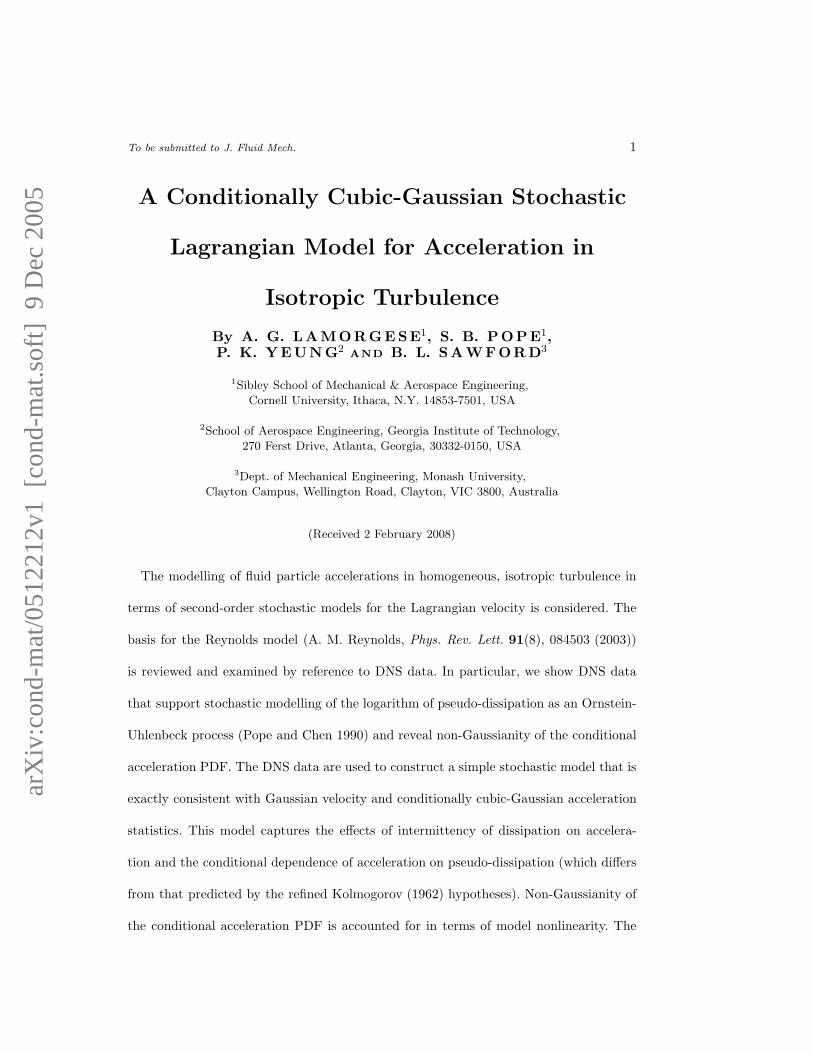
arXiv:cond-mat/0512212v1 [cond-mat.soft] 9 Dec 2005 To be submitted to J. Fluid Mech. 1 A Conditionally Cubic-Gaussian Stochastic Lagrangian Model for Acceleration in Isotropic Turbulence By A. G. LAMORGESE 1 , S. B. POPE 1 , P. K. YEUNG 2 AND B. L. SAWFORD 3 1 Sibley School of Mechanical & Aerospace Engineering, Cornell University, Ithaca, N.Y. 14853-7501, USA 2 School of Aerospace Engineering, Georgia Institute of Technology, 270 Ferst Drive, Atlanta, Georgia, 30332-0150, USA 3 Dept. of Mechanical Engineering, Monash University, Clayton Campus, Wellington Road, Clayton, VIC 3800, Australia (Received 2 February 2008) The modelling of fluid particle accelerations in homogeneous, isotropic turbulence in terms of second-order stochastic models for the Lagrangian velocity is considered. The basis for the Reynolds model (A. M. Reynolds, Phys. Rev. Lett. 91(8), 084503 (2003)) is reviewed and examined by reference to DNS data. In particular, we show DNS data that support stochastic modelling of the logarithm of pseudo-dissipation as an Ornstein- Uhlenbeck process (Pope and Chen 1990) and reveal non-Gaussianity of the conditional acceleration PDF. The DNS data are used to construct a simple stochastic model that is exactly consistent with Gaussian velocity and conditionally cubic-Gaussian acceleration statistics. This model captures the effects of intermittency of dissipation on accelera- tion and the conditional dependence of acceleration on pseudo-dissipation (which differs from that predicted by the refined Kolmogorov (1962) hypotheses). Non-Gaussianity of the conditional acceleration PDF is accounted for in terms of model nonlinearity. The

Welcome message from author
This document is posted to help you gain knowledge. Please leave a comment to let me know what you think about it! Share it to your friends and learn new things together.
Transcript
arX
iv:c
ond-
mat
/051
2212
v1 [
cond
-mat
.sof
t] 9
Dec
200
5
To be submitted to J. Fluid Mech. 1
A Conditionally Cubic-Gaussian Stochastic
Lagrangian Model for Acceleration in
Isotropic Turbulence
By A. G. LAMORGESE1, S. B. POPE1,P. K. YEUNG2
AND B. L. SAWFORD3
1Sibley School of Mechanical & Aerospace Engineering,
Cornell University, Ithaca, N.Y. 14853-7501, USA
2School of Aerospace Engineering, Georgia Institute of Technology,
270 Ferst Drive, Atlanta, Georgia, 30332-0150, USA
3Dept. of Mechanical Engineering, Monash University,
Clayton Campus, Wellington Road, Clayton, VIC 3800, Australia
(Received 2 February 2008)
The modelling of fluid particle accelerations in homogeneous, isotropic turbulence in
terms of second-order stochastic models for the Lagrangian velocity is considered. The
basis for the Reynolds model (A. M. Reynolds, Phys. Rev. Lett. 91(8), 084503 (2003))
is reviewed and examined by reference to DNS data. In particular, we show DNS data
that support stochastic modelling of the logarithm of pseudo-dissipation as an Ornstein-
Uhlenbeck process (Pope and Chen 1990) and reveal non-Gaussianity of the conditional
acceleration PDF. The DNS data are used to construct a simple stochastic model that is
exactly consistent with Gaussian velocity and conditionally cubic-Gaussian acceleration
statistics. This model captures the effects of intermittency of dissipation on accelera-
tion and the conditional dependence of acceleration on pseudo-dissipation (which differs
from that predicted by the refined Kolmogorov (1962) hypotheses). Non-Gaussianity of
the conditional acceleration PDF is accounted for in terms of model nonlinearity. The
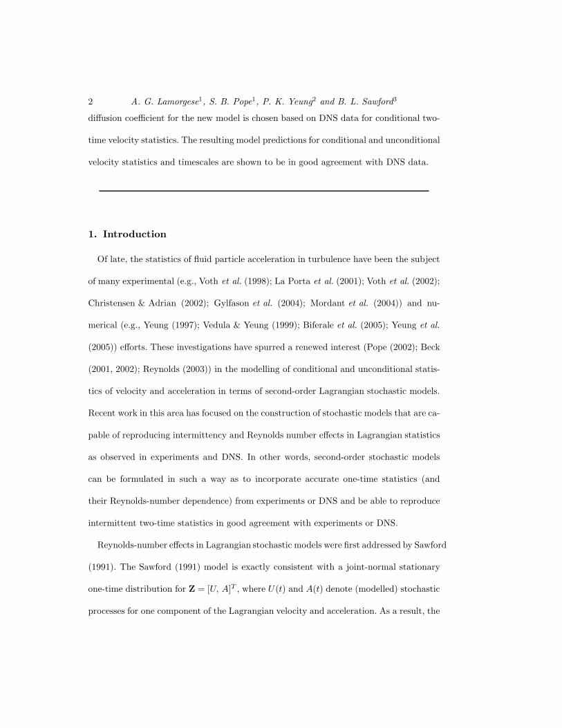
2 A. G. Lamorgese1, S. B. Pope1, P. K. Yeung2 and B. L. Sawford3
diffusion coefficient for the new model is chosen based on DNS data for conditional two-
time velocity statistics. The resulting model predictions for conditional and unconditional
velocity statistics and timescales are shown to be in good agreement with DNS data.
1. Introduction
Of late, the statistics of fluid particle acceleration in turbulence have been the subject
of many experimental (e.g., Voth et al. (1998); La Porta et al. (2001); Voth et al. (2002);
Christensen & Adrian (2002); Gylfason et al. (2004); Mordant et al. (2004)) and nu-
merical (e.g., Yeung (1997); Vedula & Yeung (1999); Biferale et al. (2005); Yeung et al.
(2005)) efforts. These investigations have spurred a renewed interest (Pope (2002); Beck
(2001, 2002); Reynolds (2003)) in the modelling of conditional and unconditional statis-
tics of velocity and acceleration in terms of second-order Lagrangian stochastic models.
Recent work in this area has focused on the construction of stochastic models that are ca-
pable of reproducing intermittency and Reynolds number effects in Lagrangian statistics
as observed in experiments and DNS. In other words, second-order stochastic models
can be formulated in such a way as to incorporate accurate one-time statistics (and
their Reynolds-number dependence) from experiments or DNS and be able to reproduce
intermittent two-time statistics in good agreement with experiments or DNS.
Reynolds-number effects in Lagrangian stochastic models were first addressed by Sawford
(1991). The Sawford (1991) model is exactly consistent with a joint-normal stationary
one-time distribution for Z = [U, A]T , where U(t) and A(t) denote (modelled) stochastic
processes for one component of the Lagrangian velocity and acceleration. As a result, the
Conditionally Cubic-Gaussian Stochastic Lagrangian Model 3
SDEs for the Sawford (1991) model are linear :
dZ =
0 1
−σ2
A
σ2
U− b2
2σ2
A
Zdt +
0
b
dW, (1.1)
where σU and σA denote standard deviations for velocity and acceleration, b is a dif-
fusion coefficient, and W is a standard Brownian motion (or Wiener process). Sawford
(1991) showed that matching of the second-order Lagrangian velocity structure function
DU (s) = 〈(U(t + s) − U(t))2〉 with the Kolmogorov (1941) hypotheses for the universal
equilibrium range uniquely identifies the diffusion coefficient as
b =
√
2σ2
U (T∞L
−1 + t−1η )T∞
L−1t−1
η , (1.2)
where T∞L = 2
C0
σ2
U
〈ε〉 and tη = C0
2a0
√
ν〈ε〉 . Here, C0 is the Kolmogorov constant for the
second-order Lagrangian velocity structure function, a0 is the acceleration variance nor-
malized by the Kolmogorov scales, 〈ε〉 is the mean dissipation and ν is the kinematic vis-
cosity. Sawford (1991) also showed that model predictions are very close to DNS data for
unconditional velocity and acceleration autocorrelations at low Reynolds number. How-
ever, the Sawford model ignores intermittency of Lagrangian statistics and incorporates
a Gaussian Lagrangian acceleration PDF, at variance with the observed non-Gaussianity
of acceleration found in experiments (La Porta et al. (2001)) and DNS (Yeung & Pope
(1989); Yeung et al. (2005)).
Reynolds (2003) addressed the problem of incorporating a strongly non-Gaussian PDF
of acceleration into a Lagrangian stochastic model. Reynolds showed that an improved
representation for the Lagrangian acceleration PDF in a second-order stochastic model
can be obtained by explicitly accounting for intermittency of dissipation. Specifically, he
assumed a log-normal distribution for the dissipation rate, ε, together with a Gaussian
assumption for the conditional PDF of A|ε. The latter assumption may be restated in
terms of the conditionally standardized acceleration defined by A ≡ AσA|ε
(which has
4 A. G. Lamorgese1, S. B. Pope1, P. K. Yeung2 and B. L. Sawford3
zero and unit values for its conditional mean and variance). In the Reynolds model,
the conditional distribution A|ε is assumed to be universal and, in particular, standard
normal. This may be interpreted to imply that intermittency of dissipation is solely
responsible for intermittency in acceleration.
Reynolds also assumed Gaussian velocity statistics and independence of velocity from
dissipation and acceleration. In other words, the Reynolds model is (by construction)
exactly consistent with a joint-normal stationary one-time distribution of (U, A, ln ε).
To completely specify his model, Reynolds assumed the Kolmogorov (1962) prediction
for the conditional acceleration variance,
σ2
A|ε/a2
η = a∗0(ε/〈ε〉)3/2, (1.3)
where a∗0 is a Kolmogorov constant and aη = (〈ε〉3/ν)1/4 is the Kolmogorov acceleration
scale. Following Pope & Chen (1990), Reynolds also assumed an Ornstein-Uhlenbeck
(OU) process for χ ≡ ln ε. The resulting model can be written as an SDE for Z =
[U, A, ln ε − 〈ln ε〉]T :
dZ =
0 σA|ε 0
−σA|ε
σ2
U− b2
2σ2
A|ε
0
0 0 −T−1χ
Zdt +
0 0
b/σA|ε 0
0√
2σ2χ/Tχ
dW
dW ′
. (1.4)
In these equations, σχ and Tχ denote the standard deviation and the integral scale for
χ, whereas W and W ′ are independent Wiener processes. The dissipation equation is
effectively decoupled from the rest of the system and therefore the Reynolds model is
linear in U and A. Additional assumptions made by Reynolds are: (i) a choice of diffusion
coefficient made by analogy with the Sawford (1991) model, i.e.,
b =√
2σ2
U (T−1
L,ε + t−1η,ε)T
−1
L,εt−1η,ε, (1.5)
Conditionally Cubic-Gaussian Stochastic Lagrangian Model 5
where TL,ε = 2
C0
σ2
U
ε and tη,ε = C0
2a∗0
√
νε (C0 being a model constant), and (ii) Tχ〈ε〉/σ2
U =
const.
In this paper, we first review the basis for the Reynolds model against DNS. Then, a
novel stochastic model is constructed that incorporates one-time information from DNS
and yields model predictions for two-time velocity statistics in good agreeement with
DNS.
The plan for this paper is as follows. In Section 2 we review DNS data (first presented in
Yeung et al. (2005)) for intermittency of dissipation, the PDF of conditionally standard-
ized acceleration and the variance of acceleration conditioned on the pseudo-dissipation.
In Section 3, a novel stochastic model that incorporates non-Gaussian one-time statistics
from DNS is formulated. Non-Gaussianity of the conditionally standardized acceleration
PDF is accounted for in terms of nonlinearity in the model. In Section 4, we show a choice
of diffusion coefficient based on DNS data for conditional velocity autocorrelations that
yields model predictions for conditional and unconditional velocity autocorrelations and
timescales in good agreement with DNS. Conclusions for this work are summarized in
Section 5.
2. DNS Data for Stochastic Modelling
2.1. Intermittency of Dissipation
Figure 1 shows (one-time) PDFs for ln ε, ln ζ and lnϕ for Rλ ≈ 680 (Rλ =√
15σ4
U
ν〈ε〉
being the Taylor-scale Reynolds number), where ε = 2νsijsij is the dissipation rate,
ζ = 2νrijrij is the “enstrophy”, and ϕ = νui,jui,j is the pseudo-dissipation (sij and
rij being the strain-rate and rotation-rate tensors, i.e., ui,j = sij + rij). This figure
suggests that pseudo-dissipation (as opposed to the dissipation rate, or the enstrophy)
is closest to log-normal for Rλ ≈ 680. In fact, DNS data support this conclusion for
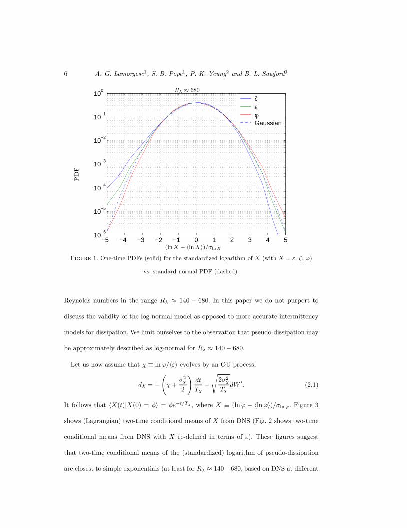
6 A. G. Lamorgese1, S. B. Pope1, P. K. Yeung2 and B. L. Sawford3
−5 −4 −3 −2 −1 0 1 2 3 4 510
−6
10−5
10−4
10−3
10−2
10−1
100
ζεφGaussian
Figure 1. One-time PDFs (solid) for the standardized logarithm of X (with X = ε, ζ, ϕ)
vs. standard normal PDF (dashed).
Rλ ≈ 680
PD
F
(lnX − 〈ln X〉)/σln X
Reynolds numbers in the range Rλ ≈ 140 − 680. In this paper we do not purport to
discuss the validity of the log-normal model as opposed to more accurate intermittency
models for dissipation. We limit ourselves to the observation that pseudo-dissipation may
be approximately described as log-normal for Rλ ≈ 140 − 680.
Let us now assume that χ ≡ lnϕ/〈ε〉 evolves by an OU process,
dχ = −(
χ +σ2
χ
2
)
dt
Tχ+
√
2σ2χ
TχdW ′. (2.1)
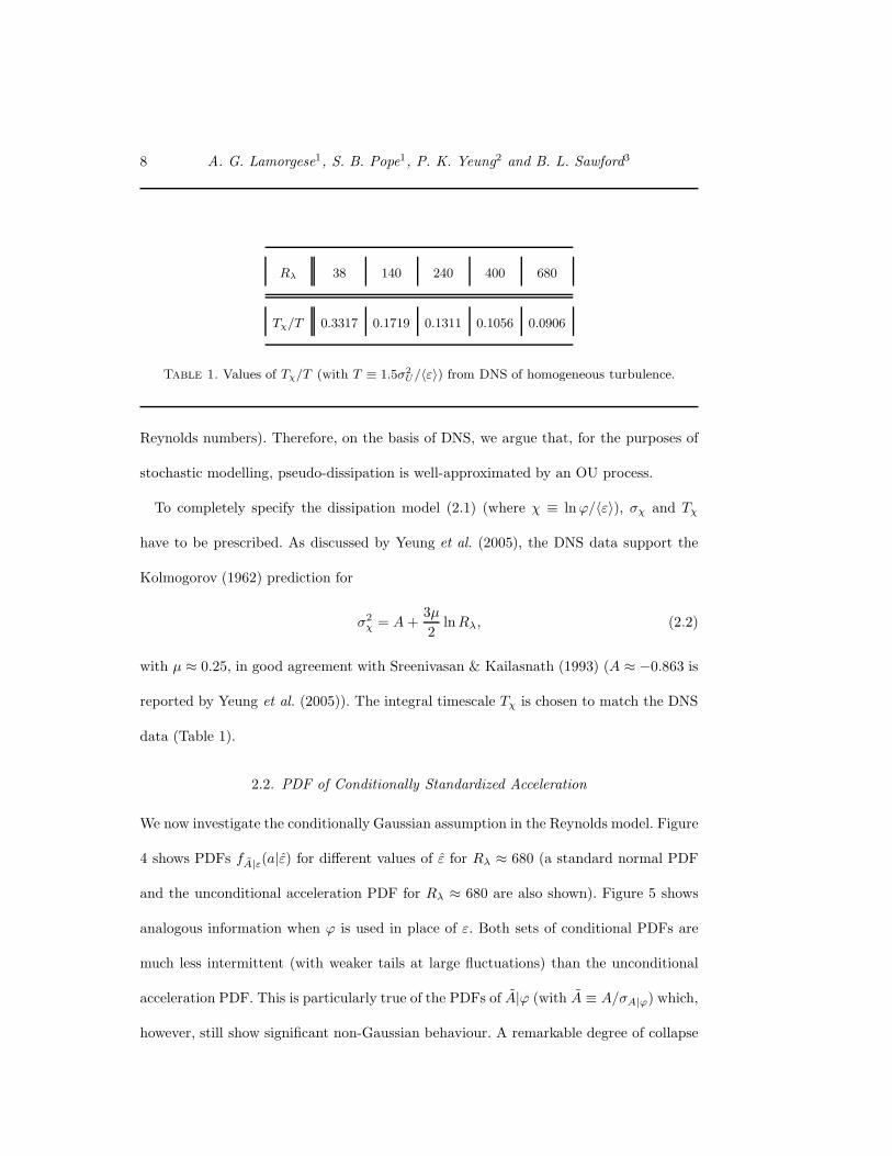
It follows that 〈X(t)|X(0) = φ〉 = φe−t/Tχ , where X ≡ (lnϕ − 〈lnϕ〉)/σln ϕ. Figure 3
shows (Lagrangian) two-time conditional means of X from DNS (Fig. 2 shows two-time
conditional means from DNS with X re-defined in terms of ε). These figures suggest
that two-time conditional means of the (standardized) logarithm of pseudo-dissipation
are closest to simple exponentials (at least for Rλ ≈ 140−680, based on DNS at different
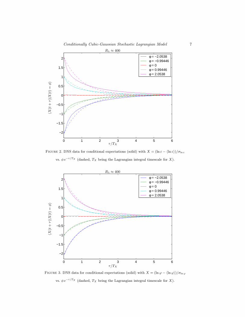
Conditionally Cubic-Gaussian Stochastic Lagrangian Model 7
0 1 2 3 4 5 6
−2
−1.5
−1
−0.5
0
0.5
1
1.5
2 φ = −2.0538 φ = −0.99446 φ = 0 φ = 0.99446 φ = 2.0538
Figure 2. DNS data for conditional expectations (solid) with X = (ln ε − 〈ln ε〉)/σln ε
vs. φ e−τ/TX (dashed, TX being the Lagrangian integral timescale for X).
Rλ ≈ 400〈X
(t+
τ)|X
(t)=
φ〉
τ/TX
0 1 2 3 4 5 6
−2
−1.5
−1
−0.5
0
0.5
1
1.5
2 φ = −2.0538 φ = −0.99446 φ = 0 φ = 0.99446 φ = 2.0538
Figure 3. DNS data for conditional expectations (solid) with X = (ln ϕ − 〈lnϕ〉)/σln ϕ
vs. φ e−τ/TX (dashed, TX being the Lagrangian integral timescale for X).
Rλ ≈ 400
〈X(t
+τ)|X
(t)=
φ〉
τ/TX
8 A. G. Lamorgese1, S. B. Pope1, P. K. Yeung2 and B. L. Sawford3
Rλ 38 140 240 400 680
Tχ/T 0.3317 0.1719 0.1311 0.1056 0.0906
Table 1. Values of Tχ/T (with T ≡ 1.5σ2
U/〈ε〉) from DNS of homogeneous turbulence.
Reynolds numbers). Therefore, on the basis of DNS, we argue that, for the purposes of
stochastic modelling, pseudo-dissipation is well-approximated by an OU process.
To completely specify the dissipation model (2.1) (where χ ≡ lnϕ/〈ε〉), σχ and Tχ
have to be prescribed. As discussed by Yeung et al. (2005), the DNS data support the
Kolmogorov (1962) prediction for
σ2
χ = A +3µ
2lnRλ, (2.2)
with µ ≈ 0.25, in good agreement with Sreenivasan & Kailasnath (1993) (A ≈ −0.863 is
reported by Yeung et al. (2005)). The integral timescale Tχ is chosen to match the DNS
data (Table 1).
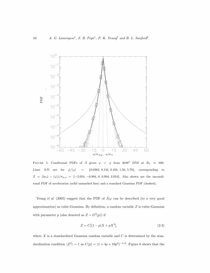
2.2. PDF of Conditionally Standardized Acceleration
We now investigate the conditionally Gaussian assumption in the Reynolds model. Figure
4 shows PDFs fA|ε(a|ε) for different values of ε for Rλ ≈ 680 (a standard normal PDF
and the unconditional acceleration PDF for Rλ ≈ 680 are also shown). Figure 5 shows
analogous information when ϕ is used in place of ε. Both sets of conditional PDFs are
much less intermittent (with weaker tails at large fluctuations) than the unconditional
acceleration PDF. This is particularly true of the PDFs of A|ϕ (with A ≡ A/σA|ϕ) which,
however, still show significant non-Gaussian behaviour. A remarkable degree of collapse
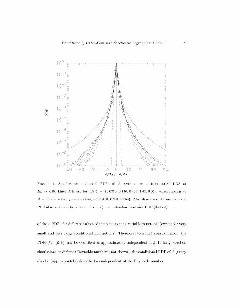
Conditionally Cubic-Gaussian Stochastic Lagrangian Model 9
|
Figure 4. Standardized onditional PDFs of A given ε = ε from 20483 DNS at
Rλ ≈ 680. Lines A-E are for ε/〈ε〉 = {0.0359, 0.136, 0.469, 1.62, 6.05}, corresponding to
Z = (ln ε − 〈ε〉)/σln ε = {−2.054, −0.994, 0, 0.994, 2.054}. Also shown are the unconditonal
PDF of acceleration (solid unmarked line) and a standard Gaussian PDF (dashed).
PD
F
a/σA|ε, a/σA
of these PDFs for different values of the conditioning variable is notable (except for very
small and very large conditional fluctuations). Therefore, to a first approximation, the
PDFs fA|ϕ(a|ϕ) may be described as approximately independent of ϕ. In fact, based on
simulations at different Reynolds numbers (not shown), the conditional PDF of A|ϕ may
also be (approximately) described as independent of the Reynolds number.
10 A. G. Lamorgese1, S. B. Pope1, P. K. Yeung2 and B. L. Sawford3
aa|ϕ
|
Figure 5. Conditional PDFs of A given ϕ = ϕ from 20483 DNS at Rλ ≈ 680.
Lines A-E are for ϕ/〈ϕ〉 = {0.0362, 0.134, 0.458, 1.56, 5.79}, corresponding to
Z = (ln ϕ − 〈ϕ〉)/σln ϕ = {−2.054, −0.994, 0, 0.994, 2.054}. Also shown are the uncondi-
tonal PDF of acceleration (solid unmarked line) and a standard Gaussian PDF (dashed).
PD
F
a/σA|ϕ, a/σA
Yeung et al. (2005) suggest that the PDF of A|ϕ can be described (to a very good
approximation) as cubic-Gaussian. By definition, a random variable Z is cubic-Gaussian
with parameter p (also denoted as Z ∼ G3(p)) if
Z = C[(1 − p)X + pX3], (2.3)
where X is a standardized Gaussian random variable and C is determined by the stan-
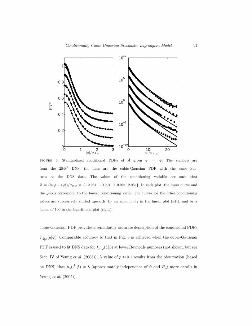
dardization condition 〈Z2〉 = 1 as C(p) = (1 + 4p + 10p2)−1/2. Figure 6 shows that the
Conditionally Cubic-Gaussian Stochastic Lagrangian Model 11
0 1 2 30
0.2
0.4
0.6
0.8
1
0 10 2010
−10
10−5
100
105
1010
Figure 6. Standardized conditional PDFs of A given ϕ = ϕ. The symbols are
from the 20483 DNS; the lines are the cubic-Gaussian PDF with the same kur-
tosis as the DNS data. The values of the conditioning variable are such that
Z = (ln ϕ − 〈ϕ〉)/σln ϕ = {−2.054, −0.994, 0, 0.994, 2.054}. In each plot, the lower curve and
the y-axis correspond to the lowest conditioning value. The curves for the other conditioning
values are successively shifted upwards, by an amount 0.2 in the linear plot (left), and by a
factor of 100 in the logarithmic plot (right).
PD
F
|a|/σA|ϕ |a|/σA|ϕ
cubic-Gaussian PDF provides a remarkably accurate description of the conditional PDFs
fA|ϕ(a|ϕ). Comparable accuracy to that in Fig. 6 is achieved when the cubic-Gaussian
PDF is used to fit DNS data for fA|ϕ(a|ϕ) at lower Reynolds numbers (not shown, but see
Sect. IV of Yeung et al. (2005)). A value of p ≈ 0.1 results from the observation (based
on DNS) that µ4(A|ϕ) ≈ 8 (approximately independent of ϕ and Rλ; more details in
Yeung et al. (2005)).
12 A. G. Lamorgese1, S. B. Pope1, P. K. Yeung2 and B. L. Sawford3
10−4
10−3
10−2
10−1
100
101
102
103
10−1
100
101
102
103
104
105
106
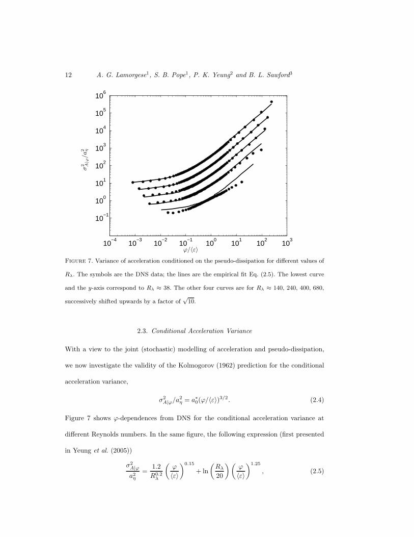
Figure 7. Variance of acceleration conditioned on the pseudo-dissipation for different values of
Rλ. The symbols are the DNS data; the lines are the empirical fit Eq. (2.5). The lowest curve
and the y-axis correspond to Rλ ≈ 38. The other four curves are for Rλ ≈ 140, 240, 400, 680,
successively shifted upwards by a factor of√
10.
σ2 A|ϕ
/a2 η
ϕ/〈ε〉
2.3. Conditional Acceleration Variance
With a view to the joint (stochastic) modelling of acceleration and pseudo-dissipation,
we now investigate the validity of the Kolmogorov (1962) prediction for the conditional
acceleration variance,
σ2
A|ϕ/a2
η = a∗0(ϕ/〈ε〉)3/2. (2.4)
Figure 7 shows ϕ-dependences from DNS for the conditional acceleration variance at
different Reynolds numbers. In the same figure, the following expression (first presented
in Yeung et al. (2005))
σ2
A|ϕ
a2η
=1.2
R0.2λ
(
ϕ
〈ε〉
)0.15
+ ln
(
Rλ
20
)(
ϕ
〈ε〉
)1.25
, (2.5)
Conditionally Cubic-Gaussian Stochastic Lagrangian Model 13
is shown to be an accurate representation (except at the smallest Rλ) of the DNS data.
As may be seen, the low-ϕ behaviour for the conditional acceleration variance deviates
strongly from that predicted by Eq. (2.4). Also, careful measurement of the slope for the
large-ϕ portion of the curves in Fig. 7 yields values that are systematically less than 1.5,
again at variance with the Kolmogorov (1962) prediction.
Equation (2.5) is most useful for stochastic modelling purposes because it accurately
parameterizes the conditional acceleration variance (given ϕ) in terms of both the value
being conditioned upon and the Reynolds number.
3. Conditionally Cubic-Gaussian (CCG) Stochastic Lagrangian
Models
Lagrangian statistics for ε, ζ and ϕ from DNS show that stochastic modelling is easiest
when pseudo-dissipation is used in place of the dissipation rate or the enstrophy. This
is because (i) ϕ is closest to log-normal, and (ii) two-time conditional means of lnϕ are
closest to exponential, and (iii) the conditional PDFs of acceleration given ϕ = ϕ collapse
best, and with the narrowest tails. Thus, we base the model on pseudo-dissipation ϕ and
take the OU process Eq. (2.1) as its stochastic model.
Conditioning on pseudo-dissipation is most useful when considering the joint-statistics
of acceleration and pseudo-dissipation because the PDF of A|ϕ may be described (to
a first approximation) as universal and, in particular, cubic-Gaussian. In other words,
given ϕ = ϕ and a standardized Gaussian random variable A, the acceleration A can be
modelled as
A = σA|ϕC[(1 − p)A + pA3]. (3.1)
For given ϕ, the relation between A and A is invertible (and one-to-one).
The stochastic model is most conveniently expressed in terms of the velocity U(t),
14 A. G. Lamorgese1, S. B. Pope1, P. K. Yeung2 and B. L. Sawford3
the “Gaussian” acceleration A(t) (related to the acceleration by Eq. (3.1)), and the log-
pseudo-dissipation variable χ∗ ≡ χ − 〈χ〉 = ln(ϕ/〈ε〉) − 〈ln(ϕ/〈ε〉)〉.
The model is
dU = Adt = σA|ϕC[(1 − p)A + pA3]dt, (3.2)
dA = θdt + bdW, (3.3)
dχ∗ = −χ∗ dt
Tχ+
√
2σ2χ
TχdW ′, (3.4)
where θ and b are drift and diffusion coefficients specified below.
The stationary one-time joint PDF of U, A and χ∗ is denoted by f(v, a, x∗), where v, a
and x∗ are sample-space variables corresponding to U, A and χ∗. We now assume that
this PDF is joint-normal with the variables being uncorrelated with each other (at the
same time). Thus, with the assumptions made the joint PDF is
f =1
σU
√2π
exp
(
− v2
2σ2
U
)
1√2π
exp
(
− a2
2
)
1
σχ
√2π
exp
(
− x∗2
2σ2χ
)
. (3.5)
The imposition of this PDF leads to a constraint for the drift coefficient θ in Eq. (3.3),
namely,
θ(v, a, ϕ) = −σA|ϕ
σ2
U
Cv(1 + p + pa2) +b2
2
∂
∂aln b2f + θ∗, (3.6)
where θ∗ is any function such that ∂∂a (θ∗f) = 0, which for simplicity we take to be zero.
We also introduce the assumption ∂b/∂a = 0 (which can be supported using an adiabatic
elimination argument in the limit Rλ → ∞). Then, Eq. (3.3) can be rewritten as
dA = − b2
2Adt − σA|ϕ
σ2
U
UC(1 + p + pA2)dt + bdW. (3.7)
This equation (together with Eqs. (3.2) and (3.4)) defines a class of CCG models,
i.e., different models with the same stationary distribution (3.5) correspond to differ-
ent choices of b. Each model captures the conditional dependence of acceleration on
pseudo-dissipation based on DNS (Eq. (2.5)) that accounts for deviations from the Kol-
Conditionally Cubic-Gaussian Stochastic Lagrangian Model 15
0 0.1 0.2 0.3 0.4 0.5 0.6 0.7 0.8 0.9
0
0.1
0.2
0.3
0.4
0.5
0.6
0.7
0.8
0.9
1c=0.7Re03u (DNS)v (DNS)w (DNS)
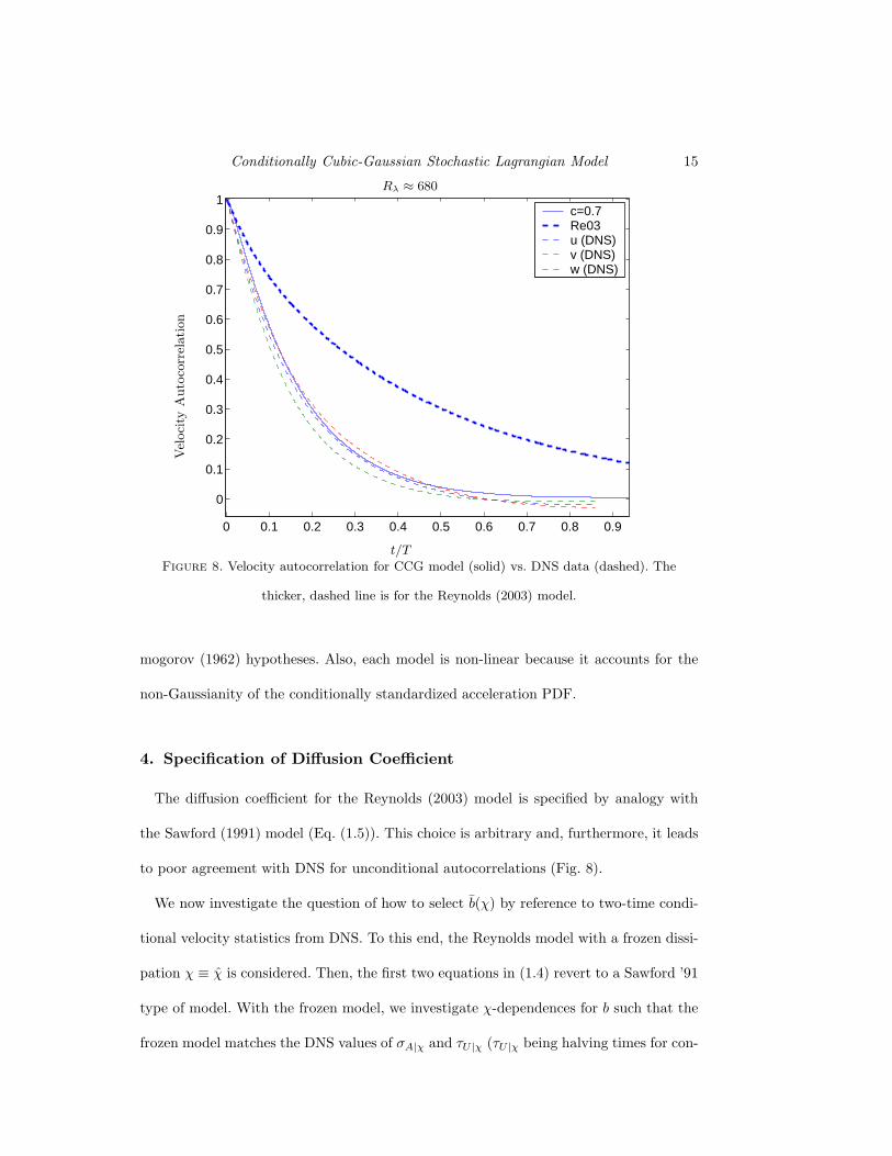
Figure 8. Velocity autocorrelation for CCG model (solid) vs. DNS data (dashed). The
thicker, dashed line is for the Reynolds (2003) model.
Rλ ≈ 680V
eloci
tyA
uto
corr
elation
t/T
mogorov (1962) hypotheses. Also, each model is non-linear because it accounts for the
non-Gaussianity of the conditionally standardized acceleration PDF.
4. Specification of Diffusion Coefficient
The diffusion coefficient for the Reynolds (2003) model is specified by analogy with
the Sawford (1991) model (Eq. (1.5)). This choice is arbitrary and, furthermore, it leads
to poor agreement with DNS for unconditional autocorrelations (Fig. 8).
We now investigate the question of how to select b(χ) by reference to two-time condi-
tional velocity statistics from DNS. To this end, the Reynolds model with a frozen dissi-
pation χ ≡ χ is considered. Then, the first two equations in (1.4) revert to a Sawford ’91
type of model. With the frozen model, we investigate χ-dependences for b such that the
frozen model matches the DNS values of σA|χ and τU|χ (τU|χ being halving times for con-
16 A. G. Lamorgese1, S. B. Pope1, P. K. Yeung2 and B. L. Sawford3
10−2
100
102
10−1
100
Rλ = 240
Rλ = 400
Rλ = 680
c=1
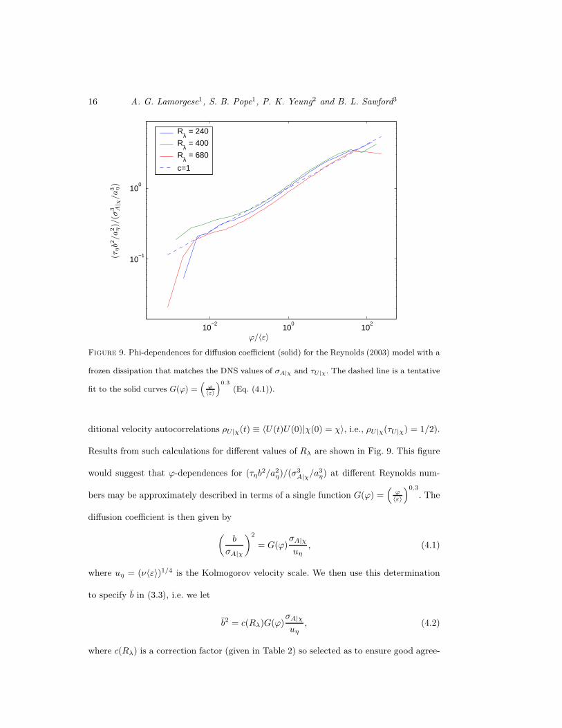
Figure 9. Phi-dependences for diffusion coefficient (solid) for the Reynolds (2003) model with a
frozen dissipation that matches the DNS values of σA|χ and τU|χ. The dashed line is a tentative
fit to the solid curves G(ϕ) =(
ϕ〈ε〉
)0.3
(Eq. (4.1)).
(τηb2
/a2 η)/
(σ3 A|χ
/a3 η)
ϕ/〈ε〉
ditional velocity autocorrelations ρU|χ(t) ≡ 〈U(t)U(0)|χ(0) = χ〉, i.e., ρU|χ(τU|χ) = 1/2).
Results from such calculations for different values of Rλ are shown in Fig. 9. This figure
would suggest that ϕ-dependences for (τηb2/a2η)/(σ3
A|χ/a3η) at different Reynolds num-
bers may be approximately described in terms of a single function G(ϕ) =(
ϕ〈ε〉
)0.3
. The
diffusion coefficient is then given by
(
b
σA|χ
)2
= G(ϕ)σA|χ
uη, (4.1)
where uη = (ν〈ε〉)1/4 is the Kolmogorov velocity scale. We then use this determination
to specify b in (3.3), i.e. we let
b2 = c(Rλ)G(ϕ)σA|χ
uη, (4.2)
where c(Rλ) is a correction factor (given in Table 2) so selected as to ensure good agree-
Conditionally Cubic-Gaussian Stochastic Lagrangian Model 17
0 0.2 0.4 0.6 0.8 1
0
0.2
0.4
0.6
0.8
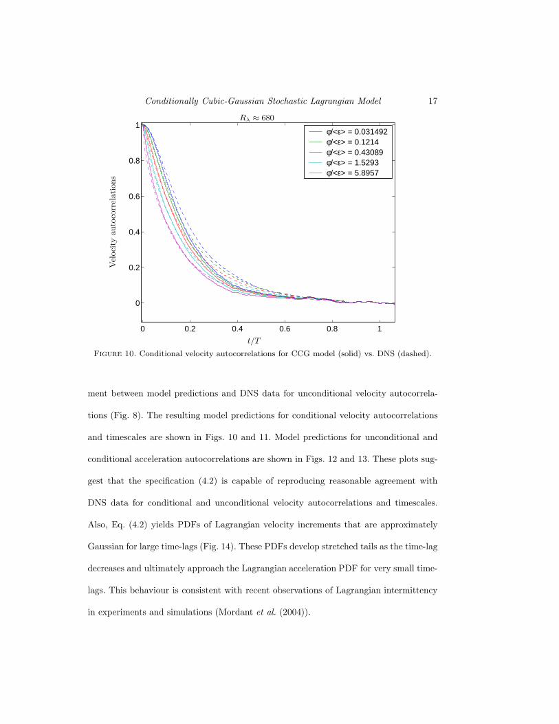
1φ/<ε> = 0.031492φ/<ε> = 0.1214φ/<ε> = 0.43089φ/<ε> = 1.5293φ/<ε> = 5.8957
Figure 10. Conditional velocity autocorrelations for CCG model (solid) vs. DNS (dashed).
Rλ ≈ 680V
eloci
tyauto
corr
elations
t/T
ment between model predictions and DNS data for unconditional velocity autocorrela-
tions (Fig. 8). The resulting model predictions for conditional velocity autocorrelations
and timescales are shown in Figs. 10 and 11. Model predictions for unconditional and
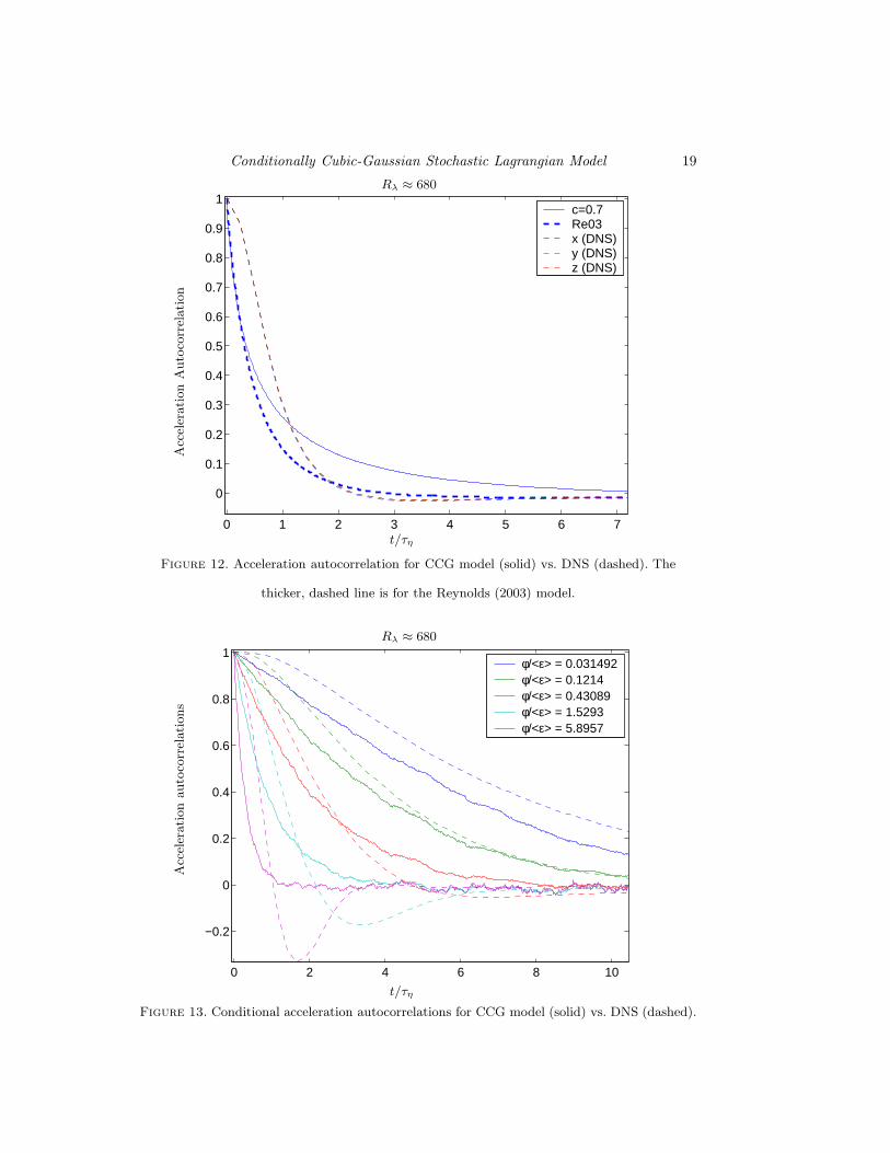
conditional acceleration autocorrelations are shown in Figs. 12 and 13. These plots sug-
gest that the specification (4.2) is capable of reproducing reasonable agreement with
DNS data for conditional and unconditional velocity autocorrelations and timescales.
Also, Eq. (4.2) yields PDFs of Lagrangian velocity increments that are approximately
Gaussian for large time-lags (Fig. 14). These PDFs develop stretched tails as the time-lag
decreases and ultimately approach the Lagrangian acceleration PDF for very small time-
lags. This behaviour is consistent with recent observations of Lagrangian intermittency
in experiments and simulations (Mordant et al. (2004)).
18 A. G. Lamorgese1, S. B. Pope1, P. K. Yeung2 and B. L. Sawford3
10−2
10−1
100
101
102
10−1
(4.2)
DNS
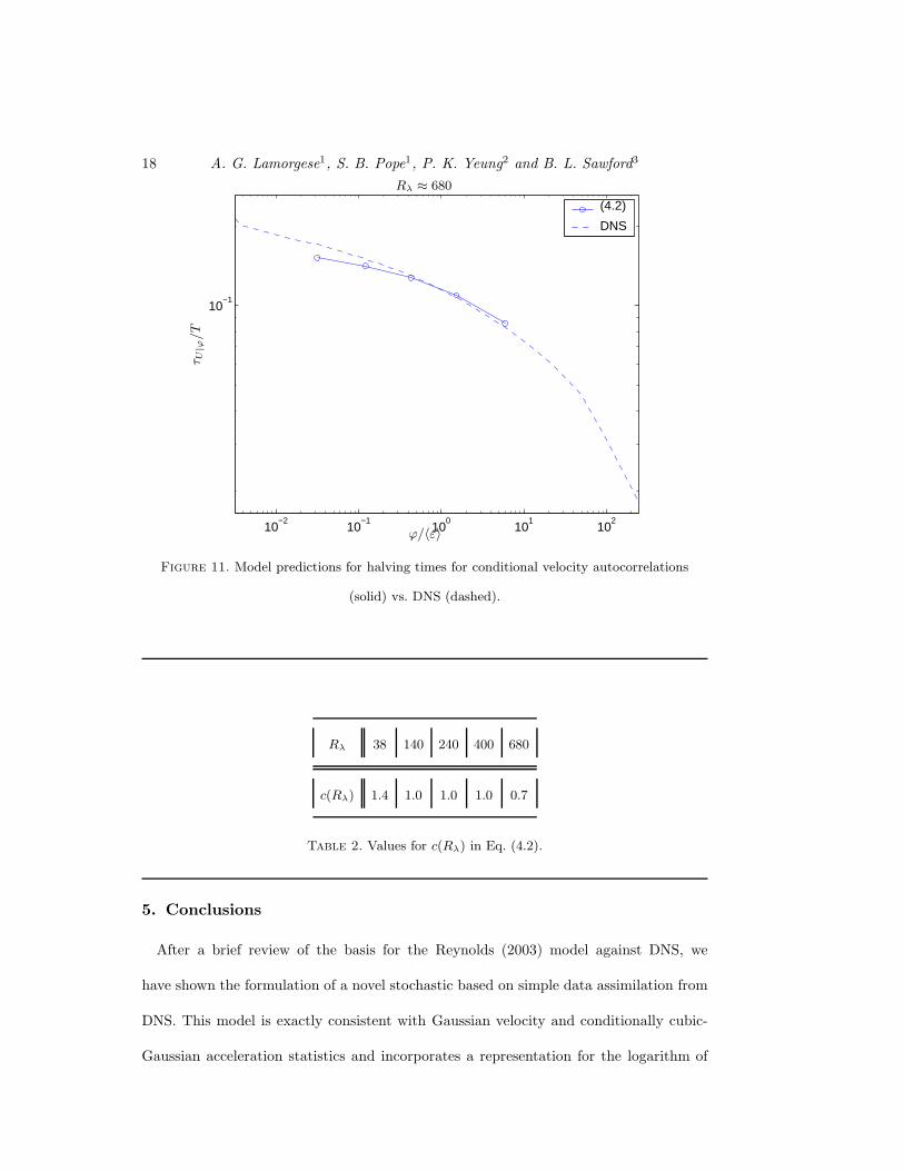
Figure 11. Model predictions for halving times for conditional velocity autocorrelations
(solid) vs. DNS (dashed).
Rλ ≈ 680τ U
|ϕ/T
ϕ/〈ε〉
Rλ 38 140 240 400 680
c(Rλ) 1.4 1.0 1.0 1.0 0.7
Table 2. Values for c(Rλ) in Eq. (4.2).
5. Conclusions
After a brief review of the basis for the Reynolds (2003) model against DNS, we
have shown the formulation of a novel stochastic based on simple data assimilation from
DNS. This model is exactly consistent with Gaussian velocity and conditionally cubic-
Gaussian acceleration statistics and incorporates a representation for the logarithm of
Conditionally Cubic-Gaussian Stochastic Lagrangian Model 19
0 1 2 3 4 5 6 7
0
0.1
0.2
0.3
0.4
0.5
0.6
0.7
0.8
0.9
1c=0.7Re03x (DNS)y (DNS)z (DNS)
Figure 12. Acceleration autocorrelation for CCG model (solid) vs. DNS (dashed). The
thicker, dashed line is for the Reynolds (2003) model.
Rλ ≈ 680A
ccel
eration
Auto
corr
elation
t/τη
0 2 4 6 8 10
−0.2
0
0.2
0.4
0.6
0.8
1φ/<ε> = 0.031492φ/<ε> = 0.1214φ/<ε> = 0.43089φ/<ε> = 1.5293φ/<ε> = 5.8957
Figure 13. Conditional acceleration autocorrelations for CCG model (solid) vs. DNS (dashed).
Rλ ≈ 680
Acc
eler
ation
auto
corr
elations
t/τη
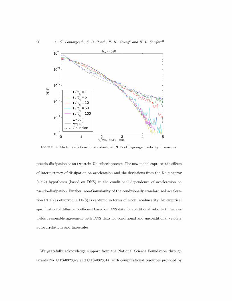
20 A. G. Lamorgese1, S. B. Pope1, P. K. Yeung2 and B. L. Sawford3
0 1 2 3 4 510
−5
10−4
10−3
10−2
10−1
100
τ / τη = 1
τ / τη = 5
τ / τη = 10
τ / τη = 50
τ / τη = 100
U−pdfA−pdfGaussian
Figure 14. Model predictions for standardized PDFs of Lagrangian velocity increments.
Rλ ≈ 680P
DF
v/σU , a/σA, etc.
pseudo-dissipation as an Ornstein-Uhlenbeck process. The new model captures the effects
of intermittency of dissipation on acceleration and the deviations from the Kolmogorov
(1962) hypotheses (based on DNS) in the conditional dependence of acceleration on
pseudo-dissipation. Further, non-Gaussianity of the conditionally standardized accelera-
tion PDF (as observed in DNS) is captured in terms of model nonlinearity. An empirical
specification of diffusion coefficient based on DNS data for conditional velocity timescales
yields reasonable agreement with DNS data for conditional and unconditional velocity
autocorrelations and timescales.
We gratefully acknowledge support from the National Science Foundation through
Grants No. CTS-0328329 and CTS-0328314, with computational resources provided by
Conditionally Cubic-Gaussian Stochastic Lagrangian Model 21
the Pittsburgh Supercomputing Center and the San Diego Supercomputer Center, which
are both supported by NSF.
REFERENCES
Beck, C. 2001 Dynamical foundations of nonextensive statistical mechanics. Physical Review
Letters 87 (18), 180601.
Beck, C. 2002 Lagrangian acceleration statistics in turbulent flows. Europhysics Letters 64 (2),
151 – 7.
Biferale, L., Boffetta, G., Celani, A., Lanotte, A. & Toschi, F. 2005 Particle trapping
in three-dimensional fully developed turbulence. Physics of Fluids 17 (2), 021701.
Christensen, K. T. & Adrian, R. J. 2002 Measurement of instantaneous Eulerian acceleration
fields by particle image accelerometry: Method and accuracy. Experiments in Fluids 33 (6),
759 – 769.
Gylfason, A., Ayyalasomayajula, S. & Warhaft, Z. 2004 Intermittency, pressure and
acceleration statistics from hot-wire measurements in wind-tunnel turbulence. Journal of
Fluid Mechanics 501, 213 – 229.
La Porta, A., Voth, G. A., Crawford, A. M., Alexander, J. & Bodenschatz, E. 2001
Fluid particle accelerations in fully developed turbulence. Nature 409, 1017 – 19.
Mordant, N., Leveque, E. & Pinton, J.-F. 2004 Experimental and numerical study of the
Lagrangian dynamics of high Reynolds number turbulence. New Journal of Physics 6,
116–159.
Pope, S. B. 2002 A stochastic Lagrangian model for acceleration in turbulent flows. Physics of
Fluids 14 (7), 2360 – 75.
Pope, S. B. & Chen, Y. L. 1990 The velocity-dissipation probability density function model
for turbulent flows. Physics of Fluids A 2 (8), 1437 – 49.
Reynolds, A. M. 2003 On the application of nonextensive statistics to Lagrangian turbulence.
Physics of Fluids 15 (1), L1.
Sawford, B. L. 1991 Reynolds number effects in Lagrangian stochastic models of turbulent
dispersion. Physics of Fluids A 3 (6), 1577 – 86.
22 A. G. Lamorgese1, S. B. Pope1, P. K. Yeung2 and B. L. Sawford3
Sreenivasan, K. R. & Kailasnath, P. 1993 Update on the intermittency exponent in turbu-
lence. Physics of Fluids A 5 (2), 512.
Vedula, P. & Yeung, P. K. 1999 Similarity scaling of acceleration and pressure statistics in
numerical simulations of isotropic turbulence. Physics of Fluids 11 (5), 1208.
Voth, G. A., La Porta, A., Crawford, A. M., Alexander, J. & Bodenschatz, E. 2002
Measurement of particle accelerations in fully developed turbulence. Journal of Fluid Me-
chanics 469, 121 – 160.
Voth, G. A., Satyanarayan, K. & Bodenschatz, E. 1998 Lagrangian acceleration measure-
ments at large Reynolds numbers. Physics of Fluids 10 (9), 2268 – 80.
Yeung, P. K. 1997 One- and two-particle Lagrangian acceleration correlations in numerically
simulated homogeneous turbulence. Physics of Fluids 9 (10), 2981.
Yeung, P. K. & Pope, S. B. 1989 Lagrangian statistics from direct numerical simulations of
isotropic turbulence. Journal of Fluid Mechanics 207, 531 – 586.
Yeung, P. K., Pope, S. B., Lamorgese, A. G. & Donzis, D. A. 2005 Acceleration and
dissipation statistics in numerical simulations of isotropic turbulence (submitted to Physics
of Fluids).
Related Documents