
Welcome message from author
This document is posted to help you gain knowledge. Please leave a comment to let me know what you think about it! Share it to your friends and learn new things together.
Transcript

K Ai
A Concrete Approach to Abstract Algebra

A Concrete Approach
to Abstract
Algebra
W. W. Sawyer
W. H. Freeman and Company
SAN FRANCISCO, 1959

The writing of this book, which was prepared while the
author was teaching at the University of Illinois, as a
member of the Academic Year Institute, 1957-1958, was
supported in part by a grant from the National Science
Foundation.
© Copyright 1959 by W. H. Freeman and Company, Inc. All
rights to reproduce this book in whole or in part are reserved,
with the exception of the right to use short quotations for review
of the book. Printed in the United States of America. Library of
Congress Catalogue Card Number: 59-10215

Contents
Introduction 1
1 The Viewpoint of Abstract Algebra 5
2 Arithmetics and Polynomials 26
3 Finite Arithmetics 71
4 An Analogy Between Integers and Polynomials 83
5 An Application of the Analogy 94
6 Extending Fields 115
7 Linear Dependence and Vector Spaces 131
8 Algebraic Calculations with Vectors 157
9 Vectors Over a Field 167
10 Fields Regarded as Vector Spaces 185
1 1 Trisection of an Angle 208
Answers to Exercises 223

Introduction
The Aim of This Book
and How to Read It
At the present time there is a widespread desire,
particularly among high school teachers and engineers,
to know more about “modern mathematics.” Institutes
are provided to meet this desire, and this book wasoriginally written for, and used by, such an institute.
The chapters of this book were handed out as mimeo-graphed notes to the students. There were no “lectures”;
I did not in the classroom try to expound the same mate-rial again. These chapters were the “lectures.” In the
classroom we simply argued about this material. Ques-tions were asked, obscure points were clarified.
In planning such a course, a professor must make a
choice. His aim may be to produce a perfect mathemat-ical work of art, having every axiom stated, every con-
clusion drawn with flawless logic, the whole syllabus
covered. This sounds excellent, but in practice the result
is often that the class does not have the faintest idea of
what is going on. Certain axioms are stated. How are
these axioms chosen? Why do we consider these axiomsrather than others? What is the subject about? What is
its purpose? If these questions are left unanswered, stu-
dents feel frustrated. Even though they follow every

2 A Concrete Approach to Abstract Algebra
individual deduction, they cannot think effectively about
the subject. The framework is lacking; students do not
know where the subject fits in, and this has a paralyzing
effect on the mind.
On the other hand, the professor may choose familiar
topics as a starting point. The students collect material,
work problems, observe regularities, frame hypotheses,
discover and prove theorems for themselves. The work
may not proceed so quickly;
all topics may not be
covered; the final outline may be jagged. But the student
knows what he is doing and where he is going; he is
secure in his mastery of the subject, strengthened in con-
fidence of himself. He has had the experience of discover-
ing mathematics. He no longer thinks of mathematics
as static dogma learned by rote. He sees mathematics
as something growing and developing, mathematical
concepts as something continually revised and enriched
in the light of new knowledge. The course may have cov-
ered a very limited region, but it should leave the student
ready to explore further on his own.
This second approach, proceeding from the familiar
to the unfamiliar, is the method used in this book.
Wherever possible, I have tried to show how modern
higher algebra grows out of traditional elementary alge-
bra. Even so, you may for a time experience some feeling
of strangeness. This sense of strangeness will pass; there
is nothing you can do about it; we all experience such
feelings whenever we begin a new branch of mathemat-
ics. Nor is it surprising that such strangeness should be
felt. The traditional high school syllabus—algebra, ge-
ometry, trigonometry—contains little or nothing dis-
covered since the year 1650 a.d. Even if we bring in
calculus and differential equations, the date 1750 a.d.
covers most of that. Modern higher algebra was de-
veloped round about the years 1900 to 1930 a.d. Anyone

Introduction 3
who tries to learn modern algebra on the basis of tradi-
tional algebra faces some of the difficulties that Rip VanWinkle would have experienced, had his awakening
been delayed until the twentieth century. Rip wouldonly overcome that sense of strangeness by riding around
in airplanes until he was quite blase about the whole
business.
.. Some comments on the plan of the book may be
helpful. Chapter 1 is introductory and will not, I hope,
prove difficult reading. Chapter 2 is rather a long one.
In a book for professional mathematicians, the whole
content of this chapter would fill only a few lines. I
tried to spell out in detail just what those few lines wouldconvey to a mathematician. Chapter 2 was the result.
The chapter contains a solid block of rather formal
calculations (pages 50-56). Psychologically, it seemed a
pity to have such a block early in the book, but logically
I did not see where else I could put it. I would advise
you not to take these calculations too seriously at a first
reading. The ideas are explained before the calculations
begin. The calculations are there simply to show that
the program can be carried through. At a first reading,
you may like to take my word for this and skip pages
50-56. Later, when you have seen the trend of the whole
book, you may return to these formal proofs. I would
particularly emphasize that the later chapters do not in
any way depend on the details of these calculations
—
only on the results.
The middle of the book is fairly plain sailing. Youshould be able to read these chapters fairly easily.
I am indebted to Professor Joseph Landin of the
University of Illinois for the suggestion that the book
should culminate with the proof that angles cannot be
trisected by Euclidean means. This proof, in chapter 11,
shows how modern algebraic concepts can be used to

4 A Concrete Approach to Abstract Algebra
solve an ancient problem. This proof is a goal toward
which the earlier chapters work.
I assume, if you are a reader of this book, that you
are reasonably familiar with elementary algebra. Oneimportant result of elementary algebra seems not to be
widely known. This is the remainder theorem. It states
that when a polynomial f(x) is divided by x — a, the
remainder is f(a). If you are not familiar with this
theorem and its simple proof, it would be wise to review
these, with the help of a text in traditional algebra.

Chapter i
The Viewpoint of Abstract
Algebra
There are two ways in which children do arithmetic
—by understanding and by rote. A good teacher, cer-
tainly in the earlier stages, aims at getting children to
understand what 5—2 and 6X8 mean. Later, he
may drill them so that they will answer “48” to the
question “Eight sixes?” without having to draw eight
sets of six dots and count them.
Suppose a foreign child enters the class. This child
knows no arithmetic, and no English, but has a most
retentive memory. He listens to what goes on. He notices
that some questions are different from others. For in-
stance, when the teacher makes the noise “What day is
it today?” the children may make the noise “Monday”or “Tuesday” or “Wednesday” or “Thursday” or “Fri-
day.” This question, he notices, has five different an-
swers. There are also questions with two possible answers,
“Yes” and “No.” For example, to the question “Haveyou finished this sum?” sometimes one, sometimes the
other answer is given.
However, there are questions that always receive the
same answer. “Hi” receives the answer “Hi.” “Twelve

6 A Concrete Approa ch to Abstract Algebra
twelves?” receives the answer “A hundred and forty-
four”—or, at least, the teacher seems more satisfied
when this response is given. Soon the foreign child might
learn to make these responses, without realizing that
“Hi” and “144” are in rather different categories.
Suppose that the foreign child comes to school after
the children in his class have finished working with blocks
and beads. He sees 12 X 12 = 144 written and hears it
spoken, but is never present when 12 is related to the
counting of twelve objects.
One cannot say that he understands arithmetic, but
he may be top of the class when it comes to reciting the
multiplication table. With an excellent memory, he mayhave complete mastery of formal, mechanical arithmetic.
We may thus separate two elements in arithmetic,
(i) The formal element—this covers everything the for-
eign child can observe and learn. Formal arithmetic is
arithmetic seen from the outside, (ii) The intuitive ele-
ment—the understanding of arithmetic, its meaning,
its connection with the actual world. This understand-
ing we derive by being part of the actual universe, by
experiencing life and seeing it from the inside.
For teaching, both elements of arithmetic are neces-
sary. But there are certain activities for which the formal
approach is helpful. In the formalist philosophy of math-
ematics, a kind of behaviorist view is taken. Instead of
asking “How do mathematicians think?” the formalist
philosophers ask “What do mathematicians do?” Theylook at mathematics from the outside: they see mathe-
maticians writing on paper, and they seek rules or laws
to describe how the mathematicians behave.
Formalist philosophy is hardly likely to provide a full
picture of mathematics, but it does illuminate certain
aspects of mathematics.
A practical application of formalism is the design of
all kinds of calculating machines and automatic appli-
T he Viewpoint of Abstract Algebra 7
ances. A calculating machine is not expected to under-
stand what 71 X 493 means, but it is expected to give
the right answer. A fire alarm is not expected to under-
stand the danger to life and the damage to property
involved in a fire. It is expected to ring bells, to turn onsprinklers, and so forth. There may even be some con-
nection between the way these mechanisms operate andthe behavior of certain parts of the brain.
One might say that the abstract approach studies
what a machine is, without bothering about what it
is for.
Naturally, you may feel it is a waste of time to study
a mechanism that has no purpose. But the abstract ap-
proach does not imply that a system has no meaningand no use; it merely implies that, for the moment, weare studying the structure of the system, rather than its
purpose.
Structure and purpose are in fact two ways of classify-
ing things. In comparing a car and an airplane, youwould say that the propeller of an airplane corresponds
to the driving wheels of a car if you are thinking in terms
of purpose; you would however say that the propeller
corresponds to the cooling fan if you are thinking in
terms of structure.
Needless to say, a person familiar with all kinds of
mechanical structures—wheels, levers, pulleys, and so
on—can make use of that knowledge in inventing amechanism. In a really original invention, a structure
might be put to a purpose it had never served before.
Arithmetic Regarded as a Structure
Accordingly, we are going to look at arithmetic fromthe viewpoint of the foreign student. We shall forget
that 12 is a number used for counting, and that + andX have definite meanings. We shall see these things

8 A Concrete Approach to Abstract Algebra
purely as signs written on the keys of a machine.
Stimulus: 12 X 12.
Response: 144.
Our calculating machine would have the following
visible parts:
(i) A space where the first number is recorded.
(ii) A space for the operations +, X, —
,
(iii) A space for the second number.
These constitute the input.
The output is the answer, a single number.
Playing around with our machine, we would soon
observe certain things. Order is important with -r- and— . Thus 6 -T- 2 gives the answer 3, while 2 -r- 6 gives
the answer 1/3. But order is not important with + and
X • Thus 3 + 4 and 4 + 3 both give 7 ; 3 X 4 and 4X3both give 12.
We have the commutative laws: a b = £ + a, a X. b =b X a. (Or ab = ba, with the usual convention of leav-
ing out the multiplication sign.)
Commutativity is not something that could have been
predicted in advance. Since 6 -S- 2 is not the same as
2 "7" 6, we could not say, for any sign S, that
a S b — b S a.
Some comment may be made here on the symbol S.
In school algebra, letters usually stand for numbers. In
what we are doing, letters stand for things written on the
keys of machines. The form a S b covers, for example,
a “times” b,
a “plus” b,
a “minus” b,
a “over” b,
a “to the power” b,
a “-th root of” b,
a “-’s log to base” b,

The Viewpoint of Abstract Algebra 9
as well as many more complicated ways of combining
a and b that one could devise.
Commutativity, then, is something we may notice
about a machine. It is one example of the kind of
remark that can be made about a machine.
Ordinary arithmetic has one property that is incon-
venient for machine purposes: it is infinite. If we makea calculating machine that goes up to 999,999 weare unable to work out, say, 999,999 + 999,999 or
999,999 X 999,999 by following the ordinary rules for
operating the machine.
We can consider a particular calculating machine that
is very much simpler, and that avoids the trouble of
infinity. This machine will answer any question appropri-
ate to its system. It deals with a particular part or aspect
of arithmetic.
If two even numbers are added together, the result is
an even number. If an even number is added to an odd
number, the result is odd. We may, in fact, write
Even -f- Even = Even
Even + Odd = OddOdd + Odd = Even.
Similarly, there are multiplication facts,
Even X Even = Even
Even X Odd = Even
Odd X Odd = Odd.
Here we have a miniature arithmetic. There are only
two elements in it, Even and Odd. Let us abbreviate,
writing A for Even, B for Odd. Then
A A = A A XA = AA + B = B AX B = AB + A = B B X A = AB + B = A B X B = B

10 A Concrete Approach to Abstract Algebra
which may be written more compactly as
A B
,a Fa b
+ B B A
A
1A
B~A
B
Our foreign student would have no reason for regard-
ing A and B in the tables above as any different from
0, 1, 2, 3,• •
•,in the ordinary addition and multiplica-
tion tables. He might think of it as “another arithmetic.”
He does not know anything about its meaning. Whatcan he observe about its structure? Does it behave at all
like ordinary arithmetic? In actual fact, the similarities
are very great. I shall only mention a few of them at
this stage.
Both addition and multiplication are commutative in
the A, B arithmetic. For instance, A + B = B + A and
A X B = B X A.
In ordinary arithmetic the number zero occurs. Weknow the meaning of zero. But how could zero be iden-
tified by someone who only saw the structure of arith-
metic? Quite easily, for there are two properties of zero
that single it out. First, when zero is added to a number,
it makes no difference. Second, whatever number zero
is multiplied by, the result is always zero.
Thus
x + 0 = x,
x • 0 = 0.
Is there a symbol in the A, B arithmetic that plays
the role of zero? It makes a difference when B is added
:
A + B is not A, nor is B + B the same as B. A is the
only possible candidate, and in fact A passes all the tests.
When you add A, it makes no difference; when anything
is multiplied by A, you get A.
Is there anything that corresponds to 1? The only dis-

The Viewpoint of Abstract Algebra 11
tinguishing property I can think of for 1 is that mul-tiplication by 1 has no visible effect:
*•1 = x.
In the A, B arithmetic, multiplication by B leavesany symbol unchanged. So B plays the part of 1.
This suggests that we might have done better tochoose O (capital o) as a symbol instead of A and I as
a symbol instead of B, because O looks like zero, and I
looks rather like 1
.
Our tables would then read
0 + 0 = 00 + 1=11+0 = 1
1 + 1=0
0X0 = 00X1=01X0 = 0I X I = I
Now this looks very much like ordinary arithmetic.In fact, the only question that would be raised by some-body who thought I stood for 1 and O for zero would be,
“Haven’t you made a mistake in writing I + I = O?”All the other statements are exactly what you wouldexpect from ordinary arithmetic.
The tables of this “arithmetic” are
+ 01
O I
0 I
1 o
O I
o oO I
We arrived at the tables above by considering evenand odd numbers. But we could arrive at the same pat-tern without any mention of numbers.
Imagine the following situation. There is a narrowbridge with automatic signals. If a car approaches fromeither end, a signal “All clear—Proceed” is flashed on.But if cars approach from both ends, a warning signal

12 A Concrete Approach to Abstract Algebra
is flashed, and the car at, say, the north end is instructed
to withdraw.
In effect, the mechanism asks two questions: “Is a car
approaching from the south? Is one approaching fromthe north?” The answers to these questions are the input,
the stimulus. The output, the response of the mechanism,is to switch on an appropriate signal.
For the all-clear signal the scheme is as follows.
Should all-clear signal be flashed?
Car from north?
No Yes
Car Nofromsouth? Yes
For the warning signal the scheme is as follows.
Should warning signal be flashed?
Car from north?
No Yes
Car Nofromsouth? Yes
If you compare these tables with the earlier ones, youwill see that they are exactly the same in structure.
“No” replaces “O,” “Yes” replaces “I”; “all clear” is
related to +, “warning signal” to X.One could also realize this pattern by simple electrical
circuits.
O O 0 0
.1
0

The Viewpoint of Abstract Algebra 13
If you had this machine in front of you, you would not
know whether it was intended for calculations with even
and odd numbers, or for traffic control, or for some other
purpose.
When the same pattern is embodied in two different
systems, the systems are called isomorphic. In our exam-
ple above, the traffic control system is isomorphic with
the arithmetic of Even and Odd. The same machine
does for both.
Isomorphism does not simply mean that there is some
general resemblance between the two systems. It means
that they have exactly the same pattern. Our example
above shows this exact correspondence. Wherever “O”occurs in one system, “No” occurs in the other; wher-
ever “I” occurs in one system, “Yes” occurs in the other.
The statements, “these two systems are isomorphic”
and “there is an isomorphism between them,” are two
different ways of saying the same thing. To prove two
systems isomorphic, you must demonstrate a correspond-
ence between them, like the one in our example.
The study of structures has two things to offer us.
First, the same structure may have many different re-
alizations. By studying the single structure, we are simul-
taneously learning several different subjects.
Second, even though we have only one realization of
our structure in mind, we may be able to simplify our
proofs and clarify our understanding of the subject by
treating it abstractly—that is to say, by leaving out
details that merely complicate the picture and are not
relevant to our purpose.
Our Results Considered Abstractly
So far we have been concrete in our approach. That is,
we have been talking of things whose meaning we under-

14 A Concrete Approach to Abstract Algebra
stand—numbers, Even and Odd, Yes and No. This is,
of course, desirable from a teaching point of view, to
avoid an unbearable sense of strangeness.
Now let us look at what we have found purely in terms
of pattern, of structure, and without reference to any
particular interpretation or application it may have.
That is, we return strictly to the point of view of the
foreign student. What can we say?
Well, first of all, we can recognize what belongs to
the subject. Arithmetic deals with 0, 1,2, 3, 4, 5, 6, 7,
8, 9. 7 is an element of arithmetic; “Hi” is not. “O”and “I” were elements used in our miniature arithmetic.
“Yes” and “No” were elements in the traffic problem.
The various positions of the switches were elements in
the electrical mechanism.
So, first of all, our subject deals with a certain set of
recognizable objects. Then we have a certain procedure
with these objects. If we take the electrical machine
marked +, and set the first switch to I, the second to O,
the machine gives us the response I. We say I + O is I.
In the same way, if the teacher asks “3 + 4?” the chil-
dren respond “7.”
We may call adding and multiplying operations. Amachine might be devised to do many other operations
besides.
Thus in arithmetic we specify the objects 3, 4 andthe operation “add” (+). The machine or the class
gives us another object, 7, as a response.
We can list the things we noted earlier about arith-
metic.
(1) Arithmetic deals with a certain set of objects.
(2) Given any two of these objects a, b, another object
called their sum is uniquely defined. If c is the sumof a and b, we write c = a + b.

The Viewpoint of Abstract Algebra 15
(3) In the same way a product k is defined. We write
k = a X b or k = a- b.
(4) a + b and b + a are the same object.
(5) a-b and b-a are the same object.
(6) There is an object 0 such that a + 0 = a and<3-0 = 0 for every a.
(7) There is an object 1 such that a • 1 = a for every a.
These are not all the things that could be said about
arithmetic. We have not mentioned the associative laws,
{a + b) + c = a + {b + c), a-(b-c) = (a-b)-c; the dis-
tributive law, a(x +jy) = ax -f- ay; nor anything about
subtraction and division.
However, suppose we agree that statements (1)
through (7) are enough to think about for the moment.We might ask, “Is ordinary arithmetic the only struc-
ture with these properties? If not, what is the smallest
number of objects with which this structure can be
realized?”
We already have the answer to both questions. Arith-
metic is not the only structure satisfying statements (1)
through (7). The smallest structure consists of the ob-
jects O, I with the tables for + and X given earlier.
(We are assuming that 0 and 1 are distinct objects.)
EXERCISES
1. Let O stand for “any number divisible by 3,” I for “anynumber of the form 3n + 1,” and II for “any number of the
form 3n + 2.” Can one say to what class a + b will belong
if one knows to what classes a and b belong? And the product ab?
If so, form tables of addition and multiplication, as we did
with the tables for Even and Odd. Do statements (1) through
(7) apply to this topic?
16, A Concrete Approach to Abstract Algebra
2. The same as question 1, but with the classes O, I, II, III,
IV for numbers of the forms 5n, 5« + 1, 5n + 2, 5n + 3,
5n + 4.
3. Continue the inquiry for other numbers, 4, 6, 7,• •
•,
replacing 3 and 5 of questions 1 and 2. Do you notice any
differences between the results for different numbers?
4. An arithmetic is formed as follows. The only permitted
objects are 0, 2, 4, 6, 8. When two numbers are added or
multiplied, only the last digit is recorded. For example, in
ordinary arithmetic 6 + 8 = 14 with last digit 4. In this arith-
metic 6 + 8 = 4. Normally 4 X 8 = 32 with last digit 2. So
here 4X8 = 2. Write out the addition and multiplication
tables. Do statements (1) through (7) apply here? This arith-
metic contains five objects, as did the arithmetic of question 2.
Are the arithmetics isomorphic?
5. Calculate the powers of II, of III, and of IV in the
arithmetic of question 2.
6. Are subtraction and division possible in the arithmetic of
question 2? Do they have unique answers? What about the
arithmetics you studied under question 3?
7. In the arithmetic of question 2, which numbers are per-
fect squares? Which numbers are prime? Does this arithmetic
have any need of (i) negative numbers, (ii) fractions?
Two Arithmetics Compared
There is a certain stage in the learning of arithmetic
at which the only operations known are addition, sub-
traction, multiplication, and division. The child has not
yet met V2, but is familiar with whole numbers and
fractions. I am not sure whether it would be so in cur-
rent educational practice, but we shall suppose the child
knows about negative numbers.
The charm of this stage of knowledge is that every
question has an answer. You must not, of course, ask for
division by zero, but, apart from this reasonable restric-
The Viewpoint of Abstract Algebra 17
tion, if you are given any two numbers you can add,
subtract, multiply, or divide and reach a definite answer.
The body of numbers known to a child at this stage
are referred to as the rational numbers. The rational
numbers comprise all numbers of the form p/q, where
p and q are whole numbers (positive or negative); p can
also be zero but q must not. Since q can be 1, we havenot excluded the whole numbers themselves.
The operations the child knows at this stage we maycall the rational operations. A rational operation is any-
thing that can be done by means of addition, subtrac-
tion, multiplication, and division, each used as often as
you like. For instance,
(* + D(y - h)
X
is the result of a rational operation on x and y. Note,
however, that the process must finish. A child in grade
school is not expected to cope with an expression like
1 +2 +
2 +2 +
2 +and so on forever. This expression, in a certain sense,
represents V2. The study of unending processes belongs to
analysis: we exclude any such idea from algebra.
To sum up: There is a stage when a child sees arith-
metic as consisting of rational operations on rational
numbers. At this stage, every question has an answer,
every calculation can be carried out.
Now we consider another arithmetic. On an island in
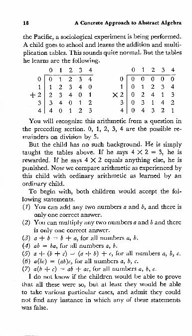
18 A Concrete Approach to Abstract Algebra
the Pacific, a sociological experiment is being performed.
A child goes to school and learns the addition and multi-
plication tables. This sounds quite normal. But the tables
he learns are the following.
0
1
+ 2
3
4
0 12 3 4
0 12 3 4
1 2 3 4 0
2 3 4 0 1
3 4 0 1 2
4 0 12 3
0
1
X 2
3
4
0 12 3 4
0 0 0 0 0
0 12 3 4
0 2 4 1 3
0 3 14 2
0 4 3 2 1
You will recognize this arithmetic from a question in
the preceding section. 0, 1, 2, 3, 4 are the possible re-
mainders on division by 5.
But the child has no such background. He is simply
taught the tables above. If he says 4 X 2 = 3, he is
rewarded. If he says 4X2 equals anything else, he is
punished. Now we compare arithmetic as experienced by
this child with ordinary arithmetic as learned by an
ordinary child.
To begin with, both children would accept the fol-
lowing statements.
(/) You can add any two numbers a and b, and there is
only one correct answer.
(2) You can multiply any two numbers a and b and there
is only one correct answer.
(3) a + b — b + a, for all numbers a,
b.
(
4
) ab = ba,for all numbers a, b.
(5) a + (b + c) = (a + b) + c, for all numbers a, b, c.
(6) a(bc) =(ab)c ,
for all numbers a, b, c.
(7) a(b + c) = ab + ac, for all numbers a, b, c.
I do not know if the children would be able to prove
that all these were so, but at least they would be able
to take various particular cases, and admit they could
not find any instance in which any of these statements
was false.
The Viewpoint of Abstract Algebra 19
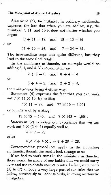
Statement (5), for instance, in ordinary arithmetic,
expresses the fact that when you are adding, say, the
numbers 7, 11, and 13 it does not matter whether youargue
7 + 11 = 18, and 18 + 13 = 31
or
11 + 13 = 24, and 7 + 24 = 31.
The intermediate steps look quite different, but they
lead to the same final result.
In the miniature arithmetic, an example would beadding 2, 3, and 4. You could either say
2 + 3 = 0, and 0 + 4 = 4or
3 + 4 = 2, and 2 + 2=4,the final answer being 4 either way.
Statement (6) expresses the fact that you can workout 7 X 11 X 13, by writing
7X11= 77, and 77 X 13 = 1,001
or equally well by writing
11 X 13 = 143, and 7 X 143 = 1,001.
Statement (7) expresses our experience that we canwork out 4 X (2 + 5) equally well as
4
X 7 = 28
or as
4X2 + 4X5 = 8 + 20 = 28.
Corresponding procedures apply in the miniature
arithmetic, though the results look strange to us.
If we had to work sums in the miniature arithmetic,
there would be many of our habits that we could carry
over and use to obtain correct results. In fact, statements
(3) to (7) embody a very large part of the rules that wefollow, consciously or unconsciously, in doing arithmetic
or algebra.

20 A Concrete Approach to Abstract Algebra
Subtraction and Division
Our seven statements above make no mention of sub-
traction or division. When we learn arithmetic, 7 — 4
is probably explained as “4 and what are 7?” This is,
in everything except language, an invitation to solve the
equation 4 + * = 7. Further, grade school teachers have
a strong prejudice to the effect that this equation has
only one solution, x — 3.
The formal statement (8
)
below therefore contains
nothing more than our own infant experiences.
(8) (i) For all a and b, the equation a + x = b has a
solution, (ii) The equation has only one solution,
(iii) This solution is called b — a.
Here (i) and (ii) make statements that can be tested bytaking particular numbers for a and b. Statement (iii)
merely explains what we understand by the new sym-
bol, —,that we have just brought in. It does not require
testing or proof. It shows us, however, how to find, say,
2 — 3 in the miniature arithmetic. 2 — 3 is the numberthat satisfies 3 + x — 2. In the addition table, we mustlook along the row opposite 3, until we find the num-ber 2. We find it under 4, and only under 4. 3 -j- 4 = 2,
and no other number will do in place of 4. So 2 — 3 = 4
is correct, and is the only correct answer.
Question: What does the requirement, that a + x = b
shall have one and only one solution for all a and b, tell us
about the rows of the addition table?
When you subtract a number from itself, the answer
is zero. We might express this in the statement: a — a
has a fixed value, independent of what a is; this value
is called 0.
As a — a = 0 means the same thing as a = a + 0, wecan equally well put this statement in the following
form (that we have already met).

The Viewpoint of Abstract Algebra 21
(9) There is a number 0 such that, for every a, a + 0 = a.
There can of course only be one such number; other-
wise a x = a would have more than one solution,
which would contradict part (ii) of statement (8).
Now we come to division. As children we meet divi-
sion in much the same way as subtraction. “4 and what
is 12?” is replaced by “4 times what is 12?” We might
begin to write a statement, on the lines of (8), that
ax — b has a solution, and only one solution, whatever
a and b. But this would overlook the fact that
0 -* = 0
is satisfied by every number x, so that this equation has
more than one solution, while
0-x = 1
is not satisfied by any number x.
Apart from this point, there is no difficulty in giving
a formal statement of our experiences with division.
(10) For all a and b, provided however that a is not 0,
(i) ax = b has a solution, (ii) This equation has
only one solution, (iii) The solution is called
b -§- a or b/a.
Just as we can find a — a to be 0 without knowing
what number a is, we know in ordinary arithmetic that
a -f a or a/a is 1, without needing to know what a is,
except of course that a is not 0.
So, as statement (8) was followed by (9), statement
(10) is followed by (11).
(11) There is a number 1 such that, for every a, a • 1 = a.
If you will now test statements (8), (9), (10), (11) for
the miniature arithmetic, you will find that all of them
work for it too.
This is quite remarkable. Within the set 0, 1, 2, 3, 4,
without having to introduce any fresh numbers (like
negative numbers or fractions in ordinary arithmetic),

22 A Concrete Approach to Abstract Algebra
we can add, subtract, multiply, and divide to our heart’s
content.
For instance, in the miniature arithmetic, simplify
(1 + fHt-l)3 3.
UT 4
We can get rid of the fractions in the numerator anddenominator immediately:
| = 1 V 2 = 3,
f = 2 -h 3 = 4,
f = 3 -f- 4 = 2,
f = 3 -5- 2 = 4.
The fraction is simplified to
(3 + 4). (4 -2) _ 2-2 _4-2 2
There are many different ways in which this expres-
sion could be simplified. In the denominator, for in-
stance, we could say 3/2 — 3/4 = 3/4; and then divi-
sion by 3/4 is the same as multiplication by 4/3. This
would give
i • (i + 1) • (t - !),
which can still be simplified in several ways. But how-ever we proceed, we shall always arrive at the answer 2.
You may have noticed that 2 — 3 = 4, 3-1-2 = 4.
This shows that, for x = 2, x — 3 = 3/x. Are there anyother solutions of this equation? We have
x
Multiply by x:
x2 — 3x = 3.
Subtract 3. Since 0 — 3 = 2, this gives
x2 — 3x + 2 = 0.
(* — l)(x — 2) = 0.

The Viewpoint of Abstract Algebra 23
So x — 1 and * = 2 are solutions. Could there be anymore solutions? To show there are not we need to ob-
serve (72).
(72) ab = 0 only if a = 0 or b = 0. In words, a product
is zero only if a factor is zero.
Above we had (x — 1)(* — 2) = 0. Either
* — 1= 0 or * — 2 = 0;
* = 1 or * = 2.
Thus quadratics can be solved by factoring exactly as
in ordinary arithmetic. They can also be solved bycompleting the square. For example, consider
*2 + x = 2.
To complete the square for *2 + ax, we add {a/2) 2 to
each side. In our equation a = 1, so a/2 = 3, since
2X3 = 1. We must add to each side 32,that is, 4. Thus
*2 + * + 32 = 2 + 4 = 1,
(* + 3)2 = 1.
Next we have to take the square root. I2 = 1 and also
42 = 1. (Note that 4 = 0 — 1, so that ±1 is the sameas 1 or 4.) Thus
* + 3 = 1 or * + 3 = 4;
* = 3 or * = 1.
One can test by substituting these values in the orig-
inal equation that they actually are roots.
This arithmetic will be referred to as “the arithmetic
modulo 5.” The number 5 in this title indicates that weare dealing with 0, 1, 2, 3, 4, the possible remainders
on division by 5.
In the same way, the arithmetic of Even and Odd,with elements 0, 1 is called “arithmetic modulo 2.”
(On division by 2, an even number leaves remainder 0,
an odd number 1.)

24 A Concrete Approach to Abstract Algebra
In earlier exercises, you were invited to study the
arithmetics modulo 3, modulo 4, modulo 6, modulo 7,
and so on.
EXERCISES
1. Make a table of squares, cubes, and fourth powers
modulo 5. Solve the equations x2 = 1, x3 = 1, x* = 1 in this
arithmetic.
2. Find (x + y)5 modulo 5.
3. Divide x2 + 1 by x -f- 2, modulo 5. Has x2 + 1 =0any solutions in this arithmetic? What are they?
4. In the text we solved x2 + x = 2, modulo 5. This equa-
tion may be written x2 + x + 3 = 0. What are the factors of
x2 + x + 3?
5. Find by trial, by completing the square, or by any
other method, the solutions of the following equations in the
arithmetic modulo 5:(i) x2 + 2x + 2 = 0, (ii) x2 + 3x + 1 =0,
(iii) x2 + x -j- 4 = 0, (iv) x2 + 4 = 0. What are the factors of
the quadratic expressions that occur in the equations above?
6. Divide Xs + 2x2 + 3x + 4 by x — 2 in the arithmetic
modulo 5.
7. Does the remainder theorem hold in the arithmetic
modulo 5?
8. Does the equation (x — 3)2 = 0 have any solution other
than x — 3 in the arithmetic modulo 4?
9. In the arithmetic modulo 6 calculate the values of
x2 + 3x + 2 for x = 0, 1, 2, 3, 4, 5. How many roots does the
quadratic equation x2 + 3x + 2 = 0 have in this arithmetic?
10. All the statements (7) through (72) are true in the
arithmetic modulo 5. Which of them hold in (i) the arithmetic
modulo 4, (ii) the arithmetic modulo 6?
11. Can it be proved that a quadratic equation has at most
two roots (i) in an arithmetic where statements (7) through (9)

The Viewpoint of Abstract Algebra 25
and (77) only are known to hold? (ii) in an arithmetic where
statements (7) through (72) are known to hold?
12. In the arithmetic modulo 5 are there any quadratics
*2 + px + q (i) that have no solutions when equated to zero?
(ii) that cannot be split into factors of the form (x + «)(* + b)?
13. In the arithmetic modulo 5 the equation x3 = 2 has the
solution 3. Has it any other solutions? Divide x3 — 2 by x — 3.
Has the resulting quadratic any factors?

Chapter 2
Arithmetics and Polynomials
We have now met three kinds of arithmetic. Our or-
dinary arithmetic is the first kind. It deals with numbers
0, 1, 2,• •
•,that go on forever.
The arithmetic modulo 5 is the second kind. It con-
tains only 0, 1, 2, 3, 4, but in spite of this it is remarkably
like ordinary arithmetic. I can still ask you quite con-
ventional questions in algebra—to multiply expressions,
to do long division, to solve a quadratic, to factor a
polynomial, to prove the remainder theorem.
The third type is shown by arithmetic modulo 4 or
modulo 6. It diverges still further from ordinary arith-
metic. A quadratic may have more than two roots;
still more striking, division ceases to be possible. In
modulo 6 arithmetic, 3-r 2 has no answer, while 4 + 2
has the answers 2 and 5. However, some similarities to
ordinary arithmetic remain. We can still multiply with-
out restriction. We can divide by 1 and 5, and this means
that we can divide by x — a or 5x — a. The remainder
theorem, that a polynomial f(x) on division by x — a
leaves the remainder /(a), still makes sense and is true.
It will be helpful in considering these arithmetics, and
other structures that we shall meet, to tabulate their
properties. On the left side of our table, we write our

Rational
Natural
Statements
numbers
numbers
Integers
Modulo
5
Modulo
6
27
+ + + + + + + C1 + o + +
S3
+
+
+S3
^ S3
V3 -S3
rt)
S3 g
+-r-S3
^3X!<Ua
<43 XS<U <u
X5 fl
** *S M + 53
+?+!+'
(U
.S''3
3
~S XS3 44 c/3
oo
-S3 •S3-S3 -S3
x to<u .53
X „ Xflj <3 CJ
S3 S3 S3 S3 S3 S3 S3 -S3 O -S3

28 A Concrete Approach to Abstract Algebra
statements (7) through (72). Across the top of the table,
we write the names of the structures we plan to “test.”
If a structure satisfies the tests, or statements, we enter
a plus sign in the proper column. If a structure fails to
satisfy a test, or statement, we enter a zero. It is often
the property that is lacking that gives a peculiar flavor.
Across the top of our table we have the following struc-
tures listed: (i) The rational numbers; (ii) The natural
numbers 0, 1, 2,• •
•;
(iii) The integers 0, ±1, ±2, •;
(iv) The arithmetic modulo 5 ;(v) The arithmetic mod-
ulo 6.
In future, we shall define various types of structures by
saying which tests are passed. A table of this kind gives
a convenient way of recording definitions and of classify-
ing any particular structure.
We shall give one such definition straight away. Our
table shows two structures that make exactly the same
score—the rational numbers and the arithmetic mod-
ulo 5. Now we have had several examples to show that
you can work modulo 5 very much as you do in ordinary
arithmetic. We therefore introduce a name to express
this kind of similarity.
definition. Any structure that passes all the tests (7)
through (12) is called a field.
It is hard to hold all the twelve tests in mind at once,
and a rather looser explanation may be easier to remem-
ber. A field is a structure in which you can add, subtract,
multiply, and divide, and these operations behave very
much as they do in elementary arithmetic. Tests (7)
through (72) make precise what I mean by “behave
very much alike.”
It may be well to collect together the twelve tests,
and to state them in a way that we can use generally.
Several of them were stated above in terms of the child
in the Pacific Island.

Arithmetics and Polynomials 29
Every structure we consider contains elements. We are
not concerned with what these elements are; they maybe marks on paper, sounds of words, physical objects,
parts of a calculating machine, thoughts in the mind.
We also have operations +, X or +, . These opera-
tions need not have any connection with addition andmultiplication in arithmetic, other than the purely for-
mal resemblance required by the tests below. We think
again of our calculating machine, with two spaces for
elements a, b; one space for a sign + or •
;and a space
for the answer. We understand by a + b or a-b whatappears in the answer space—regardless of the internal
mechanism of the calculating machine.
The following twelve statements will henceforth be
referred to as the axioms for a field.
(7)
To any two elements a, b and the operation +, there
corresponds a uniquely defined element c. We write
c = a + b.
(2) To any two elements a, b and the operation there
corresponds a uniquely defined element d. We write
d = a-b.
(3) a + b = b + a, for all elements a ,b.
(4) a-b = b-a,for all elements a, b.
(5) a + (b + c) = (a + b) + c, for all elements a, b, c.
(6) a-(b-c) =(a-b)-c , for all elements a, b, c.
(7) a-(b + c) = (a-b) -j- (a-c), for all elements a, b, c.
(8) For any elements a and b, we can find one and only one
element x such that a + x = b. We call this element
b — a.
(9) There is a unique element 0 such that a + 0 = a for
every element a.
(10) For any elements a and b, provided only that a is not 0,
there is one and only one element x such that ax = b.
We call this element b/a.

30 A Concrete Approa ch to Abstract Algebra
(11) There is a unique element 1 such that for every a, a - 1 = a.
The element 1 is not the same as the element 0.
(12) a-b = 0 only if a = 0 or b = 0.
(Students sometimes ask, “Ought we not include as
an axiom that <2-0 = 0 for all a?” This, however, can
be proved from the axioms we already have. By axioms (9)
and (11), 1 +0 = 1. Therefore, a- (1 + 0) = a- 1. By ax-
iom (7), a- 1 + a- 0 = a- 1. By axiom (11), a + a-0 = a.
This says that x = a- 0 satisfies the equation a + x = a.
Axiom (8) shows that this equation has only one solu-
tion. Axiom (9) states that this solution is * = 0. So
a- 0 = 0. Note that axiom (12) is intended to be read
in this sense: “If you know that ab is zero, you can deduce
that either a is zero or b is zero.” The result we have
just proved is the converse of this.)
In all of these axioms it should be understood that by
“element” we mean an element in the structure. For
instance, suppose we are applying the tests to the nat-
ural numbers 0, 1, 2, 3,• • • . Someone might say, “Test
(10) is passed, because if you take any quotient like
3 4 it does exist; it is 3/4.” But 3/4 is not an element
in the set 0, 1, 2, 3,• • • . It is true that by bringing in new
elements 1/2, 3/4, -1, -2, and so on, you can obtain a
field, the field of rational numbers in which division and
subtraction are always possible. When we say that a
structure is a field, we mean that it already contains
the answers to every subtraction and division question.
A child that only knows the numbers 0, 1, 2, 3,• •
•,can
only answer the questions “Take 4 from 3,” “Divide 3
by 4” by saying “You can’t take 4 from 3,” “4 doesn’t
go into 3.” This indicates that the natural numbers do
not form a field; they fail tests (5) and (10).
I have not attempted to reduce the tests to the smallest
possible number, as might be done in a study of axiomat-
ics. For instance, it is quite easy to show that a structure

Arithmetics and Polynomials 31
that passes tests (7) through (77) also passes (72). Someof my tests could be cut down somewhat; part could be
assumed and the remainder proved. My purpose at
present is to explain what a field is, and to give a speedy
way of recognizing one.
EXERCISES
Determine which of the following are fields, and show on the
chart which tests each passes. (At this stage you may find it
best to convince yourself that certain properties do or do not
apply, without necessarily being able to provide formal proof.)
1 . The even numbers, 0, 2, 4, 6,• • • .
2. The even numbers, including negative numbers, 0, ±2,±4, • • • .
3. The real numbers.
4. The complex numbers, x + iy, where x, y are real.
5. The complex numbers, p -f- iq, where p, q are rational.
6. The complex numbers, m + in, where m, n are integers.
7. All numbers of the form p + qy/2, where p, q are ra-
tional.
8. All expressions a + bx, where a, b are real numbers.
9. All polynomials in x with real coefficients.
10. All functions P(x)/Q{x), where P(x) and Q(x) are poly-
nomials with real coefficients.
1 1 . Arithmetic modulo 2.
12. Arithmetic modulo 3.
13. Arithmetic modulo 4.
Question for Investigation
If n is a positive whole number, what condition must
n satisfy if the arithmetic modulo n is to be a field? It is

32 A Concrete Approach to Abstract Algebra
fairly easy to find out experimentally what the condition
is. It is also easy to show that the condition is necessary;
that is, that arithmetic modulo n cannot be a field unless
n has a certain property. It is harder to prove that this
property is sufficient to ensure the arithmetic being a
field.
A field is so much like our ordinary arithmetic that wecan work with its elements just as if they were ordinary
numbers;our usual habits lead us to correct results, and
we feel quite at home.
But some structures, as we have seen, are provided
with operations that we can label + and •,but yet fall
short of being fields. One or more of statements (7)
through (72) proves false.
There are still other structures in which we do not
have two operations, but only one. For example, wemight consider the structure in which every element
was of the form “x dogs and y cats,” x and y of course
being positive whole numbers, or zero. It would be nat-
ural to have the operation + defined to correspond to the
word “and.”
If a is 3 dogs and 4 cats,
b is 5 dogs and 6 cats,
a + b is 8 dogs and 10 cats.
But there is no obvious way of defining the operation •
;
we can hardly say that dog times dog is a square dog.
We shall later meet less frivolous examples in which
only one operation, either + or • occurs.
These are, of course, simpler structures than arith-
metic, and logically it would be reasonable to start
with them and work up to arithmetic and other struc-
tures with two operations. However, it seemed wiser to
start with the familiar subject of arithmetic, and only at

Arithmetics and Polynomials 33
this stage to indicate that it occupies a fairly lofty posi-
tion in the family of all possible structures.
One might go beyond arithmetic to study structures
with three operations, +, •, and * say. Whether any-
thing of mathematical interest or value would be found
in this way, I do not know.
Polynomials Over Any Field
The examples in chapter 1 suggested very strongly
that most of the properties of polynomials in ordinary
algebra were also true when we were working with the
arithmetic modulo 5. It should be possible to generalize
from this, and to find properties true for any field F—that is to say, for any system obeying axioms (7) through
(72).
When we write the quadratic ax2-f- bx + c, we may
have in mind, for example,
(i) a,b, c integers,
(ii) a, b, c rational numbers,
(iii) a, b, c real numbers,
(iv) a, b, c complex numbers,
(v) a, b, c 0 or 1 in the arithmetic modulo 2,
(vi) a, b, c 0,1, 2, 3, or 4 in the arithmetic modulo 5.
In case (i) we say that ax2 + bx + c is a quadratic
polynomial over the integers. Thus llx2 — Ax + 3 is a
polynomial over the integers.
In case (ii) we speak of a polynomial over the field of
rational numbers; for example, \x2 — fx +In case (iii) we have a polynomial over the field of
real numbers; for example x2 + -kx — e.
In case (iv) we have a polynomial over the field of
complex numbers; for example, (1 + i)x2 + (J — 0* +(3 + 4f).

34 A Concrete Approach to Abstract Algebra
In case (v) we have a quadratic over the arithmetic
modulo 2; for example lx2 + Oat + 1.
In case (vi) we have a quadratic over the arithmetic
modulo 5; say, 2x 2—f— 3x -f- 1 . This does not look any
different from a quadratic over the integers. Perhaps if
we write (2x2 + 3x + 1) = 2(x -J- l)(x + 3), the dis-
tinction will become apparent. You could, if you like, use
a symbolism we had earlier, and write Hat2-f- III* + I,
where the Roman numerals emphasize that we are
dealing with numbers modulo 5.
The word “over” has always seemed to me a little
queer in this connection. Perhaps it is used because the
coefficients can range over the elements of the field F.
Anyway, all that matters is its meaning. axn + bxn~ x
+ • •• 4- kx + m is a polynomial over the field F, if a
,
b, • • • m are all elements of F. The idea is a simple
one.
The Scope of x
The step we have just taken corresponds to the begin-
ning of school algebra, a, b, ••
•,k, m are numbers of the
arithmetic (see examples (i) through (vi) of the previous
subheading). The symbol a is something new. We have
passed from 11, —4, 3 to llx 2 — 4x + 3.
The best pupils are not deceived by the apparent
newness. They say, “You can test whether a statement
about x is true by seeing whether it holds for any num-
ber.” The worst pupils do not look at it this way. They
have no idea what x means, but they manage to pick up
certain rules for working with x.
Curiously enough, both points of view are significant
for modern algebra. They lead to an important distinc-
tion. There are certain expressions (in certain fields F)
that are equal when x is replaced by any number of the

Arithmetics and Polynomials 35
field, but they are not equal in the sense of being the
same expression. The best pupils will say they are equal;
the worst pupils will say they are not.
An example will make this clear. Suppose our field Fconsists of the numbers 0, 1 of arithmetic modulo 2. If
we ask a dull pupil “Is x2 -\- x equal to 0?” the pupil will
say “No.” We ask, “Why?” The pupil answers, “Well,
they are different, x2 + x is x2 + x, and 0 is 0. They are
two different things.”
If we ask a bright pupil, who thinks of algebra as gen-
eralized arithmetic, “Is x2 + x equal to 0 in the arith-
metic modplo 2?” this pupil will answer, “Let me see.
If * was 0, x2 -\- x would be 0. If x was 1, x2 + x would
be 1 + 1) which is 0. 0 and 1 are the only numbers in
the field F. Yes; x2 + x is always the same number as 0.”
Actually, we have to regard both answers as correct.
They are in effect answers to two different questions;
they correspond to two different interpretations of equal.
We shall need both of these ideas, and some agreed wayof expressing them.
If /(x) and g(x) are two algebraic expressions which,
when simplified in accordance with the rules of an
algebra, lead to one and the same polynomial ax" +bxn
~ l 4- • •• 4~ kx 4" m, we say that /(x) and g(x) are
formally equal.
If in /(x) and g(x), when we replace the symbol x by
any element of the field F, the resulting values are the
same, we say /(x) equals ^(x) for every x in the field F.
Thus, for modulo 2 arithmetic, x 2 4" * and 0 are not
formally equal, but they are equal for every x in the field.
In ordinary algebra, it is not necessary to make this
distinction. There is a well-known theorem that if /(x)
and g(x) are two polynomials equal for all rational num-bers (or even for all integers), then /(x) and g{x) are
formally equal.

36 A Concrete Approach to Abstract Algebra
In a field with a finite number of elements, this dis-
tinction is bound to arise. For instance, arithmetic
modulo 3 contains only the numbers 0, 1, 2. Evidently
x(x — l)(x — 2) is zero for x = 0, for x = 1, and for
x = 2. So x(x — l)(x — 2) = 0 for every x in the field.
But if you multiply this expression out, you get an answer
which is not Ox 3 -j- Ox 2 + Ox -f- 0. So x(x — l)(x — 2) is
not formally equal to zero.
Question: Multiply out x(x — l)(x — 2) modulo 3.
Find and multiply out the corresponding expression for
the arithmetic modulo 5.
The fact just noted can be important. For instance,
the equation x2 = 2 has no solution in the field F con-
sisting of 0, 1, 2 modulo 3. We might want to bring in
a new sign, \^2, and extend our arithmetic just as we dowith ordinary numbers. Now x(x — l)(x — 2) is not zero
for x = \^2. If we are going to extend our numbersystem in this way, it is the dull child’s answer and not
the bright one’s that is helpful
!
There are in fact three roles that x can play: (i) It maystand for any element of the field F. (ii) It may stand for
certain elements outside the field F. (iii) It may not stand
for anything at all—it may be just a mark on a calculat-
ing machine.
Ordinary high school algebra is a sufficient example
of (i), where it is understood that any statement about
x holds for every number of arithmetic.
As an example of (ii) we might consider, say, %x 2 —-Jx — 5. This is a polynomial over the rationals. But we
can consider the result of putting x = V/2orx = 7rin
this expression. Neither number is rational.
A more striking example can be found from calculus.
(This is simply an example. Any student unfamiliar
with calculus can omit it, as it is not needed for later

Arithmetics and Polynomials 37
developments.) Let f(t) stand for any function of t that
is capable of being differentiated as often as we wish. Let
D stand for the operation d/dt so that
W) = /'(*)
DJ(t) = f"(t)
D 3f(t) = and so on.
By an expression such as (D 2 +2D 3)/(?), we shall
understand /"(0 + 2/'(0 -j- 3f{t). (This example is in-
tended to convey what we understand by addition of the
operations D 2,2D, and 3.)
Multiplication of operations means that the operations
are to be applied successively. Thus, if I want to apply
{D + 2) • (D 3) to f(t), I begin by finding (.D 4" 3)f{t).
Let this be u(t). I then apply the operation (D + 2) to
u(t), and get (D -j- 2)u(t), that is, u!{t) + 2u(t), whereu(t) = (£)-}- 3)f(t) = f{t) -fi 3ft). If I substitute this
value of u(t) in u'{t) + 2u(t) I get
/"(0 + 3f(t) + 2fit) + 6/(0 = f’{t) + 5fit) + 6/(0.
To summarize what we have done: Applying the op-
eration D 4- 3 to ft) gives f{t) 4- 3ft). Applying the
operation D 4- 2 to the result above gives f'{t) 4~ 5/'(0
4~ 6/(0« This last expression is what we understand by(D 4~ 2) • (D 4~ 3) acting on/(0-
But the result above could be written (
D
2 4~ 3D 4“ 6)
ft). That is: the operation (D 4~ 2) • (D 4~ 3) applied
to any function has the same effect as D2 4“ 3D 4- 6
applied to the same function. We naturally call these
two operations equal. In symbols
(D 4- 2)-(D 4- 3) = D 2 4- 5D f 6.
But this result has a familiar look. It is exactly whatwe should get if we forgot all about D standing for d/dt
and simply applied the rules of elementary algebra.
Thus, in certain circumstances, we are entitled to*

38 A Concrete Approach to Abstract Algebra
substitute in x 2 + 5x + 6 the value x = d/dt,which is
not a number at all. This fact is made use of in teaching
engineering students how to solve certain types of differ-
ential equations.
Finally, we may—as we did toward the end of the
last example—say “let us forget all about the meaning
of x, and simply remember than x may be manipulated
according to certain rules.” This is the fully abstract
approach. It corresponds to possibility (iii) above.
The kind of theorem that can be obtained by the ab-
stract approach is shown by the following important
result. If you have a calculating machine with certain
signs marked on it (the numbers or elements of F) and
also two operations, + and •,for which the twelve
field axioms hold, then you can build a calculating
machine that will have all those signs and also the signs
x, x2,x 3
,
• • • . On this enlarged machine, addition and
multiplication will still be possible; the commutative,
associative, and distributive laws will still hold.
In other words, if you have any field F, and you in-
troduce a new symbol x without inquiring at all into the
meaning of x, and you perform calculations with poly-
nomials in x (the coefficients being elements of F) by
means of the ordinary rules of algebra, then you will not
arrive at any contradiction. I have not yet proved this
to be so. I have only indicated the kind of theorem that
can be arrived at by the purely abstract approach.
What do we actually use when we are making calcu-
lations with polynomials? Suppose, for instance, we are
multiplying (ax 2-f- bx + c)(dx T e). If we proceed in
great detail, we write
(ax2 T bx + c)(dx + e)
— (ax 2-f- bx -f- c)dx + (ax2 + bx -f- c)e
= ax2 -dx 4" bx'dx -f- C'dx + ax2• e -f- bx • e + ce.

Arithmetics and Polynomials 39
So far we have used the associative law for addition,
and distributive laws. These are not covered by axioms
(7) through (72), which refer only to elements of the
field F. But we have here also the symbol x, to which no
meaning attaches, and which, accordingly, we cannot
regard as being an element of F.
To deal with a term like ax2• dx we have to use associ-
ative and commutative laws for multiplication, and we
write
(ax2)(dx) — a(x2 -dx)
= a(dx-x 2)
= a{d- xx2)
= a(d-x z)
= (ad)x3.
ad, of course, is an element of F.
It would therefore be sufficient if we said, “Given a
field F and a symbol x, we assume that the associative,
commutative, and distributive laws hold not only for the
elements of F, but also when the elements are combined
in any way with x and its powers.”
This would certainly serve as a very useful axiom and
would allow us to establish the usual procedures for cal-
culations with polynomials. But by what right could we
bring in such an additional axiom? How do we know
that such an element x can be joined on to any field?
Might not a contradiction be produced by bringing in
this extra axiom? Or at any rate, some extra information
about F? There might be things we could prove about
the elements of F themselves (that is, with no mention
of x) with the help of this extra axiom, that we could
not prove without it.
Now in fact, with any field F, you can study polyno-
mials over that field. In so doing you do not place any
restrictions on F nor do you bring in any contradictions.

40 A Concrete Approach to Abstract Algebra
This is going to be something of a foundation stone for
our future work, and we do not want to have any doubts
about it.
We want to show that if we have a calculating machinefor an arithmetic 0, 1,
• ••
,we can always produce a
calculating machine for an algebra 0,1, • ••
,at. How are
we going to get this new symbol x joined on to the exist-
ing symbols 0, 1, • • • ?
How could we show on a calculating machine the
quadratic 2x 2 -j- 3x 4- 4? A quadratic is specified bythree numbers—the coefficient of x2
,the coefficient of x,
and the constant term. A machine for displaying quad-ratics might have the following form.
Constant Coefficient Coefficient
term of x of x2
© ® ©Suppose the machine had to add quadratics. It mightappear as follows.
First quadratic © © ©Second quadratic © ® ©Sum © © ©
It is very noticeable here that we have no reference at
all to x. On the outside of the calculating machine there
might be painted (for the benefit of inexperienced op-
erators) the words “Constant term; coefficient of x; co-
efficient of x 2.” But if the paint wore off, the machinewould still work just as well.
From the point of view of the designer of calculating
machines, then, the quadratic a + bx + cx2is simply
defined by the three numbers (a, b, c). The quadratic
a + j3x -j- yx2is something defined by the three num-
bers (a, 7). The sum of the quadratics is something
defined by the three terms (a -\- a, b (3, c 7).

Arithmetics and Polynomials 41
What about the product?
(a + bx + cx2)(a + fix + yx2)— aa + (a(3 + ba)x
4" (a7 + b(i + ca)x2 + (by -j- c0)x3 -j- cyx4.
The product is thus something defined by the sequence
of numbers
aa, afi + ba, ay b(3 -f~ ca, by -J- c/3, ry.
Our example above, with the calculating machineshowing two quadratics, could thus be extended as
follows.
First quadratic © ©Second quadratic © © ©Sum © ©Product (§)
The machine so far seems designed only for multiply-
ing quadratics. We should like it to deal with polynomials
of any reasonable degree. A machine that would multi-
ply polynomials, provided the answer was not above the
seventh degree, would have the following appearance
when set for the two quadratics above.
First polynomial © © © ® ® ® ®Second polynomial © © © ® ® ® ®Sum © (§) © ® ® ® ® ®Product (§) (§) © © © ® ® ®You will notice how completely x has disappeared
from the scheme. We think, of course, of the columns as
corresponding to 1 ,x, x2
,x3
,
• • •,but this thought is, so
far, not embodied in the machine.
I do not know if you feel worried by a sense of the
machine being incomplete. It would be unable to give
the correct answer for the product of two polynomials of
42 A Concrete Approach to Abstract Algebra
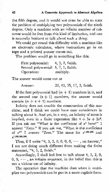
the fifth degree, and it would not even be able to state
the problem of multiplying two polynomials of the ninth
degree. Only a machine with an infinite number of col-
umns would be free from this kind of limitation, and one
is naturally hesitant to talk about such a thing.
We could get round this difficulty with a machine like
an electronic calculator, where instructions go in on
tape and a printed answer comes out.
The problem would go in something like this.
First polynomial: 4, 3, 2, finish.
Second polynomial: 5, 7, 1, finish.
Operation: multiply.
The answer would come out as
Answer: 20, 43, 35, 17, 2, finish.
If the first polynomial had (m 1 ) numbers in it, and
the second one (n -J- 1) numbers, the answer would
contain (m + n 4- 1) numbers.
Infinity does not trouble the construction of this ma-chine, and I think we could have easy consciences in
talking about it. And yet, in a way, an infinity of zeros is
implied, even in a finite expression like 4 + 3x + 2x 2.
If you ask me “What is the coefficient of x 3 here?” I
answer “Zero.” If you ask me, “What is the coefficient
of x4” I answer “Zero.” The same for x1,000 ’000 and^1,000,000,ooo^
Thus, if I write “4, 3, 2, 0, 0, 0, 0,• •
•,on forever,”
I am not doing much different from making the finite
statement, “4, 3, 2, finish.”
Accordingly, I shall feel free to talk about 4, 3, 2, 0,
0, 0,• •
•,an infinite sequence, in the belief that this is
not a vicious use of infinity.
The operation that the machine does when it multi-
plies two polynomials can be put in a more explicit form.

Arithmetics and Polynomials 43
If you look at the number ay -J- bfi + ca that occurs in
the product of
a b c
a (3 y
you may observe a pattern in it. This pattern can be felt
in the muscles, if you put a forefinger on the Latin letter
and a thumb on the Greek letter of the rows above, for
each term, as you read ay T b(3 4~ ca - Your finger will
move forward through a, i, c as your thumb moves back-
ward through a, (3, y.
A pattern of this kind appears most clearly if suffix
notation is used. The product of
pO pi p2
qo qi qi
contains the following numbers
poqo,
poqi 4- piqo,
poq2 4" piqi 4~ p2q2,
piq2 + p2qi
,
p2q2-
Question: What do you notice about the suffixes here?
If we multiply
po pi p2 * ** Pm
by
qo qi ?2* ’ * ' ’
' qnj
how can the resulting numbers be expressed most com-
pactly?
Your solution to 5 this question will, I am sure, be equiv-
alent to the following.
Let the product be ko, k\, • ••
,km+n . Then
ko = poqo,
ki = poqi + piqo,
ki — poq2 4" piqi 4“ P%qo, and so on.

44 A Concrete Approach to Abstract Algebra
In h the suffixes add up to zero, in ki they add up to 1,
in k2 to 2, and so on. In kr we expect the indices to addup to r. If p s occurs in kr ,
its partner must be qr_s . Weare thus led to write
.<? — r
kr ~ ^ ^psC/r—s-
s = 0
It is understood, of course, that for s > m, p„ = 0 andfor t > n, q t = 0. This corresponds to our remark that
in the first row pm is followed by endless zeros, and sim-
ilarly for qn in the second row.
We have now arrived at a fair specification of a poly-
nomial machine. A polynomial machine contains col-
umns into which we can enter numbers of the field F.
By “a polynomial of degree m” we understand that the
machine is set so as to show “po, pi, pi,• •
•, pm finish”
or, equivalently, “p0 , pi, pi,• •
•, pm , 0, 0, 0,
• •• ,” the
zeros continuing forever. The input to the machine con-
tains spaces for two polynomials, the first and second poly-
nomials, say (po, pi, pi,• • •) and (qQ , qh q2 ,
•)• Theoutput of the machine shows two polynomials, namelythe sum and product of the input polynomials. The sumis the polynomial (jo, ji, ji,
• •• ), where jr = pr -\- qr . The
product is the polynomial (k0 ,ki, k2 ,
• • •), where
s = r
kr = ^ ] psqr—8-
s = 0
The sum and product are defined for this new ma-chine. We cannot immediately identify sum on the newmachine with + on the old, nor product on the newwith • on the old. No doubt there is some relationship,
but until we have established what it is, we had better
use new signs for the new machine. I will use S for sum,
P for product.
The old machine is a calculating machine for the

Arithmetics and Polynomials 45
arithmetic of the field F. It adds and multiplies individ-
ual numbers.
The new machine deals with sequences such as (4, 3, 2,
0, 0, 0, • • •) and (5, 7, 1, 0, 0, 0,• • •). It gives results
such as
(4, 3, 2, 0, 0, 0,• • •) S (5, 7,1,0, 0, 0, •)
= (9, 10, 3, 0, 0, 0, ..•)
and
(4, 3, 2,0,0, 0,-)P(5, 7,1,0, 0,0, •••)
= (20, 43, 35, 17, 2, 0, 0, 0,•
We have noted above the rules by which the answers
to ( ) S ( ) and ( ) P ( ) are obtained.
It is important to note that nothing is stated about the
new machine except that it carries out these rules cor-
rectly. Nothing else whatever is assumed about the op-
erations S and P. We know that the operations S and Pcan be carried out, because they depend simply on the
operations of arithmetic in the field F. The old machine
does arithmetic; the new machine will contain one or
more replicas of the old machine, for doing the necessary
arithmetic.
The two machines, the arithmetic machine (the old
machine) and the polynomial machine (the new ma-chine), are now set up. Their nature is determined. Wecannot introduce any more assumptions. We can only
observe the machines and see what they do. We have no
more control over events. The machines must speak for
themselves.
We can however introduce certain abbreviations. It
will be convenient to have a short name for the sequence
(1, 0, 0, 0,• • •)• We shall call it 1. 1 is not the number 1.
It is not a number at all; it is a sequence. In the same
way 4 is a convenient abbreviation for the sequence
(4,0,0, 0, •••)

46 A Concrete Approach to Abstract Algebra
The sequence (0, 1, 0, 0, 0,• •
•) will also receive a
name. If you think of how we originally arrived at these
sequences, you will see what part this sequence is destined
to play. It is the sequence we should use to represent the
algebraic expression x. At last x is coming into the
picture.
We accordingly define x as standing for the sequence
(0,1,0, 0,0, •••).
In case you think anything mysterious is involved in
saying that 1 is a name for (1, 0, 0, 0,• •
•) and * is a
name for (0, 1, 0, 0, 0,• •
•)> it may help you to see howsimply these abbreviations can be embodied in the
machine. All it means is that the operator has keys on
which are written 1, 4, x, etc. If the operator presses 1,
automatically the sequence (1, 0, 0, 0,• • •) appears. If
the operator presses 4, then (4, 0, 0, 0,• • •) appears. If
the operator presses the key marked x,then (0, 1
, 0,
0, 0,• • •) will appear.
Suppose, for instance, that in setting up the first poly-
nomial the operator simply presses the key marked x,
and does the same for the second polynomial. The ma-
chine will carry out the operations S and P and we shall
see the following.
First polynomial, x, (0, 1, 0, 0, 0,• • •)
Second polynomial, x, (0, 1, 0, 0, 0,• • •)
Sum (0, 2, 0, 0, 0,• •
•
)
Product (0, 0, 1, 0, 0,• • •)
You should check for yourself that the rules, by which
the machine works, do lead to the results shown above.
Thus (0, 0, 1 , 0, 0,• •
• ) has turned up as the result of
multiplying X and x. It seems natural to provide a key
marked x 2 that will automatically set up (0, 0, 1, 0, 0,
• • •). We shall then be able to note the result, which
the machine gives us as
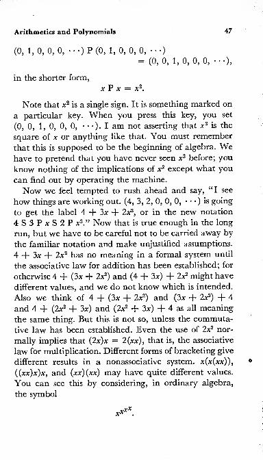
47Arithmetics and Polynomials
(0, 1,0, 0, 0, •••)P(0, 1,0, 0, 0, •••)
= (0 ,0 , 1
,0
,0 ,
0,
• • •),
in the shorter form,
X P X = X2.
Note that x 2is a single sign. It is something marked on
a particular key. When you press this key, you set
(0, 0, 1, 0, 0, 0, •••)•! am not asserting that x 2is the
square of x or anything like that. You must remember
that this is supposed to be the beginning of algebra. Wehave to pretend that you have never seen x 2 before; you
know nothing of the implications of x2 except what you
can find out by operating the machine.
Now we feel tempted to rush ahead and say, “I see
how things are working out. (4, 3, 2, 0, 0, 0,• • •) is going
to get the label 4 + 3x + 2x2,or in the new notation
4S3PxS2P a:2.” Now that is true enough in the long
run, but we have to be careful not to be carried away by
the familiar notation and make unjustified assumptions.
4 + 3x + 2x 2 has no meaning in a formal system until
the associative law for addition has been established; for
otherwise 4 + (3x + 2x2) and (4 + 3x) + 2x2 might have
different values, and we do not know which is intended.
Also we think of 4 + (3x -j- 2x2) and (3* + 2x2) + 4
and 4 + (2x2 + 3x) and (2x2 + 3x) + 4 as all meaning
the same thing. But this is not so, unless the commuta-
tive law has been established. Even the use of 2x2 nor-
mally implies that (2*)* = 2(xx), that is, the associative
law for multiplication. Different forms of bracketing give
different results in a nonassociative system, x(x(xx)),
((xx)x)x, and (xx)(xx) may have quite different values.
You can see this by considering, in ordinary algebra,
the symbol
x***.

48 A Concrete Approach to Abstract Algebra
“To the,” as used in “a to the is a nonassociative
operation. Without some convention or bracketing, xx*X
could have several meanings.
(i) We might begin at the bottom and work up. Our
calculation proceeds thus: (xx)x = x(x^), and (xx^)
X
= x(*3).
(ii) We might bracket thus (**)'*'• This equals
**(**) = *(**+ 1).
(iii) Finally we might work from the top down. This
is the meaning normally attached to xxxX
since both (i)
and (ii) lead to answers that could be written moresimply.
Working from the top down, for example, with 22^
would give 22 = 4, 2(2^) = 2^ = 16, and finally 22^
= 216.
Thus bracketing is needed to give a definite meaning to
“x to the x to the x to the x,”
and we must show good reason for it if we are going to use
“x times x times x times x”
without any brackets.
We must in fact establish the five basic laws of algebra,
which are usually written
(I) u + v = v 4" u
(II) u-v = vu(III) u 4- (v -fi w) — (u + v) + w(IV) u-(vw) = (uv)w
(V) u(v + w) = (uv
)
+ (uw).
We have to establish these laws for polynomials, (se-
quences) u, v, w. We have agreed to use and • for

Arithmetics and Polynomials 49
operations on the old calculating machine (the arith-
metic of the field F). On the new calculating machine
(for polynomials over F), we have the operations S and P,
and we must write the laws corresponding to (I) through
(V) with these symbols thus
(I') u S v = v S u
(II') u P v = v P u
(III') u S (v S w) = (u S v) S w(IV') u P (v P w) = (u P v) P w(V') u P (v S w) = (u P v) S (u P w).
At least, we must do this if we want to be consistent. But
the laws in the form first given, with -j- and •,look much
more familiar and can be read at a glance. We can be
forgiven if we sneak a look at them, to remind us of the
part that laws (I') through (V') play.
We are of course forced to use different signs for ad-
dition and multiplication on the new machine; other-
wise we should find ourselves assuming things in algebra
that in fact we had only proved for arithmetic. Later,
of course, when everything has been shown to work
properly, we shall abandon P and S and replace them
by • and -j- for future use.
Now we are not in much doubt that laws (I') through
(V') will work for polynomials, because, ifyou look back,
you will see that we defined the operations S and P so
that they gave a formal statement of what we do anyway
in school algebra.
There is, however, one point to watch. While, in illus-
trations, I have been using the numbers of ordinary
arithmetic—for example, 4, 3, 2, 0, 0,—the whole object
of our present work is to show that we can build an
algebra on any arithmetic. By an arithmetic here I mean
a field F, a set of symbols obeying axioms (7) through
(72). Now it might be that, in formulating these axioms,

50 A Concrete Approach to Abstract Algebra
we have overlooked some important property. To makesure that this is not so, we have to prove that our algebra
works properly, without appealing to anything except
axioms (7) through (72). If we can carry this proof
through, then we know that axioms (7) through (72)
not only express interesting properties of a number sys-
tem, but that they contain all the conditions an arith-
metic must satisfy if an algebra of polynomials is to be
based on it.
It is for this reason that some rather cautious formal
work is now in order. We cannot say, “It’s a waste of
time to prove such results in detail. Anyone can see that
the results are true, and only drudgery is needed to carry
the checking through.” The value of this formal work is
not that it makes us more sure of the correctness of ordi-
nary algebra but that it opens a whole new world to us.
It assures us that if we have a system of elements, an
arithmetic, we have only to verify that it satisfies the
twelve axioms of a field, and then we shall be able to
make algebraic calculations, on the basis of this arithme-
tic, without learning any new habits.
We now proceed to prove laws (I') through (V'), for
polynomials over any field F. (See the comments on
page 3 of the introduction before reading farther.)
theorem (i'). If u and v are polynomials over F, then
u S v = v S u.
Proof. Let u be the sequence (a0 ,ah a2,
• *• ) and v the
sequence (b0 ,bh b2 ,
• * •). It is understood here that is
an element of F, and that for i > m, ai = 0. In the same
way, b i is an element of F, and if i > n, b t = 0.
Let u S v be (e0 , ei, e2, • •• ) and nSwbe (<70 ,
d\, d2 ,•
•• )
.
The definition of sum was given earlier. To find u
S v, we take pr = ar, qr = bT in this definition. We find
er — ar ~f- br for all r. To find v S w, we put pr — b r>
qr = ar in this definition.
Arithmetics and Polynomials 51
We find dr = br + ar for all r. But ar and bT are ele-
ments of F. By axiom (3), a r -f- br = br + aT .
er = dr for all r.
Therefore the sequences (<?0,eh e2, • •
• ) and (d0 ,dh d2 ,
• • •) are identical, u S v = v S u. Q.E.D.Although we have not mentioned it in this proof,
axiom (7) is really involved here. Axiom (7) states that
a + b is defined for all elements a, b of F. Without this
axiom, the definition of S would be meaningless.
In the same way, the definition of the operation Puses equations such as k2 = p0q2 + Mi + Mo- This
equation has a meaning only in virtue of: axiom (2),
which allows us to speak of the products p0q2, piqi, p2qo‘,
axiom (7), which allows us to add these; and axiom (5),
which allows us to omit brackets in the addition.
theorem (n/
). If u and v are polynomials over F, then
«P V = V P u.
Proof: Let u P v be (/„, fi, f2,• • •) and v P u be
(go, gi, g2 ,•
• •)• We use the same symbols, (a0 ,ah a2 ,
• • •)
for u and (b0 ,bh b2,
• •) for v that were used in proving
the preceding theorem.
In the definition of a product, let p { = a { and q { — b {
for all i. Hence, writing the summation in full, wehave
fr — Mr + 0.\br-\ -j~ a2br—2 +•••-{- Mo-
Similarly, on putting pi = b { and q t = a {,we obtain
gr — b0ar -f- Mr-i + b2ar-2 + • •• + Mo-
By axiom (3), Mr + Mr-i = Mr-i + Mr- Using this
axiom repeatedly, we can get Mr as the last term in the
expression for gr instead of the first. We can similarly
work the termMr-i into the last place but one, by use of
the same axiom. We can continue to rearrange the terms
ofgr until the order has been completely reversed. Hence

52 A Concrete Approach to Abstract Algebra
by repeated use of axiom (3), with axiom (5) in the back-
ground to justify the omission of brackets, we find
gr = brao + b r-\d\ + • •• + b\dr—\ -j- bodr .
In each product, now use axiom (4).
gr = d0br + d\br-1 + • •* + dr—]b\ + drbo = fr .
Hence u P v = v P u. Q.E.D.
THEOREM (ill') . U S (v S w) = (u S v) S W.
Proof. Let u be («o, cl\, <22 ,
• ••), v be (bo, bi, bi, • •
•),
and w be (t0 ,c\, Ci, •••)•
u S (v S w) implies that we first combine v and w, andthe result of this is combined with u. v S w is (bo + co,
bi + ci, bi + d, • •• ) • Hence u S (v S w) is
(ao + [bo + Co], a,\ + \b\ + c{\, d2 + [bi + C2], • • •)•
We now calculate the quantity on the right-hand
side of the equation.
u S v is
(do + bo, a\ + b\, d2 + bi, •••)•
(u S v) S w is
([<zo + bo] + Co, \d\ + b\] + ci, [di + bi] + Ci,• • •).
By axiom (5), a, + (b t + c l) = (d { + b %) -f a for all i,
and hence the sequences are identical.
u S (v S w) = (u S v) S w Q.E.D.
THEOREM (iv') . U P (v P w) — (u P v) P W.
Proof. We keep the symbols for u, v, w that were used
in proving the preceding theorem.
v P w is the sequence
(boCo, boC\ -f- b\Co, boCi + b\C\ + biCo,
boCz + b\Ci + biCi + b$Co, •••)•
u P (v P w) will thus be the sequence (ho, hi, hi, hs ,
• • •),
where

Arithmetics and Polynomials 53
ho — aQ(boCo),
hi — ao(boC\ + b\Co) + a\(boCo),
h = ao(boC2 + bid + b2c0) + di(boCi + bic0)+ d2 (boCo),
and so on.
We arrive at (u P v) P w by seeing that (u P v) is
(dobo, dobi + aibo, dob2 + aib\ + d2bo,
dobz~\~ d\b 2 -f* d2bi + azbo, • * •)•
So (u P v) P w is (ko, kh k2,• •
•), where
ko — (d0bo) Co,
hi = (dobo)ci -f- (d0bi -f- dibo)co,
k2 = (dob^)c2 + (dobi + dib0)ci + (d0b 2 + dXbi + d2b0)co,
and so on.
Now, in these particular cases, it is easy to multiplyout the expressions for ho, hi, h2 ,
and ko, kx , k2 and see thatequal expressions result, ho, h, h2 can be multiplied outdirectly by appealing to axiom (7). We cannot applyaxiom (7) directly to finding kx and k2 ,
since axiom (7)deals with a(b + c). It says nothing about (b -f- c)d !
But this does not delay us for long.
For (b + c)d = a(b + c), by axiom (4)
— db + dc, by axiom (7)
— bd + cd, by axiom (4).
It is easy to deduce that
(b + c + d)d = bd + cd + dd,
since b + c + d = (b + c) + d. The result above has tobe used twice. Similarly we prove
(b + c + d + • •• + j)a = bd + cd + dd + • •
• + ja.
We can thus verify ho = ko, hi = kh h2 = k2 . Thismakes it plausible that hr = kr for all r, but of courseit does not prove that it is so. It would require an eternityto work out all the individual results. To finish our proofwe must find some way of describing hr and kr ,
from whichit will become evident that hr = kT for all r.

54 A Concrete Approach to Abstract Algebra
If you look at fa you will notice that the suffixes of a,
b, c add up to 2 in each term. In fact, fa contains all the
terms a sb tcw for which .r + t + w = 2, and each combina-
tion 5,
t, w occurs once only. The same is true of fa.
(There is nothing surprising about this result. It pro-
vides, in fact, a method of elementary algebra for mul-
tiplying polynomials.)
In general, we can show that both hr and kr are equal
to 'La sb tcw over all j', t, w for which s + t w = r.
The only difficulty in giving a proof of this result is a
difficulty very characteristic of logical analysis. There is
a stage when the facts to be proved are so evident that
you do not know just how much commentary is called
for. One faces this kind of difficulty, for instance, if
asked to prove 4 + 5 = 9. If someone questions 4 + 5
being 9, we wonder what he accepts that will serve as a
basis for the proof.
The same kind of difficulty arises here. It is pretty
evident that hr does contain all the terms a sb tcw such
that + t + w = r. The difficulty is to see just what one
must say to justify it. The simplest course is to write,
“Obviously it is so.”
I think what we have to establish is the following.
(i) If s + t + w — r, a sb tcw occurs in the expression
for hT .
(ii) It occurs once only. (Note that aibtfs is not the
same as a2b3c\. Both of these will occur in fa.)
(iii) No term occurs in hr other than the type men-
tioned in (i) above.
The same of course must be proved for kr .
Conditions (i), (ii), and (iii) are easily verified. Let
DPwbe (jo, ji, ;2,
• • •)• Then, by the definition of P,
ji = boCi + biCi-i + b2Ci-2 + • •• + biCQ.
Since u P (v P w) is (fa, fa, fa, •• •), we have

Arithmetics and Polynomials 55
hr = a0jr + ai/r-1 + jr—2 + * ** + Orjo-
We want to prove, for (i), that if .$• + f + a; = r, then
a sb tcw occurs in hr .
Now hr contains a sjr-s • As r — s = t + w, a sjr-s =cisjt+w jt+w contains b tcw . Hence the term a sb tcw does
appear in hr . (It cannot cancel, since no negative terms
are involved.)
Next, for (ii), we must show that a sb tcw occurs once
only. In hr ,a s occurs only in a sjT-s
* And jr-s,that is,
jt+w, contains only one term involving b t,namely b tcw .
Thus a sb tcw cannot occur more than once.
Finally, we prove (iii). hr is the sum of expressions
a sjr- s ,and jr- s is the sum of terms b tcr-s-t Hence every
term appearing in hT is of the form a sb tcr-s-t
,
that is to
say, of the form a sb tcw where r — s + t + w.
We have now completed the proof that hr is as stated.
A similar argument can be carried through for kr . Hence
hr — kr for all r, and Theorem (IV') is proved. Q.E.D.
THEOREM (v') . U P (v S w) = (u P v) S (u P w)
.
Fortunately the proof of this theorem is much shorter.
It consists simply of a direct verification.
v S w is the sequence (b0 + c0 ,bi + c\, 62 + ^2,
’ ’ ’)•
u P {v S w) is then (y0 , yi, yz,’ • •), where
Jr = Go{b r + Cr) + a\(b r-l + Cr-1) + - * - + Gr(^o + A))-
On the right-hand side, u P v is (/o, fi, f2,• •
•)> where
fr = aob r + a\br-\ -(-•••+ a rbo.
«Pa)is (zoj z\, Z2, •• •), where
Zr — GoCr “t“ CL\Cr—\ OrCt).
* The trouble with this kind of analysis is that you start asking
yourself, “How do I know that as only occurs once? Ought I to
prove that it does?” Every analysis must stop somewhere. Wemay as well be firm. We have no doubt that the statement just
made is true. We stop here. Future generations can get their
Ph.D.’s in mathematical philosophy by analyzing this statement
if they want to.

56 A Concrete Approach to Abstract Algebra
The theorem requires us to show that yr = fr + zT for
all r. But
fr + zr = (aobr + af)r-\ + • •• + arbo)
+ (floCr + d\Cr—\ + * ** + drcf)
— (dobr + aoCr) + (d\br-\ + fliCr-l) + • • *
+ (arbo + a rco) by repeated use of axioms
(3) and (5),
— do(br + Cr) + d\(br-\ + Cr-1) + * * *
+ ar(b0 + co) on applying axiom (7) to each
bracket,
= yr-
Hence the theorem is proved. Q.E.D.
In these proofs it will have become apparent that
many of the steps we take in algebraic calculations can
be justified by appeal to the commutative, associative,
and distributive laws. We began by assuming these for
the arithmetic of the field F;we have now shown, by
establishing (I') to (V'), that these same principles also
hold for polynomials over F. This allows us to relax our
vigilance somewhat. We now know that it is quite justi-
fied to assume for polynomials u, v, w that uv may be
replaced by vu,that u(v + w) may be multiplied out as
uv + uw}that uvw has a meaning without any need for
brackets.
We next proceed to put the theory into a more famil-
iar form. We have already introduced the abbreviations,
1 for the sequence (1, 0, 0, 0,• •
•),
and x for (0, 1, 0, 0, • • •),
and x 2 for (0, 0, 1,0, • • •).
definition. xn stands for the sequence with pn — 1, all
other pi zero.
Note here that pr = 1 refers to the element 1 of the
field F. The n that occurs in pn and x", however, is an
ordinary counting number of our everyday arithmetic.

Arithmetics and Polynomials 57
For instance, in the arithmetic modulo 5 with the ele-
ments O, I, II, III, IV, we still consider sequences such
as (II, I, III, O, IV, II, I, O, O, • • •) with p0 = II,
pi = I, p2 = HI, p% = 0,pk = IV, p5 = II, p 6 = I, and
we can consider II - II - II * II * II * II * II = II 7. Thus, even
though the arithmetic modulo 5 only contains the five
distinct elements O, I, II, III, IV, yet the ordinary
numbers, including the numbers 5, 6, 7,• •
•,cannot be
kept entirely out of it. This might cause complications
in the Pacific Island experiment (p. 18).
THEOREM. Xm P Xn — Xm+n .
Proof. Let xm be (p0 , pi, p2,• • •) where pm = 1, all
other elements being zero.
Let xn be (q0 , qi, q2 ,• • •) where qn = 1, all other ele-
ments being zero.
If xm P xn is (£o, k\, k%,
• ••), then
r
kr = ^ ] p&qr—fs = 0
The term p sqr-s will be zero if either ps or qr-s is zero.
p s is non-zero only for s — m, and qr- s is non-zero only
if r — s = n. Hence a non-zero term occurs on the right-
hand side only if s = m and r — s = n; that is, only if
r = m + n. Hence kr is zero except for r = m + n, and
km+n = 1 •
But km+n =1, all other kr zero is the sequence for
Xm+n
xm P xn = xm+n . Q.E.D.
Theorem. If a is any element of F, and a denotes the se-
quence (a, 0, 0, 0,• • •) then aP / is the sequence (0, 0,
• ••
,
0, a, 0, 0,• •
• ) ;that is, axn is the sequence defined by pn = a,
all other pi = 0.
Proof. Calculate a P xn . Verification is immediate.
theorem. Every polynomial can be written in the form
p0 S (pi P x) S (p2 P x2) S • • • S (pn P x").

58 A Concrete Approach to Abstract Algebra
The meaning of this theorem can be appreciated most
easily if, for a moment, we replace S, the sum sign, by
the usual +, and P, the product sign, by • . The expres-
sion above then becomes
pO + pi'* + P2-*2 + * •
• + P»-*"-
Proof. Since pa is (po, 0, 0, 0, 0,• •
•), while by the pre-
vious theorem
px P * is (0, pi, 0, 0, 0,• • •),
p2 P *2is (0, 0, p2, 0,0, • • •),
and so on, it is evident that (po, pi, pi, po, • ••
, pn , 0, 0, 0,
• •• ) can be obtained by summing the terms above.
Q.E.D.
Thus, apart from the fact that the unfamiliar S and
P are playing the parts of+ and •,we have now reached
a stage where polynomials can be written down in the
ordinary way, and added and multiplied; we know that
the commutative, associative, and distributive laws, (I')
through (V'), hold—that is to say, that the processes
behave as in ordinary algebra.
There is, however, one remaining point. We seem nowto have two distinct subjects. In terms of our machinery,
we have one machine for adding and multiplying the
elements of F—the numbers of the arithmetic. This is
the old machine. The new machine deals only with se-
quences, with polynomials. The two machines seem quite
distinct; no cables pass from one to the other. This seems
a little peculiar, for surely an arithmetic and its algebra
should be connected?
In our ordinary algebra we speak of a quadratic poly-
nomial such as 4 + 3* -f- 2x2, a linear polynomial such
as 4 + 3x, and a constant polynomial such as 4. Thus, one
and the same sign, 4, is used for the number 4 and the
constant polynomial 4. Nor does this cause any trouble.
Arithmetics and Polynomials 59
Most people in fact are hardly aware that any such dis-
tinction can be made. Probably this distinction is in-
volved in the trouble that some students find in drawing
the graph of y = 4. They seem to be helped by the sug-
gestion that they should draw the graph ofy = 4 + 0 • x,
which brings out the kinship of y = 4 to the family of
linesy — mx -f- c, or reminds the student of the procedure
for tabulating values and drawing the graph. The psy-
chological effect of writing y = 4 as y = 4 —f- 0 • at seems
to lie in emphasizing that 4 can be regarded as a par-
ticular case of a polynomial.
How does this overlapping of number behavior and
polynomial behavior appear on our machines? Let a and
b be any elements of F. On the arithmetic machine, wecan find a + b and a-b. What will happen if, on the
polynomial machine, we find a S b and a P b?
a is {a, 0, 0, 0,• • •)•
b is (b , 0, 0, 0,* * •)
The rules for S and P give
a S b is {a -j- b, 0, 0, 0,• • •).
a P b is (ab, 0, 0, 0,
• • •)•
Thus
a S b = (a + b),
a P b = (ab).
For example,
2 S 3 = 5,
2 P 3 = 6.
This means to say, we can do our arithmetic on the
algebra machine.
2 S 3 = 5 means that the polynomial 2 added to the
polynomial 3 gives the polynomial 5; this runs exactly
parallel to the relation between numbers, 2 + 3 = 5.
This parallelism is an example of isomorphism. The struc-
€0 A Concrete Approach to Abstract Algebra
ture, the pattern, of numbers is exactly the same as the
structure, the pattern, of constant polynomials.
Accordingly, it becomes something of a luxury to ownboth a polynomial machine and an arithmetic machine.
Since we can do all our calculations on the polynomial
machine, we can trade our arithmetic machine in. When-ever we want to do an arithmetical calculation aboutnumbers a, b, c, we can set up the polynomials (a, 0, 0,•
'
(b , 0, 0,• *
•), (c , 0, 0,• • •) and infer the arithmet-
ical result from operations on the polynomial machine.
Getting rid of the arithmetic machine is welcome. Wehave so far had to use S, P, and +, • to avoid confusion
between operations on polynomials (sequences) and op-
erations on numbers. But now that the arithmetic ma-chine has gone, there is no longer a need for this distinc-
tion. We can write the familiar + where S stood on the
machine, and • for P. We can also drop the distinction
between the number a and the constant polynomial a.
In effect, the sequences (p0 , ph p2 ,• •
•) and the opera-
tions S and P are now relegated to the interior of the
machine. On the outside of the machine we see (if ordi-
nary numbers compose the field F) 0, 1, 2, 3, and so on;
+ and •; *, x2
,x 3
,and so on.
If we press 4 -f- 3-x + 2-x 2,then, in some space inside
the machine, the sequence (4, 3, 2, 0, 0, 0,• • •) will ap-
pear. If we simply press 4, the sequence will be (4, 0, 0,
0, • • •)• When the operation + is required, the machinecarries out S in its interior; when • is required, the ma-chine carries out P.
Note that * has not changed its meaning at all. Whenwe press x, the machine sets up (0, 1, 0, 0, 0,
• • •) in its
interior. That is all we know about x. There is no re-
quirement that * be an element of F, a number, or any-
thing of that sort.

Arithmetics and Polynomials
Substituting a Value for x
61
Have we perhaps gone too far? After all, we still wantto say that x 2 — 3x + 2 = 0 if * = 1 or x — 2. What are
we to do when we want to substitute x — 2 or x = k in
a polynomial po + p\x + — + pnxn?
xm has been defined by the sequence (0, 0, 0,• •
• ,0,
1 , 0, 0, 0,• •
• ) that it produces in the machine. However,
the theorem we had earlier, which we now write xm -xn
— xm+n gives us another way of regarding xm .
We have seen earlier that x2 — x-x. Hence
x3 = x1+2 = x-x2 = x-x-x,
x4 = x1+3 = x-x3 = x-x- x-x,
and so on. The cubic polynomial
a -f- b-x + c-x2 + d-x3
could thus be written
a -f- b-x + c-x-x + d-x-x-x.
In what relation does this stand to the expression
a + b-k + c-k-k + d-k-k-k,
where k is an element of F?
Let us think what happens in the interior of the ma-chine when these two things are calculated:
a produces (a, 0, 0, 0, 0, 0, 0, • • •),
b-x produces (0 ,b, 0, 0, 0, 0, 0, • • •),
c-x-x produces (0, 0, c, 0, 0, 0, 0, — ),
d-x-x-x produces (0, 0, 0, d, 0, 0, 0, • • •).
Summing a + b-x + c-x-x + d-x-x-x produces (a, b, c,
d, 0, 0, 0, • •• ) as, of course, we could have foreseen. On
the other hand,

62 A Concrete Approach to Abstract Algebra
a produces {a, 0, 0, 0, 0, 0, 0, • • •)>
b-k produces {bk, 0, 0, 0, 0, 0, 0, • •)>
c-k-k produces (ck2
, 0, 0, 0, 0, 0, 0,• • •)>
d-k-k-k produces (dk3, 0, 0, 0, 0, 0, 0,
• • •).
Summing a + b-k + c-k-k + d-k-k-k produces
(a + bk + ck2 + dk\ 0, 0, 0, 0, 0, 0,• • •)•
It will be convenient to use the abbreviation /(x) for
a + b -x + c-x-x + d-x-x-x, and f{k) for a + b-k +c-k-k + d-k-k-k.
These look very much alike, but they appear very
differently on the machine. /(x) appears as (a ,b, c
,d,
0, 0, 0,• •
•), a polynomial of degree three, specified by
the four elements a, b, c, d of F. f(k) appears as (e , 0, 0,
0, 0, 0,- - •), where e — a + b-k + c-k-k + d-k-k-k is
a single element of F. We can regard f(k) as a constant
polynomial or, if we like, we can identify it with the ele-
ment e of F; we agreed earlier to neglect the distinction
between e, the constant polynomial (e , 0, 0, 0,• •
•) and
the element e of F.
In ordinary high school algebra we meet the idea of
“substituting k for x.” On our calculating machine we
accordingly must introduce a key marked, “substitute
k for x.”
If the calculating machine is carrying the sequence
(a, b, c, d, 0,0,0, - -- ) which represents /(x), and we press
the “substitute k for x” key, the machine will compute
e = a + bk + ck 2-f dkz—this is a single number, an
element of F—and will set up the sequence (e
,
0, 0, 0,
0,0
,•••).
This explains and defines what we mean by “substi-
tute k for x.” If on a machine you see a knob marked
with an unfamiliar word, and you want to understand
the meaning of this word, all you need do is turn the
knob and observe what happens in the machine. When

Arithmetics and Polynomials 63
you are completely familiar with, what this knob dogs,
then you understand the word written on it. There is
nothing more to understand.
I emphasize this because there is much discussion at
present of the correct use of words. People are worried
about whether they really understand what a word
means. Some philosophers hold that successful thinking
is only possible after all words have been defined exactly.
It may be that some people actually do think by means
of words. If so, they are a minority. Most people think
by imagining, by picturing actual objects, actual proc-
esses, actual happenings. We speak to each other in order
to make sure that we are thinking of the same thing and
picturing it in the same way. We clear up confusion in
our own minds by thinking about something until we
have a clear picture of it.
The idea that a word or a symbol has one fixed, exact
meaning is dangerous even in mathematics. Poincare,
one of the greatest modern mathematicians, declared
“Mathematics is the art of calling different things by
the same name.” We have had an example of this
already. We used + originally in arithmetic with
3 -}- 4 = 7 . When we got to dealing with the arith-
metic modulo 5,we could have brought in a new sign
of combination and written, perhaps, III © IV = II.
But we found it more convenient to write 3 + 4 = 2.
2,3
,4
,and + all have new meanings here, but we find
it convenient to use the same signs. When we were
dealing with sequences, we used a new sign S for sum,
3 for (3, 0, 0, 0,• * ), and 4 for (4, 0, 0, 0, 0,
• • •)• Wewere glad, though, when we stopped writing 3 S 4 = 7
and went back to 3 + 4 = 7 for constant polynomials.
So we have already used + in three different senses.
When we use a sign, then, it does not imply that all its
meanings are exactly the same, but that there is enough

€4 A Concrete Approach to Abstract Algebra
in common to make the family resemblance worth
emphasizing.
I should certainly not advise anyone teaching
ninth-grade algebra to say that x is the sequence
(0 ,1
,0
,0
,0
,
Earlier we discussed the question of the polynomial
x 2 + x over F, the field consisting of 0, 1 modulo 2. Wasthis polynomial equal to zero or not? We have two sets
of facts:
(i) The polynomial x 2 + x is the sequence (0, 1, 1, 0,
0, 0,• • •). The constant polynomial 0 is the sequence
(0, 0, 0, 0, 0, 0,• •
• ) • These two sequences are distinct.
In this sense, x2 + x 5^ 0.
(ii) If in x2 + x we substitute 0 for x, we get 0 2 + 0,
that is, 0. If we substitute 1 for x we get l2 + 1, which
is also 0. 0 and 1 are the only elements of F. Hence for
every k of F, k 2 + k = 0.
It is desirable that we should have some way of indi-
cating whether we are posing questions, or making
statements, in the sense of (i) or (ii). We might makesome sort of convention about the use of letters; wemight always use x for sense (i), and k for sense (ii).
This might be inconvenient at times; it is surprising howsoon the letters of the alphabet get used up in a mathe-
matical discussion.
It is better to have some terminology to indicate howa symbol is being used. When we write k 2 + k = 0 to
mean that if any element of F is added to its square, the
result is zero, we say that A: is <2 variable. When we write
x 2 + x without caring what x may mean or whether it
means anything at all, simply as a symbol obeying cer-
tain formal rules, we say that x is an indeterminate.
A professor of mathematics once made the following
criticism of the remainder theorem. He said, “The re-

Arithmetics and Polynomials 65
mainder theorem states that when f(x) is divided byx — a, the remainder is f{a). But when x = a, x — a is
zero. You cannot divide by zero. That means we cannot
consider x being a when we are dividing by x — a. Theproofs of the remainder theorem that depend on a being
substituted for x are therefore false.”
This criticism is entirely incorrect. The critic is clearly
thinking of x as a variable,so that x is a number and
x — a is also a number. Let us take an example of divi-
sion and see how well or badly it works to regard x as
a variable.
Example. “When x 2is divided by x — 3, the quotient
is x + 3 and the remainder 9.” I am sure you will agree
that this is a correct statement. Let us see how it looks
when we take particular numbers for x.
x = 5. “When 25 is divided by 2, the quotient is 8
and the remainder 9.”
x = 6. “When 36 is divided by 3, the quotient is 9
and the remainder 9.”
x = 7. “When 49 is divided by 4, the quotient is 10and the remainder 9.”
There is a sense in which all of these are true. Forinstance, 25 = 2X8 + 9. Yet they represent very
strange arithmetic.
If, purely as a matter of arithmetic, we had been asked
to divide 25 by 2, 36 by 3, and 49 by 4, we would havegiven the remainders as 1, 0, 1, respectively. We could
never have arrived at the conclusion “The remainder is
always 9” by arithmetical experiments.
In fact, the sentence “When x2is divided by x — 3,
the remainder is 9” is a statement of algebra that is not
a generalization about arithmetic. The division in ques-
tion is not arithmetical division: it is division according
to the rules we learn for dealing with polynomials.

66 A Concrete Approach to Abstract Algebra
“Divide x2 by x — 3” means exactly the same as
“divide (0, 0, 1, 0, 0, 0,• • •) by (-3, 1, 0, 0, 0,
• • •)”
It does not make sense in any other interpretation.
The thing we are dividing by here is (— 3, 1, 0, 0,
0, • •
•), and this is not zero. Zero is (0, 0, 0, 0, • • •).
There is no need to take precautions to ensure that the
divisor does not become zero. (— 3, 1, 0, 0, 0, • •
•) just is
not (0, 0, 0, 0, 0,• •
•), and there are no circumstances in
which it could become (0, 0, 0, •••). A polynomial can
always be divided by x — 3 in the sense in which long
division is done in algebra.
The distinction between x regarded as a variable and
x regarded as an indeterminate is therefore not an empty
one.
We do have to distinguish between the two statements
below.
Statement I. For the indeterminate x,the polynomial
/(x) = 0. This means that /(x) is (0, 0, 0,• • *)• This
statement is true, for instance, if /(x) = — x2 + 1 +(x — l)(x + 1). When this /(x) is simplified by the rules
of algebra, the result is zero. We could express it as
(1, 0, -1, 0, 0, 0,• • •) S (-1, 1, 0, 0,
• • •) P (1, 1, 0, 0,
0, •••) = (0,0, 0,0, •••).
Statement II. For all values of the variable x, the
polynomial /(x) = 0. This means that, for every element
k of the field F, we have f(k) = 0.
What is the relationship between statement I and
statement II? We have seen that statement II is true,
with F the arithmetic modulo 2, for x2 + x. But state-
ment I is not true for x2 + x, since x2 + x is (0, 1, 1,
0, 0,• •
• ) and not (0, 0, 0, 0, 0,• •
• ) . So statement I does
not follow from statement II, at least not for every field
F. (It does follow in elementary algebra, as we noted
earlier.)
Does statement II follow from statement I? If state-

Arithmetics and Polynomials 67
ment I is true, f(x) is (0, 0, 0, 0, 0, 0,• • •)• Now (0, 0, 0,
0, 0, 0,• • •) is a particular case of (
a
,b, c, d, 0, 0, • • •)
with a = 0, b = 0, c = 0, d = 0. I have quite arbitrar-
ily chosen to regard (0, 0, 0, 0, 0,• •
• ) as a cubic, in order
to make clear that we are not involved in a discussion of
the infinite series 0 + 0k + Ok2 + 0£3 + 0£4 + • • • . Apolynomial is essentially a finite sequence. In the lan-
guage of page 42, it may be “4, 3, 2, finish.” “Finish”
means that we have reached the stage where we have
zeros only. (0, 0, 0, 0, 0,• • •) could be written “finish”;
with it we finish before we start! This makes the inter-
pretation of the procedure for substituting k slightly
obscure. If, however, we regard (0, 0, 0, 0, 0,• •
•) as
“0, 0, 0, 0, finish,” which we are entitled to do, we can
apply the rule without any difficulties of interpretation.
The explanation of “Substitute k for x” given on page 61
leads to the value e = a + bk + ck 2 + dk3 = 0 + 0&
+ 0k 2 + Ok3 = 0, whatever element of F the quantity
k may be. Hence, statement II follows from statement I.
There is an important point to notice. The explanation
of “substitute k for x” assumed that f(x) had been
obtained in the standard form, po + pix + p2x2 + • • •
+ pnxn . Substituting k for x gave po + p\k + p2k2 + • • •
+ pnkn .
If we were given /(x), say in the form
f(x) = (ao + a\x + a2x2)(bo + b\x + b2x
2),
the definition instructs us to multiply out /(x) as
^ij ^2 ,dj fij
'' P (b0 ,
b\, b2 , 0, 0, 0, ’) — (aobo,
Qob\ H- a.\bo, CLobi -f- a\b\ + a^bo, a\b2 H- Qibi, a 2b 2, 0, 0, 0,
•••),
and then to press the key “Substitute k for x,” giving
f(k) = aobo -t~ (aobi -j- a^bo) k + (aob2 + a\b\ + a^bo) k 2 +(a\b2 -f- a2bi) k3
-f- a2p2)&.
But you naturally ask, “Gould we not use the simpler
form (a0 + a\k + a 2k2)(b0 + b\k + b2k
2)?” The sugges-

68 A Concrete Approach to Abstract Algebra
tion is that multiplying out and then substituting could
be replaced by substituting and then multiplying out.
For instance, the two procedures for substituting 3 for x
in (* — 1)(* + 1) would be
(i) (x — l)(x + 1) = x 2 — 1.
Substituting 3 for x gives 3 2 — 1 = 8.
(ii) Substituting 3 for x in (x — 1) gives 2.
Substituting 3 for x in (x + 1) gives 4. 2*4 = 8.
Procedure (i) we know to be correct, for it merely carries
out the instructions of the definition. Procedure (ii) weobserve, in this example, gives the same answer as pro-
cedure (i).
Now, of course, it is not surprising that this should be
so. If you will look back to page 34, you will see that weobtained our rules for constructing the polynomial ma-
chine by considering what happens when we add and
multiply in elementary algebra. The process of our
thought has been something like this.
(I) We learn arithmetic.
(II) We notice in arithmetic various facts, such as
3 X 4 = 4 X 3 and 3 + 4 = 4 + 3. We satisfy our-
selves that these facts are particular examples of general
properties of numbers, expressed by axioms (7) through
(72). The numbers of arithmetic form a field.
(III) The processes of elementary algebra can be
justified by the field axioms. For instance, if a, b, c, d are
elements of a field F, we can show that
(a + bk) -f- (c + dk) = (a + c) + (b + d)k
and(a + bk) (c + dk) = ac + (ad + bc)k + bdk2
for any element k of the field F.
(IV) We extract from (III) the abstract pattern
(a, b, 0,0, • • •) S (c, d, 0, 0,• • •)
= (<s + c, b + d, 0, 0,• • •),

69Arithmetics and Polynomials
{a, b, 0,0, •••) P (c, d, 0, 0,
• • •)
= (ac,ad + bd
, 0, 0,• • •),
and specify, quite abstractly, our polynomial machine
for combining sequences by the operations S and P.
(V) By introducing the sign * for the sequence
(0, 1, 0, 0,• • •)> and slipping back into writing + for S
and • for P, we are able to write the equations of (IV)
in the form
(a + bx) + (c + dx) = (a + c) + (b + d)x,
(ia + bx)(c + dx) = ac + (be + ad)x + bdx2,
which look very much like the equations of (III). Whatwe have gained is that x is no longer restricted to being
a number, an element of the field F.
(VI) We verify that the sequences of (IV), and con-
sequently their expressions in the symbolism of (V), obey
the commutative, associative, and distributive laws, and
hence can be worked with in exactly the same way as
the expressions of elementary algebra.
(VII) The operations of (IV) and (V) have been
based on the patterns of (III). This means that, although
the symbol x does not have to be interpreted as an element
of the field F, yet it can be so interpreted. If, in any true
statement of (V), * is everywhere replaced by k, an ele-
ment of the field F', we obtain a true statement in the
language of (III).
The assertion (VII) may be illustrated by the follow-
ing two theorems.
theorem. If p(x), q(x), f(x) are polynomials in the inde-
terminate x over a field F, and p(x) + q(x) = f(x), then for
any element k of F, p(k) + q(k) = f(k).
theorem. If p(x), q(x), g(x) are polynomials in the inde-
terminate x over a field F, and p(x) • q(x) = f(x), then for any
element k of F, p(k) • q(k) = f(k).
By combining these theorems, we can obtain results

70 A Concrete Approach to Abstract Algebra
such as this: if
/(*) = P(x) q(x) + r(x)
for an indeterminate x, then
f{k) = p(k) q(k) + r(k)
for any element k of F.
EXERCISES
1 . Write out the proof of the remainder theorem. When anyequation is written, make it plain whether the symbols are
indeterminates, variables, or fixed elements of a field F. State
explicitly any theorems used in the course of the proof.
2. ax2 + bx + c is a quadratic over a field F in an indeter-
minate x. Explain what is meant by saying that the quadratic
has at most two roots. Prove that this statement is correct
whatever the field F.

Chapter 3
Finite Arithmetics
Earlier we considered the arithmetic of Even and
Odd. This was a particular example of an arithmetic
modulo n, namely the arithmetic modulo 2. When wewere discussing Even and Odd, we accepted many state-
ments such as “Even plus Odd equals Odd” as agreeing
with our experience of arithmetic. We did not analyze
or prove these results. To prove them is, of course, simply
a matter of elementary algebra. We now look at these
proofs as a first step toward proving the properties of the
arithmetic modulo n.
“Even plus Odd equals Odd” is a short way of saying,
“When any even number is added to any odd number,
the result is an odd number.” To prove the truth of this
statement we must translate into algebraic symbolism
the expressions “even number” and “odd number.”
If our symbols a, b,c, • ••
,x,y, z stand for integers,
the numbers 2a, 2b, 2c, •••,are even; the numbers 2a + 1,
2b + 1 ,2c + 1 ,
• ••
,are odd. Any even number can be
expressed as 2a. Any odd number can be expressed as
26 + 1. When these are added, we get 2a + 2b + 1 =2 (a + b) + 1, hence an odd number; and we have
proved the statement.
There is no difficulty in justifying the other results of
the addition table modulo 2.

72 A Concrete Approach to Abstract Algebra
The multiplication table is justified by the following
four results:
(2a)
•
(2b) = 2(2ab),
(2a) ‘(2b + 1) = 2-a(2b + 1),
(2a + l)-2b = 2-b(2a + 1),
(2a + 1) • (2b + 1) = 2(2ab + a + b) + 1.
Apart from the particular results obtained, such as
“Odd times Odd equals Odd,” this procedure shows that
the question “When an odd number is multiplied by an
odd number, is the result Odd or Even?” has a definite
answer. We do not need to ask, “Which odd numbers
are you thinking of?”
Compare the situation if we divide numbers up into
perfect squares and other numbers. One cannot answer
“yes” or “no” to the question, “When a square number
is added to a square number, is the result square?” 0 + 1
,
9 + 16, 25 + 144 are examples of results that are
squares; 1+4, 1 + 9,t4 + 9 are examples of results
that are not.
Our procedure then, in forming the arithmetic modulo
2 (and the other modular arithmetics), has been to divide
the integers up into classes in such a way that, if we knowto which classes x and y belong, we know to which classes
x + y and xy belong.
The arithmetic modulo 2 is easy to talk about because
we have two generally accepted words, Even and Odd,
to describe the classes. The language does not contain
words to express that a number is divisible by 3, or leaves
remainder 1 or remainder 2 on division by 3. We accord-
ingly have to invent symbols such as
O to label any number of the form 3a,
I to label any number of the form 3a + 1,
II to label any number of the form 3a + 2.

Finite Arithmetics 73
Similarly, we used the symbols O, I, II, III, IV for the
arithmetic modulo 5.
For example, to prove that III -IV = II modulo 5,
means to prove that (5a + 3) (5b + 4) is of the form
5c + 2, which is very easy to do. We thus show (i) that
when a number x from class III is multiplied by a num-ber y from class IV the product xy lies in a definite class,
independent of the particular numbers x and y chosen;
(ii) that the class is in fact the class II.
Of these results, (ii) is, so to speak, arithmetical. It
holds for arithmetic modulo 5, but not necessarily for
other arithmetics; for instance, in modulo 7 arithmetic,
III IV = V.
Result (i), however, has no reference to particular
numbers, and generalizes immediately to give theorem 1 .
theorem 1. If, for any whole number n, the integers are
divided into classes, so that class P contains all numbers of the
form na + p, class Q contains all numbers of the form na -f- q,
and so on; then, given only that the numbers x andy belong to the
classes X and Y, the classes to which x + y and xy belong are
determined.
We can restate this result as follows: if x\ and x2 are in
the same class, and y\ and y2 are in the same class, then
xi + y\ and x2 + y2 are in the same class, and xiyi and
x2y2 are in the same class.
Saying that xi and x2 are in the same class is equivalent
to saying that x\ — x2 is a multiple of n.
Thus we are given = nc + x2 , yi = nd + yz-
Hence *i + yi = n(c + d) + x2 + y2 and (x\ + yi)—
(x2 + yf) is a multiple of n.
Also xiyi = n 2cd + ncy2 + ndx2 + x2y2 so xiyi — x2y2 is
a multiple of n.
The theorem is proved. Q.E.D.
We have now shown that axioms (7) and (2) hold for
arithmetic modulo n. We have defined X + Y and X-Y;

74 A Concrete Approach to Abstract Algebra
namely, if x is any number of the class X, and y any
number of the class Y, then X + Y means the class to
which x y belongs, and X - Y the class to which xy
belongs. Theorem 1 assures us that this definition is
consistent.
Axioms (3), (4), (5), (6), (7) are now almost self-
evident.
Axiom (3) requires X + Y = Y X. Now T + ^ is
the class containing y + x, while X + Y is the class con-
taining x + y- But we know, for any numbers x, y, that
y + x = x + y. Call this number k. Then X -f- Y is the
class containing k, and Y + X is the class containing k.
Hence X + Y and Y + X are the same class. Q.E.D.
Axioms (4), (5), (6), (7) follow in the same way. If Zis the class containing z, axiom (7), for instance, re-
quires X-(Y + Z) = (X-Y) + (X-Z). We show that
X-(Y + Z) is the class containing x(y + z), and (X-Y)
+ (X-Z) is the class containing xy + xz. As the numbersare the same, the classes are the same.
Axiom (8), on subtraction, asserts that, for given
classes P, Q (containing the numbers p , q) the equation
P + X= Q
has one and only one solution. It evidently has a solution.
For let .S' be the class containing the number (q — p).
Then P + S is the class containing/) +(<?—/>), that is,
P + S contains q. .*. P + S = Q. S is a solution.
Suppose the class T, containing the number t, is also
a solution. P + T is the class containing p + t. If
P + T — Q, this means that/) -f- t belongs to Q. .'./) + t
= q + na for some whole number a. t = (q — p) + na.
Hence t belongs to the class S. .\ The class to which t
belongs is S. That is, T is S.
Axiom (8) is thus proved to hold.
Axiom (9) asserts that there is a class playing the role

Finite Arithmetics 75
of zero. Let O be the class containing the number 0.
P + O is the class containing the number p + 0. As
p 0 = p, P + O = P. Hence O plays the role of zero.
By axiom (8), there can only be one such class. Other-
wise the subtraction P — P would have more than one
answer.
We may as well deal with axiom (77) now. It should
be evident that the class I, containing the number 1,
plays the role of unity.
Axioms (77) and (72) do not hold for all modular
arithmetics. For instance, in arithmetic modulo 6, the
equation 11 -X — III has no solution, so division is not
possible. Also II -III = O; axiom (72) does not hold in
this arithmetic.
The class O contains all numbers of the form na + 0,
that is, all numbers na,all multiples of n. Thus “XY = O
only if X — O or Y — O” is the same requirement as
“ry is a multiple of n only if x is a multiple of n or y is a
multiple of n This property is characteristic of prime n.
Hence axiom (72) holds if and only if n is prime.
Does axiom (10) hold when n is prime? That is to say,
given classes P, Q, where P is not O, can we find a class
X such that P-X = Q?How do we go about finding such an X in practice?
For example, in the arithmetic modulo 5, how should wesolve II -X = III? We should have to look through the
II times table until we found the answer III. Here is the
two times table.
no = oIII = II
II -II = IVII -III = I
II -IV = III
If you look at the right-hand side, you will see that all
the classes O, I, II, III, IV occur there. That is to say,

76 A Concrete Approach to Abstract Algebra
we may make II -X equal to any class we like, by choos-
ing X suitably. In arithmetic modulo 5 then, division by
II is always possible.
This suggests a way of studying the arithmetic modulo
n. This contains n classes, corresponding to the numbers
0, 1, 2,• •
•,(n — 1). We take some class P, and let X
run through the n classes. If the resulting PX are all dif-
ferent, they must form a complete set of classes. By choos-
ing X suitably, we can make PX — Q for any assigned
Q. Division by P is then possible.
Can we show then that, when P is not O, all the P
X
are different? We suppose, of course, that n is prime; it
is easily seen that for n composite the result is not true.
The proof is extremely simple. It almost leaps to the
eye as soon as we state the question in algebraic symbols.
Suppose the PX are not all distinct. Then X = Uand X = V give the same result; that is PU = PV. But
(in view of the axioms already proved) this means
P{U — V) = O. But P is not O, by our assumptions.
U — Vis, not O, since U and V are not equal. Axiom (72)
has already been established. Hence P(U — V) is not O,
since neither factor is O. We thus arrive at a contradic-
tion if we assume the PX not distinct. Hence the PX are
distinct.
Accordingly, when n is prime, division is possible, for
divisors other than O. We have thus theorem 2.
theorem 2. The arithmetic modulo n, where n is prime, is
,a field.
For this arithmetic satisfies axioms (7)-(72).
You may have noticed that we proved axiom (70)
from axiom (72) and the remaining axioms. It is evident
that there is a close connection between axioms (70) and
(72). Since we proved axiom (70) from axiom (72), have
we perhaps not been extravagant in including axiom (70)
at all? Could we not simply assume (72) and deduce (70)?

Finite Arithmetics 77
For a finite field—that is, a field with a finite numberof elements—we could do so. But consider a very familiar
structure, the integers. For the integers, axioms (7)
through (9), (77), (72) hold. All the answers in the twotimes table are distinct:
-6, -4, -2, 0, 2, 4, 6, •••.
But this does not prove that every number occurs as ananswer in the two times table. In fact, 2x = 3 has nosolution in integers.
Thus for the integers, axiom (72) holds, but (70) is
false. It is thus impossible to deduce axiom (10) from (72),
the other axioms being given, without the additional
information that the structure contains only a finite
number of elements. And most of our algebra, of course,
deals with structures having an infinity of elements. Forsuch a structure, axiom (70) is a stronger assumption
than (72).
Question: If axioms (7) through (77) are given, does
Axiom (72) follow?
An Alternative Approach to Division
Our proof of axiom (10) has two limitations. First of
all, a proof has two functions. One is to establish the
particular result. This, of course, our proof does. Theother function is to throw light on similar problems, to-
suggest analogies. Our proof holds only for finite struc-
tures. For infinite structures it is, if anything, misleading.
Second, our proof shows that PX = Q has a solution,
but it does not offer us any convenient way of calculat-
ing that solution. We are assured that, if we try the n
possible values of X, we shall find a solution among them.
Our work will not be wasted; but if n is at all large, wemay have a lot of work to do
.
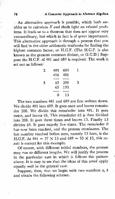
78 A Concrete Approach to Abstract Algebra
An alternative approach is possible, which both en-
ables us to calculate X and sheds light on related prob-
lems. It leads us to a theorem that does not appear very
extraordinary, but which in fact is of great importance.
This alternative approach is through a process that you
will find in the older arithmetic textbooks for finding the
highest common factor, or H.G.F. (The H.G.F. is also
known as the greatest common divisor, or G.G.D.) Sup-
pose the H.G.F. of 481 and 689 is required. The work is
set out as follows:
481 689 1
416 481
65 208 3
65 195
0 13
The two numbers 481 and 689 are first written down.
We divide 481 into 689. It goes once and leaves remain-
der 208. We divide this remainder into 481. It goes
twice, and leaves 65. This remainder 65 is then divided
into 208. It goes three times and leaves 13. Finally 13
divides 65. It goes exactly five times. The remainder 0
has now been reached, and the process terminates. The
last number reached before zero, namely 13 here, is the
H.C.F. As 481 = 37 X 13 and 689 = 53 X 13, this re-
sult is correct for this example.
Of course, with different initial numbers, the process
may run to different lengths. We will justify the process
in the particular case in which it follows the pattern
above. It is easy to see that the ideas of this proof apply
equally well in the general case.
Suppose, then, that we begin with two numbers a, b
and obtain the following scheme.

Finite Arithmetics 79
n a b mnc ma
<1 d c Pqe pd
0 e
This is equivalent to the following equations.
b — ma — c (1)
a — nc = d (2)
c — pd = e (3)
d — qe = 0 (4)
We want to prove that e is the H.C.F. of a and b; that
is, we want to show that a and b are multiples of e,and
that no number larger than e is a factor of both a and b.
From equation (4), d is a multiple of e.
From equation (3), c — pd + e, so c is a multiple of e.
From equation (2), a = nc + d. As c and d are bothmultiples of e, so is a.
From equation (1), b — ma + c. As a and c are mul-tiples of e
,so is b. This establishes that a and b are mul-
tiples of e. Now suppose that some number k is a factor
of both a and b.
Equation (1) shows that k is also a factor of c. As k is afactor of a and c, equation (2) shows that k is a factor of d.
Then equation (3) shows that A; is a factor of e.
Hence any common factor k of a and b is a factor of e.
It is thus impossible that k should be larger than e. Hencee is the H.C.F. of a and b. Q.E.D.We can draw a further consequence from these equa-
tions. In equation (3) we can substitute for d from equa-tion (2). This gives
e = c — p(a — nc) = c( 1 + pn) — pa.
In this equation we can substitute for c from equation (1).

80 A Concrete Approach to Abstract Algebra
e — (1 + pn)(b — ma) — pa—
(1 + pn)b — a(m + pmn + p)-
Thus e has been expressed in the form ax + by where x
and y are integers. It does not disturb us that x happens
to be negative.
The letter h is frequently used for the H.G.F. Using
this notation, we have the important theorem 3.
theorem 3. If h is the H.C.F. of the integers a,
b, there
exist integers x, y such that
h — ax + by.
For example, the numbers 31 and 40 have H.C.F. 1.
Thus it must be possible to find whole numbers x, yfor which
31* + 40y = 1.
To find these by trial and error would not be too easy.
If we carry out the H.C.F. process and apply the argu-
ment used above, we find that x — — 9, y = 7 is a solu-
tion. (Other solutions also exist.)
EXERCISES
1. Find integers x, y to satisfy (i) 3x + 5y = 1, (ii) 8x +13y = 1, (iii) 17x + 12\y
= 1.
2. Could there be integers x, y for which Ax + 6y = 1?
3. What is the necessary and sufficient condition that k must
satisfy if ax + by — k is to have a solution in integers x, y?
a, b are given integers.
We are now in a position to deal with the question of
division in the arithmetic modulo n, with n prime.
If, as before, P and Q stand for the classes to which
given numbers p and q belong, solving PX = Q is equiv-

Finite Arithmetics 81
alent to finding a number x such that px is in class Q.
This means that, for some a,px = na + q. Conversely,
if we can find numbers x, a to satisfy this last equation,
then PX — Q for the class X containing x.
Now n is prime, p is not a multiple of n, for that wouldmean P = O. The only factors of n are 1 and n itself.
Since n is not a factor of p ,the H.C.F. of n and p must
be 1. Accordingly, by Theorem 3, we can find integers
u, v for which pu + nv = 1
.
Multiply this equation by q.
Hence
Let
puq + nvq = q.
Thenx = uq, a — —vq.
px — na = q.
Hence PX = Q as required. Note that, if u belongs to
the class U,
PU = I.
In the modulo n, arithmetic, U is I/P, the reciprocal
of P. Theorem 3 has in effect enabled us to show that
every class P has a reciprocal I/P. If we multiply this
reciprocal by Q, we arrive at Q/P, the desired quotient.
EXERCISES
1. In the arithmetic modulo 17, find the reciprocals of 7and 11.
2. In the arithmetic modulo 257, find the reciprocals of 43and 16.
3. In the arithmetic modulo 11, simplify the fractions 2/7and 5/6.

82 A Concrete Approach to Abstract Algebra
The calculations above are simply intended to help
you to fix the content of theorem 3 in your mind. Need-less to say, it is the light this theorem throws on general
theory that is important, not its use in calculations such
as question 2 above. We rarely need to perform calcula-
tions of this type.
Note that the proof above makes no mention of the
finiteness of the structure. The line of thought here
followed proves fruitful in connection with infinite fields,
as we shall see.

Chapter 4
An Analogy Between Integers
and Polynomials
There are many resemblances between the integers' '
’>
—5, — 4, — 3, — 2, — 1, 0, 1, 2, 3,
• ••
,and the poly-
nomials a, bx + c, dx 2 + ex + /,• •
•,where a
,b, c, d, e,
f, • ••
,stand for rational numbers. Actually, I do not
have to insist on the coefficients a, b, c,,being ra-
tional numbers. They could be chosen from any field
without harming the analogy. I specify the rational field
in order that we may have something definite andfamiliar.
The resemblance will become apparent if you runthrough axioms (7)-(72), and see which of them are
true for our polynomials. If you add two polynomials,
the result is a polynomial. If you multiply two polyno-mials, the result is a polynomial. Thus axioms (7) and(2) hold. Axioms (3) through (7), the familiar laws of
algebra, certainly hold. Axiom (5) holds; subtraction canbe done with polynomials. Axiom (9) holds; when yousubtract a polynomial from itself you get zero. Axiom(70) does not hold. x/(x,+ 1) is not a polynomial. Axiom(77) does hold; 1 is a polynomial. Axiom (72) also holds;
if a product of polynomials is zero, one factor must be

84 A Concrete Approach to Abstract Algebra
zero. Here, of course, “a polynomial is zero” means that
the polynomial is 0 + 0* + Ox2. Axiom (72) amounts to
saying that, when you start out to multiply, say, x — 1
and x + 1 ,neither of which is zero, you can be sure that
the product will not be 0 + Ox + Ox2. The product is,
of course, x2 — 1. You are speaking in quite a different
sense if you say, “But x2 — 1 is zero if x is —1 or 1.” Wewent into this distinction in chapter 2.
The structure formed by the polynomials thus satisfies
all the field axioms except (70). If you will look back to
the chart in chapter 2, you will see that the integers did
exactly the same.
Question: Do the integers and the polynomials con-
stitute isomorphic structures?
Division
In a field, division can be carried through without
remainder. In the structures we are now considering,
that cannot be done owing to the absence of axiom (70).
We can however carry out division in an amended sense.
44 divided by 9 gives 4 with remainder 8.
x 2 divided by x — 1 gives x + 1 with remainder 1
.
How shall we describe what we do when we divide 44
by 9? We might say that we consider the multiples of 9,
and see which of them comes nearest to 44. This suggests
that 45 does, and that we might say 44 divided by 9 gives
5 with remainder — 1 . This might indeed give a simpler
and neater theory of division. We will, for the moment,keep both possibilities in mind. The multiples of 9 are
the numbers 9n. How near 9n is to 44 is estimated byconsidering 44 — 9n. We might make a table.

Analogy Between Integers and Polynomials 85
n 44 — 9n
2 26
3 17
4 8
5 -16 -107 -19
As we go away from n = 4 and n = 5, the numbers in
the second column get numerically larger. +8 and — 1,
we may say, are the simplest numbers in the second
column. It is a matter of opinion whether +8 or —1 is
the simpler. In grade school arithmetic, 8 is definitely
simpler, because it would take us so long to explain whatwe meant by —1. To someone familiar with the integers,
however, —1 might well seem simpler than +8, since
|
—1| is smaller than |8|.
Whichever view we adopt, we can say that the quo-tient is that number for which 44 — 9n is simplest. Theremainder is the corresponding value of 44 — 9n.
By either convention, the remainder is always simpler
than the divisor. By the grade school convention, the
remainder 8 is a simpler number than the divisor 9. Bythe other convention, since
|
—1| < |9|, —1 is simpler
than 9.
This kind of division, then, implies that we have someway of deciding whether one element is simpler thananother.
We know from experience that we can do long division
with polynomials until we reach a remainder of lower
degree than the divisor. Accordingly, we are led to makethe convention that a polynomial /(*) is simpler than a
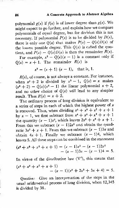
86 A Concrete Approach to Abstract Algebra
polynomial g(x) if fix) is of lower degree than g(x). Wemight expect to go further, and explain how we compare
polynomials of equal degree, but for division this is not
necessary. If polynomial P(x) is to be divided by D{x),
there is only one Q(x) that makes P(x)Q(x)D(x) of
the lowest possible degree. This Q(x) is called the quo-
tient, and P(x) - Q(x)D(x) is then the remainder R(x).
For example, x 2 - Q(x)(x - 1) is a constant only if
Q(x) = x + 1. The remainder R(x) is
*2 - (x + 1) (x - 1), that is, 1.
R(x), of course, is not always a constant. For instance,
when x3 H- 2 is divided by x 21, Q(x) — x makes
(*3 2) — Q(x)(x2 — 1) the linear polynomial x + 2,
and no other choice of Q(x) will lead to any simpler
result. Thus R(x) = x + 2.
The ordinary process of long division is equivalent to
a series of steps in each of which the highest power of x
is removed. Thus, when dividing x4 + x 3 + x 2 + x + 1
by x — 1, we first subtract from x4 + x 3 + x 2 + x + 1
the quantity (x — l)x 3,which leaves 2x3 + x2 + x + 1.
From this we subtract (x - l)2x2 and obtain the quad-
ratic 3x 2 + x + 1. From this we subtract (x — l)3x and
obtain 4x + 1. Finally we subtract (x — 1)4, which
leaves 5. All these steps can be combined in the statement
(x4 + x3 + x 2 + x + 1) ~ (x - l)* 3 ~ (x ~ l)2x 2
— (x — l)3x — (x — 1)4 = 5.
In virtue of the distributive law (V'), this means that
(x4 + x3 + x2 + x + 1)
— (x — l)(x3 + 2x2 + 3x + 4) = 5.
Question: Give an interpretation of the steps in the
usual arithmetical process of long division, when 12,345
is divided by 38
.

Analogy Between Integers and Polynomials 87
Factors
With integers or polynomials, division usually leaves a
remainder. It may however happen, as when 12 is di-
vided by 3, or x 2 — 1 by x — 1, that the remainder is
zero. In this case we say that the divisor is a factor. 3 is a
factor of 12, x — 1 is a factor of x 2 — 1. d is a factor ofpwhen, for some integer q, qd = p. D(x) is a factor of P(x)
when, for some polynomial Q(x), Q(x)D(x) = P(x).
The numbers 1 and —1 are factors of every integer.
For any integer n, n — 1-n — (—
1 )•( — «). This factor-
ization is trivial.
definition. An element that is a factor of every element of
a structure is called a unit.
What are the units in the system of polynomials? Wecan eliminate at once any polynomial of the first or
higher degree. For such a polynomial, P(x), is certainly
not a factor of P(x) + 1 . There remain only the constant
polynomials. Apart from zero, these are factors of every
polynomial. For instance, 2 is a factor of x + 1 since
x + 1 = 2(|x + ^). You will remember that at the out-
set of this chapter we said we should accept as eligible
any polynomial with rational coefficients.
Since any constant non-zero A: is a factor of any poly-
nomial, we also regard these factors as trivial. A teacher,
wishing a class to see that x6 — 1 could be factored as the
difference of squares or as the difference of cubes, might
ask, “Is there any way of starting to factor x6 — 1
other than (x 3 — l)(x 3 + 1)?” A pupil might suggest
(2x3 — 2)(|x 3 + J), and the teacher might say, “Well,
that is really the same factorization, isn’t it?” “Really
the same” means that only a trivial operation has been
performed.
In the same way, a pupil who factors x 2 — 1 as

88 A Concrete Approach to Abstract Algebra
(2x— 2) + |) has undoubtedly given a correct an-
swer. One might point out that (x — 1)(* + 1) is a
somewhat more convenient form of this answer.
A prime element is one that has no factors except trivial
ones. Thus the factorization (— 1)*(— 3) does not pre-
vent 3 from being a prime number. The factorization
2(i* + |) does not prevent x + 1 from being a prime
polynomial.
Note that we call an element prime when it has
no factors within the structure. For example, 3 =
(Vl - 2)(a/7 + 2) and x2 - 2 = (x - V2)(x + V2).
But V7 - 2 and V7 + 2 are not integers, and x — V2and x + V2 are not polynomials with rational coeffi-
cients. 3 and x 2 — 2 are prime elements of the integers
and of polynomials over rationals respectively.
Highest Common Factor
d is a common factor of a and b if a = pd, b — qd,
with p and q elements of the structure.
We now have to explain what we mean by the
“highest” common factor. We are looking, of course,
for an explanation that will hold, not only for the inte-
gers, but for any structure reasonably like the integers.
In chapter 3 we met a procedure for determining the
H.G.F. of two given integers a, b. These integers were
then thought of as being positive, but since the H.C.F.
of 8 and 12 is the same as the H.C.F. of 8 and —12,
this is no real restriction. This procedure led us to a
number h with the following properties:
(i) h is a common factor of a and b.
(ii) h = au + bv for some u, v belonging to the
structure.
(iii) any common factor of a and b is a factor of h.
In property (ii) we say “belonging to the structure”

Analogy Between Integers and Polynomials 89
instead of “which are integers” so that we shall not haveto reword the statements when we proceed to considerstructures other than the integers.
It is evident that property (iii) is a direct consequenceof property (ii). Property (iii) is stated here because it
links on to our experiences in elementary arithmetic,
which statement (ii) does not.
We shall consider only structures in which a procedureanalogous to the H.C.F. calculation of chapter 3 can becarried through. We suppose this structure to satisfy thefield axioms, with the exception of (10). The proof inchapter 3 that h has properties (i)—(iii) depends only onthese axioms.
Question: Check this last statement.
Any element h having properties (i)—(iii) will be calleda H.C.F. Later we shall discuss what is involved in
speaking of the H.C.F.
The H.C.F. process depended on repeated divisions.
The field axioms, with (10) removed, are insufficient toguarantee division. As we saw in our analysis of division,
we need (1) a definition of “u is simpler than v”, (2) theproperty that, given any elements a, b, it is possible tofind an element q such that r = a — qb is simpler than b.
We suppose our structure has a definition (1) andsatisfies requirement (2). This is still not quite enough.The H.C.F. process of chapter 3, in the example thereconsidered, gave the sequence of numbers 689, 481,208, 65, 13, 0. These numbers get steadily smaller(“simpler”). This is no accident. For instance, 65 arises
as remainder for a division by 208. So it is bound to besimpler than 208. The same holds for the other numbersin the sequence. The H.C.F., 13, is the number thatoccurs immediately before zero. Thus, an essential fea-ture of the process is that it must terminate. Otherwise,
90 A Concrete Approach to Abstract Algebra
there is no sense in speaking of the element just before
the end.
We therefore require of our structure (3) that every
sequence of elements, u\, u2, M3, • ••
,for which uT+1 is
simpler than ur,terminates. It is impossible to have an
unending sequence of elements, each simpler than its
predecessor.
Here, of course, it is understood that the sequence has
a first term u\. For the integers one could have an infinite
sequence, • ••
, 5, 4, 3, 2, 1, 0, without a beginning. The
H.C.F. process automatically provides initial elements
a, b. The sequence is bound to have a beginning. We de-
mand that it shall also have an end.
In any structure, then, satisfying the field axioms with
the exception of (10), and requirements (1) through (3)
just listed, we can carry through the H.C.F. process, and
find an element h with properties (i) through (iii).
In particular, the H.C.F. procedure can be carried
out for polynomials over the rationals. We verify re-
quirements (1), (2), (3), as follows.
A polynomial corresponds to a sequence (a, b, c, • ••
,
k, 0, 0, 0,• •
• ) . The complexity of a polynomial is meas-
ured by the number of terms that precede the unbroken
run of zeros.
Thus a quadratic (a, b, c, 0, 0, 0,• • •) where c ^ 0 is
less simple than a linear polynomial (d, e, 0, 0, 0,• • •)
where e ^ 0, and this in turn is less simple than
(/, 0, 0, 0,•
• ) where f 0, and this is less simple than
(0, 0, 0, 0, 0,• •
•)? the polynomial zero. No polynomial
simpler than zero can be found.
If B(x) is any polynomial other than zero, the division
process gives us R(x), of the form A(x) — Q(x)B(x), and
this R(x) is simpler than B(x).
Finally, if V\(x) is any given polynomial, we cannot
find an unending sequence V\(x), V2&), Vz(x), • ••
,with
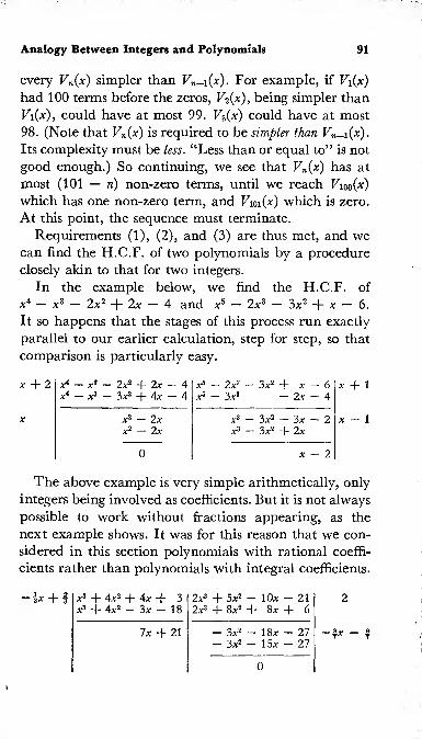
Analogy Between Integers and Polynomials 91
every Vn(x) simpler than Fn_i(x). For example, if V\{x)
had 100 terms before the zeros, V2 (x), being simpler than
V\{x), could have at most 99. V%(x) could have at most
98. (Note that V„(x) is required to be simpler than Vn-i(x).
Its complexity must be less. “Less than or equal to” is not
good enough.) So continuing, we see that Vn(x) has at
most (101 — n) non-zero terms, until we reach Fioo(*)
which has one non-zero term, and Vm(x) which is zero.
At this point, the sequence must terminate.
Requirements (1), (2), and (3) are thus met, and wecan find the H.G.F. of two polynomials by a procedure
closely akin to that for two integers.
In the example below, we find the H.C.F. of
x4 — x 3 — 2x 2 + 2x — 4 and x5 — 2x 3 — 3x2 + x — 6.
It so happens that the stages of this process run exactly
parallel to our earlier calculation, step for step, so that
comparison is particularly easy.
X + 2 x* — x3 — 2x2 + 2x — 4 Xs — 2x3 — 3x2 + x — 6
x4 — x3 — 3X2 + 4x — 4 x8 — 3x3 — 2x — 4
X x2 — 2x x3 - 3x2 + 3x - 2x2 — 2x x3 - 3x2 + 2x
0 x - 2
The above example is very simple arithmetically, only
integers being involved as coefficients. But it is not always
possible to work without fractions appearing, as the
next example shows. It was for this reason that we con-
sidered in this section polynomials with rational coeffi-
cients rather than polynomials with integral coefficients.
i* + ! X3 + 4x2 + 4x + 3 2x3 + 5x2 - lOx - 21x3 + 4x2 — 3x — 18 2x3 + 8x2 + 8x + 6
7x + 21 - 3x2 - 18x - 27- 3x2 - 15x - 27
0

92 A Concrete Approach to Abstract Algebra
This calculation gives the H.C.F. as lx + 21. As this
is 7(x + 3), we may remove the “unit” 7, and take x + 3
as a correct answer. In fact,
x3 + 4x2 + 4x 4* 3 = (* + 3)(x2 + x + 1),
2*3 + 5*2 _ 10* _ 21 = (x + 3)(2x 2 - x - 7).
We have now shown an analogy between integers and
polynomials in regard to division, factors, primes, units,
H.C.F. For we have explained all of these things in gen-
eral terms that apply equally well to the two structures
and, no doubt, to other structures also.
There remains one last point to clear up. How manyelements h can satisfy the conditions?
(i) A is a common factor of a and b.
(ii) h — au + bv for some u, v of the structure.
(iii) Any common factor of a, b is a factor of h.
Suppose that h and k both satisfy these. Then, in virtue
of (i), A; is a common factor of a and b. By (iii), k must be
a factor of h. .*. h — ek for some e. Similarly, by inter-
changing the roles of h and k, k — fh for some /. Henceh = ek = efh. Therefore h{1 — ef) = 0. h is not zero, so,
by axiom (72), 1 — ef = 0. Hence ef — 1. If m is any
element of the structure, efm = m. That is, e and / are
factors of every element of the structure. Accordingly, e
and / are units.
For the integers this means that for a = 12,£ = 18,
the conditions (i) through (iii) are satisfied by 6 and — 6
and by no other numbers.
For the polynomials, if A(x) = (x — 1)(* + 1) and
B(x) — (x ~ 1)(* + 2), then the conditions for H(x)
are satisfied by C(x — 1) for any constant C, and by no
other polynomials.
This degree of uncertainty causes us no trouble. Wehave already seen that multiplication by a unit is a
trivial change. If we know that numbers a and b both

Analogy Between Integers and Polynomials 93
divide by 6, then we know that they both divide by — 6.
It is quite easy to show that if h satisfies properties (i)-
(iii), so does hf, where/is a unit. This degree of vagueness
in the answer is therefore unavoidable. And we proved
that this is all the vagueness there is. We did this whenwe showed that any k satisfying properties (i)-(iii) mustbe of the form hf.
We can, if we like, make a convention to fix h. For
numbers we can say that h must be positive; we choose 6,
rather than —6, for the H.C.F. of ±12 and ±18. For
polynomials, we can require the coefficient of the highest
power of a; to be 1
.
We shall exploit the analogy between integers andpolynomials in the next chapter.

Chapter 5
An Application of the Analogy
We have met two procedures for obtaining a newstructure from an old one.
First, given any field F, we have shown how to con-
struct polynomials over that field. That is, given a field F,
we show that it is always permissible to introduce a newsymbol x and to assume that polynomials a + bx +cx2 + • •
• + kxn,where a, b, c, • •
•,k are elements of F,
satisfy the commutative, associative, and distributive
laws.
Second, given a structure such as the integers, we obtain
a field from it in the following way. We select a prime
element, p ,of the structure, and we break the structure
up into classes. Two elements belong to the same class
if they leave the same remainder on division by p. If
element a belongs to class A and element b to class B
,
then A + B means the class containing a + b, and ABthe class containing ab. By a structure “such as the
integers,” we understand one in which all the field ax-
ioms except (70) apply, and also the three conditions
listed in chapter 4 that make the H.C.F. process possible.
We then know that the classes A, B, • ••
,form a field, for
our proofs in chapters 3 and 4 used only the field axioms
and the three conditions.

An Application of the Analogy 95
Both procedures we have a right to carry out. We donot need to have any doubts whether what we are doing
is justified. We spent a good deal of time in chapter 2
showing that a new symbol x could always be brought
in : it expressed merely the properties of sequences
(a, b, c, • ••
,k, 0, 0, 0, • * •) formed from the elements of
the field F. That is, it expressed the properties of some-thing already there: it did not really bring in anything
new. In the same way, the second procedure dealt with
classes of elements in the structure. It, too, involved nonew assumption.
It will be convenient to have names for these proce-
dures, so that we can refer to them without a long ex-
planation. The first procedure we will call adjoining an
indeterminate x to the field F. In the second procedure, froma suitable structure S, we form the residue classes modulo p.
Thus, the arithmetic of Even and Odd is the structure
formed from the integers by considering the residue
classes modulo 2. “Residue” is a word more or less
synonymous with “remainder”; for some reason, it has
become customary to use it in this connection.
Having these two procedures, we naturally look for
structures to apply them to: in this way, we hope for a
good crop of new structures.
The first procedure we have already applied to quite
a number of fields: we have considered polynomials
with real coefficients, polynomials with rational coeffi-
cients, polynomials with coefficients O, I, II, III, IVfrom the arithmetic modulo 5, and polynomials with
coefficients from the other modular arithmetics. It is also
possible to adjoin an indeterminate x to a structure that
is not a field, as when we consider polynomials with
integers as coefficients: the integers do not form a field.
This however we have not investigated yet.
It does not look as though the first process is likely to

96 A Concrete Approach to Abstract Algebra
open new horizons for us. We have already used it quite
often; it has not led to any particularly novel idea.
How about the second process? So far, we have applied
it to one structure only—the integers, from which wehave obtained finite fields: the arithmetic of Even andOdd, the arithmetics modulo 3, modulo 5, modulo 7,
and so on. To what else can we apply it? There is anobvious candidate. In chapter 4 we saw that polynomials
resembled the integers very closely. The natural structure
to consider is that of polynomials. This still leaves us
some choice; we might consider polynomials with real
coefficients, or rational coefficients, or coefficients fromone of the modular arithmetics.
Suppose we pick polynomials with real coefficients.
When we obtained the arithmetic modulo 5 from the
integers, our first step was to choose the prime number 5.
Here, our first step must be to choose a prime poly-
nomial—one that cannot be factored, x2 + 1 is such a
polynomial. For suppose it had a factor. This factor
would have to be linear, say bx — c. Taking out the con-
stant factor b, we can reduce bx — c to the form x — a.
By the remainder theorem, x — a is a factor of a poly-
nomial /(*) if and only if f(a) = 0. So x — a is a factor
of x2 + 1 only if a,2 + 1 is zero. But, for any real number
a, a2 + 1 is larger than 1, hence not zero. So x2 + 1 has
no factors within the set of polynomials with real coeffi-
cients. It is a prime polynomial. (In books on algebra
the word “irreducible” is usually employed instead of
“prime.” The meaning is the same.)
Accordingly, if we begin with polynomials over the
real numbers and form the residue classes modulo(x2 -f- 1), we are bound to arrive at a field.
When we constructed the arithmetic modulo 5, weonly needed the symbols O, I, II, III, IV because divi-
sion by 5 could only give the remainders 0, 1, 2, 3, 4.

An Application of the Analogy 97
Division by a2 + 1 will never give as a remainder any-
thing more complicated than a linear polynomial, ax + b.
These remainders serve to label the various classes; one
class consists of all the polynomials that leave remainder
4a: — 1, and so on. A remainder may of course be con-
stant. Thus 4a:2 + 6 leaves remainder 2.
We introduce the following notation."
Let 1 stand for the class of polynomials that leave remainder 1
.
Let 2 stand for the class of polynomials that leave remainder 2.
Let 3 stand for the class of polynomials that leave remainder 3.
Let k stand for the class of polyno mials that leave remainder k.
Let J stand for the class of polynomials that leave remainder x.
This notation will prove sufficient for our needs.
Since * belongs to the class J, and 3 belongs to the
class 3,3J is the class containing 3a.
Since 3a: belongs to the class 3J, and 2 belongs to the
class 2, 3J + 2 is the class containing 3x + 2.
In the same way, quite generally, aj + b is the class
containing ax + b.
We could now, ifwe liked, work out sums and products
directly from the definition.
For example, to find (2J + 3)(4J + 5), we could rea-
son that 2J + 3 is the class containing 2a: + 3, and
4J + 5 is the class containing 4a + 5. So(2J + 3)(4J + 5)
is the class containing (2a + 3) (4a + 5). (2a + 3) (4a + 5)
= 8a2 + 22a +15, which, on division by a2 + 1, leaves
22a + 7. The class containing 22a + 7 is 22J + 7.
Hence
(2J + 3)(4J + 5) = 22J + 7.
But it is not really necessary to go through all this.
For we know that the residue classes constitute a field.
Accordingly, they obey the ordinary laws of algebra.
So we may multiply out i
(2J + 3)(4J + 5) = 8J! + 22J + 15.
;
Two points arise here. First, are we entitled to as- -
1

98 A Concrete Approach to Abstract Algebra
sume that 2-4 = 8? Is it correct to multiply the bold-
face numbers just as if they were ordinary numbers?Second what is J
2?
The first question asks us to justify what we have
already done. The second points to still unexplored
territory.
The first point is soon dealt with; it does require us
to go back to the definition, but as the result is a general
rule, we are saved the bother of appealing to the defi-
nition each time. 2 is the class containing 2, 4 is the class
containing 4. By definition 2-4 is the class containing
2-4, which is 8. The class containing 8 is called 8.
So 2*4 = 8.
The argument here used applies equally well to addi-
tion; it does not in any way depend on the particular
choice of the numbers 2 and 4. We conclude that the
boldface numbers can be added and multiplied by the
ordinary processes of arithmetic. We do not have to
learn any new tables. In technical language, the ele-
ments k are isomorphic to the numbers k.
We now come to the second point: what is J2? Here
again, we go back to the definition of multiplication for
residue classes. J is the class to which x belongs, so J •Jis the class to which x-x belongs. That is, J
2is the class
containing x2. But when x2
is divided by x2 + 1 the
remainder is —1. Hence J2 = —1.
We thus reach a striking conclusion. The elements
aJ + b can be added and multiplied by the ordinary
rules of arithmetic and algebra together with the equa-
tion
J2 = -I-
We have, in effect, arrived at a theory of complex
numbers. J does what we expect the square root of
minus one to do.
Let us look back at what we have done. We began

An Application of the Analogy 99
with the field of real numbers. We applied two proce-
dures to it, that we knew were permissible and wouldlead to a field. We obtained a field, containing elements
a, that behaved exactly like the original real numbers a,
and also containing an element J for which J2 = — 1.
Since the elements a have exactly the same pattern
as the numbers a,no harm will be done if we now forget
the distinction between a and a. We can then say simply
that to the real numbers a we adjoin a new element Jfor which J
2 = — 1 . The structure so obtained is a field
:
that is to say, our algebraic habits do not have to be
changed when we are working with it.
If you feel that there is something unfair in identifying
a with a, it is quite possible to maintain the distinction
between a and a and yet get information about the real
numbers. We shall illustrate this by deriving a partic-
ular identity, of some mathematical and historical inter-
est.
First of all, (a + bj)(a - bj) = a2 - b2J
2 = a2 + b2.
Similarly, (c + dj) (c — dj) = c2 + d2. Accordingly,
(a2 + b2)(c2 + d2)
= (a + bj)(a - bj)(c + dj)(c - dj)
= (a + bj) (c - dj)(a - bj)(c + dj)
= {ac + bd + J(bc — ad)} (ac + bd — J(bc — ad)}
= (ac + bd) 2 - J2 (bc - ad) 2
= (ac 4~ bd) 2 + (be — ad) 2.
But we showed earlier that the elements a, b, c, dcombined with each other in exactly the same way as
the numbers a,
b, c, d. In view of this isomorphism, wededuce that, for any real numbers a, b, c, d,
(a2 + b 2) {c
2 + d2) = {ac + bd) 2 + {be - ad)2
.
This result is of some interest in the theory of numbers.
Any whole number can be expressed as the sum of four
squares. Thus, 7 = 4 + 1 + 1 + 1 = 2 2 + l2 + l
2 + l2
.

100 A Concrete Approach to Abstract Algebra
Thus it is easily seen that 7 cannot be expressed as
the sum of fewer than four squares; 1 and 4 are the only
squares small enough to be used. It is thus a definite
property of a whole number if it can be obtained by
adding less than four squares together. For example, 13
is 9 + 4, the sum of two squares. 17, being 16 -f- 1, is
also the sum of two squares. The identity above tells us
that, when two such numbers are multiplied together,
their product also is the sum of two squares. 13 X 17 is
221. If we put a = 2, b = 3, c = 4, d = 1 in the identity
we get
13-17 = ll 2 + 102,
and this expresses 221 as the sum of two squares.
The identity also has some relation to trigonometry.
This identity could, of course, be proved by means of
elementary algebra without bringing J in at all. This
must be so, for otherwise we should have got a result
by using J that was not true for the algebra without J.
But the whole point of our earlier work was to show that
the presence of J did not make any logical difference
:
given the possibility of the algebra without J, the possi-
bility of the algebra with J was a logical consequence.
Thus the introduction of J cannot lead to any extra
results. We do not want it to; extra results would be
wrong results. It can, however, lead to more convenient
ways of obtaining known results. It can simplify proofs
and illuminate theories. If you are sufficiently familiar
with complex numbers, the proof of the identity given
above is a natural one. It follows a train of thought that
could lead you to the identity if you did not already
know it.*
In trigonometry it is well known that many results
can be obtained far more quickly and easily by using
* Ifw = a + bJ, z = c — dJ, the identity, in modulus notation,
states |w| • |z| = \wz\.
An Application of the Analogy 101
\/—l than by any other method. As the trigonometrical
functions belong to analysis rather than to algebra (they
require infinite processes for their definition), we shall
not discuss them here. They are mentioned only as
showing that the right to introduce V/— 1 is a valuable
one.
For the present, it will be sufficient to consider our
demonstration of the algebraic identity above. Someone
might say that this particular result could be proved
just as easily by elementary algebra. We are not con-
cerned with this criticism. \/— 1 has proved itself very
fruitful in many branches of mathematics; its claim to
usefulness is not based solely on this particular identity.
We are defending not the usefulness but the correctness
of our method. Our proof may not be the neatest proof;
but is it a proof at all?
“No,” says our critic, “of course it isn’t. You have a
symbol J and you write J2 — — 1. Well, that just is
not so. You can’t find a number J such that J2 = —1.”
The interesting thing about this argument is that
everything, except the conclusion, is correct. We do have
a symbol J and we do write J2 = — 1. It is also true that
no number has its square equal to — 1.
Our critic’s mistake is in supposing that these true
statements in any way detract from our proof of the
identity. They do not. We have at no point said that J repre-
sented a number. All we assumed, in the various steps wetook, was that J obeyed the ordinary laws of algebra. Our“
critic’s assumption (probably based on something his
teacher told him, authoritatively, and without any evi-
dence to back it up) is that algebraic symbols always
represent numbers.It may help to summarize the rather lengthy process
we have been through, if we present our argument in the
form of a discussion with the critic.

102 A Concrete Approach to Abstract Algebra
Ourselves. I understand that you feel quite happy with
calculations that only use real numbers, such as 2, — 3,
3/4, V2, tt?
Critic. Yes.
Ourselves. And you are then quite happy with poly-
nomials such as 2x — 3 or x2 + 2, and you are able
to calculate with these?
Critic. Yes.
Ourselves. In particular, you admit that it is possible to
divide such polynomials by x2 + 1 and see what re-
mainder results.
Critic. Yes, of course.
Ourselves. So that, for instance, x3 + x + 2 and 3x2 + 5,
on division by x2 + 1, both leave the remainder 2?
Critic. That is correct.
Ourselves. And there would be nothing vicious then in
saying that all polynomials with this property could
have the label 2 attached to them?
Critic. No. I cannot object to that.
Ourselves. And we could attach the label J to any poly-
nomial that left remainder x, and the label — 1 to any
polynomial that left remainder —1?
Critic. Certainly.
Ourselves. Would there be any objection to recording
in the form 2-x = (2x) the fact that when any poly-
nomial labeled 2 is multiplied by any polynomial
labeled x the product is always to be labeled 2x?
Critic. No. That is simply a notation, and does not
commit me to any new admission.
Ourselves. And, similarly, we could explain the nota-
tion 2 + x?
Critic. Yes.
Ourselves. And we could then check that all the labels
aJ + b, together with the signs + and •,obeyed the
axioms (7) through (72) for a field?

An Application of the Analogy 103
Critic. I am willing to accept your word that anyone
who did not find it too boring could do so.
Ourselves. And by means of these axioms we could
justify all the steps taken with the symbols a, b, c, d, Jin our demonstration of the identity?
Critic (after some thought). Yes; you have only handled
these symbols in accordance with the rules allowed byaxioms (7) through (72).
Ourselves. And finally we arrived at a result,
(a2 + b2)(c2 + d2) = (ac + bd)
2 + (be — ad) 2,
in which J does not appear?
Critic. Yes.
Ourselves. But we also noticed that there was a very
close resemblance between operations on the classes
a, b, c, d and calculations with the corresponding
numbers, a, b, c, d. For instance, can you find anyexample where a + b = p but a + b is not p? Orone where a • b = q and a • b is not q?
Critic (after trying a few examples, and making somealgebraic calculations). No, there are no such cases.
Ourselves. And also if a — b = r, then it must be that
a — b — r?
Critic. Yes, certainly.
Ourselves. Our algebraic identity is built up by a chain
of additions, subtractions, and multiplications?
Critic. Yes.
Ourselves. So the corresponding identity must hold for
a, b, c, d
?
Critic. Yes, it seems so.
Ourselves. In that case, we have proved our identity
with the help of the symbol J, which does not repre-
sent a number. And you have admitted the logic of
our procedure.
Critic. I feel I am being cheated, but I cannot say just
where.

104 A Concrete Approach to Abstract Algebra
The idea of V—1 is still new enough for us to feel
that it is strange. But in past centuries, it felt equally
strange when the number "s/2 had to be brought in to
describe the ratio between the lengths of the diagonal
and the side of a square. Before that time, only rational
numbers, p/q, withp and q integers, had been considered.
It was proved by the ancient Greeks that there cannot
be a rational number * for which x2 = 2. For if there
were, this number could be expressed as p/q where p
and q have no common factor (since any common factor
could be canceled). In particular, we may assume that
p and q are not both even: if they were both even, we
could keep on canceling 2 until an odd numerator or
denominator appeared. We suppose all possible canceling
has been done, and that (p/q)2 = 2; that is, p
2 = 2
q
2.
The square of an odd number is odd. But p2,being 2q
2,
is even. Hence p cannot be odd. So p must be even.
Hence q must be odd, as all possible canceling has been
done. But, as p is even, we can write p — 2k. Then
jb2 — 2
q
2 shows that Ak2 — 2q2 or q
2 = 2k2. But q is odd,
so q2
is odd. 2k2is even.
We have arrived at the conclusion that an odd number
equals an even one. This is a contradiction. So there
must have been something wrong with the assumption
made at the outset, that x2 — 2 could have a rational
solution. Since this assumption leads to an absurdity, it
must be false.
So an ancient Greek, who thought of numbers as con-
sisting only of rational numbers, 3§, f, 5|, and so on,
could have said, “No number has square equal to 2,”
with just as much conviction as our critic who said,
“No number has square —1.”
Our procedure is equally suitable for convincing him.
We begin with the field of rationals, which he admits.

An Application of the Analogy 105
(An ancient Greek would not have recognized negative
numbers. We suppose this difficulty to have been over-
come first.) We adjoin to this an indeterminate *, andthus obtain polynomials with rational coefficients. Wethen select the prime polynomial x2 — 2. This is primeover the rationals, for if it had a factor x — a with a
rational, then a2 — 2 would be zero, and there is norational number for which this happens. So, when weclassify polynomials with rational coefficients in accord-
ance with their remainders on division by x2 — 2 (in
other words, when we form the residue classes modulox2 — 2), we obtain a field.
Once again, we introduce a notation.
1 is the label for any polynomial leaving remainder 1.
2 is the label for any polynomial leaving remainder 2.
K is the label for any polynomial leaving remainder x.
Then K2 or K • K, is the label for the class containing
x2. But x2
,on division by x2 —
2, leaves remainder 2.
So the class K2is the class 2.
K2 = 2
As division by x2 — 2 leaves a linear remainder a + bx,
all our labels are of the type
a + bK.
We can prove results for rational numbers with the
help of K, just as we proved results for real numberswith the help of J. The steps of the following argumentrun exactly parallel to the steps used earlier to establish
an identity about the sums of squares.
(a + bK)(a - bK) = a2 - b2K2 = a2 - 2b2.
Similarly,
(c + dK)(c - dK) = c2 - 2d2.
Accordingly,

106 A Concrete Approach to Abstract Algebra
(a2 - 2b 2) (c
2 - 2d2)
= (a + bK) (a - bK)(c + dK)(c - dK)
= (a + bK) (c - dK) (a - bK)(c + dK)
= {ac - 2bd + K(bc - ad)}
{ac — 2bd — K(bc — ad)}
= (ac - 2bd)2 - K2(bc - ad) 2
= (ac - 2bd) 2 - 2 (be - ad) 2.
As before, there is an isomorphism relating a, b, c, d,
to a, b, c, d,and we have, for rational numbers a
,b, c, d,
the relationship
(a2 - 2b2) (c
2 - 2d2) = (ac
- 2bd) 2 -2 {be - ad) 2.
Once the logical correctness of introducing K with
K2 = 2 has been admitted, we may use the sign V2instead of K; and finally, in view of the isomorphism
between the classes a and the numbers a,we may drop
the boldface. We thus reach our usual notation a + bV2.
EXERCISES
1. Show that, over the arithmetic modulo 3, the poly-
nomial x2 + 1 is prime (irreducible). Can a theory of complex
numbers be constructed for the arithmetic modulo 3? Investi-
gate and discuss.
2. Show that x2 + 3 is an irreducible (that is, nonfactor-
able) polynomial over the arithmetic modulo 5. Is x2 + 1 irre-
ducible over the arithmetic modulo 5? Is a field obtained by
applying the usual rules of arithmetic and algebra (i) to the
elements a + bV— 1,
(ii) to the elements a + bV— 3? a, b
stand for the elements 0, 1, 2, 3, 4 (or O, I, II, HI, IV, if
you like) of the arithmetic modulo 5.
3. In the arithmetic modulo 2 it is possible to write down
all the factorable quadratics, by listing all the expressions

All Application of the Analogy 107
(x -f- a)(x + b) and multiplying them out. Do this. Is there
any irreducible quadratic x2 + px + q over this arithmetic?
If so, how many such quadratics are there?
4. Consider the residue classes, modulo x2 + x + 1, of
polynomials over the arithmetic modulo 2. Let 0 label the
polynomials giving remainder 0, 1 label the polynomials giv-
ing remainder 1, M label the polynomials giving remainder x.
Fill in the spaces of the multiplication table below.
0 1 M M + 1
0
1
MM + 1
5. In question 4, let “modulo x2 + x + 1” be replaced by
“modulo x2 + 1,” the question otherwise remaining unaltered.
Answer this amended question : Do the residue classes, modulo
x2-f- 1, of polynomials over the arithmetic modulo 2, form a
field? If not, which axioms fail?
6. Do the elements 0, 1, M, M + 1 of question 4 form a
field?
7. Consider the residue classes, modulo x2,of polynomials
over the real numbers. Let Q label the class of polynomials
that leave remainder x, K the class that leave remainder k,
for any constant k. Find the product (2 + 3Q) • (4 + 5Q).Do the elements a + bQ, form a field?
8. Show that the H.C.F. procedure applied to a + bx andx2 + 1 enables us to find a linear polynomial f(x) and a con-
stant k such that 1 = (a + bx)f(x) + (x2 + \)k. Find the poly-
nomial f(x) and deduce the reciprocal of a + bj where
J2 - -1.
9. What field results from considering the residue classes
modulo x of polynomials over the reals? If f(x) and g(x) are
two polynomials belonging to the same residue class modulo x,
what can be said about the graphs of y = fix) and y = g(x)?
10.
Determine the equation whose roots are the elements
0, 1, M, M + 1 of question 4.

108 A Concrete Approach to Abstract Algebra
Must We Distinguish Between 1 and 1?
This is a point that troubles some students. In the
ordinary course of development, we begin with numbers
0, 1, 2, 3,• •
•,as used in counting, the natural numbers.
We then meet fractions, which we think of as lying be-
tween the natural numbers; If, If, If and many others
lie between 1 and 2.
Then perhaps we meet negative numbers, —1, —If,
— If, —If, —2, • ••
,which we may think of as lying to
the left of zero.
With the Pythagorean Theorem we meet s/2, which
lies between If and 1^; from the circle we meet tt,
which lies between 3 and 3f. These are irrational num-
bers.
Rational and irrational numbers together make up the
real numbers. Then we go beyond these to consider
complex numbers, x + jyV— 1. If y happens to be zero,
the complex number reduces to a real number. We think
of 4 + oV— 1 as being simply the real number 4.
Thus real numbers are thought of as being part of the
complex numbers; rational numbers as part of real
numbers; integers as part of rationals; the natural num-
bers as part of the integers. All this we think while in a
state of innocence.
Then we meet a mathematical philosopher who points
out that, in order to justify the use of V :2, we had to bring
in a symbol K, a label for any polynomial that left
remainder x on division by x2 — 2. K thus stood for a
collection of polynomials. In the same way 2 stood for
a collection of polynomials—all those that leave re-
mainder 2 on division by x2 — 2. Then we had K.2 = 2.
Now, says the philosopher, the number 2 is a very differ-
ent thing from 2, a collection of polynomials. Admittedly

An Application of the Analogy 109
there is an isomorphism, 2 + 3 = 5 corresponding to
2 + 3 = 5. But 2 and 2 are different things, and youmust not forget this.
Now this matter is somewhat crucial, for an argumentof this kind arises at each step in the extension of number.In passing from whole numbers to fractions, a philosoph-
ical theory considers number pairs (p , q) which eventually
turn out to play the role of p/q. Now a number pair is
not the same thing as a number, so (says the philosopher)
we must distinguish between the natural number 4 andthe fraction (4, 1) or 4/1.
Negative numbers also can be introduced by numberpairing. Thus +4 corresponds to any pair such as (7, 3)
in which the first number is 4 more than the second, — 4to any pair such as (5, 9) in which the first number is
4 less than the second. Thus the philosopher distinguishes
between the natural number 4 and the positive inte-
ger +4.In the same way a distinction is drawn between the
integer +4 and the real number 4, and between the real
number 4 and the number 4 + 0V— 1 occurring in
complex number theory.
Thus, according to this philosopher, the real numbersdo not form part of the complex, nor the rationals of the
reals, nor the integers of the rationals, nor the natural
numbers of the integers.
How are we to decide what value to attach to such
philosophical arguments? The correct procedure is, I
think, indicated in a passage of a well-known children’s
book.
The first person he met was Rabbit.
“Hallo, Rabbit,” he said, “is that you?”
“Let’s pretend it isn’t,” said Rabbit, “and see
what happens.”
Winnie-the-Pooh

110 A Concrete Approach to Abstract Algebra
Rabbit here seems to be taking a thoroughly scientific
position. Let us apply his approach to the point at issue.
Suppose you cling to the viewpoint of innocence, that
the natural numbers, the integers, the rationals, the
reals, the complex numbers are like a set of boxes, each
contained in the following one. To what errors will this
supposition lead you? So far as I can see, it will not lead
you to any.
Nor, on the other hand, do I see that the philosopher
who insists that +4 is different from 4 is necessarily
going to be led into any particular error. The whole
question seems to be about ways of looking at things,
rather than about any point of fact. We often have
difficulty in saying whether or not two things are “the
same.” Is the man of seventy the same person as the
boy who used to attend the village school? In one sense,
yes; in another sense, no.
This difficulty is particularly acute when we are talk-
ing about abstract ideas, when we are trying to decide
whether the natural number 4 is the same as the fraction
4/1 or different.
Suppose you say, “The conductor stopped the band
after it had played four bars.” Which “four” are you
using there? Since you can count the four bars, it would
be reasonable to answer, “The natural number four, the
four we use when we count 1, 2, 3, 4.” But suppose the
conductor had intervened a little later, when the band
had played four and one-half bars. A\ is clearly a frac-
tion, a rational number. This suggests that the 4 in “four
bars” could be regarded as a rational number equally
well. My own feeling is that it does not matter which
you call it, that the distinction between natural number,
positive integer, rational number, real number, cannot
be maintained in such situations—in fact, that there is
a lot to be said for the viewpoint of innocence. It would
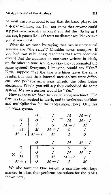
An Application of the Analogy 111
be most unconventional to say that the band played for
4 + OV^— 1 bars, but I do not know that anyone could
say you were actually wrong if you did this. So far as I
can see, it passes Rabbit’s test: no disaster would overtake
you if you did it.
What do we mean by saying that two mathematical
systems are “the same”? Consider some examples. If
you had two calculating machines that were identical
except that the numbers on one were written in black,
on the other in blue, would you say they represented the
same system? Everyone, I imagine, would say “Yes.”Next, suppose that the two machines gave the sameresults, but that their internal mechanisms were differ-
ent—one perhaps using gear wheels, the other being
electronic. Would you still say they embodied the samesystem? My own answer would be “Yes.”
Now suppose we have two calculating machines. Thefirst has keys marked in black, and it carries out addition
and multiplication for the tables shown here. Call this
the black system.
O
M + I
O I M M + I
0 I M M + I
1 0 M + I MM M + I O I
M + I M I 0
O
M + I
0 1 M M + IOOOOO I M M + I
0 M M + I I
0 M + I I MWe also have the blue system, a machine with keys
marked in blue, that performs operations for the tables
shown here,

112 A Concrete Approach to Abstract Algebra
C>
01
I
To
oo"
o
i
01
You will notice that the top left-hand corners of the
“black” tables are the same as the “blue” tables. Shall
we say then that the blue system is a part of the black
system? If we accept the earlier contention, that differ-
ences of color and of internal mechanism are unim-
portant, we are bound to answer “Yes.” The blue ma-
chine is not, of course, part of the black machine, but
the mathematical system represented by, or embodied
in, the blue machine is part of the mathematical system
represented by the black machine.
Now the blue system is, of course, the arithmetic
modulo 2, and the black system is the field obtained
from that arithmetic (as in question 4, p. 107) by con-
sidering residue classes for the irreducible polynomial
AT2
-f- AT + 1-
Our philosopher arrived at these systems in that
order. He first had the blue O and I standing for Even
and Odd. Then he brought in the black 0 as a label for
any polynomial over the arithmetic modulo 2 that hap-
pened to be exactly divisible by x2 + x + 1 (which you
can write lx2 + /* + /, with blue Z’s, if you like). The
black /, the black M, and the black M + I were given
similar meanings.
Having arrived at the black system in this way, our
philosopher cannot get it out of his head that the black O
has a different meaning from the blue 0 . He maintainsi
that the blue system is not a part of the black system,
because of this difference of meaning.
Now we are grateful to him for pointing out that the
black system can be derived, built up, from the blue
system. That is a most helpful observation, and we shall
often make use of it. But because this is “a” way of doing

An Application of the Analogy 113
things, it does not follow that it is “the” only way of
doing things. In mathematics, it very often happens that
a complicated structure is discovered before a simple
one. The black system might have been discovered be-
fore the blue one. Then, we should have discussed it in
its own right. We should have checked to see that it
satisfied all the axioms for a field. We could do all thi s
without mentioning the blue system, without even beingaware that the blue system was possible at all. Thensomeone might have noticed that the northwest corners
of the black tables already constituted a closed system,
a field, with elements O and I. The blue system wouldthen have been discovered, and thought of, as a part of
the black system.
In the same way, we arrived at the complex numbersearlier in this chapter by considering the residue classes
modulo x2-f- 1. This is one way of obtaining the com-
plex numbers, but there are others. One can derive
p + q\Z~ 1 by considering the number pair (p, q) ;in an-
other treatment, “s/— 1 is related to rotation through aright angle; in yet another, matrix theory is used. Wedo not regard these as different complex number systems,
but rather as different ways of realizing one and the
same pattern. It is a waste of time to argue whether y/
—
1
“really is” a residue class of polynomials, or the numberpair (0, 1), or a rotation through 90°, or a particular
matrix.
I do not believe that any mathematical result at all
comes from the discussion in the last few pages. I haveincluded this discussion for two reasons. First, we nat-
urally feel that something questionable is being donewhen we “identify” 1, standing for a collection of poly-
nomials, with the number 1. Second, students pick upwisps and echoes of the philosophical discussions, onwhether the integer 4 and the rational number 4/1 are

114 A Concrete Approach to Abstract Algebra
the same or different, and are bothered by these. Of one
thing I am certain: it is a mistake to lose any sleep over
such matters. The question is psychological rather than
philosophical or scientific. You should feel perfectly free
to adopt whichever answer allows you to work most
happily: indeed, if it suits you, you can adopt now one
view, now the other, according to the problem you are
working on.

Chapter 6
Extending Fields
In CHAPTER5we considered a way of extending a given
field. The method used the idea of residue classes, but,
as we saw in a lengthy discussion, it was often incon-
venient to keep the final result in terms of residue classes.
The residue classes gave us a way of showing that a
certain type of calculating machine could be built, and
indeed of building it. However, once having obtained the
new machine, we shall often want simply to work it,
and to forget what is inside it. So let us look at the fields
we obtain by the procedure of chapter 5, and see just
what this procedure does for us.
At the beginning of chapter 5, by considering residue
classes modulo (x2 + 1), we obtained the symbols a + bJ
where a and b are real numbers and J satisfies the equa-
tion J2 = —1. a bJ is commonly referred to as a
“complex number.” In order to work correctly with
complex numbers, all you need to know is (i) that
complex numbers obey the laws of algebra, (ii) that
J2 = — 1 . Statement (i) here could be put, that complex
numbers form a field. As the real numbers form a field,
in passing from real numbers to complex numbers, weare not conscious of any change, so far as statement (i)
goes. The main novelty lies in statement (ii), that
J2 — —1. So long as we are working with the real

116 A Concrete Approach to Abstract Algebra
numbers, the equation x2 + 1 =0 has no solution. Theeffect of passing to the complex numbers is to bring in a
new symbol J, such that J2 + 1 =0. We thus, so to
speak, create a root for the equation x2 + 1 = 0. Youwill notice that the procedure of chapter 5 used residue
classes modulo (x2 + 1).
In the same way, toward the end of chapter 5, to
obtain a field in which x2 — 2 = 0 had a root, we con-
sidered residue classes modulo (x2 — 2).
Quite generally, if f(x) is an irreducible polynomial
over a field F, we can obtain a field in which the equa-
tion f(x) = 0 has a root by considering residue classes
modulo /(*).
(You should be able to prove this result, by observing
the proofs on pages 98 and 105, for J2 + 1 =0 and
K2 — 2 = 0, and noting that the method used in these
two particular proofs can be used in general. A proof
will be given shortly, but it does no more than carry
out the hint here given : if you can find the proof unaided,
you will gain in insight and confidence.)
In speaking above of statements (i) and (ii) as em-
bodying all you need to know to calculate with complex
numbers, I should perhaps have added something you
need to know is not so. A student might write 2J — 3 = 0,
and say “Why not? How do you know this is not so?”
In this particular case, it is easy enough to show that
this equation is wrong. If 2J — 3 = 0, J = 1§, so
J2 — — 1 would mean (1|)2 = — 1, which is not so.
However, with an eye on the general moral we are
hoping to draw, we might state (ii) more fully;J2 = — 1
and J does not satisfy any simpler equation (that is,
any equation of lower degree). We are now ready to
state our general theorem.
theorem. If F is any field, and f{x) is an irreducible
polynomial over F, we can always construct a new field,con-

Extending Fields 117
taining the elements of F and also a new symbol Q for which
f(Q) = 0 but Q does not satisfy any equation of lower degree.
Residue classes are not mentioned at all in the state-
ment of this theorem, but of course we go back to res-
idue classes for our proof that the new field can be con-
structed. However, when we apply this theorem, we neednot think of residue classes at all, unless we want to.
Proof. It will be convenient to write the proof out onthe assumption that f(x) is a cubic. It should be clear
that the ideas of the proof work equally well for a poly-
nomial of any degree.
If k is any constant, the equations /(Q) = 0 and
kf(Q) = 0 are equivalent; /(*) being irreducible and
kf(x) being irreducible are also equivalent. Thus we donot lose any generality if we suppose f(x) to have the
coefficient 1 for the highest power of x.
Suppose then that f{x) is x3 — ax2 — bx — c. We con-
sider residue classes of polynomials over F, modulo f(x)
.
Since f(x) is irreducible, these residue classes will form a
field.
Let a stand for the class containing a.
Let b stand for the class containing b.
Let c stand for the class containing c.
Let Q, stand for the class containing x.
You will remember that addition and multiplication
of classes were defined by means of representatives. For
instance, in the arithmetic modulo 5, we found III • IVby taking 3, an element in class III, and multiplying it
by 4, an element in class IV. 3-4 = 12, and 12 is in
class II, so III -IV = II. We showed (in chapter 3) that
it did not matter which representatives we took. Wemight, for example, have chosen 8 to represent class III
and 19 to represent IV. 8*19 = 152, and 152 is in
class II, so we still reach the result III -IV = II.
We are now working with polynomials, but (as chap-
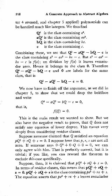
118 A Concrete Approach to Abstract Algebra
ter 4 stressed, and chapter 5 applied) polynomials can
be handled much like integers. We thus find
Q? is the class containing xz.
aQ2is the class containing ax2
.
bQ is the class containing bx.
c is the class containing c.
Combining these, we see that Q? — aQ2 — bQ — c is
the class containing xs — ax2 — bx — c. But x3 — ax2 —bx — c is /(x); on division by /(x) it leaves remain-
der zero. Hence it belongs to the class 0. Therefore
Q? — aQf — bQ — c and 0 are labels for the same
class, that is
Q3 - aQ2 - bQ - c = 0.
We now have to finish off the argument, as we did in
chapter 5, to show that we could drop the boldface
and write
Q 3 — aQ2 — bQ — c — 0,
that is,
AQ) = o.
This is the main result we wanted to show. But wealso have the negative result to prove, that Q does not
satisfy any equation of lower degree. This comes very
simply from considering residue classes.
Suppose someone claimed that Q satisfied an equation
pQ2 + rQ + s = 0. I suppose here that p, r, s are not all
zero. If someone says 0-Q2 + 0- Q + 0 = 0, we can
only agree with him. That is perfectly correct, but it is
trivial; if you like, you can reword the theorem to
exclude this case specifically.
Suppose, then, it is claimed that pQ2 + rQ + s = 0.
In terms of residue classes, this means that pQ2 + rQ +s = 0. pQ2 + rQ+ s is the class containing/w2 + rx + s.
The equation asserts that px2 + rx + s leaves remainder

Extending Fields 119
0 on division by x z — ax2 — bx — c. But this is so only
if p, r, s are all zero, and we have already excluded this
trivial case.
We have now proved all the assertions contained in
the theorem. Q.E.D.
It will be convenient to make a remark about the newfield while we still have in mind the symbols as defined
in the proof of the theorem. We want to show that the
facts given in the theorem completely replace the res-
idue-class approach so far as making calculations is
concerned.
With f(x) cubic, it is clear, on the residue-class ap-
proach, that we never need anything higher than a
quadratic in Q, to write down an element of the newfield. For the remainder, on dividing any polynomial by
a cubic /(*), will be at most a quadratic in x, and its
label will be at most quadratic in Q, How is this result
arrived at with the new approach?
The theorem does give us a way of getting rid of all
powers of Q above the second. For it states /(Q) = 0,
and this is equivalent to
Q 3 = aQ2 + bQ + c. (I)
(It was in anticipation of this equation that f(x) was
defined as x3 — ax2 — bx — c, rather than with positive
signs.)
Accordingly, we have a quadratic expression that can
always be substituted for Q 3. If we multiply both sides of
equation (I) by Q, we obtain
Q4 = aQ3 + bQ2 + cQ. (II)
Substitute in (II) the value of Q 3 given by (I). We find
Q4 = a(aQ2 + bQ + c) + bQ2 + cQ
= (a2T" b)Q2 T (ab -f
- c)Q -f- ac. (Ill)
It is evident that by continuing in this way, any

120 A Concrete Approach to Abstract Algebra
power whatever of Q can be expressed as a quadratic
in Q. Hence any polynomial in Q can be reduced to a
quadratic.
Thus, ifwe take two quantities of the form rQ 2 + sQ + t
and add or multiply them, the result is always expressible
in this form.
We can show, too, that every such quantity other
than zero has a reciprocal of the same type. Let g(Q) =rQ2 + sQ + t. By the H.C.F. procedure, applied to the
polynomials g(Q) and /(Q), we can find polynomials
u(Q) and v(Q) such that
g(QMQ) +/(QMQ) = 1.
But /(Q) = 0. Hence
g(QMQ) = l.
u(Q) is a polynomial in Q. Actually, the H.C.F. process
will yield a quadratic u(Q) and a linear v(Q). But wecan save ourselves the trouble of proving this by meansof the remark above, that any polynomial in Q can be
reduced to a quadratic.
Thus 1/g(Q) can be expressed as a quadratic in Q.
Division by g(Q) can be achieved by multiplying by
1/g(Q).
These considerations are intended to illustrate the
fact that the properties of the new field can be obtained
from the information contained in the theorem alone
—
that is, by purely algebraic calculations, without anymention of residue classes or the meaning of Q. Weappeal to residue classes to satisfy our scientific con-
science, to show that what we are doing is justified. But
once the foundations have been laid, we can proceed
purely by calculation—as, of course, mathematicians
did for centuries with V — 1 and V/
2 before the residue-
class explanation was thought of.

Extending Fields 121
The field formed by adjoining the element Q to the
field F is often denoted by F(Q). This, of course, has
nothing to do with the symbol for function, such as /(*).
For example, if R stands for the field of real numbers,
R(y/— 1) will stand for the field obtained from R by
introducing the new element y/— 1; that is, R(V- 1)
stands for the complex numbers.
Question: Verify by calculation that the elements
rV/
4 + s's/2 + t (r, s, t rational numbers) can be added,
subtracted, multiplied, and divided, the results always
being expressible in the same form. (This is the particular
case where /(x) = *3 — 2, so Q = V2, Q2 = V4.) Find,
in this form, the reciprocal of
's/a + 2^2 + 3.
Two Finite Fields
As an illustration of these ideas, we shall consider
two fields obtained as extensions of the arithmetic mod-
ulo 2. These fields contain only a finite number of ele-
ments so that they are very compact and easily surveyed.
The procedure, as explained earlier, is to select an
irreducible polynomial /(*), and then introduce a newsymbol, say Q, such that/(Q) = 0.
We first choose an irreducible quadratic for /(*);
later we study what happens when an irreducible cubic
is chosen. The irreducible quadratic has already been
touched on in various examples (pp. 106-107, questions
3, 4, 6, 10). The discussion of the irreducible cubic is
equally suitable for an example. After reading the ac-
count of the irreducible quadratic here, you may well
wish to work out the other question for yourself, and see
what properties you can observe or prove in the field
you obtain.
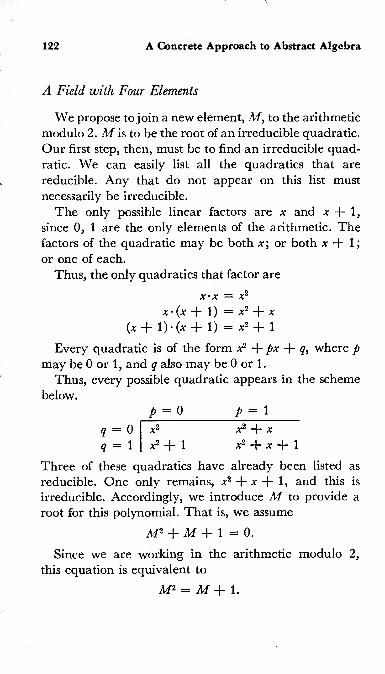
122 A Concrete Approach to Abstract Algebra
A Field with Four Elements
We propose tojoin a new element, M, to the arithmetic
modulo 2. M is to be the root of an irreducible quadratic.
Our first step, then, must be to find an irreducible quad-
ratic. We can easily list all the quadratics that are
reducible. Any that do not appear on this list must
necessarily be irreducible.
The only possible linear factors are x and x + 1,
since 0, 1 are the only elements of the arithmetic. Thefactors of the quadratic may be both x
;or both x + 1
;
or one of each.
Thus, the only quadratics that factor are
xx = x2
x - (* -f- 1) = x2 + x
(*+ l)-(*+ 1) = x2 +lEvery quadratic is of the form x2 + px + q, where p
may be 0 or 1, and q also may be 0 or 1.
Thus, every possible quadratic appears in the scheme
below.
p = 0 p = 1
q= o
q= 1
Three of these quadratics have already been listed as
reducible. One only remains, x2 + x + 1, and this is
irreducible. Accordingly, we introduce M to provide a
root for this polynomial. That is, we assume
M2 + M + 1 = 0.
Since we are working in the arithmetic modulo 2,
this equation is equivalent to
M2 = M + 1.

Extending Fields 123
(Justification. Add M2 to both sides of the earlier equa-
tion, and use 1+1=0 for the coefficient of M2 on
the left-hand side. M + 1 = M2is the result.)
By means of this equation, we can always replace
M2 by M + 1, and thus we never need to have the
square of M, or any higher power, left in an expression
:
we can always simplify until a polynomial is reduced to
linear form.
Thus, all our elements will be expressible in the form
aM + b, where a and b take the values 0, 1. So we have
the scheme:
6 = 0 b = 1
a = 1 M M + 1
a = 0 0 1
This shows that the new field contains only four ele-
ments 0, 1, M, M + 1.
The addition and multiplication tables for these four
elements are
:
0 1 M M + 1
0 0 1 M M + 1
1 1 0 M + 1 MM M M + 1 0 1
M + 1 M + 1 M 1 0
0 1 M M + 1
0 0 0 0 0
1 0 1 M M + 1
M 0 M M + 1 1
M + 1 0 M + 1 1 MThe addition table is easily obtained: we have only
to remember, since we are working modulo 2, that
1 + 1 and M + M are both zero.

124 A Concrete Approach to Abstract Algebra
In the multiplication table, we need to use the equa-
tion M2 = M + 1 . Thus
M-M = M2 = M + 1
M-(M+ 1) = M2 + M= (M + 1) + M = 1
(Af + 1) • (M + 1) = M2 + 2M + 1 = M2 + 1
= (M + 1) + 1 = M.
The values thus found have been entered in the multi-
plication table above.
On seeing this multiplication table for the first time,
students often comment on the pattern it displays—the
stripes running from northeast to southwest. It is inter-
esting to observe such a pattern. However, it is a mistake
merely to notice a pattern, and pass on.
Very often a mathematical discovery starts with an
observation of some pattern. Then one asks, “What is
this pattern? Why does it occur here? How can it be
made to yield a mathematical theorem or principle?”
After thought and analysis, one can often reach a result
much more definite and useful than the original recog-
nition of a superficial pattern. The next few paragraphs
follow the lines of an actual class discussion. All the
answers are those produced by the students.
First of all, then, what is the pattern we have seen?
If we leave out the border of zeros, the multiplication
table has the following pattern.
a b c
b c acabWhere have we seen this kind of pattern before? In the
arithmetic modulo n. In which table did it occur? In
the addition table: the addition tables always showed
this northeast-to-southwest striped effect. All the addition
tables had this general type of pattern : did any particular

Extending Fields 125
table actually reproduce the identical pattern above?
Yes: the arithmetic modulo 3. (See your answers to
questions on page 15-16.)
Our result is now rather more definite: the multiplica-
tion table in our field reproduces the pattern of the
addition table modulo 3. This is in itself quite striking.
We have the following correspondence.
Field
elements
1
MM + 1
Numbersmodulo 3
0
1
2
Multiplication in the first column corresponds to addi-
tion in the second column. What does that remind us of?
Logarithms. We could in fact use the table above exactly
like a table of logarithms, for example, to multiply Mby M + 1. Opposite M we find 1, opposite M + 1
we find 2. Add 1 to 2. The sum (modulo 3) is 0. Now wedecode (“take antilogarithms”). 0 stands opposite to 1.
So the answer is 1 ,which is correct.
What, then, is a logarithm? The usual definition is
that logb a — x if a = bx . A table of logarithms is just a
table of powers, read the other way round.
So our little table above suggests that there is some b
such that
1 = b\
M = b\
M+\ = b\
The middle entry here tells us what the base b of our
log table is: b = M. In fact, then,
1 = M\M = M\
M + 1 = M\

126 A Concrete Approach to Abstract Algebra
In our field, then, every element except zero is a power
of M.Why should modulo 3 come into it? Let us continue
to calculate the powers ofM :
M3 = M-M2 = M(M + 1) = M2 + M = 1,
M4 = M'M3 = M,M5 = M-M4 = M2
,
M6 = M-M5 = M3 = 1.
It is pretty clear now that, for any whole number n,
M3n = 1,
M3n+1 = M,M3n+2 = M2
.
Accordingly, if you want to find any power of M, say
Mk,where k is a whole number, all you need to know
is whether k leaves remainder 0, 1, or 2 on division by 3.
That is why modulo 3 comes into the picture.
A modular arithmetic always comes in when we are
dealing with roots of unity. For example (— 1)* is 1 if
k is even, — 1 if A; is odd.
It is clear that sooner or later the powers of an element
of the field must recur. Otherwise we could go on for-
ever, forming M, M2,Ms
,M4
,
- • •,and getting new ele-
ments all the time. But the field contains only four ele-
ments; the supply of new elements must give out pretty
quickly. This type of argument clearly applies to any
field with a finite number of elements.
Our inquiry naturally raises a number of general
questions. Gan an irreducible polynomial f(x) of any
desired degree k be found for the arithmetic modulo n
(n prime)?
If so, we can construct a field by adjoining an element
M for which f(M) = 0 is assumed. Will all the elements
of this field, apart from zero, be powers of M? Or is this

Extending Fields 127
property confined to the case we have just considered?
Or does it hold sometimes but not always?
The answers to these questions are known and can be
found in standard texts, such as Van der Waerden’s
Modern Algebra. You may derive some entertainment bycollecting evidence bearing on these questions and try-
ing to discover, or to prove, the answers for yourself.
Some relevant evidence is provided later in this chapter,
when we study a field with eight elements.
It may be worth noting a curious symmetry between
the elements M and M + 1
.
M is a root of the equation x2-f- x -}- 1 =0. So is
M + 1 .
If you add 1 to AT you get M + 1
If you add 1 to M + 1 you get M.If you square M you get M + 1
.
If you square M + 1 you get M.Every element of the field, except 0 is a power of M.Every element of the field, except 0, is a power of
Af+1.
This symmetry is significant and plays an important role
in more advanced theory.
A Field with Eight Elements
We now begin to construct another field. We shall
work much as we did on the field with four elements,
except that we shall begin by seeking an irreducible
cubic rather than an irreducible quadratic.
There are eight cubics, since in *3 + px1 + qx + r each
ofp , q, r can be 0 or 1 . As before, we begin by listing all
those that can be factored. A cubic can factor into a
linear factor and an irreducible quadratic, or it may

128 A Concrete Approach to Abstract Algebra
break up completely into linear factors. The following
list covers all the possibilities:
x(x2 + * + 1) = X3 + X2 + X,
(x + 1)(*2 + * + 1) = X3 + 1,
X’X’X = X3,
x-x(x + 1) = X3 + x2,
x • (* + 1 )2 = X3 + X,
(x + l) 3 = XZ + X2 + * + 1.
Two cubics remain. They are x3-f x + 1 and x3 + x2 + 1
.
These are the irreducible cubics over the arithmetic mod-
ulo 2. We could choose either of them. Suppose we
choose x3 + x + 1.
Our next step is to introduce Q with the assumption
Q3 + Q + 1 = 0, which is the same thing as saying
Q 3 = Q + 1 .
This equation shows that we need never keep Q 3 or
any higher power in any expression. All our elements can
be put in the form aQ2 + bQ + c. Earlier we arranged
Q*+l
O

Extending Fields 129
the four elements of the other field systematically in asquare (on p. 123). To arrange our present eight ele-
ments systematically, we need a cube.
The floor of the cube corresponds to a = 0, the ceiling
to a = 1 ;the front to b = 0, the back to b = 1 ; the
left to c = 0, the right to c = 1
.
In our earlier work, the powers of M gave us all the
non-zero elements of the field. Do the powers of Q dothe same now? To answer this, we calculate the powersof Q.
Q° = 1,
Q 1 = Q,
Q2 = Q\Q 3 = Q + 1, our basic assumption,
Q4 = Q • Q 3= Q* + Q 5
Q5 = Q.Q4 = Q3 + Q2 = Q2 +Q + 1j
Q6 = Q Q® = Q3 Q2 Q _ Q2 + 1}
Q7 = Q-Q6 ~ Q3 + Q = 1.
(The last step in finding Q5, Q 6
,and Q7 consisted in sub-
stituting Q -f 1 for Q 3,and simplifying, with the arith-
metic modulo 2.)
Q° through Q 6 are all different; they give us sevenelements of the field: zero is the eighth. Once again all
the non-zero elements are powers of a single element.
EXERCISES
1. What arithmetic modulo n plays the role for the field
with eight elements that the addition modulo 3 played for thefield with four elements?
2. Every non-zero element can be represented as a powerof Q. Is Q the only element with this property? If not, whatother elements have it?

130 A Concrete Approach to Abstract Algebra
3. The equation x3 + x + 1 = 0 has the root Q. Has it
any other roots in the field with eight elements?
4. The cubic x3 + x2 + 1 is irreducible over the arithmetic
modulo 2. Is it irreducible over the field with eight elements? Do
any elements of the field satisfy the equation xs + *2 + 1 =0?
5. If we had chosen x3 + x2 + 1 instead of x3 + x + 1 for
our irreducible f(x), would it have made any essential differ-
ence to the work? Should we have arrived at the same field?
6. Which powers of Q satisfy the equation x3 + x + 1 = 0.
Do you notice anything about these powers?
Terminology
Fields with a finite number of elements are known as
Galois Fields, in honor of the young French mathemati-
cian who first investigated them, rather more than a
century ago. The letters GF are used as an abbreviation
for Galois Field.
GF(2) is used to denote the arithmetic modulo 2, since
this contains two elements 0, 1. The field with the 4 ele-
ments 0, 1, Af, M + 1 is denoted by GF{2 2). The field
with 8 elements is denoted by GF(2 3).
Quite generally GF(pn) denotes a Galois Field with p
n
elements, where p is a prime number. (This is a slightly
confusing abbreviation. In it, pn has its usual algebraic
meaning, but GF must not be interpreted algebraically
as a product. GF is simply an everyday abbreviation like
UNESCO or NATO.)

Chapter i
Linear Dependence and Vector
Spaces
In chapter 6, we noticed in passing that the elements
of GF(2 3) could be arranged in the shape of a cube, while
those of GF(22) could be arranged in a square. GF(2)
of course has only the two elements 0, 1 and may be vis-
ualized with the help of a line.
0 1
Here is a hint that fields may have some kind of
geometrical aspect.
In this chapter we develop some ideas that will prove
very useful for the study of fields. The language of this
chapter is geometrical. “Linear” is connected with the
idea of “line”; “vector,” is derived from the Latin
verb “to carry,” and is associated with the idea of mov-
ing from one point to another. However, as was stressed
in chapter 1 we are concerned with structures, not with
meanings.
We shall not confine ourselves to geometrical applica-
tions, but we shall consider anything that has the same
structure as certain geometrical entities. It is, in fact,
very helpful to be able to pass quickly from one partic-
ular representation to another, now using a geometrical,

132 A Concrete Approach to Abstract Algebra
now a numerical, now a physical realization of a struc-
ture, so that we see the analogies between all of these
but are never tied to any one of them.
Let us start with a very physical example. You wish
to buy some nails and screws in a hardware store. The
storekeeper has observed that his customers usually buy
such things for fitting hinges (using six screws) or for
fixing cupboards to walls (using four screws and four
nails). He has all his screws and nails done up in little
packets, “The Home Handyman” with 6 screws, and
“The Complete Carpenter” with 4 screws and 4 nails.
If you want to buy screws and nails for some purpose
other than those envisaged by the storekeeper, and you
do not want to upset the store’s organization by asking
to have the packets opened, there are certain limitations
on what you can obtain. You can buy 26 screws and
8 nails by taking 3 Handyman packets and 2 Carpenter
packets, but you certainly cannot get 3 screws and
15 nails.
Any collection of screws and nails that you are able
to buy (without splitting packets) we shall call a possible
purchase or, more briefly, a purchase. We shall consider
purchases in their algebraic aspect, and we shall also
consider how to represent them geometrically.
What algebraic operations are possible with purchases?
The most obvious one is addition—the putting together
of two purchases. Thus 5 Handyman and 2 Carpenter
packets is a purchase; 3 Handyman and 7 Carpenter
packets is another purchase. The sum of these two pur-
chases is 8 Handyman and 9 Carpenter packets.
There is no obvious way of multiplying a purchase by
a purchase. A child would know what you meant by
adding a Handyman packet to a Carpenter packet, but
he would be puzzled to multiply them.
There is, however, one kind of multiplication that is

Linear Dependence and Vector Spaces 133
possible. We know what is meant by one purchase being
three times as large as another. If a purchase consists
of 2 Handymans and 5 Carpenters, three times this
purchase is 6 Handymans and 15 Carpenters.
Thus we can add a purchase to a purchase, but wecannot multiply a purchase by a purchase. We can how-
ever multiply a purchase by a number. This suggests a
final question: can we add a number to a purchase?
Imagine the following conversation.
Clerk. Is there anything else?
Customer. Yes. Three.
Clerk. Three more Carpenters, sir?
Customer. No. Just three.
Clerk. Do you want a metal three to put on your front
door?
Customer. No. Just the number three.
The clerk hopes it is a harmless lunatic he is dealing
with.
It is thus quite natural, in the situation described,
to say
Purchase -j- Purchase is defined.
Number X Purchase is defined.
Purchase X Purchase is not defined.
Number + Purchase is not defined.
How arbitrary this would look in abstract formula-
tion! “We have two sets of objects. The set P contains
elements pi, pi, pz, ••
•;the set M contains elements
^lj ^3j •
axiom 1. To any two elements pi, pi, of P there corresponds
an element of P, denoted by pi + pi.
axiom 2. To any elements pi of P and ni of M there cor-
responds an element nipi of P.
“We do not, however, define products of the type
pipi, nor sums of the type m + pi.” Why not, you won-

134 A Concrete Approach to Abstract Algebra
der. The reasonableness of the above passage appears
as soon as you recognize P as the set of all possible pur-
chase, and M as the set of natural numbers.
We now introduce a notation that is convenient for
our discussion of purchase, and that will have other
uses later.
Let (x,y) stand for “x screws andy nails.”
Let H stand for a Handyman packet and C for a
Carpenter packet. We can then write
H=(6,0) (1)
C = (4, 4) (2)
For the purchase that we considered earlier, consisting
of 3 Handymans and 2 Carpenters, we can write
3H + 2C = (26, 8) (3)
You can, of course, check this last equation by going
back to its meaning. However, since we are interested
in the formal aspects of this matter, we naturally try to
obtain rules for calculation with expressions of this kind.
We are guided, in making these rules, by what we knowabout the meaning of the symbols.
Suppose we are given
F - (a, b) (4)
G = (c, i) (5)
How shall we find F + G? We go back to the meanings
of F and G.
F stands for a screws and b nails.
G stands for c screws and d nails.
Putting these together,
F + G stands for {a + c) screws and (
b
+ d) nails.
So
F G — (a c, b d) (6 )

Linear Dependence and Vector Spaces 135
If we now look at equations (4), (5), (6), we can see
that these equations give a formal definition of F + G.
In the same way, if n is a number, we can show that
ri'F — (na ,nb) (7)
This is easily justified in terms of screws and nails. But
equations (4) and (7) themselves show by what rule nF
is obtained from F; we can use this rule without making
any reference to the meaning of F.
Graphical Interpretation
It is easy to illustrate what we have been considering
with ordinary graph paper. Some possible purchases are
shown in the following diagram, the number of screws
12,
10
8Nails
0
4
2
Screws
being measured horizontally and the number of nails
vertically.
You will notice that, starting from any point of this
set that you like, adding H always takes you 6 units to
the East. Adding C always takes you a certain distance
(actually 4V2 units) to the North-East,

136 A Concrete Approach to Abstract Algebra
This shows the relation of vectors to the word “I
carry,” and we could in fact explain vectors (as was
done in the early days of vector theory) as representing
displacements, (x, y) would then stand for “x inches to
the East and y inches to the North.”
Clearly, if operation F sends us a inches East and
b inches North, while G sends us c inches East and d inches
North, the combined effect of F and G (one operation
followed by the other) is to send us (
a
+ c) inches East
and (
b
+ d) inches North. Thus the addition procedure
defined by equations (4), (5), (6) above still holds good.
The operation F, repeated n times, will take us na inches
East and nb inches North; so this ties in well with
equation (7).
With these operations we are no longer restricted to
the natural numbers. We can have fractions and negative
numbers, with the usual understanding that — 2| inches
East means 2\ inches West.
Suppose PQR represents a piece of wire. We displace
this wire say an inch to the North-East. Every point of
ft'
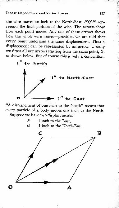
Linear Dependence and Vector Spaces 137
the wire moves an inch to the North-East. P'Q'R' rep-
resents the final position of the wire. The arrows showhow each point moves. Any one of these arrows showshow the whole wire moves—provided we are told that
every point undergoes the same displacement. Thus adisplacement can be represented by an arrow. Usually
we draw all our arrows starting from the same point, 0,as shown below. But of course this is only a convention.
, // , . ,
I To North
“A displacement of one inch to the North” means that
every particle of a body moves one inch to the North.
Suppose we have two displacements
:
F 1 inch to the East,
G 1 inch to the North-East.
C B

138 A Concrete Approach to Abstract Algebra
What is the combined effect of these? Consider Ffollowed by G. F would send 0 to A. G would send Ato B. The combined effect is to send 0 to B.
If we considered G followed by F, then G would send
0 to C. F would send C to B. The combined effect is
again to send 0 to B.
Thus the combined effect of the displacements repre-
sented by the arrows OA and OC is the displacement
represented by OB. It does not matter in which order
the displacements OA and OC are combined.
More generally, with
F a inches to the East, b inches to the North,
G c inches to the East, d. inches to the North,

Linear Dependence and Vector Spaces 139
the arrow OA represents the displacement F, the arrow
OC represents the displacement G, the arrow OB repre-
sents the combined effect.
We denote the combined effect by F + G. The par-
allelogram OABC (page 137, bottom) gives us a geomet-
rical way of visualizing vector addition. The algebraic
way we have already had : when F is (a ,b) and G is (c, d),
then F + G is (a + c, b + d). Note that this too appears
in the figure on page 138.
Vector addition, of course, plays an important part in
mechanics. It appears in the combination of forces,
velocities, and accelerations. Vectors pervade many
branches of theoretical physics—electromagnetic theory
for instance.
If A: is a number, kF is defined as the vector (ka ,kb).
This is the vector having the same direction as F, but
its arrow is k times as long. The diagram here shows Fand 2\F. F is OA. 2\F is OE.
Dimension of a Space
So far we have been talking of displacements so much
to the East and so much to the North. Such displace-
ments will get us anywhere we want on the ground.
If we want to rise in the air or bore into the ground,
we must consider displacements a inches to the East,
b inches to the North, c inches Up. Starting from a point
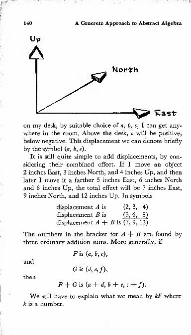
140 A Concrete Approach to Abstract Algebra
Up
East-
on my desk, by suitable choice of a, b, c, I can get any-
where in the room. Above the desk, c will be positive,
below negative. This displacement we can denote briefly
by the symbol (a, b, c).
It is still quite simple to add displacements, by con-
sidering their combined effect. If I move an object
2 inches East, 3 inches North, and 4 inches Up, and then
later I move it a farther 5 inches East, 6 inches North
and 8 inches Up, the total effect will be 7 inches East,
9 inches North, and 12 inches Up. In symbols
displacement A is (2, 3, 4)
displacement B is (5, 6, 8)
displacement A + B is (7, 9, 12)
The numbers in the bracket for A + B are found by
three ordinary addition sums. More generally, if
F is (a ,b, c),
and
G is (<7, £, /),
then
F T- G is (a + d, b -f- e, c + /)•
We still have to explain what we mean by kF where
A; is a number.
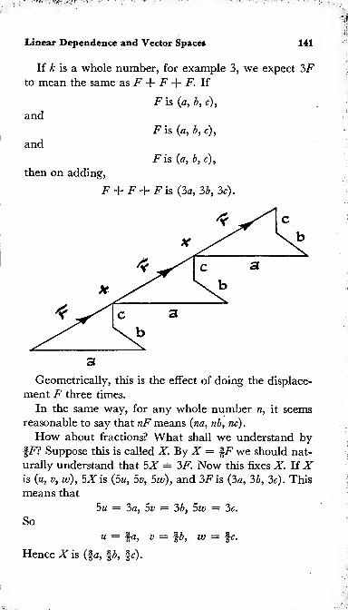
Linear Dependence and Vector Spaces 141
If A; is a whole number, for example 3, we expect 3Fto mean the same as F + F + F. If
and
and
F is (a ,b, c),
F is (a ,b, c),
F is (a, b, c),
then on adding,
F + F + F is (3a, 3b, 3c).
Geometrically, this is the effect of doing the displace-
ment F three times.
In the same way, for any whole number n, it seems
reasonable to say that nF means (na ,nb, nc).
How about fractions? What shall we understand by
fF? Suppose this is called X. By X = §F we should nat-
urally understand that 5X = 3F. Now this fixes X. IfXis {u, v, w), 5X is (5w, 5 i», 5w), and 3Fis (3a, 3b, 3c). This
means that
5m = 3a, Sv = 3b, 5w = 3c.
So
m = §a, v = %b, w = fc.
Hence X is (fa, %b, fc).

142 A Concrete Approach to Abstract Algebra
So the definition that
whenkF is (ka ,
kb, kc)
F is (a, b, c)
agrees with our ordinary ideas when £ is a natural num-
ber or a positive fraction. We shall still use this definition
when k is negative, like — 3, or irrational, like V:2.
Now let P stand for 1 inch to the East,
Q stand for 1 inch to the North,
R stand for 1 inch Up.
Earlier we had the symbol (2, 3, 4) for A. What is the
corresponding symbol for P? P is 1 inch East, nothing
North, nothing Up. So P is (1, 0, 0). In the same way, Qis (0, 1, 0), and R is (0, 0, 1).
Now A, being 2 inches East, 3 inches North, and
4 inches Up, could evidently be gotten by doing the dis-
placement P twice, then Q three times, and R four times.
This suggests that A = 2P + 3Q + 4R. We have reached
this conclusion by a geometrical argument. We can
check it algebraically.
Since P is (1,0,0), IP is (2, 0, 0)
Since Q is (0, 1,0), 3Q is (0, 3, 0)
Since R is (0, 0, 1), 4R is (0, 0, 4).
Adding, 2P + 3Q + 4R is (2, 3, 4), which is A.
Exactly the same argument shows that for F, the dis-
placement (a, b, c),
F = aP + bQ + cR.
By suitable choice of a, b, c, the vector F can be made
equal to any displacement.
Thus, when we are considering displacements of this
kind, any displacement can be gotten by adding suitable
multiples of three vectors, P, Q, R. If you think of P, Q, R

Linear Dependence and Vector Spaces 143
as ingredients, every F can be regarded as a mixture, in
suitable proportions, of these ingredients.
In our earlier work, when we did not allow displace-
ments Up, any displacement could be gotten by a suit-
able mixture of P and Q. Every journey can be achieved
by traveling East and then North (minus numbersaccounting for West and South).
Movement on the ground—or, more generally, in a
plane—is called movement in two dimensions. Move-ment East, North, and Up is called movement in three
dimensions. In the form “3D,” as applied to motion
pictures, this latter term has passed into the language of
the man in the street.
Q
ent mathematicians use the word “basis” with slightly
different meanings. In saying that P and Q form a basis
for vectors in this plane, we shall understand the fol-
lowing:
(i) Every vector F can be gotten by a suitable mixture
of P and Q.
(ii) Every vector F can be gotten in only one way as
a mixture of P and Q,
(iii) Every mixture of P and Q lies in the plane.

144 A Concrete Approach to Abstract Algebra
To illustrate these: P by itself does not form a basis,
since there are vectors in the plane that cannot be gotten
by moving Eastward—algebraically, that cannot be rep-
resented by kP. For example, the vector S with com-ponents (1,1) has the direction North-East. Geometri-
cally it is evident that S cannot be gotten by taking any
amount of P (that is, by traveling East for any distance)
.
Algebraically, kP is the vector {k, 0), and however wechoose k we cannot make this into (1, 1).
Condition (i) thus shows that P alone does not form a
basis. There are more things that can be done in a plane
than pure East-West travel.
Condition (ii) is intended to avoid extravagance. Wemight propose P, Q, and S (S was defined two paragraphs
earlier) as a basis. P + Q + S would then be the dis-
placement (1, 0) + (0, 1) + (1, 1) = (2, 2). But (2, 2)
could equally well be represented as 2S, or as 2P + 2Q,or as 3P + 3Q — S, or in many other ways. As S is itself
already a mixture ofP and Q, it is wasteful to bring S in.
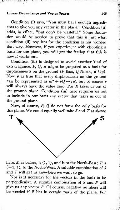
Linear Dependence and Vector Spaces 145
Condition (i) says, “You must have enough ingredi-
ents to give you any vector in the plane.” Condition (ii)
adds, in effect, “But don’t be wasteful.” Some discus-
sion would be needed to prove that this is just whatcondition (ii) requires for the condition is not wordedthat way. However, if you experiment with choosing abasis for the plane, you will get the feeling that this is
how it works out.
Condition (iii) is designed to avoid another kind of
extravagance. P, Q, R might be proposed as a basis for
displacements on the ground (
P
East, Q North, R Up).Now it is true that every displacement on the groundcan be represented as aP + bQ + cR, but of course c
will always have the value zero. For R takes us out of
the ground plane. Condition (iii) here requires us not
to include in our basis any vector that takes us out of
the ground plane.
Now, of course, P, Q do not form the only basis for
this plane. We could equally well take S and T as shown
here. S, as before, is (1, 1), and is to the North-East; T is
(— 1, 1), to the North-West. A suitable combination of S
and T will get us anywhere we want to go.
Nor is it necessary for the vectors in the basis to beperpendicular. A suitable combination of S and P will
give us any vector F. Of course, negative numbers will
be needed if F lies in certain parts of the plane. For

146 A Concrete Approach to Abstract Algebra
example, F might be taken as Q. How is Q to be gotten
by mixing S and P?
S is (1, 1),
P is (1, 0),
Q is (0, 1).
Evidently Q = S — P, which can also be seen geomet-
rically. The journey S, followed by — 1 to the East (1 to
the West) brings us 1 to the North, as required for Q.
-P
Linear Dependence and Vector Spaces 147
EXERCISES
1. Express S and T as mixtures of P and Q.
2. Express P and Q as mixtures ofS and T. Interpret geomet-
rically.
3. Show that the answer to question 2 could be obtained
from the answer to question 1, by solving the simultaneous
equations S = P + Q, T = —P + Q for P and Q.
4. Which of the following form a basis for vectors in a
plane? (i) The vectors (0, 1) and (1, 1). (ii) The vectors (1, 2)
and (2, 1). (iii) The vectors (1, 2) and (2, 4). (iv) The vectors
(1,5), (2,2), and (4,1).
5. Does any basis in the plane (i) consist of only one vector?
(ii) consist of three vectors?
6. If U is (a, b) and V is (c, d), the vector (p, q) will be ex-
pressible as xU + yV if x, y satisfy the equations
p = ax + cy
q = bx + dy.
Solve these equations for x and y.
If U and V form a basis, every vector (p, q) can be expressed
in the form xU + yV. That is to say, the equations above have
a solution, whatever p and q. Find the condition a, b, c, d must
satisfy if this is to be so.
(If your work seems to show that the equations can always
be solved, consider the case a = 1, b = 1, c = 2, d = 2. Thevectors (1,1) and (2, 2) do not form a basis. For these values
the equations cannot be solved when, for example, p — 1,
q = 0.)
You will have noticed that we had many ways of
choosing a basis for the ground plane, but that the basis
always contained two vectors—no more, no less.
In the same way, if we are allowed to move freely
(North, East, and Up), we can choose as a basis the three

148 A Concrete Approach to Abstract Algebra
vectors P, Q, R. Needless to say, there are many other
ways of choosing a basis, but however we do it, we al-
ways find that it consists of three vectors. That is what we
mean when we say that we live in three dimensions, while
a creature that can only crawl on the ground is confined
to two dimensions.
Now it seems fairly evident to us that a plane is some-
thing different from a space of three dimensions. How-
ever, someone might ask us, “How do you know that
the two things are distinct? Might there not be a space
such that, by one way of choosing your basis you found
it had three vectors, and by another way you found a
basis with two vectors in it?” We certainly do not expect
such a thing to be possible; but we are now challenged
to say why. Later a theorem will be given that meets
this question.
Coefficients
In the first part of this chapter, we considered packets
of screws and nails. Since we could only buy a whole
number of packets, we considered expressions such as
3H + 2C in which natural numbers came. Thus, at
this stage we considered aH + bC with a,
b natural
numbers. This led to the diagram on page 135, in which
the dots all lay in a certain region—between East and
North-East from the origin.
We could extend the network if we allowed a and b
to take positive or negative whole numbers as values.
Our dots would then extend in all directions, but of
course they would not fill the plane ;there would still be
spaces between them, as at present.
Now we have a choice in fixing our terminology. Shall
we say that a vector space must be like a plane—a con-
tinuous membrane, so to speak—or shall we accept a

Linear Dependence and Vector Spaces 149
network of points as forming a vector space, even if
there are intervals between the points?
For a book on algebra, there is no doubt about the
answer. We have talked about operations + ,•, —
,-r,
but nowhere have we said what we mean by “continu-
ous,” “near to,” or any such term. These are the ideas
of topology or analysis rather than algebra. Provided a
structure allows us to add, subtract, and multiply, weaccept it.
Accordingly, we shall have a good deal of freedom in
deciding what coefficients to allow. We might consider
expressions a
U
+ bV where U and V were given “things”
(of some kind) and a, b were required to be any one of
the following:
(i) Integers (positive or negative),
(ii) Rational numbers,
(iii) Real numbers,
(iv) Complex numbers,
(v) Numbers modulo 2,
(vi) Numbers modulo 3,
(vii) Polynomials in *, with real coefficients.
This by no means exhausts the possibilities. Some of
these structures we might be able to realize geometrically,
others we would be unable to draw. This does not
matter at all.
The following example calls attention to a possible
misunderstanding. Suppose we define U as being
inches to the East, V as being V3 inches to the North,
and require the coefficients a,b to be integers, positive
or negative. This gives us a perfectly good vector space,
of the “network” type. You will notice that irrational
numbers V2, V3 come into the definition of U and V,
while only integers are allowed for coefficients. It does
not matter that \^2 andV3 are not integers.

150 A Concrete Approach to Abstract Algebra
We are not doing anything worse here than when wetake screws and nails as our basic “things.” Here our
basic “things” are an arrow pointing Eastward, and an
arrow pointing Northward. One arrow happens to be
“s/2 inches long; the other happens to be inches
long. We then combine a times the first arrow with
b times the second arrow; a geometrical construction
shows the meaning of this statement. Thus it is quite
possible, in the definition of our basic “things” U, V,
to use numbers that would not be acceptable as coeffi-
cients a,
b.
In our hardware example, we used natural numbers
as coefficients. This was quite useful as an introduction,
to show how expressions like 2H + 3C came about.
However, the natural numbers suffer from the defect
that you cannot always subtract. You cannot take away
5 screws and 8 nails from 2 screws and 3 nails. In a vector
space (as this term is used by the majority of mathe-
maticians today), it is required that subtraction be al-
ways possible. That is, if L and M are two vectors, there
must always be a vector X such that L + X = M,and X is called M — L. That is why the natural num-bers are not on the list of suggestions for coefficients.
The set of “possible purchases,” mentioned at the begin-
ning of this chapter, thus does not constitute a vector
space. If we extended the definition to include negative
purchases—a customer returning several packets—then
it would constitute a vector space over the integers,
with H and C as a basis.
Specification of a Vector Space
We have now reached the stage where we can specify
what we mean by a vector space. A vector space involves

Linear Dependence and Vector Spaces 151
two sets of objects, rather intimately mixed. I shall call
these
(i) Things,
(ii) Numbers.
The numbers belong to a certain specified class. Bythe use of the word “number,” I do not imply anyconnection with, for instance, counting. By number I
just mean something that is going to be used, later on,
as a coefficient like a, b above. It must be possible to
add, subtract, and multiply numbers. To be more pre-
cise, I suppose the numbers to obey axioms (7) through
(P), (77), and (72). (In our main applications, the num-bers will be assumed to obey all the field axioms. Stu-
dents should be careful to note the point in the develop-
ment of the theory after which the results are true
ONLY for fields.)
The set from which the numbers are drawn will bedenoted by K.
There is no restriction on the kind of object that canplay the role of a Thing. In any particular example, weof course specify what is allowed as a Thing. Thingsmay be physical objects, ideas in the mind, marks onpaper, sounds of words, actions, operations. A Thingcan be, and usually will be, of a compound nature. Thuswe regard “3 screws and 2 nails” or “5 inches East and6 inches South” or “3x2 — 5xy + 6
y
2” as being a Thing.
The numbers of K may very well enter into the specifi-
cation of a Thing, as for example if we take
K : all real numbers.
Things: all displacements in the ground plane.
The real number 3^2, for example, enters into the
specification of “3^2 inches to the North-East.”
The Things form a vector space of n dimensions over
the numbers K if the following statements hold.

152 A Concrete Approach to Abstract Algebra
(I) Every Thing can be given a label (ai, a2 ,• •
•,an)
where <21,a2 ,
• • •,a„ are numbers from K. No Thing
has two different labels.
(II) To every possible label there corresponds one, and
only one, Thing.
(III) Corresponding to any two Things, A and B, there
is defined a third Thing, C, called the sum of Aand B. If A has the label (ax,
• ••
,an), B the label
(bi,• •
•,bn), C the label (ri,
• ••
,cn), then
ci = a\ + b\
c2 = 02 + b2
Cn — CLn~f" bn .
(IV) Corresponding to any Thing A and any number k,
there is defined a Thing D, called k times A. If
A has the label (ax,• •
•,
a„), D has the label
(Jc&iy* * *
,kdn) .
Some examples of vector spaces will help to make
these conditions clear.
Example 7.
K : the real numbers.
Things: the displacements in the ground plane.
We use (a, b) as a label for “a inches East and b inches
North.” This provides a label for every possible displace-
ment. There is a displacement corresponding to every
possible label. We never get two different labels for the
same displacement, nor two different displacements for
the same label.
We have already seen how statements (III) and (IV)
apply. We have here a space of 2 dimensions over the
real numbers.
Example 2.
K : the integers.
Things: all expressions ax + by + cz with whole
number coefficients a, b, c.

Linear Dependence and Vector Spaces 153
Addition of expressions and multiplication of expres-
sions by numbers are defined as in elementary algebra.
Thus, for example, the sum of 2x + 3y + 4z and
5x + 6y + 7z is lx + 9y + 1 lz; and 5 times 2x + 3y + 4z
is 10x + 1 5jy + 20z.
We choose the label (a, b, c) for the expression ax +by + cz. Thus (2, 3, 4) is the label for 2x -f- 3y + 4z. Noother expression gets this label. No expression has two
different labels.
Does statement (III) apply?
We take an example:
2x + 3y + 4z has label (2, 3, 4),
5x + 6y + lz has label (5, 6, 7).
If statement (III) holds, the sum should have label
(7, 9, 11).
In fact, it does so. One can show, by simple algebra,
that statement (III) applies generally.
Does statement (IV) hold? Again, we take an exam-
ple. The expression 2x + 3y + 4z has label (2, 3, 4). If
statement (IV) holds, 5 times the expression should have
label (10, 15, 20). It does; and we can show that this
always happens.
We have here a vector space of 3 dimensions over the
integers. Every expression ax + by + cz is a mixture of
x, y ,and z. x
, y, z form a basis. You may notice that x
has the label (1, 0, 0), y the label (0, 1, 0); z the label
(0 ,0
,1 ).
Example 3.
K : the real numbers.
Things : all quadratics ax2 + bx + c with real a, b,c.
This is a vector space of 3 dimensions over the real
numbers, x2,x, 1 form a basis, ax2 + be + c receives the

154 A Concrete Approach to Abstract Algebra
label (a, b,c). *2 has the label (1, 0, 0), x the label (0, 1,0),
1 the label (0, 0, 1).
Example 4.
K: the rational numbers.
Things: all numbers a + by/
2
with a, b rational.
We assign the label (a, b) to a + by/2. Thus 5 + 7a/2
would be labeled (5, 7). It is clear that only one Thing,
a + bV2, corresponds to the label (a ,b). But what about
the other way? Can two different labels give the same
Thing? Suppose they could;imagine that {a, b) and (c ,
d)
are two labels for the same Thing. This means that
a + bV
2
= c + dV2,_
a — c — (d — b)y/2.
If d — b is not zero, we can divide by it. Then
(a - c)/(d - b) = V2.
This gives V2 as a fraction, a rational number. But
this has been proved impossible. So d — b must be zero.
It follows that a — c is zero also. Hence d = b, a = c.
So the two labels are the same.
Statements (III) and (IV) can be checked without
difficulty. We thus have a vector space of 2 dimensions
over the rationals: 1 has the label (1, 0), y/
2
the label
(0, 1). Together 1 and V2 form a basis.
Example 5.
K: 0, 1 modulo 2
Things: 0, 1, M, M + 1.
The Things here form GF{22). All the Things are ob-
tained by letting a and b run through the values 0, 1 in
the expression a + bM. We have a vector space of 2 di-
mensions over K.

Linear Dependence and Vector Spaces 155
1 has the label (1, 0), and M the label (0, 1).
1 ,M form a basis.
Example 6.
K: the integers.
Things: a + %b, (a, b integers).
This has perhaps the appearance of a space of 2 dimen-
sions with (a, b ) as the label for a + \b. But then (3, 0),
(2, 2), (1, 4), (0, 6), and many others would all label the
same thing.
In fact, of course, whatever integers you choose for
a, b, the value of a + \b will lie in the set
These are all of the form \m where m is an integer.
We have a space of 1 dimension over the integers. Basis,
the single Thing, f . (m) is the label for \m.
Contrast example 4.
Example 7.
K: the integers.
Things: all numbers of the form ah
where a, b are integers.
Sum and product: as in arithmetic.
This, of course, is not a vector space over the integers.
If b is positive, abis an integer. If b is negative, say
b = —m, then ab = a~m = \/am and abis the reciprocal
of an integer.
Now 3_1 = 1/3 and 5"1 = 1/5, but 3”1 + 5"1 = 1/3 +
1/5 = 8/1 5, which is neither an integer nor the recip-
rocal of an integer. So A = 3_1
,B — 5
-1 are Things,
but A + B is not a Thing.
There is another way in which this structure fails to
be a vector space that is worth noting. Suppose we de-
cided to take {a, b) as a label for ab.

156 A Concrete Approach to Abstract Algebra
ah gets the label {a, b),
cd gets the label (c, d).
If statement (III) holds, ab + cd ought to get the label
(a + Cy b + d), but ab + cd
is not equal to {a + c){b+d\

Chapter 8
Algebraic Calculations
with Vectors
We saw in Example 2 (page 153) that linear expressions
of the form ax + by + cz constituted a vector space of
3 dimensions. Thus a vector space is no unfamiliar thing
;
if you have handled linear expressions in school algebra,
you already know a vector space and how it behaves.
But, more than this, vector spaces have very little indi-
viduality; they differ of course in dimension, but this is
not a very serious difference—if you can correctly per-
form algebraic calculations on expressions of the type
ax + by + cz, you will hardly find difficulties with the
type ax + by or the type ax + by + cz + dt. Vector
spaces also differ in the numbers K they employ: it
makes some difference whether a, b, c are integers, or
rational, or real, or numbers modulo 5—but again, not
very much difference; algebraic calculations with all of
these have much in common. Working with vector spaces
is accordingly much the same thing as working with linear
expressions in elementary algebra.
You may have noticed that all the equations we have
had connecting vectors have been linear equations, for
example
:

158 A Concrete Approach to Abstract Algebra
F = aP+bQ+cR (page 142)
Q — S — P (page 146)
Linear expressions are very simple to handle. Geomet-
rical questions, which otherwise might be difficult, can
sometimes be expressed in the language of vectors, and
thus converted into simple algebraic problems.
Example. Three wires radiate from a point 0. Thefirst wire is horizontal and points due East. The second
wire makes an angle of 45° with the horizontal and goes
North from 0. The third wire goes in a Northeasterly
direction, and rises 1 foot for every V2 feet in a hori-
zontal direction. Do the three wires lie in a plane or not?
Solution. We use the symbol {a, b,c) as on page 140.
The first wire evidently has the same direction as the
vector (1, 0, 0) = A, say. The second wire has the direc-
tion of the vector (0, 1, 1) = B,say. The third wire has
the direction of the vector (1,1,1) = C, say. (A diagram
or model will make these statements clear.)
Does C lie in the plane of A and B? To answer this
question we must translate into the language of vectors
“the plane of A and B.” This is not hard to do.
If we go any distance in the direction of A, and then
A

Algebraic Calculations with Vectors 159
any distance in the direction of B,the total displacement
is one lying in the plane of A and B.
The vector corresponding to “any distance in the
direction of A” is represented by sA, for some number s.
The vector corresponding to “any distance in the
direction of i?” is represented by tB, for some number t.
The combined effect of these displacements is gotten
by addition (see page 139). It is thus sA + tB.
Hence any vector in the plane ofA and B is of the form
sA ~f- tB.
Our question becomes, can we find numbers s and t
for which C = sA + tB?
This question can in fact be answered immediately.
We have
A = (1, 0, 0).
B = (0, 1, 1),
A + B = (1, 1, 1) = C.
So s = 1, / = 1 does the trick.
If we did not spot this, we should have to proceed as
follows:
A = (1, 0, 0). sA = (.r, 0, 0).
B = (0, 1, 1). /. tB = (0, t, t).
sA + tB = (.r, t, t).
We want, if possible, to make this equal to (1, 1, 1).
s = 1,t = 1 does this.
So the three wires do lie in one plane.
The connection of this work with linear expressions
appears most clearly if we use the three vectors P, Q, R
as defined on page 142. (The symbols A, B we are now us-
ing have of course no connection with the symbols A, Boccurring on pages 139-142.) Then
A = PB= Q + RC = P+ Q + R
160 A Concrete Approach to Abstract Algebra
and the question is, can we find numbers s, t so that
C = sA + tB? To see that s = 1, t = 1 provides a
solution requires no knowledge beyond very elementary
algebra.
Someone who was told to handle vector expressions
aP + bQ + cR “just like ax + by + cz in elementary
algebra” would probably find this quite a sufficient
guide for practical calculation. However, this prescrip-
tion is somewhat vague, and it will be as well to list the
properties we have in mind.
For definiteness, we shall take n = 4, so that our
vectors will have labels (01, a2 , <33, «4). But the arguments
apply equally well whatever natural number is chosen
for n.
The numbers, shown by small letters, ai, b2 ,k, and so
on, are supposed to obey axioms (7) through (9) and
(77). The vectors, or “Things,” are subject to statements
(I)-(IV) of page 152.
Denote by Pi the vector with the label (1, 0, 0, 0),
Denote by P2 the vector with the label (0, 1, 0, 0),
Denote by P3 the vector with the label (0, 0, 1, 0),
Denote by P4 the vector with the label (0, 0, 0, 1).
It requires no ingenuity to verify the results listed
below. Several of these are left as exercises.
(V.l) Corresponding to any two vectors, A and B,
there is a vector C, called A + B. This is given
in statement (III), page 152.
(V.2) A + B = B + A. This follows from the latter
part of statement (III), and from axiom (3) for
numbers aT,br .
(V.3) A + (P + C) = (A + B) + C.
(V.4) There is a vector 0 such that A + 0 = A for
any vector A.

Algebraic Calculations with Vectors 161
(V.5) The equation A + X — B has a unique solution
X, whatever the vectors A and B. X is called
B - A.
(V.6) For any number k and any vector A, the product
k'A is uniquely defined. This is the earlier part
of statement (IV).
(V.7) For any number k and any vectors A, B,
k-(A + B) = (k-A) + (k-B).
(V.8) For any numbers a, b and for any vector A,
(a + b)-A = (a- A) + (/b-A ).
(V.9) For any numbers a, b and for any vector A,
(<ab) •A = a -(b-A)
(V.10) Every vector A is expressible in the form
a\P\ + &2P2 + Q3P3 + aiPi.
(This is for n — 4. In general, aiPx + • •• + anPn of
course replaces the expression here.)
EXERCISES
1. Prove statements (V.3, V.4, V.5, V.7, V.8, V.9, V.10)
above, the statements (I)-(IV) of page 152, and the axioms
( 1)-(9) and (77) for the numbers being given as known.
2. Prove from the statements (V.l)-(V.IO), that for the vec-
tor 0 and for any number k,we have k-0 = 0.
3. Prove that, if 1 is the unit of the number system, for anyvector A, we have 1-A = A. (Begin with V.10. Use V.7 andV.9.)
4. Prove that, 0 denoting the zero of the number system, andA being any vector, we have 0-A = O.
5. Prove that, if —A is used as an abbreviation for 0 — A,
then — A =(— 1)-^4.

162 A Concrete Approach to Abstract Algebra
6. What statements from (V.l)-(V.IO) are used in obtain-
ing the following results? (i) 2 • (34 + 4B) + 5 • (34 + 45) =
7- (3A + 45). (ii) 3•(5^4 + 65) = 154 + 185.
The above examples show how closely calculations
with vectors resemble elementary algebra; in fact, as
was mentioned earlier, linear expressions ax + by +cz + dt actually constitute a vector space.
Thus, in order to work with vectors, no new formula,
no new procedure needs to be memorized.
Statements (I) through (IV) of page 1 52 are needed
if one is in doubt whether or not some particular struc-
ture is a vector space.
Statements (V.l) through (V.10) resemble several of
the axioms for a field (page 27). Of course, they contain
nothing resembling field axiom (70), that provides for
division. These statements, (V.l) through (V.10), can
always be appealed to, if our right to perform some for-
mal algebraic manipulation with vectors is challenged,
or if we are in doubt whether or not a particular step
is justified. In some treatments of vector spaces, state-
ments (V.l) through (V.10) form the starting point,
rather than statements (I) through (IV).
Linear Independence
Suppose, in elementary algebra, we consider all ex-
pressions of the form au + bv ~h cw, where a, b, c are
integers and
« = x+ y + z + ?,
v = x + 2y + 3z + At,
w = x + 4y + 7z + 10£.
At first sight, you might think these expressions con-
stituted a vector space of 3 dimensions, basis u, v, w, with
(a, b, c) as the label for the expression au + bv + cw.

Algebraic Calculations with Vectors 163
However, consider the two cases
(i) a = 1 b = 5 c = 3,
(ii) a = 3 b = 2 c — 4.
We find
u + 5v + 3w = 9x + 23y + 37z -f- 5l£,
3m + 2m + 4za = 9* -f 23jy + 37z + 51 1 .
That is to say, the labels (1, 5, 3) and (3, 2, 4) both
describe the same Thing. This, however, is contrary to
statement (I). Since
u + 5v + 3w = 3u T" 2v + 4w,
it follows that
2u — 3v + w = 0. (1)
In fact, w = — 2u + 3v, so any expression au + bv + cw
could be written au + bv + c(— 2u + 3v). This equals
{a — 2c) u + (b + 3c)v, which is a mixture of u and v
alone. For example, u + Sv + 3w and 3m + 2v + 4wabove are both expressible as — 5m + 14m.
Thus it now appears that we have a vector space of
only 2 dimensions, with u, v as a basis. But perhaps this
is not yet the end of the story; perhaps m, v can be re-
placed by something even simpler. We now examine
this possibility.
Suppose we use (a, b) as the label for the expression
au + bv. Can one expression receive two labels? Suppose
it could;suppose (p , q) and (r, s) represented the same ex-
pression, that is,
pu + qv = ru + sv. (2)
Then
We write
(p — r)u + (q — s)v = 0.
f = p - r

164 A Concrete Approach to Abstract Algebra
Nowu = x-\-y-\-z-\-t,
v = x + 2y + 3z + At.
For fu + gv to be zero, we must have (as is seen by con-
sidering the coefficients of x, y, z, t
)
f + g — 0
/+ 2£ = 0
/+ 3^ = 0
f+4g = 0
(5)
The only solution of these simultaneous equations is
/ = 0, g = 0. By equations (3), this means that p — r,
q = s. And this means that (p, q) and (r, s) are one and
the same label.
So it is impossible for one expression to receive two
distinct labels. With u, v as a basis, all the requirements
of statements (I)-(IV) are met, and our expressions
thus form a vector space of 2 dimensions.
In this investigation, one or two ideas have occurred
that are of value for the theory generally, so that it is
worth while to introduce names for them.
In testing whether u, v formed a basis for a space of
2 dimensions, we considered the mixture fu + gv. Wefound that this was zero only when both / and g were
zero. The only way of mixing u and v so as to obtain
zero was to take none of either.
We then say that u, v are linearly independent.
Generally, we say that n vectors uh w2j• •
•,un are lin-
early independent if the only way to make the mixture
ciui + C2U2 + • • • + cnun zero is to make c\ — 0, r2 = 0,
* '') Cn ~ 0.
On the other hand, we had above u, v, w for which the
mixture 2u — 3v + w was zero. This is a genuine mix-
ture; it is not just “none of u,none of v, none of
Accordingly, we say that u, v, w are linearly dependent.

Algebraic Calculations with Vectors 165
definition. If n vectors
,
«i, M2, • ••
, Mft satisfy a linear
equation,
C\U\ + C2U2 + * * • + CnUn = 0,
other than the trivial equation,
Omi -j- OM2 “t~* •
• 4~ 0un = 0,
which is satisfied by any set of n vectors, we call the vectors
“linearly dependent.”
You will notice that “linearly independent” is another
way of saying “not linearly dependent.” A set of vectors,
Mi, • ••
,Mn,
must be one or the other.
Geometrical Interpretation
Geometrical examples of vector fields are helpful for
illustrating the meaning of linear independence.
For instance, on page 142 we met vectors P,Q,R whichrepresented an inch to the East, an inch to the North,
and an inch Up, respectively. Are these linearly inde-
pendent or not? That is, can we find a genuine mixture
of them that is zero? If we take cfP + c2Q + c3R, this
represents the displacement c\ inches to the East, c2
inches to the North, c3 inches Upwards. It is clear that
this gives the zero displacement only if ci — c2 = cs = 0.
That is, only the trivial mixture gives zero. HenceP, Q, R are linearly independent.
If, on the other hand, we take the vectors P, Q, S of
page 144, we have P + Q — S = 0. The vectors are
linearly dependent.
Quite generally, if U, V, W are three vectors in
geometrical space of 3 dimensions, they are linearly
dependent if they satisfy a non-trivial equation.
aU+bV +cW = 0.
Then the journey aU (which is in the same direction as

166 A Concrete Approach to Abstract Algebra
U), followed by the journey bV and the journey cW,
brings us back to the point where we started. Evidently
this means that U, V, W lie in a plane.
EXERCISES
By a model or diagram make clear to yourself how the vectors
listed below are situated in space. Hence determine whether
or not each set is linearly independent. Check your conclusions
algebraically.
1 . A = (1,1,0), B = (-1, 1,0), C =(0, 0, 1).
2. A = (2, 3, 0), B = (10, 1, 0), C =(1, 1, 0).
3. A = (0, 1, -1), B = (-1,0, 1), c = (1 ,
- 1,0).
4. A = (0, 1, 1), B = (1, 0, 1), c =( 1 ,
1,0).

Chapter 9
Vectors Over a Field
The processes we are soon to use involve division
by a number. From now on, we assume that our number system
forms a field.
On page 159 we saw that the vectors of a plane wereall of the form sA + tB.
In the same way, all the vectors that lie in a line are
of the form sA. Those that fill a 3-dimensional space
are of the form sA + tB + pC.
It is thus natural to study mixtures of a given set of
vectors. We may in this way obtain vector spaces that
do not correspond to our geometrical ideas derived from
the physical world. By considering mixtures of linear
expressions in ten variables we could construct, alge-
braically, vector spaces of any number up to 10 dimen-
sions. Needless to say, we cannot visualize such spaces
geometrically, though we may be helped in dealing with
them by analogies drawn from our physical experience
of three dimensions. Vectors in such spaces are not with-
out practical interest. In intelligence testing, for instance,
a candidate might be subjected to ten examinations. If
candidate A scored (ai, ai, • ••
, flio) in these examina-
tions, his performance would specify a vector in 10
dimensions. If candidate B scored bi, • ••
, biQ and candi-

168 A Concrete Approach to Abstract Algebra
date C scored a, ••
•, do, one might find, perhaps, that in
each test C’s score was the sum of 4’s and B’ s. This we
could write as C = A B. Or C’s marks might be,
in each examination, the average of T’s and B’s. Or
again, ifA scored full marks on test 1 ,and almost nothing
on the others while B scored high marks on test 10 and
nothing on the others, we could say that A’s and B s
abilities lay in different directions. All of this goes quite
naturally in the language of vectors, and in fact vectors
are used considerably in the theories of intelligence. Weare, then, concerned with mixtures of vectors, whether
these can be illustrated in physical terms or not.
We saw on page 163 that a mixture of three vectors
might sometimes produce a vector space of only 2 dimen-
sions. It is desirable to have a systematic way of deter-
mining the dimensions of the space generated by a col-
lection of vectors. (The space formed by all possible
mixtures of a given set of vectors is said to be generated
by these vectors.) This is quite simple to do. The process
depends on the two following principles.
principle i. The space generated by a set of vectors is
unaltered if any vector P is replaced by kP, where k is any
non-zero number.
principle ii. The space generated by a set of vectors is
unaltered if any two vectors P, Q of the set are replaced by
P, Q — sP where s is any number whatever.
Principle I, applied to a set of three vectors A, B, C,
states that kA, B, C generate the same space, that is,
any mixture of kA,B, C is a mixture of A, B, C, and con-
versely. That a mixture of kA, B, C is a mixture of
A, B, C is almost obvious. That a mixture of A, B, C
can always be expressed as a mixture of kA, B, C appears
from the equation
aA + bB + cC = (a/k) • (kA) + bB + cC.
Vectors Over a Field 169
No new idea is needed to prove this principle for anynumber of vectors.
The way in which principle II is proved is also clear
from the particular case of three vectors. We want to
show that P, Q, R and P, Q - sP, R generate the samespace. We write
U = P,
V = Q — sP,
W= R.
It is to be shown that any mixture of U, V, IT is a mix-ture of P, Q, R, and conversely. That a mixture of U,V, IT is a mixture of P, Q, R is obvious. But since
P = U,
Q= V+sU,R = W,
it is also obvious that any mixture of P, Q, R is expressible
as a mixture of U, V, W.The proof for any number of vectors follows exactly
the same lines.
Principle II can be applied repeatedly. For instance,
by applying it three times, one can see that (P, Q, R, S)and (P, Q — aP, R — bP, S — cP) generate the samespace.
Great caution is needed to avoid jumping to unwar-ranted conclusions. One might think that P, Q, R andP — Q, Q — R, R — P would generate the same space.This, however, cannot be derived by any number ofapplications of principle II, and is in fact untrue; con-sider for example the case when P, Q, R are all equal.
Conditions for a Space of n Dimensions
Suppose now we take any n vectors Pu P2,• •
•,Pn, and
consider all the vectors of the form afPi + a2P2 + • •• +

170 A Concrete Approach to Abstract Algebra
anPn • Do these form a space of n dimensions? Conditions
(II), (III), (IV) of page 152 are automatically satisfied,
(fli, <22,‘
•, an) being regarded as the label for aiPi +
G2P2 + • •• + anPn . The only doubt is in regard to the
latter sentence in condition (I). As we saw in the ex-
ample on page 163,this can fail: two different labels may
correspond to the same thing.
What is the condition for this failure? If (ai, • ••
,an)
and (bh ••
•,bn) are two labels for the same vector, this
means that
a\Pi + aiPi + • •• + anPn — b\P\ + 62P2 + • •
• + bnPn,
whence
(«1 — 61) -Px + ((22 — 62) 'P2 + • *• + (an — bn) • Pn = 0 .
Now (ai,• •
•,an) is not the same as {b\, • •
•, bn)- This
means that at least one of the coefficients above is not
zero. Hence, Pi, P2 ,
• ••
,Pn are linearly dependent, for
they satisfy a non-trivial equation (see definition, page
165 ).
Accordingly, if Pi, • ••
,P„ are linearly independent,
the failure of condition (I) cannot occur. All the condi-
tions (I)-(IV) are then satisfied, and we have the fol-
lowing theorem.
theorem. If Pi, •••, Pn are n linearly independent vec-
tors, they generate a space of n dimensions; that is, the totality
of vectors of the form a\Pi anPn constitute a space of
n dimensions.
A Standard Form
We now consider two examples in which it is immedi-
ately evident that a set of vectors are linearly inde-
pendent. These examples are significant. It will be
shown later that any set of vectors can be reduced to
this form by means of principles I and II.
Vectors Over a Field 171
Example. What is the dimension of the space gen-
erated by P, Q, R, S here specified?
P = x + 4y — I7z + 3 1— 2u,
Q = v + 5z — 81* + 39m,
R — z -f- At “f" 111 m,
S = t- 13M.
By the theorem above, we shall be sure that the space
is of 4 dimensions, if we can prove P, Q, R, S linearly
independent.
Suppose P, Q, R, S satisfy an equation
aP + bQ + cR + dS = 0.
Consider the coefficient of *. x appears only once on the
left-hand side in the term ax. Hence, a — 0. Accordingly,
bQ + cR + dS = 0.
Now y appears only in the term by. Hence, b = 0. Wesubstitute b = 0 in the equation, and go on to consider
the coefficient of z. This shows c = 0. Finally, from the
coefficient of t, we see d = 0.
Hence, P, Q, R, S satisfy only the trivial equation
with all coefficients zero. Hence, by definition, they are
linearly independent. So the space generated by P, Q,
R, S is of 4 dimensions.
You will notice in this example that the coefficients
(4, -17, 3, -2 inP; 5, -81, 39 in Q; 4, 111 in R; -13in S) are never mentioned in the proof. The proof de-
pends only on the fact that the non-zero coefficients form
the following pattern.
j* * * *
j* * *
j* *
1 *
It is also possible to have examples in which the pattern

172 A Concrete Approach to Abstract Algebra
shows steps rather than a diagonal edge, for example
the following.
-j*******
^* * * *
1 * *
1
Question: Show that a space of 4 dimensions is gener-
ated by the vectors P, Q, R, S where
P = x-\-y-{-z + t Jr u + v + w + s,
Q = t "-f- 2u 2v 2w -f- 2s,
R — v + 3w + 3s,
S = s.
In example 2 on page 153, we saw that the label
(a, b, c) can be attached to the expression ax + by + cz.
Our two examples above could equally well be expressed
by means of such labels.
Thus, the first example would show that a space of
4 dimensions is generated by the vectors
(1, 4, -17, 3, -2),
(0, 1, 5, -81, 39),
(0, 0, 1, 4, 111),
(0, 0, 0, 1, -13).
It is good to be able to follow the argument in either
form of notation. It is, of course, essentially the same
argument in either notation. One can pass from a ques-
tion stated in bracket notation—that is, with signs such
as (a, b, • ••
,k)—to the linear expression notation, by the
process used on page 159.
In the two examples we have just had, we may say
that the system P, Q, R, S is in standard form. In the first
example, P contains the symbol x, which is not in any
later expression Q, R, S. Q contains y, which is not in
R, S. R contains z, which is not in S. S contains t. (S is

Vectors Over a Field 173
not followed by any expression. So all we require of Shere is that it should not be identically zero. If it were
identically zero, we should simply omit it, since it wouldmake no contribution to the space.)
In the second example, P contains x, which is not in
any later expression Q, R, S. Q contains t, not in R, S.
R contains v, not in S. And S contains s.
These remarks should convey what is meant by “stand-
ard form.”
EXERCISES
1. Define formally when n linear expressions X\, • ••
,Xn in
m symbols x\, • • •
,xm are in standard form.
2. Make clear to yourself how you would recognize that n
vectors expressed in bracket notation were in standard form.
(The verbal definition of such a property is often difficult andtedious. The idea of standard form can certainly be grasped
by students who are unable to formulate it verbally. For our
purposes, the ability to recognize standard form is importantj
the verbalization, less so.)
Reduction to Standard Form
Our principles I and II allow us to make chains of,
arguments such as the following
:
Space generated by A, B, C= space generated by A, B — 2A, C by (II)
= space generated by A, B — 2A, C — 3
A
by (II).
We thus move from the set of vectors A, B, C to the set
A, B — 2A,C to the set A, B — 2A, C — 3A. These sets
of vectors are of course distinct. We could not write
that these sets were equal. But they have the property
that they generate the same space.

174 A Concrete Approach to Abstract Algebra
Accordingly, when we speak of reducing a set of vec-
tors to standard form, this is a brief way of saying that
we are looking for another set, a simpler set, that generate
the same space as the original set. For example, if
A = x + 5y + 12 z,
B = 2x + Uy + 33z,
C = 3x -f 9y + z,
the argument above leads us to
A = x + 5y + 12z
D = B - 2A = y+9zE = C - 3A = -6y - 35 z.
A, D, E generate the same space as A, B, C. NowA, D, E are not yet a standard set. But they are nearer
to standard form than A, B, C since x occurs in A but not
in B, C.
To complete the reduction to standard form, we
apply principle II again, and replace (A, D, E) by
(A, D, E + 6D). This yields
A = x + 5y + 12z,
D = y + 9z,
F = E + 6D = 19z.
Finally, by principle I, the expressions A, D, F can be
replaced by A, D, F/ 19, and standard form is thus
attained.
A = x + 5y + 12z,
D = y + 9z,
G = 2 .
A, B, C generate the same space as A, D, G \evidently
this is a space of 3 dimensions.
Question: There is an even simpler set of three vectors
that generates this space. What is it?
The procedure followed in reduction to standard form

Vectors Over a Field 175
should be clear. First we select a symbol (x) that actually
occurs in A. By “actually occurs 5’ I mean that its coeffi-
cient is not zero. Suppose, then, that A contains the
term ax. By principle I, we can replace A by (1/a) -A.
We thus have an expression
P = (\/a)‘A = x + •••.
If B contains bx, we replace B by B — bP, which does
not contain x. In the same way, we can replace C, con-
taining cx, by C — cP, which contains no x.
Thus we arrive at a set P, Q, R, S, • ••
,in which P
alone contains x. We set P on one side. We can nowforget about x, since Q, R, S, • •
•,do not contain it. We
choose a symbol y that actually occurs in Q, and follow
the same kind of procedure to replace R, S, • •
,by ex-
pressions free from y. We continue until a standard form
is reached.
Example. Reduce A, B, C to standard form, where
A = x y z 2t + m,
B = 2x + 5y + Sz + It + 5m,
C — x + 2y + 4z + 2t — u.
A contains x. We subtract from B and C multiples of Aso chosen that x disappears. We thus reach
^4 = x + y T" z -j- 2t -j- u,
D — B — 2A = 2>y + 6z + 3t + 3m,
E = C — A = + — 2m.
The coefficient of y in D is 3. So we use principle I
and consider ^Z). (It does not matter if such a step intro-
duces fractions. We are working with thefield of rationals.
Actually, no fractions occur in this example.)
A = x -}- y H- z T 2l -f* m,
F = \D = y + 2z + t + m,
E = y + 3z — 2m.
176 A Concrete Approach to Abstract Algebra
Finally, we have
A = x + y -f- z It -\~ u,
F = y + 2z + t + w,
G = E — F = z — t — 3u,
which is in standard form.
Example. Reduce to standard form the expressions
u, v, w of page 162. These expressions, you may remem-
ber, generated a space of only 2 dimensions. We shall
see how this appears in the work.
u = x+y-\-z+ t,
v — x + 2y + 3z + At,
w = x + Ay + Iz + 10?.
x occurs in the top row. We use principle II to get
rid of it in the other rows.
u — x + y + z + t,
p = v — u = y + 2z + 3/,
q = w — u = 3y + 6z + 9t.
y occurs in p. We get rid ofy in the third row by form-
ing q — 'ip. This, however, is Oy + Oz + 0;, the vector
zero. It makes no contribution to the space generated,
and is accordingly omitted. Thus the standard form is
u — x + y + z + t,
p — 4" 2z -f- 3t.
The two vectors u, p generate the same space as the
original three vectors u,
v, w.
The fact that q — 3p is zero shows that u, v, w are
linearly dependent. For q = w — u, and p — v — u.
Substituting for p and q we obtain
0 = q — 3p = (w — u) — 3(v — u),
= 2u — 3v + w,
as in equation (1) of page 163.

Vectors Over a Field 177
EXERCISES
Reduce the following systems to standard form. Whenever a
zero vector appears in the work, verify that the corresponding
vector in the original system is a mixture of the vectors which
precede it. (In our last example, the third vector in the process
of reduction is zero; this corresponds to the fact that the third
vector, w, of the original system u, v, w can be expressed as
— 2a + 3v.) Find the relationship in each system.
1. A = x+ y + z,
B = x + 3y + 3z + 2t,
C = 2x + 3y + 6z + At + 3t/.
2. A = x + 2y + 3z + At,
B = 5x + 6y + 7z + 8*,
C = 9x + lOy + llz + 12#,
D = 13x + 14y + 15z + 16*.
3. A = x — 2y + z,
5 = * + jy— 2z,
C = — 2x 4“ yd- z.
4. ^4 = x — y,
B = y - z,
C = —x + z.
5. ^4 = x + y,
R = y + z,
C = x +z.
We have had several examples in which the appear-
ance of a zero vector in the reduction process indicated
that a vector of the original system was a mixture of the
preceding vectors. We have not, however, proved that
this must be so.
The proof requires only one point to be established.
In our worked example on page 176, we had q — 3p = 0.

178 A Concrete Approach to Abstract Algebra
p and q were linear expressions in the original symbols
u, v,w. It seems evident that substitution for p and q in
terms of u, v, w must give a relation au + bv + cw = 0.
There is, however, one loophole that must be filled; it
might be that a,b, c all happen to be zero. In that event
we have not shown u,v, w to be linearly dependent.
In actual fact q — 3p = 2u — 3v w and the co-
efficient of w is 1. This is no accident. The process we
have described is such that the coefficient of the last vector
involved is bound to be 7. This by itself is sufficient to show
that we are not dealing with the trivial equation where
all coefficients are zero.
We still have to establish the statement just made,
that the coefficient is 1.
For definiteness, let us suppose that in the reduction
of A, B, C, D, • ••
,a zero vector appears at the third step.
We review the process of reduction. Let a, b, c, d, -,
stand for numbers that appear in the work. These have
no connection with any symbols previously used.
We suppose A contains x, perhaps not with coeffi-
cient 1, but with non-zero coefficient. We can make
the coefficient of * become 1 by multiplying with a
suitable constant a. Thus aA — x + • • • .
We now subtract suitable multiples of this expression
from B, C, • ••
,to get expressions free from x. These ex-
pressions will be of the form B b(aA), C c(aA), .
Now we suppose B — b(aA) contains y with non-zero
coefficient. The coefficient can be made equal to 1 by
multiplying by a suitable constant d. Thus
dB — dbaA = y + • • • •
We now subtract e times the expression above from
C — caA
;
we choose e so that y does not appear in the
result. We get the expression C — caA — e{dB — dbaA).
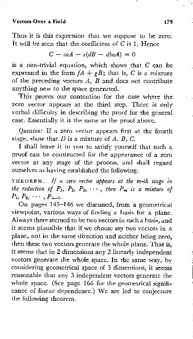
Vectors Over a Field 179
Thus it is this expression that we suppose to be zero.
It will be seen that the coefficient of C is 1. Hence
C — caA — e(dB — dbaA) = 0
is a non-trivial equation, which shows that C can be
expressed in the form fA + gB;that is, C is a mixture
of the preceding vectors A, B and does not contribute
anything new to the space generated.
This proves our contention for the case where the
zero vector appears at the third step. There is only
verbal difficulty in describing the proof for the general
case. Essentially it is the same as the proof above.
Question: If a zero vector appears first at the fourth
stage, show that D is a mixture of A, B, C.
I shall leave it to you to satisfy yourself that such a
proof can be constructed for the appearance of a zero
vector at any stage of the process, and shall regard
ourselves as having established the following.
theorem. If a zero vector appears at the m-th stage in
the reduction of Pi, P2 ,P3, • •
•,
then Pm is a mixture of
Plj P2, ' "•
5 Pm-1-
On pages 145-146 we discussed, from a geometrical
viewpoint, various ways of finding a basis for a plane.
Always there seemed to be two vectors in such a basis, andit seems plausible that if we choose any two vectors in a
plane, not in the same direction and neither being zero,
then these two vectors generate the whole plane. That is,
it seems that in 2 dimensions any 2 linearly independent
vectors generate the whole space. In the same way, byconsidering geometrical space of 3 dimensions, it seems
reasonable that any 3 independent vectors generate the
whole space. (See page 166 for the geometrical signifi-
cance of linear dependence.) We are led to conjecture
the following theorem.
180 A Concrete Approach to Abstract Algebra
theorem. In space of n dimensions,any n linearly inde-
pendent vectors generate the whole space.
It may help to see how this is proved if we consider
a particular example. Linear expressions of the form
ax + by + cz + dt constitute a space of 4 dimensions.
Suppose we have 4 expressions of this type, which are
known to be linearly independent. Then by mixing
these 4 expressions, it should be possible to obtain any
expression of the form ax + by + cz + dt.
Our 4 expressions can be reduced to standard form.
The expressions are linearly independent; no one of
them can be a mixture of the preceding ones; hence, by
the theorem of page 179, it is impossible for a zero vector
to appear in the reduction. (For if a zero vector did
appear, it would prove that one of the original vectors
was a mixture of the others.) Accordingly, the reduction
must go to its full length. There must be 4 vectors in the
standard form.
But there is only one way of getting 4 vectors in the
standard form, namely by means of the following pat-
tern.
A = x + ey + fz + gt,
B = y + hz + kt,
C = z + mt,
D = t.
We cannot possibly have a pattern like those on page 172,
in which long steps appear, and several letters x, y, z, • ••
,
drop out between one line and the next. For if we did
have this, we would have used up all our letters x, y, z, t
before we reached the fourth expression, D. Only by the
utmost economy, dropping one letter only at each line,
can we reach four lines. (We are compelled to drop one
letter at each stage. The definition of standard form
requires it. See the explanation on page 173.)

Vectors Over a Field 181
Thus the standard form A, B, C, D must be of the
type shown above. (There is, of course, nothing to pre-
vent some or all of the numbers e, /, g, h, k, m being zero.)
But now we can clearly obtain any expression ax +by -T cz + dt by a suitable mixture of A, B, C, D. Bytaking aA, we obtain the correct coefficient for x. Byadding a suitable multiple of B to aA, we can make the
coefficient of y correct, without altering the coefficient
of x. This would in fact give us aA + {b — ae)B, but the
details of the calculation are not helpful. By adding a
suitable multiple of C, we make the coefficient of z cor-
rect, without disturbing the coefficients of x and y.
Finally, by adding a suitable multiple of D, we obtain
the correct coefficient for t.
This mode of approach generalizes immediately to n
linear expressions in n variables xi, X2, • ••
,x„. The stages
in the argument are the following.
(i) The n expressions being independent, the standard
form must contain n expressions.
(ii) A standard form with n expressions in it musthave the form
A\ = xi +A 2 = x2 +A3 — X3 + • • • •
(iii) Any linear expression a\X\ + a2x2 -f • • • -j- anxn
can be gotten by taking suitable values a, c2, • ••
,cn in
c\A\ + C2A2 + • •• + c„A„.
Anyone who has understood the procedure for n = 4
will see that no new idea is needed to prove the general
case.
One final objection has to be met. We have taken a
particular example of a vector space, namely, linear ex-

182 A Concrete Approach to Abstract Algebra
pressions. But the theorem may be needed for some other
example of a vector space—say, for a geometrical space.
However, the first few pages of chapter 8 pointed out
that work with vectors was essentially the same as work
with linear expressions.
There are two ways of presenting the proof outlined
above in a form that shows it to be quite general.
1. In a vector space of n dimensions, every vector
is expressible as a\Pi + ciiPi + • •• + anPn . (See (V.10)
on page 161, and the explanation of Pi, Pi, • ••
,on page
160.) But this is a linear expression in Pi, Pi, • ••
,Pn . We
simply rewrite our earlier proof. Whenever xi occurs wewrite Pi instead. For x2 we write Pi, and so on.
2. Alternatively, we may use the label (ai, ai, • ••
,an)
for a vector in space of n dimensions, as on page 152. Thestandard form, for 4 dimensions say, will then appear as
A = (1, e, f, g),
B = (0, 1, h, k),
C = (0. 0, 1, m),
D = (0, 0. 0, 1).
The argument that any vector (a, b, c. d) can be ex-
pressed as a mixture of A, B, C, D follows essentially the
same lines. aA has the first number inside the bracket
correct. By bringing in B, we can make the second num-ber correct also. And so on. The whole proof can be
carried through in this notation.
The somewhat informal discussion we have just had
contains all the ideas needed for the proof of the theorem.
If you understand these ideas, you can verify that the
theorem is established. You can, if you like, write out a
formal proof. I do not give a formal proof in full, since
it would not be needed by anyone who has understood
these ideas, and would be meaningless to anyone whohas not.

Vectors Over a Field 183
We now have our final theorem of this chapter.
theorem. Any (n + 7) vectors in a vector space of n di-
mensions are linearly dependent.
Proof. Let the vectors be V\, V2 ,• •
•,F„
,Vn+i- It may
be that Fi, V2 ,• •
•,Vn are linearly dependent, being con-
nected by a relation ciVi + C2V2 + • •• + cnVn — 0,
where ci, • ••
,cn are not all zero. If so, we have
ClVl + C2V2 + • •• + CnVn + 0- Vn+1 = 0.
Since ci, • ••
,cn are not all zero, the coefficients in this
last equation are not all zero; that is, Fi, • ••
,Vn+\ are
linearly dependent.
So the theorem holds if Fi, • ••
,Fn are linearly de-
pendent.
Suppose then that Fi, • ••
,Vn are linearly independent.
Then, by the preceding theorem, any vector in the
space can be expressed as mixture of Fi, • ••
,F„. Hence
F„+i can be expressed as a mixture of Fi, • ••
,F„. Hence
Fi, • ••
,Vn+i are linearly dependent.
Thus the theorem holds in either case, and is proved.
On page 170 we proved that n linearly independent
vectors generated a space of n dimensions. Why then, it
might be asked, did we find it necessary to prove on
pages 180-182 that, in a space of n dimensions, any n
linearly independent vectors generated the whole space?
Is it not obvious that they generate the whole space?
For instance, someone might say, “take the case n — 2.
We have a plane; we take any two independent vectors;
they generate a plane—isn’t it obvious that this plane
must be the plane we started with?” It is indeed plausible
that it should be so. However, the chain of reasoning
just given assumes a certain result, namely that one
plane cannot be contained in another plane—this to be
understood in the sense that you cannot remove certain
points from a plane, and still have a complete plane re-

184 A Concrete Approach to Abstract Algebra
maining. More generally, if S and T are spaces of n
dimensions, and T is contained in S, then T is identical
with S. If one w-dimensional space lies in a second
n-dimensional space, then it completely fills it.
Now this result sounds very reasonable, but we have
to prove it. And, in effect, that is what we did on pages
180-182.
On page 148 the question was raised whether a space
might be at one and the same time a space of n dimen-
sions and a space of (n + 1) dimensions. It seemed un-
likely, but again unlikely things do happen—for instance,
there is a curve that completely fills a square; it is as
well to have a proof. The last theorem of this chapter
supplies the proof. In space of (n + 1) dimensions there
are n + 1 independent vectors—for example the vectors
Vi = (1, 0, 0, • •• , 0),
Vz = (0, 1, 0, •• , 0),
Fa = (0, 0, 1,•
•, 0),
n+l = (0> 0>
In space of n dimensions there cannot exist (n -f- 1) inde-
pendent vectors. Hence it is impossible for a space of
n dimensions to be a space of (n + 1) dimensions.

Chapter io
Fields Regarded as Vector Spaces
We have now proved some results for vector spaces,
but it is far from evident that these results will tell us
anything interesting about fields. In fact, some very use-
ful theorems about fields can be obtained.
To see how this happens, we review the procedure of
modern mathematics. The underlying idea of modernmathematics is to extract the essence of any proof, andseparate it from purely accidental aspects. In this waygenerality is obtained.
If you want to write a paper in modern algebra, youlook at a theorem somebody else has proved, and yousee just what he has used to prove it. For example, the
theorem that any quadratic has at most two roots wasoriginally proved for numbers. We examine the proof
and ask, “What properties of numbers does it use?” Wefind that it uses only the properties of numbers expressed
by axioms (7) through (72). This means that the proof
can be written in such a way that it applies to any set of
elements—not necessarily numbers—that obey axioms
(7) through (72).
So, without having used any real originality, we canstate a more general theorem: “In any structure, the

186 A Concrete Approach to Abstract Algebra
elements of which obey axioms (7) through (72), a quad-
ratic has at most two roots.”
We can now shorten this statement by bringing in a
technical term, “field.” Any structure, we say, for which
axioms (7) through (72) hold, will be referred to as a
field. Our theorem then takes the form, “In any field a
quadratic has at most two roots.”
A most important point should be noticed here; the
misunderstanding of it frequently causes confusion. Thequalification for being a field is positive, not negative.
That is to say, to be a field, a structure must satisfy
axioms (7) through (72). It is not disqualified from being a
field because it obeys other axioms in addition to (7) through (72).
There is an obvious reason for taking it this way. Theproof that a quadratic equation has at most two roots
uses axioms (7) through (72) only: so it applies to any
structure for which these axioms hold. The proof no-
where requires that the structure does not satisfy other
axioms. Real numbers, for instance, do satisfy other
axioms. There is the relation a < b, “
a
less than b,”
which is defined, and for which a system of axioms holds;
for example, it is an axiom that if a < b and b < c, then
a < c. Not all fields permit such a relation to be defined;
you would, for instance, find difficulty in defining an
order relation for the arithmetic modulo 5; again, we do
not use the symbol < for complex numbers. However,
the symbol < does not occur anywhere in the proof that
a quadratic has at most two roots. For the proof of this
theorem, it is entirely irrelevant whether the structure
has a relation a < b or not.
Thus, it is correct to say, “The axioms for a field do
not require a < b to be defined.” It would be incorrect
to say, “No structure in which a < b is defined is a field.”
In the same way the definition of “human” does not
require the possession of unusual physical strength,

Fields Regarded as Vector Spaces 187
American citizenship, or the wearing of a hat. But a
strong, American, hat-wearing individual is still to be
regarded as human; and all theorems that can be de-
duced from the axioms specifying humanity will be true
for such an individual. We do not think of “a humanbeing,” “a strong creature,” “an American,” “a hat
wearer” as being distinct objects. Rather these terms
emphasize different aspects of objects—or, it may well
be, different aspects of one single individual.
Thus, there is no contradiction between our having
proved, in exercise 7 on page 31, that the numbers
a + by/2 (with a, b rational) form a field, and on page 1 54
that they form a vector space of 2 dimensions over the
rationals. The usual objection is, “You can multiply
a + by/2 and c + dV 2, but you cannot multiply twovectors.”
The mistake here is again that of using the tests nega-
tively rather than positively. The basic property of a
vector space of 2 dimensions is that every element of it is
a mixture of two basic ingredients only. Now every num-
ber a -f- by/
2
is a mixture of 1 and y/l. By using this
property (in the form of the more precise statements we
had earlier), we can prove for the numbers a + by/
2
all
the theorems appropriate to spaces of 2 dimensions.
The fact that y/2 can be multiplied by V2 corresponds
to the aspect of this structure as a field. We cannot deal
with this aspect by means of the vector axioms.
The useful fact is that a + by/
2
is simultaneously a
vector space and a field. We can prove for it both the
theorems appropriate to vector spaces and to fields. In
this way we may be led to new results, obtained by com-bining these theorems.
In terms of our earlier illustration, we suppose it a
theorem that human beings are conscious of what is

188 A Concrete Approach to Abstract Algebra
happening, and that a hat-wearer’s head is warm. Wecan deduce that a human being wearing a hat is con-scious of warmth in the head. This result unites the twotheories: it cannot be proved in either theory alone. Ahuman being may have a cold head in the absence of a
hat. A lower animal, although wearing a hat and hencehaving a warm head, may not be conscious of the
warmth.
There is a property of the numbers a + bV2 that will
serve to illustrate this theme, and lead us to a more gen-
eral result.
Every number of the form a -f- bV
2
satisfies an equa-tion, with rational coefficients, which is quadratic (or
simpler in particular cases). For if
x = a + bV2,
x — a = 2,
(x — a) 2 = 2b 2.
Hence x2 — 2ax + a 2 — 2
b
2 = 0.
This is an equation with rational coefficients.
This method works all right in this particular case, butit does not generalize easily. For instance, it is true that
every number a + b^/
2
+ c's/A satisfies a cubic equa-
tion over the rationals, and that every number a + bV
2
+ cV3 + 6 satisfies an equation of the fourth degreeover the rationals; a, b
,c, d of course represent rational
numbers. One can easily construct more and more com-plicated examples of such theorems. The simple method
used above for a + iV2 does not enable us to see the
truth of these more complicated theorems. We accord-ingly look for a method that will generalize.
We return, then, to proving that a -\- bV
2
satisfies a
quadratic and look for a more illuminating proof.
A quadratic expression px 2-fi qx + r may be written

Fields Regarded as Vector Spaces 189
P' x2 + <l’ x + that is to say, it is a mixture of x 2
,x
,
and 1. We want to show that, for some rational numbers
p, q, r, this mixture will be zero. Let us take a particular
case, say x = 3 + 5V2. What are x 2,x, and 1?
1 =1,
x = 3 + 5\/2,
x2 = 59 + 30V2.
We seek to make a mixture of these three things zero.
Now, from the equations above,
px 2 + qx + r = (59P + 3q + r) + (30p + 5q)Vl.
As 59p + 3q + r and 30p + 5q are rational if />, q, r arerational, we can only make the above mixture of 1 andV2 zero by making
59p + "bq + r = 0 (1)
30p + 5? =0 (2)
Here we have two equations in the three unknowns/>, q,
r. Our theorem will be proved if we can show (i)
that non-trivial solutions exist, (ii) that some such solu-
tion makes p, q, r rational. The trivial solution p = q—
r = 0 of course is useless.
In this particular case, we can solve the equations,and verify that the solution is rational. However, we areseeking to extract some general principle.
The language of vector spaces helps us to do this.
px2 + qx + r • 1 =0 with rational p, q, r is another wayof saying that *2
, *, 1 are linearly dependent over K,the rationals.
Now, if 1, V2 are chosen as a basis, x2 has the label
(59, 30); x has the label (3, 5); 1 the label (1,0).
Equations (1) and (2) can be combined in the vectorequation
PC59, 30) + q(3, 5) + r(l, 0) = (0, 0).

190 A Concrete Approach to Abstract Algebra
But we know that any 3 vectors in 2 dimensions are
linearly dependent. So we can be sure that numbers
p, q, r, not all zero, exist which satisfy the above equation.
We need these p , q, r to be rational. Gan we be sure of
fulfilling this condition? We are working in the frame-
work of Example 4 on page 154. K is the field of rational
numbers. The numbers a, b that appear in any label
(a, b) are rational. The linear dependence of vectors
A, B, C means that pA + qB + rC = 0 with p, q ,r ele-
ments of K, not all zero. All the work proceeds within the
field K. It may help you to see this, if we work through
the proof that (n + 1) vectors in n dimensions are linearly
dependent, applying its procedure to the particular case
we have here, namely that the three vectors
A = (1, 0),
B = (3, 5),
C = (59, 30),
in 2 dimensions are linearly dependent. We should first
express A and B in standard form; this gives us two vec-
tors which form a basis for the whole space. Hence C is
expressible as a mixture of these. In fact,
B - 3A =(0, 5).
D = iB - iA =(0 ,
1 ).
A and D make the standard form. Evidently
C = 59A + 30D,= 59A + 30(iB - fA),
= 41A + 6B.
The numbers 1, 0, 3, 5, 59, 30 that occur in the labels
for A, B, C are necessarily rational. In the calculation,
we start with these numbers and perform addition, sub-
traction, multiplication, and division, but no other operation
is used. Accordingly, we stay always within K, the field
of rationals. We are bound to arrive at a rational solu-
tion p, q, r.
Fields Regarded as Vector Spaces 191
In this particular case, C — 6B — 41
A
= 0 : so p — 1,
q = — 6, r — —41, and x = 3 + 5\/2 satisfies x2 —6x — 41 =0. This, of course, is the same equation that
we should have obtained by applying our first method.
For this particular case, the second method is longer. Its
value lies in the fact that it applies to other cases. Thepurpose of the method, too, is not so much to calculate
the equation, as to show that an equation exists.
The work above shows that the theorem “Any (n + 1)
vectors in n dimensions are linearly dependent” can be
stated in elementary algebra. For suppose the vectors are
Vi with label (ah bh a, • ••
, gi),
V2 with label (a2,b2, c2, • •
•, g2),
Fn-j-i with label (an+i, rn-j-i, 3 ^71+1)3
where all the numbers a\, • ••
, gn+i belong to a field K.
The linear dependence of these (w + 1) vectors meansthat there are numbers pi, p2,
• ••
, pn+1, belonging to Kand not all zero such that p\V\ + p2V2 + pn+\
V
n+i= 0.
That is,
O-lpl + a2p2 -T * * * + On+lpn+i = 0,
b\p\ + b2p2 + • •• + bn+ipn+i = 0,
g\p\ + g2p2 + ’ '* + gn+lpn+1 = 0
,
so we have the theorem. If n equations in (n + 1) unknowns,
of the type shown above, have all their coefficients lying in a field
K, then these equations have a solution pi, p2,• •
•, pn+i com-
posed of elements of the field K, not all zero.
It is essential to include the words “of the type shownabove.” For instance, the three equations in four
unknowns
x+jy+ z + r = 1,
x + 2y + 3z + 4r = 2,
3x + ly + 12* + 17r = 3,

192 A Concrete Approach to Abstract Algebra
have no solution, as is easily verified if you regard r as
known, and try to solve for x, y, z. But these equations
are not of the type specified, since they have non-zero
constant terms 1, 2, 3.
This example also shows that the theorem is not trivial.
Having fewer equations than unknowns does not always
guarantee the existence of a solution.
We now use the method developed above to show that
x = a + b\/
2
+ 4, (a, b, c rational), satisfies an equa-
tion px% + qx2 + rx + s = 0, where p, q, r, s are not
all zero.
We noted on page 121 that the numbers t + u\/
2
+v\^4, with t, u, v rational, form a field. Since x belongs
to this field, x2 and x3 also belong to the field, by field
axiom (2). We could work out x 2 and x 3 in terms of a,b, c,
but this work would be wasted. All that matters for the
latter part of the proof is that x2 and x 3 are of the form
t + mV72 + flV
74. Accordingly, we write
1 = !,
x = a + b^/
2
+ r'V/4,
x2 = d + eV2 + fy/4,
x3 = g + h\/2 + ky/4,
where d,
e, /, g, h, k could be expressed in terms of a, b, c,
but all we really need to know is that these symbols
represent rational numbers.
We could now consider pxz + qx 2 + rx + s and show
that it would be zero if the four quantities p, q, r, s sat-
isfied the three equations
pg + qd + ra + s = 0,
ph qe + rb = 0,
pk + qf + rc — 0 .

Fields Regarded as Vector Spaces 193
We know that three such equations in four unknownsalways have a rational solution. Hence we know that
there are rational numbers p, q, r, s, not all zero, for
which px3 + qx2 + rx + s = 0, and our theorem is
proved.
In order to explain this proof, I have had to bring in
symbols d, e, f, g, h, k. But really I have not made any
calculations with these symbols. If I wanted to prove that
a + b's/2 + c\/A + d\/8 + eX^16 (a, b, c, d, e rational)
always satisfies an equation of the fifth degree over the
rationals, I should pretty well use up the whole alphabet
in explaining the proof. But the proof would not contain
any new idea. It is therefore natural to coin a name for
such a situation, to have a brief way of indicating that
this proof works. That name we already have: “vector
space.”
Our proof that every number a + b's/2 -f- cs/A satis-
fies a cubic equation can now be stated very briefly.
The rational numbers being denoted by K, the totality
of numbers t + us/2 + vX^A, with t, u,v rational, con-
stitutes the field K(\//2).
We now argue let x = a + b's/2 + c's/4. x is an ele-
ment of K(y/'2) . Since 2) is a field, x2 and *3 are also
elements of K{y/2). 1 is an element of K^T).Hence 1, x, x2
,x3 are elements of iC(V
/2).
But every element of K(s/2) is a mixture of 1, '\/2,
</4, with rational coefficients. Hence K{'s/2) is a vector
space of 3 dimensions* over K. Hence any four elements
of it are linearly dependent over K. Hence, for rational
* 1, 2
,
vT form a basis since they are linearly independentover K. But we do not even need to prove this. If they were
linearly dependent, K{ ^2) would be a space of less than 3 dimen-sions, and the proof would be even stronger than it is now.

194 A Concrete Approach to Abstract Algebra
numbers p, q ,r, s, not all zero, we have pxz + qx2 +
rx + s = 0. Q.E.D.
Question 1: If w stands for the real number such that
w7 = 2 and s = a + bw + cw2 + dw 3 + ew4 + fwh +where a, b
,c, d
,e> /, g are rational numbers, prove that
s satisfies an equation of the seventh degree with rational
coefficients. (This question is intended to show the econ-
omy of thought and statement made possible by using
the vector terminology, as compared with the notation
of elementary algebra.)
Question 2: Do the elements a + bx/2 + cV 3 + dx/
6
form a vector space over the rational numbers K? (a, b,
c, d rational numbers) . Of what dimension? What is the
degree of the equation with rational coefficients satisfied
by the general element of this correction?
Question 3: Let m — V2 + V^. Calculate m 2 and m 3.
Do 1, m, m 2,m 3 form a basis for the space considered in
question 2? What is the simplest equation over the ra-
tional that is satisfied by m? What are the other roots of
this equation? (The equation for m can be found quite
easily by elementary algebra.)
Question 4: An irrational number r satisfies an equa-
tion f(x) = 0, which is of degree n and irreducible over
the rational numbers K. Find a basis for K(r), regarded
as a vector space over K. Of how many dimensions is it?
What is the degree of the equation with rational coeffi-
cients satisfied by an arbitrary element of K(r)?
In our examples, we have taken K as the field of ra-
tional. Often indeed, we are interested in knowing
whether an element satisfies an equation with rational
coefficients. But we might also be interested to knowwhether it satisfied an equation with roots drawn from
some other field, F.

Fields Regarded as Vector Spaces 195
We have the following general theorem. SupposeF is any
field,and G is a field that contains F. Suppose G is a vector space
of n dimensions over F; that is to say, there are fixed ele-
ments bi, b2 ,• •
•,bn of G such that every element of G
can be represented in the form afb\ + a2b2 + • •• + anbn
by choosing suitable elements ah a2 ,• •
•,an of F. Then
every element of G satisfies an equation of degree n {or less)
over F.
For instance, if R denotes the field of the rationals, Fmight be Z?(V:2) and G might be F(V3). That is, westart with the rationals, R. F is obtained by bringing in
the new element V2; anything that can be gotten byadding, subtracting, multiplying, and dividing with ra-
tional numbers and Vz belongs to F. In fact, every ele-
ment of F can be expressed in the form p + q's/2, with
rational p , q. We use the letters u, v to denote elements
of F.
G is obtained from F by allowing the free use of the
extra symbol v^3. In fact, every element of G can be put
in the form u -f- &V3, where u, v belong to F.
Thus, in this example, b\ = 1 and b2 = V3 are the
fixed elements of G. a\ = u and a 2 = v are variables,
representing elements of F. Thus G is a vector space of 2
dimensions over F, and every element of G satisfies anequation of the second degree—that is, a quadratic
—
with coefficients in F.
For example, x = 'V/2 + V/
3isan element of G, with
a\ — V2 and a2 = 1.
Evidently (x — V2) 2 = 3, which simplifies to
*2 _ 2V2 x - 1 = 0.
This is a quadratic equation over F. The coefficients
are 1, — 2V2, — 1, all of which lie in F. It is not a
196 A Concrete Approach to Abstract Algebra
quadratic over the rationals R, since — 2V2 is not in R.
If we wish to obtain the equation over R satisfied by
Vl + V3, we write the quadratic above in the form
x2 - 1 = 2V2 x.
Squaring gives
(x2 - l) 2 = 8x 2,
whence
x4 - 10x 2 + 1=0.
This equation is of the fourth degree, which is quite
consistent with our theorem. For in u + vV 3, the general
element of G, the quantities u and v are elements of F;
that is to say, we may write
u = c + dy/2,
v — h + ky/2,
where c, d, h, k are rational.
Thus, the general element of G is
(c + dV2) + (h + kV2) V3or
c + dV2 + hV3 + kV6.
G is thus a vector space of 4 dimensions over R, with
1, V2, V3, y/
6
as a basis. Accordingly, any element of
G must satisfy an equation of the fourth degree at most,
with rational coefficients. Thus,
G is a vector space of 2 dimensions over F.
G is a vector space of 4 dimensions over R.
Any element of G satisfies a quadratic equation if
coefficients from F are allowed, but an equation of the
fourth degree is all we can guarantee if only rational
coefficients are allowed.

Fields Regarded as Vector Spaces 197
Finding the Equation of Lowest Degree
for Any Element
We have already met the principle that x satisfying anequation of degree n over any field K is the same as
1, x, x2,
• ••
,xn being linearly dependent over K. (See
pages 189-194.)
Thus, if x satisfies an equation of degree n, but noequation of degree less than n, then 1, x, x 2
,• •
•,x" will
be linearly dependent, but 1, x, x 2,
• ••
,xn_1 will be
linearly independent.
Thus, it is possible to find the value of n by forming the
quantities 1, x, x2,x 3
,
• ••
,and seeing at what point linear
dependence first happens. The standard form for vectors
gives a systematic way of doing this. The appearance of
a zero vector is the signal for linear dependence havingarisen.
Example. Find the degree of the simplest equation
over the rationals satisfied byx=v/2 + 'V
/3.
It saves rearrangements if we take our basis in the
order 1, Js/2, V6, V3 so that (a, b, c, d) is the label for
a + bV2 + CV6 + dV:3.
1 has label (1, 0, 0, 0),
x = V2 + v/3 has label (0, 1, 0, 1),
x 2 = 5 + 2V"6 has label (5, 0, 2, 0),
x3 = 11 V2 + 9V3 has label (0, 11, 0, 9),
x4 = 49 + 20V6 has label (49, 0, 20, 0).
There is no point in calculating further. We now havefive vectors in 4 dimensions. These must be linearly
dependent; but, conceivably, linear dependence mighthave arisen even before x4 was reached.
The vectors of the standard form are

198 A Concrete Approach to Abstract Algebra
1 with label (1, 0, 0, 0),
x with label (0, 1, 0, 1),
|(x 2 — 5) with label (0, 0, 1, 0),
— ^(x3 — llx) with label (0, 0, 0, 1).
No zero vector has appeared, so 1, x, x2,x3 are inde-
pendent and generate the whole space, x4is 49 times the
first vector added to 20 times the third vector of the
standard form above. That is,
x4 = 49-1 + 20-K*2 “ 5),
whence x4 — 10x2 + 1 =0 as we expected from our
earlier work. We have now demonstrated, by using a
vector procedure, that x does not satisfy any simpler
equation over the rationals.
This type of example is included here not so much be-
cause we wish to perform calculations of this kind, but
so that you can become used to thinking of elements of
fields as vectors. This idea is important for the general
theory.
Question: Find the degree of the simplest equation
over the rationals satisfied by V/
3 — V"2. Also find the
equation.
Must a Field Have a Dimension
Over a Sub-field?
Often one field G contains another field F. (Then Fis called a sub-field of G. Thus the rationals are a sub-
field of the reals because the reals contain the rationals.)
We have had examples in which G was a vector space of
n dimensions over F. Must this always happen? If a field
G contains a sub-field F, must G be a vector space of n
dimensions over F?
We must first get one difficulty out of the way. Sup-

Fields Regarded as Vector Spaces 199
pose, for example, that G is the real numbers and F the
rationals. Now the numbers V2, V3, V5, V7, • ••
,the
square roots of the prime numbers, are all real numbers,
hence in G. But they are linearly independent over the
rationals (this can be proved; you should find it reason-
able that, for example, Vll cannot be expressed as a
rational mixture of V2, V3,
"n/5, and V7). Thus Gcontains as many elements as you like that are linearly
independent over F. Now a space of n dimensions cannot
contain (n + 1) independent elements. So G cannot have
any finite dimension over F, in this case.
Accordingly, in any theorem we obtain, we must in-
clude some condition to rule out the possibility that Gcontains infinitely many elements independent over F.
Is there anything left to investigate? Will not our
theorem have to run, “If G is of finite dimensions over
F, then G is of n dimensions over F for some integer n,”
which is futile? No, there is still a possibility to consider.
For instance, is it possible for G to be something more
than a space of 2 dimensions over F, but less than a space
of 3 dimensions?
What would this mean? Let small letters, a0 ,a\, «2 ,
* ••
,
denote elements of F, while capital letters Pi, P2,• •
•,de-
note elements of G. “G is something more than a space
of two dimensions over P.” This means that, if we take
the two ingredients 1, Pi, all possible mixtures +ai'Pi give elements of G, but these do not completely
cover G. There are some elements of G that cannot be
represented in this way. It is of course assumed that 1, Pi
are linearly independent over F. On the other hand, Gis something “less than a space of 3 dimensions over F.”
This means that taking three elements 1, Pi, P2 would
give us too much. The elements ao • 1 + a\ • Pi + •P2
give all the elements of G, and some others besides
.

200 A Concrete Approach to Abstract Algebra
The question is, is such a state of affairs possible? Infact it is not possible. We can prove that if G is morethan a space of 2 dimensions over F, then it is at least aspace of 3 dimensions over F.
We have 1, Px linearly independent over F, and0o • 1 + fir Pi always gives an element of G. But someelement of G cannot be expressed in this form. Chooseany such element; call it Pi.
First result. 1, Pi, P2 are linearly independent over F.
For, if not, there are elements of F, c0 , c%, c2 ,not all zero,
such that co'l + cX 'P\ + r2 *P2 = 0. If ci 0, we candivide by c2 and solve for P2 . This gives P2 as a mixtureof 1 and Pi. But we supposed P2 outside the elements of
the form co'l + a.yP\. So c2 = 0. But this means that
1, Pi are linearly dependent with cq-\ + ci-Pi = 0. Andthis also is ruled out. Accordingly, it is impossible that
15 Ph P2 should be linearly dependent over F
;our result
is proved.
This shows that 1, Pi, P2 generate a space of 3 dimen-sions. They do not lie in any space of 2 dimensions (for
no 2 dimensional space can contain 3 independentvectors)
.
Thus the elements a0-1 + arPi + a2 -P2 do form a
space of 3 dimensions. We proceed to show that this spacelies completely inside G.
Second result. Every element of the form ao • 1 + fli*Pi
+ <22 ‘Pi belongs to G.
Proof
.
By our assumptions, a0 • 1 + ax • Pi is an elementof G for all a0 ,
a x of F. P2 is an element of G (see how it
was defined just before the statement of “first result”),
ai is an element of F; since F is contained in G, then a2
belongs to G. Thus, ao-\ + a x•Px, a2 ,
P2 are three ele-
ments of G. Addition and multiplication of elements ofa field always give elements of that field. But aQ -\ +at Pi + di-Pi is obtained from the three elements of G

Fields Regarded as Vector Spaces 201
just listed by multiplication and addition only. Hence,this expression is an element of G, as had to be proved.
Thus G certainly contains a space of 3 dimensionsover F.
The above proof does not use any properties peculiar
to the numbers 2 and 3. We can show, without using anynew idea, that a field never lies between one whole num-ber and the next in its dimension over a sub-field.
Question: The field G contains the field F. G contains
a vector space of n dimensions over F, but these are ele-
ments of G not belonging to this vector space. Prove that
G contains a vector space of (n + 1) dimensions over F.
It is now easy to see how things work out. A field Gcontains a sub-field F, that is, every element of F is in G.
It may be that G coincides with F. If so, G is a spaceof 1 dimension over F, with 1 as a basis.
But there may be an element Pi in G but not in F.
Then G certainly contains the vector space of 2 dimen-sions over F, with basis 1, Px . This space may fill G. ThenG has 2 dimensions over F.
If it does not fill F, there is an element P2 of G outside
it. G then contains the 3-dimensional space with basis
lj Pi) P2 . If this space fills G, then G is of 3 dimensionsover F. If not, we bring in P3 .
So we continue. How can the process end? Well, first
of all, it may not end. We may be able to go on forever
bringing in new elements.
This is case (i);for every n, we can find 1 , Pi, P2 ,
• ••
,
Pn-h n elements of G linearly independent over F.
On the other hand, the process may come to an end.
We obtain, for some n, a space contained in G with basis
1) -Pi) P2 )
• ••
, Pn-i, but we are unable to make the nextstep. What can be preventing us? All that we need for
the next step is some element not in the space generated

202 A Concrete Approach to Abstract Algebra
by the basis 1, Pi, P2 ,
• ••
, P„_i. Our inability to proceed
can only mean that there is no such element. That is, the
field G coincides with the space; thus G is a space of n
dimensions over F. This is case (ii). We thus have the
following theorem.
theorem. IfF is a sub-field of G, either (i) there is no limit
to the number of elements of G linearly independent over F, or (ii)
G is exactly a vector space of n dimensions over F, where n is
some natural number.
EXERCISES
1. If R is the rationals, F = R(\/6), G = P(V/
2, V^), show
that F is a sub-field of G, and find the dimension of G over F.
2. It is known that it does not satisfy any equation with
rational coefficients. If F = R, the rationals, and G = R(tt),
does case (i) or case (ii) of the above theorem apply?
3. Find the dimension of R(x/'2) over P(V/
2), R being the
rationals.
4. Find the dimension of R(\/1 + V5) over R(V5).
5. Find the dimension of R ( 1 + V2) over R(s/2).
6. Find the dimension of GF(22) over GF(2), and of GF(
2
s)
over GF(2). (See page 130 for terminology.)
Repeated Extensions of a Field
We have already had examples in which a field is
repeatedly extended. For example, by adjoining Vz to
the rationals R, we obtain S = P(V2). By adjoining V75
to S, we obtain T = S('\/5) = P(v/2, 'S/S). T contains
1, 3^5, V/25. It also contains 1, V2. It must contain the
products of these elements, which we can arrange nat-
urally in a rectangle.

Fields Regarded as Vector Spaces 203
1 V2
\/25 V2-v/25
These six quantities are linearly independent over R,
and any element of T is a mixture of these with rational
coefficients. Thus T is of 6 dimensions over R. S is of 2
dimensions over R.
The arrangement of the 6 quantities in a rectangle
emphasizes that 6 is 3 times 2. It suggests that such an
arrangement would be possible in any extension of S;
that the basic quantities could always be written
1 V2A AV2B BV2
M MV
2
There would thus be an even number of elements in
the basis. This suggests the theorem: “Any extension of
R(y/2) has dimension 2n over R, for some integer
It is easy to verify that you cannot have an extension
oiR(V2) of 3 dimensions over R. For suppose you could.
Let 1, V2, Q be a basis of such a field. 1, V2, Q must be
linearly independent over R; otherwise they will not form
a basis for a space of 3 dimensions. The product QV
2
must be in this field. Hence, it must be a mixture of
1, V2, Q. That is, for some rational a, b, c,
QV2 = a + bV2 + cQ.
Hence
Q(V2 - c) = a + bV2.
Now V2 — c is not zero, for c is rational while V2 is
irrational. Hence, we can divide by V2 — c Both

204 A Concrete Approach to Abstract Algebra
^2 — c and a + b^/2 lie in the field i?(V2). Hence,
their quotient also lies in this field. Thus, for some ra-
tional d,e
Q = d+ eV2.
But this shows Q to be a mixture of 1, V2, which contra-
dicts our assumption that 1, V2, Q are linearly inde-
pendent.
The position is this. You cannot get a field by intro-
ducing one new element Q into the basis. Either Q is a
mixture of 1 ,V2, which adds nothing new, and you still
have a space of 2 dimensions over R; or Q and QV2 both
make a contribution and you have a space of 4 dimen-
sions with the basis
1 V2
Q QV2
You can of course have a field of 3 dimensions over R .
1, V^, V4 is the basis of such a field. But this field,R{\^2),
does not contain V2. So it is not an extension of R(\/'2).
There is nothing special about square roots in this
connection. R(\//2) has dimension 3 over R. Any exten-
sion of R{'\/2) will have dimension 3n over R. For in-
stance, R(V2, has the basis
1 ^2 </
4
\//3 </2 ^4</9 </2 \//
9 ^4</21 21 •• V/
2 </21 •
^81 </2 ^81 -</4
and forms a space of 1 5 dimensions over R. 1 5 is a mul-
tiple of 3.
We may now state the theorem of which the above

Fields Regarded as Vector Spaces 205
have been examples. It is convenient to use the abbrevi-
ation P C Q for “P is contained in Q,” that is, every
element ofP is an element of Q. (P may coincide with Q,but usually will be a part, not the whole, of Q.)
the ore m . Let F, G,H befields, F d G C H. Let G be a
vector space of p dimensions over F, and H a vector space of q
dimensions over G. Then H is a vector space of p-q dimensions
over F.
In the first example of this section, F = R, G — S,
H = T, p = 2, q = 3, and T is of 2 • 3 = 6 dimensions
over R.
The proof of this theorem is extremely simple. It in-
volves no calculations. It requires only an understanding
of such ideas as linear dependence over a particular field.
It may help you to follow the proof if you apply it to the
particular examples we have had.
Proof. It will be convenient to use small letters,
a, b, c, • ••
,for elements of F, and capitals A, B, C, • •
•,
for elements of G. Capitals from the end of the alphabet
will be used for elements of H, say U, V, W, .
We now start to express concretely the information
at our disposal.
“H is a vector space of q dimensions over G.” This
means that every element of H is a mixture of q basic
ingredients. The coefficients, which show how much of
each ingredient is used, are drawn from G. But the in-
gredients themselves belong to H. (Look back to earlier
examples. So far as the present statement is concerned,
it is irrelevant that G contains a sub-field F. One could
take as an example R for G and P(V2) for H. This ex-
ample of course will not do for the later part of the work.)
Thus every element ofH can be expressed in one andonly one way as
V = AiUi + AfiU, + • *• + A qUq (1 )

206 A Concrete Approach to Abstract Algebra
where £/i,• •
•, Uq are fixed elements of H, while
Ai, • ••
,Ag are variables over G. The elements
Ui, • ••
,Uq
,since they generate a space of q dimensions,
are linearly independent over G. V = 0 only if A\ —
Ai = • • • = Aq — 0.
Now G in its turn is a vector space of p dimensions
over F. Every element of G can be expressed as
B = ciD\ 4~ C2D2 4" * ** H- CpDp (2)
where Di, • ••
,Dv are fixed elements of G, linearly in-
dependent over F, and ch • ••
,cv are variables over F.
Now A 1,• •
•,Aq are elements of G, and hence each of
them can be expressed as a mixture of D 1 ,
• ••
,Dp with
coefficients from F. Suppose, then, that
A\ = cnDi + C12D2 + • •• 4- ClpDp
A 2 — C21D 1 + C22D2 + * •• 4" c2pDp
(3)
Aq = C qlDl 4" C q%D2 4“ 1 * 4“ C qpDp.
If we substitute these values in the expression for V and
multiply out, we find that
V — cn U\D\ 4" cuU\D2 4~ * •• 4“ c\vU\Dp
4~ C21UiD\ 4- C22U2D2 4- * •• 4“ C2pU2Dp
(4)4-
4“ C q\UqD\ 4“ Cq2UqD2 4~ * • • "1" CqpXJqDp*
We now have V expressed as a mixture of the pq fixed
quantities U\D\, • ••
,UqDp . The coefficients cn, •
••
,cqp
are elements of F. V is any element of H. Thus H cer-
tainly cannot be a vector space of more than pq dimen-
sions. It will be a vector space of less than pq dimensions
if UiDh ’ ••
,UqDp are linearly dependent over F. If we
can show these to be linearly independent, we shall
know that they generate a space of exactly pq dimensions.
If they were linearly dependent, it would be possible

Fields Regarded as Vector Spaces 207
to find city • ••
,cqp ,
not all zero, in such a way that V, in
equation (4) would be zero.
But we have already seen, just below equation (1),
that V = 0 only if A\ = Ai — • • • = A q — 0.
Further, JDj, • ••
,Dv are linearly independent over F.
In equations (3), A\ = 0 only if cn = c\% = * • • =ciP = 0; A2 = 0 only if C21 = C22 = • • • = C2P = 0, and so
on through A q = 0 only if cq\ = c<$ = • • • = = 0.
Thus F = 0 only when all of cn, ••
•,
are zero. This
means that U\D\, ••
•,Z7g-Dp are linearly independent.
Accordingly, they generate a space of pq dimensions.
We have shown that every element of H lies in this
space.
We must also show that every element of the space lies
in H. But all the quantities cn, • ••
,cqp ; Ui, •
••
,Uq ;
Di, • ••
,Dp belong to H. In equation (4) they are com-
bined by addition and multiplication only. Since H is a
field, the result must lie in H. Thus, whatever values are
chosen for cn, ••
•,cqp,
the right-hand side of equation (4)
gives an element of H.
Thus every element V has a label (cn, • ••
,cqp), and
every such label belongs to some element V of H.
H is thus a vector space of pq dimensions over F. Thetheorem is proved.

Chapter a
Trisection of an Angle
Before going into details we examine, in broad outline,
the proof that angles cannot be trisected. The meaning
of the statement should first be clarified. There are plenty
of mechanical devices for trisecting angles. Trisection is
impossible only within the rules proposed by the ancient
Greeks—compass and straightedge alone permitted as
implements, and these to be used only in the ways cus-
tomary in Euclidean geometry.
Certain angles, of course, can be trisected. The angles
30° and 15° can be constructed; so it is certainly possible
to trisect 90° and 45°. But, in general, given an angle,
there is no procedure for trisecting it.
If there were a procedure for trisecting angles, this
procedure could be applied to the angle 60°. This would
give us a construction for the angle 20°, since 60° itself
is easily constructed. We shall prove the impossibility of
constructing the angle 20° by Euclidean means. This is sufficient
to show that no general procedure for trisecting angles
can exist.
The attack on the problem is algebraic. We translate
geometrical constructions into algebraic terms—as is
done in analytical geometry. It will be shown that any
geometrical construction whatever is algebraically equivalent

Trisection of an Angle 209
to specifying a number with the help only of rational
numbers and square root signs. For example, the number
c = V2 + Vf + 5V3
is specified by means of the rational numbers 2, -§, 5, 3,
and some square root signs. This number corresponds to
a geometrical construction. It is easy to construct geo-
metrically two lines whose lengths are in the ratio c.
If the angle 20° were constructible, it would be easy
to draw lines having the ratio 2 cos 20°. Let w stand for
the number 2 cos 20° for the remainder of this book. Weshall show that w is the root of a cubic equation over the
rationals, but not of any equation of lower degree. In
fact, 1, w, w 2 are linearly independent over the rationals
R; these numbers form a basis for R(w), and R(w) is of
dimension 3 over R.
If it were possible to construct 20° geometrically, it
would be possible to represent w by an expression some-
thing like the one that specifies c ; that is, an expression
built up by means of square roots and rational numbersalone.
And here we have the germ of a contradiction. Anynumber specified by square roots, it can be shown, lies
in a field of dimension 2n over R, where n is a whole,
positive number. Call this field F.
Now we suppose w to lie in F. As F is a field, w 2 also
must belong to F; thus 1, w, w2all belong to F, and any
rational mixture of these also belongs to F. That is, R(w)is contained in F. F must have a dimension over R{w)(see page 202). It is easily seen that this dimension cannot
be infinite. Call it q. Then the dimension of F over R is
3q (see page 205).
Thus the presence of an element such as w> associated
with a cubic equation, always betrays itself. If a field F

210 A Concrete Approach to Abstract Algebra
contains w, then the dimension of F over R must be
divisible by 3.
But any number specified by square roots lies in a
field F of dimension 2” over R, and 2n is never divisible
by 3.
Thus it is impossible for w to lie in any field of dimen-
sion 2n over R; it is therefore impossible for w to be ex-
pressed by any collection of square roots and rational
numbers. This means that the angle 20° cannot be con-
structed by any Euclidean procedure.
Three things, then, are required to fill out the details
of this proof. (I) To show the correspondence between
geometrical constructions and the repeated extraction
of square roots. (II) To show that any number expressed
by means of square roots lies in a field of dimension 2n .
(Ill) To show that w satisfies a cubic equation over the
rationals R, but no simpler equation. We now consider
these three in detail.
I. Geometrical Constructions
A certain amount of care is required to make sure that
we do not overlook any possible type of geometrical
construction. A construction might, for example, makeuse of a subsidiary construction; we might, say, construct
a regular pentagon (which Euclid showed how to do)
and then transfer an angle of 72° from this pentagon to
some place in the main figure. There might be several
such subsidiary constructions involved, and the figure
might fall into several separate pieces. This is rather
awkward for the argument we are using. However, weavoid this complication. If, as suggested above, we re-
quired an angle of 72°, it would not matter where weconstructed our regular pentagon, or how large its side

Trisection of an Angle 211
was. Accordingly, we could construct it on a line already
marked in our main figure. This might be most incon-
venient from the draftsman’s viewpoint; a very messy
figure might result. Mathematically, it would make no
difference at all. In this way, all the separate pieces of
the figure could be joined into one connected figure. For
the subsidiary constructions begin with some instruction
such as, “Choose any two points” or “Draw any circle.”
(If the subsidiary constructions did not begin in this way,
they would have to mention specific points or distances,
and the only specific points and distances are those
already on the main figure, or connected to it in some
way.) We are thus free to choose any points or any circle
we like; we elect to choose points already on the diagram,
or to draw a circle determined by the existing figure.
In the same way, whenever an arbitrary element
appears in a construction, we choose it to suit ourselves.
For example, if A and B are known points, the perpen-
dicular bisector of AB can be constructed by drawing a
circle of arbitrary radius about A, and a circle of the
same radius about B. The circles must of course be so
chosen that they intersect. The particular radius used
does not affect the result. So we are perfectly free to makethe construction more definite: instead of an arbitrary,
unknown radius, we select some suitable, known radius.
In our example, we might use AB itself as radius.
How do we know that there would always be some
known length suitable for an arbitrary radius? In out-
line, the argument is the following: a suitable circle is
one that intersects a line or another circle; if the con-
struction is possible at all, it means that some real num-ber will do for the radius of the circle; if l is the length
of some known line, we can construct lines of length
21, 31, \l, and so on—in short, any rational multiple

212 A Concrete Approach to Abstract Algebra
of l—and thus get as near to any real number as we like.
A sufficiently small change in the radius of a circle will
leave it still intersecting in the required manner.
Our argument will be in terms of analytical geometry.
Suppose we set out in our attempt (foredoomed to
failure) to construct an angle of 20°. In the course of
our construction, we shall mark certain points. Let 0and P be the first two points that arise in the construe-
tion. We take 0 as origin, and OP as unit distance along
the x-axis. As the construction proceeds, we obtain
points, lines, circles, all related in a definite manner to 0and P. Our earlier agreement cuts out all arbitrary
elements. If we have to choose “any point” or “any
distance,” we choose a point with rational coordinates,
a distance that is a rational multiple of OP. Incidentally,
Euclidean geometry allows us to construct the position
of any point with rational coordinates; so we are not
going outside Euclidea n construction when we select any
such point.
We are starting then with the points (0, 0) and (1, 0)
marked. The permissible steps are:
(i) To draw a line joining two known points.
(ii) To mark the point where two known lines
intersect.
(iii) To draw a circle with known center and knownradius.
(iv) To mark the points where a line cuts a circle.
(v) To mark the points where circles intersect.
(vi) To place the compass points on two known points,
and then to move the compass without changing this
distance.
All of these we want to consider in terms of analytic
geometry. A point is specified by its coordinates (a, b ).
A line is specified by its equation y = mx + c, unless it
happens to be perpendicular to OP, when it will have

Trisection of an Angle 213
an equation x = k. A circle with center (a, b) and radius
r has the equation (x — a) 2 + (y — b)2 = r
2.
In item (iii) we speak of “a known radius.” A radius
is known when it is the distance between two points
already determined. Item (vi) describes the operation
performed when we are preparing to draw a circle with
a prescribed radius. A radius, or a distance between two
points, is of course specified by a single number, d.
As we carry out operations (i) through (vi) successively,
we obtain new geometrical objects at each step. These
new objects—points, lines, circles, distances—are deter-
mined by the old ones from which they arise. The num-
bers specifying the new objects are functions of the
numbers that have arisen earlier in the process.
For example, suppose the figure, at some stage
of construction, contains two lines with equations
y = mix + fa, andy = m2x + fa. We can determine their
point of intersection (provided they are not parallel).
It is easily verified that the coordinates of the intersec-
tion are rational functions of the numbers mi, m2, fa, fa.
In operation (vi), if we have two points (a\, bi) and
(a2 , £2) in the figure, we can stretch the compasses from
one point to the other. The distance, d, that now exists
between the points of the compasses, is given by
d = V(a1 — a 2)2 + (bi — 62)
2
Question: Verify that, in each of the operations (i)
through (vi), the new numbers introduced arise from
the old ones by addition, subtraction, multiplication,
division, and extraction of square root, and never involve
any other operation.
Suppose now that any geometrical construction is
given. As this construction is carried out, we keep a
record of it in analytical form. Whenever a point is
determined by the construction, we note down its coor-

214 A Concrete Approach to Abstract Algebra
dinates (a, b) . Whenever a line is drawn, we write downits equation, either in the form y = mx + c or in the
form x = k, whichever is appropriate. We record all the
distances, d,between points on the figure. When a circle
is drawn, we note its equation.
In this way, we arrive at a list of numbers. Some num-bers arise as coordinates, some as distances, some as
coefficients in equations (like m and c for instance) . Each
number is determined by numbers that occur earlier
in the list. The earliest numbers in the list are rational
numbers, 0 and 1. The only operations used in making
the list are the rational operations—addition, subtrac-
tion, multiplication, division—and the extraction of
square roots.
Thus, regardless of the way by which it enters into the
geometrical construction, every number we meet is of
the type stated earlier—formed with the help of rational
numbers and square root operations alone. Statement
(I) is thus justified.
II. Fields of Dimension 2n
We now wish to show that every number in our list
belongs to a field of dimension 2” over R, the rationals.
Consider an example first of all. Suppose we construct,
as is easy to do, the four points (0, 0), (1, 0), (1, 1), (1, 2).
The lines y = 0, x = l, y = x, y = 2x join these points.
The six distances between the four points are 1, 1, 1, 2,
V2, V5. (Circles must have been used to construct the
right angle in the figure. In this example, we ignore these,
to avoid complications.)
The first numbers appearing above are rational; the
last two, V2 and V5, are irrationals.
Up to a certain stage, the numbers are included
in R, the field of the rationals. When V2 appears,

Trisection of an Angle 215
we have to extend the field to i?(V2), and when V5also appears, we have to make a further extension
to /?(V2, V5). 2) is of dimension 2 over /?
(basis, 1,V2); i?(V2, V5) is of dimension 4 over /?.
The dimensions 2 and 4 are both powers of 2. This
example illustrates the result we are hoping to prove.
All the numbers listed for the construction above
lie in the field i?(V2, V5). We arrived at the field
R(y/2, V5) simply by adjoining to R all the irrational
numbers in our list. We could, if we wished, adjoin the
rational numbers on the list too, but that of course would
make no difference, as they are already in R.
It looks as though we have a great variety of cases to
consider, for in other constructions we may meet not
only expressions like V2 and V5, but more complicated
expressions like + 4'V/5. However, we do not need
to get entangled in these complications. There is essen-
tially one situation that recurs again and again.
Remember that we list the numbers in an order cor-
responding to the order of geometrical construction.
Each number is determined by the earlier numbers. Westart with the rationals, R. As each new irrational num-ber occurs in the list, we adjoin it to the field. At each
stage of the process, we thus have a field, which contains
all the numbers in the list up to a certain point. Let Fstand for the field obtained by adjoining to R the first
m numbers on the list. Let h be the (m + l)-th number
on the list, h is determined by the earlier numbers on the
list; it can be expressed by a formula containing them,
and this formula contains at most a single square root sign;
no other irrational operation is involved.
It may be that the formula giving h does not contain
the square root symbol at all [for example, operations
(i) and (ii)J.

216 A Concrete Approach to Abstract Algebra
Again, it may be that there is a square root operation
in the formula, but that the numerical values allow this
square root to be extracted without introducing any new
irrationals. For example, the distance between two points
involves a square root; but if the points happen to be
the origin and the point (3, 4), the distance is given by
the rational number 5, and no new irrational comes in.
The same effect can occur with irrational expressions;
the expression 59 + 30\/2 makes no difference if it is
adjoined to i?(V2), for 59 + 30V
2
is the square of a
quantity in i?(V2), namely, 3 + 5V2.
Here, then, is one possibility; the (m + l)-th number,
h, may lie in the field F that contains the first m numbers.
Then no action is called for, and we would pass on to
consider the number after h in the list.
The other possibility is that h is not in the field F. In
this case, it must be of the form s + fVu, where s, t, u
all belong to F; s, t, u stand for rational functions of the
earlier numbers in the list; the earlier numbers all be-
long to F, and F is a field; that is why s, t, u must belong
to F.
Accordingly, adjoining h to F is the same as adjoining
Vu to F. u, of course, is not the square of an element
of F. F(V
u
) is thus the field obtained by adjoining the
first {m + 1) numbers of the list to R. Suppose F has
dimension p over R. Since F(Vu) has dimension 2 over
F, the dimension ofF over R must be 2p (see chapter 10).
Thus, at any such step, when we adjoin a number on
the list, the dimension of our field is either unchanged or
doubled. Since we start with the rational field, R, which
is of dimension 1 over itself, we necessarily end up with
a power of 2 as the dimension. This justifies state-
ment (II).

Trisection of an Angle 217
III. The Cubic for w
The formula cos 36 = 4 cos 3 6 — 3 cos 6 is a standard
result in trigonometry. If we take the angle 20° for 6
and write x = cos 20°, since cos 60° = 1/2, we have
4x3 — 3x — 1/2. This may be written 8* 3 — 6x — 1 = 0,
or (2x)3 — 3{2x) — 1=0. This suggests bringing in a
new symbol for 2x, and in fact w, defined earlier in this
chapter as 2 cos 20°, is just that; w = 2x. Substitution
gives the equation w 3 — 3w — 1=0.So w satisfies a cubic with rational coefficients, w 3
is
accordingly a rational mixture of 1 and w, and every
power of w is a mixture of 1,w, w 2
. It looks as ifR(w) is of
dimension 3 over R, with 1, w, w2 as the basis. Now this
is in fact true, but unfortunately we cannot go straight
to that conclusion. The reason why can be explained
either in the language of vector spaces or of equations.
We saw in chapter 10 that these were closely connected;
we showed that a certain quantity satisfied an equation
by considering its powers and proving them linearly
dependent.
The fact that w satisfies a cubic equation means that
1, w, w 2,w z are linearly dependent. But it may be that
already 1, w, w2 are linearly dependent; if so, R(w) will
be of dimension 2 in general. It may even happen that
1, w are linearly dependent; if so, w is rational and R(w)
is the same as R; then R(w) has dimension 1.
Thus the fact that w satisfies a cubic equation proves
R(w) to be of dimension 3 or less. If R(w) is of dimension
2, then w satisfies a quadratic equation with rational
coefficients (see chapter 10). If R{w) is of dimension 1,
then w satisfies a linear equation with rational coef-
ficients.
In terms of equations, it is easy to see how a quantity

218 A Concrete Approach to Abstract Algebra
can satisfy a cubic equation and also an equation of
lower degree. For example, the cubic equation It 3 -\-
6t — 13 = 0 holds for the rational number t = 1. Thecubic equation s
z + s2 — 2s — 2 — 0 holds for the
irrational quantity s = V2. This cubic is simply
(j+1)(j*-2) =0.In both our examples, the cubic factors. We complete
our proof by showing (i) that w could only satisfy an
equation of lower degree if the cubic factored, and (ii)
that the cubic x 3 — 3* — 1 does not factor into polyno-
mials with rational coefficients.
The proof of (i) follows a fairly natural train of
thought. Let us take an example where a quantity
satisfies two equations. There is an irrational number z
that satisfies the two equations
z4 + 2z3 + z2 - 1 = 0, (I)
z3 + 3z2 + z -2 = 0. (II)
But from these two equations, we can derive yet another
equation satisfied by z. If we subtract z times (II) from
(I), we shall obtain an equation not containing any z4
term, namely,
-z3 + 2z - 1 = 0. (Ill)
We now have two cubics, (II) and (III), satisfied by z.
From these we can obtain an equation in which z3 does
not appear. In this particular example, we have simply
to add (II) and (III). This gives
3z 2 + 3z - 3 = 0
or, on dividing by 3,
+ z - 1 = 0. (IV)
But when is this going to stop? We have now reached a
quadratic; if we subtract z times (IV) from (II), we shall

Trisection of an Angle 219
obtain a quadratic, and by combining this with (IV),
we should expect to obtain a linear equation for z.
Actually, this does not happen. If we subtract z times
(IV) from (II), we obtain 2z2 + 2z — 2 = 0. Dividing
this by 2, we obtain equation (IV) again. Equation (IV)
is the simplest equation with rational coefficients satisfied
by z.
In effect, we have done a kind of long division above. >
Combining the steps, equation (IV) results on sub-
tracting (z — 1) times (II) from (I). In the language of
division, when z4 + 2z3 + z2 — 1 is divided by z3 +3z2 + z — 2, the quotient is ^ — 1 and the remainder
is z2 + z — 1. We are not particularly interested in the
quotient. It is the remainder that turns up in equation
(IV). The reason why the process cannot be carried anyfurther is that z2 + z — 1 divides exactly into the poly-
nomials that occur in equations (I) and (II). It is in
fact their H.C.F. You have probably noticed that the
calculations above are those we should do to obtain the
H.C.F. of polynomials (I) and (II) by the method of
chapter 4.
The object of these considerations is to show that
H.C.F. comes quite naturally into the picture. The workabove suggests that if a quantity z is a root of the equa-
tion f(x) = 0 and g(x) — 0, then it is also a root of the
equation h(x) = 0, where h{x) is the H.C.F. of /(z)
and g(z).
It should not be hard to prove this, because we haveonly a few theorems about H.C.F. (The fewer theorems
there are, the more quickly one can look through themand decide which are relevant. This may sound a para-
dox, but it is not.) The statements (i), (ii), (iii) of page
88 pretty well sum up what we know about H.C.F.
Statement (ii) is the one that will help us. The form of
220 A Concrete Approach to Abstract Algebra
it, appropriate to polynomials, is the following; if h(x) is
the H.C.F. of /(x) and g(x), then there exist polynomials
a(x), b(x) such that
h(x) = a(x)f(x) + b(x)g(x). (V)
The desired result follows immediately, z is a root of
/(x) == 0; this means f(z) = 0. z is a root of g(x) = 0;
so g(z) = 0. Substitute z for x in equation (V). Theright-hand side clearly becomes zero, as each term con-
tains a zero factor. Hence h(z) = 0. This is what wewanted to show; z is a root of the polynomial h{x).
Equation (V) also shows that the common factor A(x)
cannot be a trivial one. For example, if /(x) were x3 — 1
and g(x) were x 2 + 1, the H.C.F. h(x
)
would simply be 1.
The two polynomials have only a trivial common factor
if that factor is constant. But this cannot happen in the situa-
tion that interests us. For suppose it did. Then h{x) is 1
and equation (V) becomes
1 = a(x)f(x) + b(x)g(x).
We suppose that/(x) and g(x) have the common root x.
Substitute z for x. The right-hand side becomes zero,
and we have 1=0. But this is impossible.
Accordingly, if two polynomials with rational coeffi-
cients, /(x) and g(x), have a common irrational root z,
this quantity is also a root of their H.C.F., h(x); and h(x)
is not trivial, not constant, but a genuine, healthy poly-
nomial. h(x) can be calculated by the H.C.F. process, so
that h(x) also is a polynomial with rational coefficients.
Now we come to apply this to our quantity w. Weknow that w is a root of the polynomial x 3 — 3x — 1.
We choose this polynomial for/(x). We are investigating
whether w can satisfy also a quadratic or linear equation.
If w is the root of a linear or quadratic polynomial, call
that polynomial ^(x). Then, by the argument above,

Trisection of an Angle 221
there is a polynomial h(x) that is a factor both of f(x)and g(x), and this h(x) is not just a constant. Since h(x)
is a factor ofg(x), the polynomial h(x) is either linear or
quadratic—for g(x) is supposed quadratic at most. Since
h(x) is a factor of f(x), it follows that f(x) can be split
into rational factors. All of this, of course, is on the
assumption that w satisfies some equation of the first
or second degree—an assumption we are trying to dis-
prove by showing that it leads to a contradiction.
We have now established our contention (i); if wsatisfies any equation simpler than the cubic, then the
cubic factors.
We finally establish the contradiction by proving
assertion (ii);the cubic cannot be factored into polyno-
mials with rational coefficients.
This proof is quite long enough already, and we shall
shorten this final stage by quoting a standard theoremwithout proof. The line of argument followed is onethat—in a loose form—would occur to any competenthigh school student of algebra.
Suppose a student is asked to find out whether2x2 + x + 3 can be factored. The student will consider
the possibility of such factors as x + 1, * + 3, 2* + 1,
2x + 3, perhaps also x — 1, x — 3, 2x — 1, 2x — 3.
That is, he considers whole number coefficients only,
and these he chooses in a special way. He only considers
for the constant term whole numbers that are factors
of 3, and for the coefficient of x he only considers fac-
tors of 2. He does not consider the possibility, say
(1* + f) (3* + !)• In so doing, he is right (though hedoes not know why he is right) . It was proved by Gaussthat, if we have a polynomial with whole number coeffi-
cients, and we cannot factor it by means of polynomials
with whole number coefficients, then we cannot factor
it by bringing in fractions either. If such a polynomial

222 A Concrete Approach to Abstract Algebra
does not factor with the help of whole numbers, then it
is irreducible over the rationals.
Now it is very easy to see that x s — 3x — 1 cannot be
factored into polynomials with whole number coeffi-
cients. If it could be factored as (ax + b)(cx 2 + dx + e),
we should have ac = 1 and be = — 1 . That is, a would be
a factor of 1 and b a factor of — 1 . This restricts a and b
to the values 1 and —1, if a and b are whole numbers.
Thus x + 1 and x — \ are the only possible factors. It
is easily seen that neither of these works. Thus the cubic
cannot be factored with whole number coefficients; by
Gauss’ result, it cannot be factored into polynomials
with rational coefficients. Assertion (ii) is now justified.
We have gone round plugging one leak after another,
and we hope the argument is by now reasonably water-
tight.
The Gauss theorem that we have quoted can be
proved by an elementary proof of an essentially arith-
metical nature. The argument we have given shows howmodern algebraic concepts—fields, vector spaces, and
their dimensions—can be used to prove theorems about
elementary geometry and algebra.

Answers to Exercises
(PAGES 15-16)
1. Yes; the classes a + b and ab are determined.
o I II o I II
o o I II o ~~o o o+ I I II o X I o I II
II II o I II o II I
(1) through (7) do apply.
2. Again, the classes are determined. (1) through (7) apply.
O I II III IV
o O I II III IVI I II III IV O
+ II II III IV o I
III III IV o I II
IV IV o I II III
o I II III IV
o o o o o OI o I II III IV
X II o II IV I III
III o III I IV II
IV o IV III II I
3. The tables for 7, 11, 13 • • • resemble those found in ques-
tions 2 and 3. But for 4, 6, 8, 9, 10, 12 •• • the multiplication
tables differ from those in question 2 and 3. For instance, with
the number 6, we have the II times table

224 Answers to Exercises
II- 0 = 0, II- I = II, II -II = IV,
II -III = O, II -IV = II, II-V = IV.
The products O, II, IV each occur twice. But in questions 2
and 3, in each multiplication table every symbol occurs once
only. 3, 5, 7, 11, 13 are prime numbers. 4, 6, 8, 9, 10, 12 can
be factored. This is the reason for the difference.
4.
0 2 4 6 8 0 2 4 6 8
0 0 2 4 6 8 0 0 0 0 0 0
2 2 4 6 8 0 2 0 4 8 2 6
+ 4 4 6 8 0 2 X 4 0 8 6 4 2
6 6 8 0 2 4 6 0 2 4 6 8
8 8 0 2 4 6 8 0 6 2 8 4
(1) through (7) do apply.
Are these tables isomorphic with those in question 2? The
addition tables suggest that we let O correspond to 0, I to 2,
II to 4, III to 6, IV to 8. But this does not work with the mul-
tiplication table. I • I = I would correspond to 2 • 2 = 2, which
is not so. We are tempted to leap to the conclusion that the
systems are not isomorphic. But such a conclusion is only
justified if we can show that there is no way of establishing a
correspondence. We have only tried one way so far. We try
again. Consider property (7). In the system above, which ele-
ment plays the role of I? That is, which one makes no differ-
ence when you multiply by it? Answer, 6. Try I corresponding
to 6. Then II = I + I would have to correspond to 6 + 6 = 2.
III = II + I would correspond to 2 + 6 = 8, and IV =
III + I to 8 + 6 = 4. O corresponds to 0. You can now check
that any result in question II, “translated” by this scheme,
gives a correct result in the 0, 2, 4, 6, 8 tables. The systems are
isomorphic.
5.
II- II = IV II- II- II = HI II* II* II* II = I
III -III = IV III -III -III = II III -III -III -III = I
IV. IV = I IV- IV- IV = IV IV- IV- IV- IV = I

Answers to Exercises 225
One can of course calculate higher powers than these. The
answers form a repeating pattern.
6. Subtraction is possible in all the arithmetics considered
in questions 1 through 3. For the arithmetics corresponding to
prime numbers, division with a unique answer exists (division
by 0 excluded, of course). In the non-prime cases, one either
gets no answer or several answers. Thus, in the arithmetic
arising from 6, II -x = III has no solution, but II-x = IV has
two solutions, x = II and x = V.
7. The perfect squares are O, I, IV. No number is prime.
Even I has factors I = II • III = IV- IV. The arithmetic has
no need of negative numbers and fractions. Subtraction and
division can always be carried out, without introducing any
new symbols.
(PAGE 20)
Each symbol occurs exactly once in each row of the addition
tables.
(PAGES 24-25)
1. Number Square Cube Fourth Power
0 0 0 0
1 1 1 1
2 4 3 1
3 4 2 1
4 1 4 1
(Compare question 5, page 16.)
By inspection of the tables above, x2 = 1 for x = 1 and x = 4;
x3 = 1 only for x = 1 ;x4 = 1 for x = 1, 2, 3, 4.
2. As in ordinary algebra, we find
(x + y) • (x + y) • (* + y) = x3 + 3x2y + 3xy2 + y3.
As 3 + 3 = 1, modulo 5, the next multiplication by x + y gives
(* + >)•(*+>)•(* + ?)•(*+ y)
= x4 + 4x3y + x2y
2 + 4xy3 + y4.
226 Answers to Exercises
The final multiplication, since 4+1 = 0 modulo 5, gives
(x + y) • (x + y) (x + y) • (x + y) • (x + y) = + + y5.
Many points for discussion arise from this question. Canyou have a 5th power when working modulo 5, since only the
numbers 0, 1, 2, 3, 4 are admitted? See page 57.
3. (+ + l)/(x + 2) = x + 3 modulo 5. This answer mayalso be written * — 2. x2 + 1 = 0 for x = 2, 3.
4. x2 + x + 3 = (x + 2)(x + 4).
5. (i) 1, 2; (ii) 1, 1; (iii) 2, 2; (iv) 1, 4.
(i) (x - l)(x - 2); (ii) (x - l) 2;
(iii) (x - 2)2
;
(iv) (x - l)(x - 4).
6. Quotient x2 + 4x + 1, remainder 1.
7. Yes.
8. Yes. x = 1 is a solution.
9. Values are 2, 0, 0, 2, 0, 0. The equation has four roots,
1,2, 4, 5.
10. (i) All except (70) and (72).
(ii) All except (70) and (72).
11. (i) Clearly not. Question 9 gives an example where a
quadratic has four roots, although—see question 10 (i)—state-
ments (7) through (9) and (77) hold.
(ii) Yes. The quadratic with roots a, b is (x — a)(x — b)
= 0. If a third root c, different from a and b existed, we should
have (c — a)- (c — b) = 0. Now use statement (72).
12. (i) Yes. x2 + 2 for example.
(ii) Yes. x2 + 2 for example.
13. It has no other solution. (Compare question 1.)
(a3 — 22)/(x — 3) = x2 + 3x + 4. This quadratic has no fac-
tors. If it had, we should be able to find further solutions of
+ -2 = 0 .
(PAGE 31)
1. All but (8), (70), (77).
2. All but (70), (77).
3. All tests passed, a field.
4. A field.
Answers to Exercises 227
5. A field.
6. All but (70).
7. Field.
8. Passes (7), (3), (5), (8), (9) only. Perhaps (77).
9. All but (70).
10. Field.
11. Field.
12. Field.
13. All but (70), (72).
(PAGES 31-32)
Question for investigation. This question is answered in chap-
ter 3.
(PAGE 36)
Modulo 3. x(x — l)(x — 2) — x3 — x.
Modulo 5, x(x — l)(x — 2)(x — 3)(x — 4) = x5 — x.
(PAGE 70)
1. When the polynomial f(x) is divided by the polynomial
x — a, let the quotient be the polynomial q(x) and the re-
mainder the constant polynomial R. Then
f(x) = (x — a) • q(x) + R • •• (I). x indeterminate.
By the theorems in chapter 2, if, in equation I, the indeter-
minate x is replaced by any fixed element of F, we obtain a
true statement. Suppose the indeterminate x is replaced by the
fixed element a. We then have
f(a) =0 -q(a) + R'- - (II).
Equation II is a statement about fixed elements of F.
Now Q'q(a) = 0 and 0 + R = R.
Hence /(a) = /?••• (III).
This is the remainder theorem. Note that R is used in two
Senses. In equations II, III, it stands for a particular element of

228 Answers to Exercises
F; in equation I it denotes the constant polynomial, correspond-
ing to that element.
2. By saying that the polynomial ax2 -}- bx + c has at most
two roots, we mean that it is impossible to find three distinct
elements k, m, n of F such that
ah2 + bk + c = 0 • •• (I)
am2 + bm + c = 0 •• (II)
an2 + bn + c = 0 • •• (III)
We assume that a is not zero.
Suppose that the three equations above were satisfied. With
the help of the remainder theorem, equation I shows that the
remainder would be zero if ax2 + bx + c were divided by
x — k. That is, x — k is a factor of ax2 + bx + c. Similarly,
from equation II, x — m is a factor of ax2 + bx + c.
Hence ax2 + bx + c = a(x — k)(x — m). In this equation,
x is an indeterminate. By the statement of chapter 2, a true
statement results if x is replaced everywhere by the fixed ele-
ment n.
Hence an2 -f* bn -f- c = a(n — k)(n — m).
Using equation III, 0 = a(n — k)(n — m).
You can now show that this contradicts field axiom (72).
For we have assumed a ^ 0. b — k ^ 0 and n w ^ 0 since
n, k, m were supposed distinct.
(PAGE 80)
In question 1, a solution is given. Others exist.
1 (i). x = —3,y = 2.
1 (it), x = 5, y — — 3.
1 (Hi) . x = 5, y = — 7.
2. No. For all integers *, y, the expression 4x + 6y gives
an even number; it can never give the odd number 1 .
3. k must be divisible by h, the H.G.F. of a and b.
(PAGE 81)
1 . lx + 17y = 1 has a solution x = 5, y = — 2 . So
7.5 _ 17.2 = 1 . Hence 7-5 = 1 modulo 17. So 5 is the
reciprocal of 7.

Answers to Exercises 229
As 3*11 — 2-17 = — 1, the reciprocal of 11 is —3, which
equals 14 modulo 17.
2. 6 and 241.
3. 2/7 = 5, 5/6 = 10.
(PAGE 84)
Question for discussion. No. They satisfy the same axioms,
but it is not possible to establish a correspondence between
the elements, such as is required for isomorphism. The integer 1
and the constant polynomial 1 must correspond. To preserve
the addition tables, the integer 2 = 1 + 1 must correspond
to the polynomial 2; repeating the argument, the integer n
must correspond to the constant polynomial n, for every posi-
tive n. It is easily seen that this must hold also for negative n.
Now we have used up all the integers, and have none left to
put into correspondence with x, x2,etc.
(PAGES 86-89)
Exercises left to reader.
(PAGES 106-107)
1. If x2 + 1 had a factor x — a, by the remainder theorem
a2 + 1 would be zero. Try a = 0, 1, 2 in turn. The theory can
be constructed.
2. x2 + 3 irreducible by argument similar to that in ques-
tion 1. x2 + 1 = (x — 2) (* — 3), so reducible.
Procedure (ii) gives us complex numbers modulo 5.
Procedure (i) may be interpreted in two ways. If we regard
a + by/'— 1 as giving 25 distinct elements, we find for example
(2 + V—1) • (2 — V — 1) = 0 and axiom (12) fails. On the
other hand, if we extract the square root, and write say
V— 1 = 2 modulo 5, we merely obtain the arithmetic mod-
ulo 5 again, described in a wasteful manner. In this sense, weobtain a field, but not a new one.

230 Answers to Exercises
3. x-x = x2 ;x(x +1) = x2 -f- x; (x -j- 1 ) (at + 1) = x2 + 1.
The quadratic x2 + x + 1 does not appear in this list. It is
irreducible, and is the only irreducible quadratic.
O I M M + I
o O o O OI O I M M + I
M O M M + I I
M + I O M + I I M
O I M M + I
O O O O OI O I M M + I
M O M I M + I
M + I o M + I M + I OAxioms (70) and (72) fail.
6. Yes.
7. (2 + 3Q) • (4 + 5Q) = 8 + 22Q.
No. For example, Q-Q = 0, so axiom (72) fails. The division
1/Q is impossible, so axiom (70) fails.
8. f(x) = (a — bx)/(a2 + b2).
k = b2/(a2 + b2).
From/(x), we obtain the reciprocal
(a - bJ)/(a2 + b2).
9. Nothing new, just the reals again. The graphs intersect
on the y-axis.
10. x(x — l)(x — M)(x — M — 1) = x* — x. So x4 = x is
the required equation.
(PAGE 121)
Addition, subtraction, and multiplication give no difficulty. Toestablish division, we show that each element, except zero, has
a reciprocal. In fact, (rV7
4 + xV/2 t)(a^/
A
+ iV7
2 + c) = 1
if a = (s2 — rt)/k, and b = (2r2 — st)/k, and c = (t2 — 2rs)/k
where k = 4r® + 2j3 + t3 — 6rst. (We ought to show that
Answers to Exercises 231
k is never zero for rational r, s, t. To do this requires a
rather expert knowledge of elementary algebra. One might
make use of the well-known factoring x3y3 + z3 — 3xyz =
I {* + y + z) {(* — y)2 + (y
— z) 2 + (z — x)2} and put
x — r^A, y = s^l, z = t. It is a merit of modern algebra that
it avoids this troublesome detail.)
The reciprocal of + 2'V/2 -f- 3 is (v^ — 4v/2 + 5)/ll.
(PAGE 129)
1. n = 7.
2. All the non-zero elements except 1 have this property.
3. Q, Q2, Q 4 are all roots.
4. Q3, Q 5
, Q6 are roots of x3 + x2 + 1 = 0. By the re-
mainder theorem, x3 + x2 + 1 = (x — Q 3)(x — Q 5)(x — Q 6),
hence reducible.
5. Ifwe introduce R, satisfying R3 + R2 + 1 = 0, we again
get a field with 8 elements. An isomorphism can be established
by making R correspond to Q 3,R2 to Q 6
,and so on. (There are
also two other ways of establishing an isomorphism.) The
i?-field is thus the Q-field in disguise.
6- Q , Q 2, Q4
- Exponents are powers of 2. Note Q 8 = Q,
Q 16 = Q2,
• • •
(PAGE 147)
1. S = P + Q, T = Q - P.
2. P=|(.S-n Q = i(S+T).3. —
.
4. (a) Yes. (b) Yes. (c) No. (i) fails, (d) No. (ii) fails.
5. (a) No. (i) fails, (b) No. (ii) fails.
6. U, V form basis if ad — be 0.
(PAGES 161-162)
1-5 ask for proofs.
6.
(i) V.8. (ii) V.7 and V.9.

232 Answers to Exercises
(PAGE 166)
1. Linearly independent.
2. Linearly dependent. 9A B — 28C = 0.
3. Linearly dependent. A + B + C = 0.
4. Linearly independent.
(PAGE 174)
Question, x, y, z.
(PAGE 177)
Answers different from those below are not necessarily wrong.
A system can be reduced to standard form in many ways.
1. * + y + z; y + z + t; z + t + u.
2. * + 2y + 3z + At; y + 2z + 3t. C = 2B - A. D =3B - 2A.
3. x — 2y + z, y — z. C = —A — B.
4. x — y, y — z. C — —A — B.
5. x + y, y + z, z.
(PAGE 194)
1 .—
.
2. They form a vector space of four dimensions. The equa-
tion is of the fourth degree.
3. They form a basis, m 4 — 10m2 +1=0. The roots of
this equation are ±V2 rhV3.
4. 1, r, r2 • • • rn_1 form basis, n dimensions. Degree n.
(PAGE 198)
Fourth degree, x4 — 10*2 +1 = 0.

Answers to Exercises 233
(PAGE 202)
1 . 2 .
2. Case (i).
3. 3.
4. 2.
5. 2.
6. 2, 3.

This brief, understandable introduction to abstract
algebra will appeal to students, teachers, and others whowant to know more about modern mathematics. Ab-
stract algebra is a creation of this century. Three hun-
dred years of mathematical research separate it from the
traditional high school mathematics, most of which was
known in the seventeenth century. It strikes many of us
as something strange, unfamiliar, mysterious. Even when
a mathematician takes pains to explain modern algebra
clearly, he too often remains incomprehensible to his
audience. In order to bridge this gap between the solid
ground of traditional algebra and the abstract territory
of modern algebra, the author has worked out a very
carefully devised progression from the concrete to the
abstract, from the known to the unknown. Each ques-
tion is posed concretely: examples are worked, evidence
is collected, and the reader is led along a line of thought
that may enable him to discover a result before it is
actually stated in the book. Those points that may con-
fuse the beginner arc discussed very carefully.
W. W. Sawyer, professor of mathematics at Wesleyan
University, is a graduate of St. John’s College, Cam-
bridge, England, where he specialized in relativity and
quantum theory. His teaching career carried him from
England to West Africa to New Zealand. In 1956, he
was invited to the United States to contribute to mathe-
matical education. Professor Sawyer is the author of
many articles and several books (including the very
popular Mathematicians’ Delight and Prelude to Mathe-
matics). He also edits The Mathematics Student Journal,
a magazine for high school students, and is well known
as a speaker at teachers’ conferences.
W . H . FREEMAN AND COMPANYSan Francisco
Concrete
Approach
to
Abstract
Algebra
Related Documents


![ALGEBRA 2/TRIGONOMETRY - Kweller Prep · Use this space for computations. Algebra 2/Trigonometry – August ’10 [5] [OVER] 11 When simplified, the expression ( ____ w −5 w −9](https://static.cupdf.com/doc/110x72/5eda776cb3745412b57163b7/algebra-2trigonometry-kweller-prep-use-this-space-for-computations-algebra-2trigonometry.jpg)


